the Creative Commons Attribution 4.0 License.
the Creative Commons Attribution 4.0 License.
 | 23 Feb 2018
VESPA-22: a ground-based microwave spectrometer for long-term measurements of polar stratospheric water vapor
Gabriele Mevi
Giovanni Muscari
Pietro Paolo Bertagnolio
Irene Fiorucci
Giandomenico Pace
The new ground-based 22 GHz spectrometer, VESPA-22 (water Vapor Emission Spectrometer for Polar Atmosphere at 22 GHz) measures the 22.23 GHz water vapor emission line with a bandwidth of 500 MHz and a frequency resolution of 31 kHz. The integration time for a measurement ranges from 6 to 24 h, depending on season and weather conditions. Water vapor spectra are collected using the beam-switching technique. VESPA-22 is designed to operate automatically with little maintenance; it employs an uncooled front-end characterized by a receiver temperature of about 180 K and its quasi-optical system presents a full width at half maximum of 3.5∘. Every 30 min VESPA-22 measures also the sky opacity using the tipping curve technique. The instrument calibration is performed automatically by a noise diode; the emission temperature of this element is estimated twice an hour by observing alternatively a black body at ambient temperature and the sky at an elevation of 60∘. The retrieved profiles obtained inverting 24 h integration spectra present a sensitivity larger than 0.8 from about 25 to 75 km of altitude during winter and from about 30 to 65 km during summer, a vertical resolution from about 12 to 23 km (depending on altitude), and an overall 1σ uncertainty lower than 7 % up to 60 km altitude and rapidly increasing to 20 % at 75 km.
In July 2016, VESPA-22 was installed at the Thule High Arctic Atmospheric Observatory located at Thule Air Base (76.5∘ N, 68.8∘ W), Greenland, and it has been operating almost continuously since then. The VESPA-22 water vapor mixing ratio vertical profiles discussed in this work are obtained from 24 h averaged spectra and are compared with version 4.2 of concurrent Aura/Microwave Limb Sounder (MLS) water vapor vertical profiles. In the sensitivity range of VESPA-22 retrievals, the intercomparison from July 2016 to July 2017 between VESPA-22 dataset and Aura/MLS dataset convolved with VESPA-22 averaging kernels shows an average difference within 1.4 % up to 60 km altitude and increasing to about 6 % (0.2 ppmv) at 72 km.
- Article
(11346 KB) - Full-text XML
- BibTeX
- EndNote


The polar atmosphere is a very complex system in which water vapor plays an important role. Water vapor has a major impact on the radiative balance affecting both infrared radiation by greenhouse effect and visible radiation by clouds coverage. The importance of water vapor in the Arctic region is enhanced by the so-called Arctic amplification effect (Serreze and Francis, 2006), a positive feedback that links the quantity of water vapor in the atmosphere, the presence of clouds, the ice coverage, and the surface temperature. Additionally, about 10 % of the surface warming measured during the last two decades can be ascribed to stratospheric water vapor, as shown by Solomon et al. (2010).
The characterization of the water vapor profile, particularly in the stratosphere and mesosphere, is important to understand many chemical processes. Polar water vapor is directly involved in the ozone chemistry as the main source of the OH radical in reactions that cause the ozone destruction (Solomon, 1999). It is also related to the formation of polar stratospheric clouds (PSCs) that grant the catalytic surfaces on which heterogeneous reactions take place.
The main sources of middle atmosphere water vapor are transport through the tropical tropopause and methane oxidation, whereas the main sink is photolysis in the Lyman band. In the middle atmosphere, the lifetime of water vapor varies from several days to weeks, making it a valuable tracer for the investigation of dynamical processes that characterize the polar regions especially during winter and spring.
The processes that lead to long-term variations in stratospheric and mesospheric water vapor are not completely understood. Positive trends were observed during the 1980–2000 period (Nedoluha et al., 1999; Rosenlof et al., 2001) and Oltmans et al. (2000) suggested that only one-half of these changes are related to anthropogenic activities.
The comprehension of the change in climate that affects the Arctic and the peculiar characteristics of this region's atmosphere calls for long-term measurements. For this task, ground-based microwave remote sensing is a powerful tool to measure water vapor profiles and total amount of precipitable water vapor (PWV).
In this paper, VESPA-22 (water Vapor Emission Spectrometer for Polar Atmosphere at 22 GHz), a microwave spectrometer developed at the INGV (Istituto Nazionale di Geofisica e Vulcanologia) is presented. In July 2016, during the Study of the water VApor in the polar AtmosPhere (SVAAP) measurements campaign, a key part of a research effort devoted to the study of the impact of water vapor and clouds on the radiation budget at the ground, VESPA-22 was installed at the Thule High Arctic Atmospheric Observatory (THAAO) located at Thule Air Base (76.5∘ N, 68.8∘ W), Greenland. The instrument general features, the measurement physics and technique, a comparison between VESPA-22 and the Aura/Microwave Limb Sounder (MLS) (Waters et al., 2006) version 4.2 datasets are discussed in this work.
VESPA-22 collects the microwave radiation emitted by the water vapor transition at 22.235 GHz with a spectral resolution of 31 kHz and a bandwidth of 500 MHz. From the spectral measurements water vapor profiles can be retrieved with a temporal resolution of 1–4 profiles a day, depending on season and weather conditions. The instrument also measures the sky opacity in few minutes by performing a scan of the sky at various angles called tipping curve.
In Fig. 1, a photo and the layout of the spectrometer are displayed. VESPA-22 collects the sky signal coming from different elevation angles using a parabolic mirror. The signal is reflected by the mirror to a Gaussian choked horn antenna (Teniente et al., 2002). This antenna has a far field directivity of 23.5 dB with a pattern that can be approximated at 99.85 % to a Gaussian beam with a beam waist of 22.4 mm (Bertagnolio et al., 2012). The quasi-optical system, consisting of an antenna and parabolic mirror, has a full width at half maximum (FWHM) (Bertagnolio et al., 2012). This high directivity of the system allows the observation at angles as low as 12∘ above the horizon, therefore maximizing the number of emitting molecules and the signal-to-noise ratio of the measurement.
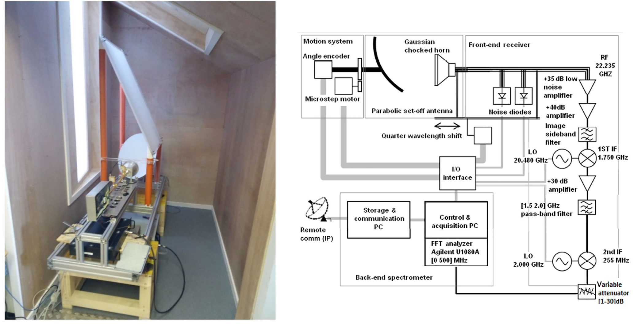
Figure 1A photo of VESPA-22 installed at the THAAO, Thule Air Base, Greenland (left), and the layout of the instrument (right).
A first uncooled low noise amplification stage amplifies the incoming signal with a gain of 35 dB. Two noise diodes manufactured by Noisecom are inserted in the radio frequency (RF) chain after the choke antenna by means of two 20 dB broadwall direction couplers. These two diodes produce a signal which is measured to average at about 119 and 78 K and are used to calibrate the sky signal observed by VESPA-22, as described in Sect. 3.3.
After the 20 dB couplers the signal is amplified and down-converted to lower frequencies and eventually sampled at 1 Gs s−1 by a fast Fourier transform spectrometer (FFTS; Acquiris AC240/Agilent U1080 A-001) with 16 384 channels, resulting in a spectral resolution of 31 kHz for a total bandwidth of 500 MHz.
During measurements, the antenna is moved back and forth to change its distance from the mirror by in order to avoid multiple internal reflections of the signal which would cause the formation of standing waves affecting the observed spectrum. One full spectrum is obtained by averaging together two 6 min spectra collected with the antenna positioned at these two different distances from the mirror. Once a day, two photodiodes are employed to check and reset the correct distance between the antenna and the mirror.
VESPA-22 is installed indoors to protect it from the strong winds and storms which can occur during most of the year. The indoor installation prevents the deposition on the quasi-optical system of snow in winter and dust in summer, as well as the condensation of water droplets, therefore improving the durability of the equipment. Additionally, the parabolic mirror and its driving motor are not exposed to strong winds, and VESPA-22 is therefore characterized by a pointing offset that is very stable with time. The instrument is located in a small wooden annex (Fig. 2) to the main observatory in order to minimize the presence of metal surfaces which could also yield standing waves in the observed spectrum.
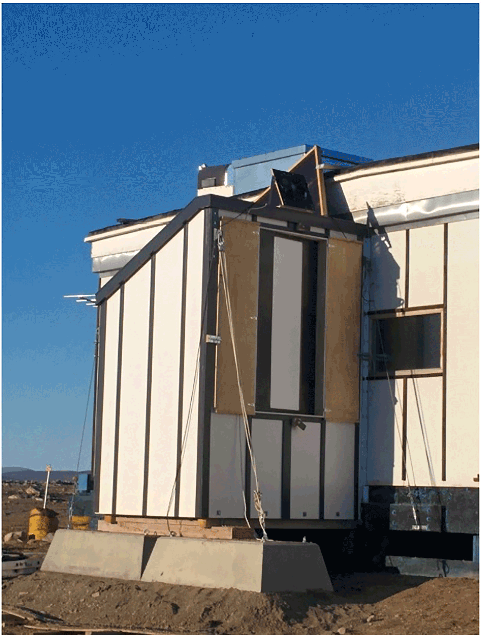
Figure 2A photo of the exterior of the wooden annex hosting VESPA-22. The observing window of the signal beam is visible on the side of the annex.
The spectrometer observes the sky through two 5 cm thick Plastazote LD15 windows, one covering the observation at angles from 10 to 60∘ above the horizon and a smaller one covering the zenith direction (see Figs. 1 and 2). This material was tested in the laboratory and proved to have a negligible absorption in the microwave region of interest. Furthermore, the windows are not perpendicular to the antenna beam in order to minimize any potential formation of standing waves. The opacity of the LD15 window sheets was estimated during VESPA-22 installation and it was measured to be less than 0.0005 Np. Three powerful fans are employed to blow off the snow from the observing windows, preventing deposition or ice formation on the external side of the windows. VESPA-22 compares the sky emission from the zenith direction (also called reference direction) to the sky emission from an angle close to the horizon (also called signal direction) in order to perform a stratospheric measurement, as will be explained in Sect. 3.2. The zenith is observed through a white Delrin® acetal homopolymer resin sheet, hereafter simply delrin (see Fig. 1), which adds a grey-body emission to the reference beam; this sheet is set at Brewster's angle with respect to the incident beam in order to minimize reflections and the formation of standing waves.
During an hour of standard instrument operations, about 3 min is dedicated to tipping curves (see Sect. 3.4) used to measure tropospheric opacity, about 35 min is dedicated to measure the emissions from the signal and reference beams, and the rest of the hour is dedicated to instrumental operations, such as the rotation of the parabolic mirror or the instrument calibration by means of the noise diodes.
VESPA-22 collects the 22.235 GHz radiation emitted by water vapor molecules. At this frequency, the Rayleigh–Jeans approximation for the Plank's law can be used and the radiation intensity can be expressed in terms of brightness temperature. The line shape of the emission from a stratospheric altitude z is mainly a function of atmospheric pressure:
where Δν is the line width, n<1 is a constant coefficient and T0=300 K (see Table 3, Sect. 4.1, for the spectroscopic values used for VESPA-22 retrievals). Using this dependence and knowing the pressure and temperature atmospheric profiles, the measured spectrum can be inverted using the reverse problem theory to obtain the vertical water vapor mixing ratio profile. In the mesosphere, the Doppler broadening overcomes the pressure broadening of Eq. (1) determining an upper limit to the altitude range in which the water vapor profile can be retrieved. In the lower stratosphere, the broadening makes the line width comparable to the VESPA-22 spectral bandpass, therefore setting a lower altitude limit for the deconvolved profile.
3.1 Atmospheric opacity
The majority of the incoming radiation measured by VESPA-22 comes from the troposphere. The tropospheric emission needs to be filtered in order to study the stratospheric signal. In order to simplify the radiative transfer equation, the following approximations can be adopted (e.g., Nedoluha et al., 1995).
-
The troposphere is represented as an isothermal layer absorbing the signal to be measured. The first kilometers of the atmosphere produce the greatest part of this layer emission which has a line width larger than VESPA-22 bandwidth. This contribution is treated as an emission constant in frequency.
-
The contribution of the stratospheric water vapor absorption to the opacity τ is small. This approximation was tested by calculating the atmospheric opacity by means of the radiative transfer simulation software ARTS (Eriksson et al., 2011) and using water vapor vertical profiles with and without their stratospheric component. At the frequency of maximum absorption, the contribution of the stratospheric profile to the overall atmospheric opacity is between 2 and 5 % depending on the season. When averaged over the VESPA-22 frequency range, the difference between the opacity calculated using a full water vapor vertical profile and a profile with no water vapor above the tropopause is between 0.4 and 1.5 %.
-
The opacity τν can be substituted by its mean value τ. The maximum difference between τν and its mean value τ is between 1.6 and 3.6 % depending on season.
-
The only signal coming from outside the atmosphere, T0, is the cosmic background radiation with a constant brightness temperature of 2.73 K.
With these approximations the radiative transfer equation describing the radiation received at the ground from an elevation angle θ can be written as
The left term is the radiation received by the spectrometer when pointing at the elevation angle θ. The first term on the right side is the extra-atmospheric emission, the second term is the solution of the radiative transfer equation for an isothermal domain where the tropospheric emission is indicated with Ttrop and represents the mean tropospheric temperature weighted with the water vapor concentration. The third term on the right is the emission coming from the stratosphere and mesosphere, T(ν), proportional to the air mass factor μ and attenuated in the troposphere by a factor e−μτ. The air mass factor at the elevation angle θ is computed according to the formula presented in the work of de Zafra (1995).
3.2 Beam-switching technique
The technique that VESPA-22 employs to measure the stratospheric signal is called the beam-switching technique or Dicke switching technique (e.g., Parrish et al., 1988). The instrument compares the emission coming from an observation angle θ (signal beam) with a reference signal with the same mean power over the passband. The observation angle depends on the atmospheric opacity and for VESPA-22 it varies from 12 to 25∘ above the horizon. The reference signal used by VESPA-22 is the sky emission at the zenith (reference beam). In clear-sky conditions, the emission at the zenith is smaller than the emission at a much larger zenith angle. Therefore, in order to ensure that the reference beam has the same mean power of the signal beam, a thin sheet of delrin is inserted in the reference beam. The delrin sheet acts as a grey body so that
where TR is the radiation observed by VESPA-22 coming from the zenith, partially absorbed by the delrin sheet, Td is the physical temperature of the sheet and τd its mean opacity value over the spectral passband. In this equation, the air mass factor μ is equal to 1.
During data-taking operations, VESPA-22 alternates reference and signal observations. The instrument constantly checks if the two beams have the same mean power and continuously changes the signal angle to minimize the difference between them. When the two beams have the same intensity, the frequency independent terms of Eqs. (3) and (2) can be equated, obtaining
where the stratospheric contribution to the mean beam intensity (about 1 %) is neglected (de Zafra, 1995).
The stratospheric signal T(ν) is obtained by subtracting reference from signal. Using Eqs. (2), (3) and (4) it is possible to write
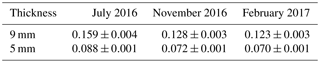
Three delrin sheets with different thicknesses (3, 5, and 9 mm) and opacities can be employed, depending on the season, in order to maintain the signal angle between 12 and 25∘ above the horizon. Spectra collected are smoothed using a 50-channel moving average. This smoothing process is, however, not performed in a 6 MHz interval centered around the emission line to maintain the maximum frequency resolution near the line peak.
In order to estimate τd, the mean opacity value of delrin over the spectral passband, during normal data-taking operations the signal angle is locked to its balanced position and the delrin sheet is removed from the reference beam. τd can then be calculated using
where is the mean intensity of the reference beam without the sheet and is the mean value of the signal beam. The brightness temperatures and are calculated using parameters obtained by means of a calibration performed using liquid nitrogen (LN2; see Sect. 3.3) which is always carried out before estimating τd. In order to run these operations, qualified personnel must be at the observatory and therefore τd was measured only in July and November 2016 and February 2017 (Table 1). A total of seven measurements of the compensating sheet opacity were performed, two in July, three in November, and two in February 2017. Half of the difference between the minimum and maximum τd values obtained during the same period is used as measurement uncertainty. The mean value of the delrin opacity changes with time, possibly due to a certain level of degassing, i.e., the property of absorbing/releasing water vapor molecules from/to the environment, which depends on atmospheric humidity and is often noticed in plastic materials. During winter, as the air is drier, the compensating sheets appear to release some water vapor and lower their opacities. VESPA-22 spectral data are calibrated using a linear interpolation between the τd values measured over time.
3.3 Calibration scheme
The broad-band response of VESPA-22 to the signal coming from the sky can be written as
In this equation, V is the incoming signal in count numbers of the FFT back-end spectrometer, T is the signal brightness temperature, α the gain of the instrument, Trec the receiver noise temperature and V0 the “zero” signal of the FFTS. All the quantities represented in Eq. (8) are frequency dependent. The “zero” signal, which amounts to approximately 0.5 % of the incoming signal to the FFTS, is measured approximately every 15 min and it is subtracted to each signal and reference 15 min integration spectra which are eventually saved on the control and acquisition PC (see Fig. 1). Using Eq. (8), Eq. (6) can be written as
VESPA-22 measures the gain parameter α by means of the noise diode. As mentioned before, VESPA-22 has two different noise diodes, one used to perform regular calibrations and the second inserted to ensure the stability over time of the first one, as described by Gomez et al. (2012). During regular measurements, the calibration noise diode is switched on and its emission is added to the reference signal. The noise diode is then switched off and VESPA-22 measures only the radiation coming from the zenith. The gain parameter can be obtained by subtracting these two measurements according to
where VR+nd and VR are the signals expressed in count numbers measured with the noise diode turned on and off, respectively, and Tnd is the noise diode emission temperature at the various frequencies, estimated during a calibration procedure. The calibration consists in measuring the emission from two sources at two different known emission temperatures. The first source is a black body at ambient temperature made with an Eccosorb CV-3 panel by Emerson and Cuming; the second source is mainly the sky at an angle of 60∘ above the horizon. Every 3 or 4 months, approximately, the sky emission can be replaced by a second CV-3 panel immersed in LN2. The use of LN2 likely grants more accurate results, as the physical temperature of the emitting body has a smaller uncertainty with respect to the estimated sky temperature at 60∘, but the LN2 calibration cannot be performed automatically by the instrument and has so far been carried in July and November 2016 and in February 2017.
Table 1Mean values and SDs (standard deviations) of the measured opacity for the two used delrin sheets during different seasons.
The general calibration equations are described in what follows, whereas the tipping curve procedure that allows the use of the sky as calibration source is explained in Sect. 3.4. Knowing the emission temperature of two sources α, Trec, and Tnd can be obtained by using the following equations:
Thot and Tcold and Vhot and Vcold are the emission temperatures and the recorded count numbers of the two sources, respectively. For the black body, the emission temperature is assumed to be equal to its physical temperature.
The noise diode produces a signal that is measured to be quite stable in frequency. In fact, single-channel Tnd values are always within 1.5 % of the spectral mean of the diode temperature brightness . The spectra originated from black-body measurements (especially those from the CV-3 immersed in LN2) can be affected by standing waves and in order to avoid to transfer them in the calibrated sky spectral measurements, Tnd is averaged over the central 11 000 channels of the FFTS, as suggested by Gomez et al. (2012). Therefore, it can be written
where Vcold + nd(νi) is the value of channel i with the noise diode turned on, while Vcold(νi) is the value of the same channel with the noise diode turned off.
3.4 Tipping curve procedure
In this section, the tipping curve calibration technique employed to calibrate the noise diodes using the sky signal is described. The tipping curve procedure is performed twice every hour as it is also used to measure the atmospheric opacity needed in Eq. (9). During a tipping curve, VESPA-22 collects the radiation coming from different elevation angles, approximately every 5∘ from 35 to 60∘ above the horizon. The measured spectra are averaged using the 11 000 central channels of the spectrometer. Radiation from the stratosphere contributes less than 1 % and can be neglected, so the signal intensity can be described by means of the following equation:
The atmospheric temperature Ttrop can be estimated from the surface temperature Tsurf:
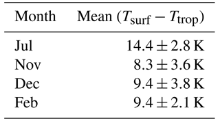
where the value of d can be affected by seasonal variations. In order to characterize this parameter several radiosoundings were launched during July, November, and December 2016 and February 2017. The value of the parameter d as a function of time is obtained from a linear interpolation between the mean values of Tsurf−Ttrop measured during these four periods, as described in Table 2. Ttrop is the average temperature obtained from radiosonde data by weighting the tropospheric temperature vertical profile with the water vapor concentration profile. Using Eq. (15), it is possible to explicitly give the relation between the opacity and the mean brightness temperature of the received signal:
A linear regression of the opacities observed at θi and the air mass factors μ(θi) allows us to retrieve the opacity at the zenith, τ (Nedoluha et al., 1995). Substituting for using Eq. (8) and approximating all the spectral quantities with their mean values (indicated by a bar) over the central 11 000 channels, Eq. (17) can be written as
where it appears that the mean values and are needed to perform the calculation.
Table 2Mean values and SDs of Tsurf−Ttrop obtained from the radiosoundings.
The emission from two calibration sources at different temperatures is used to calculate and according to Eqs. (11) and (12). However, since the sky emission temperature is not known, an iterative procedure is used to obtain both τ and . An initial opacity value, τ0, is adopted as a first guess to obtain using Eq. (21) with . is then used to obtain α0 and by means of Eqs. (11) and (12); μ(θi)τ is calculated for different elevation angles using Eq. (18), and ultimately a linear fit allows us to calculate a new estimate for τ, τ1. The iterative procedure goes on until the intercept value is minimized. Figure 3 shows the results of a tipping curve measurement carried out on 10 December 2016.
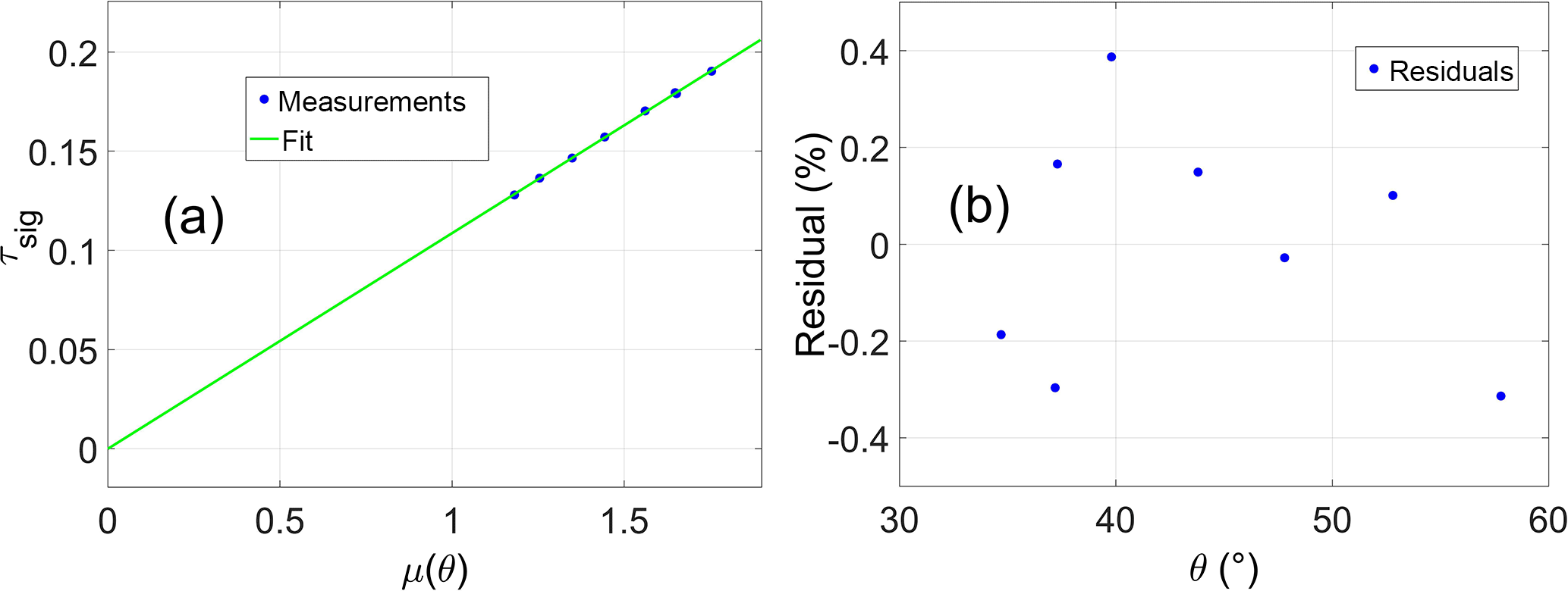
Figure 3(a) The values of (indicated with τsig on the y axis of panel a) as function of the air mass factor μ(θi) (blue points) measured during a tipping curve on 10 December 2016, and the fit result (green line). (b) The residuals (measurements minus fit) as a function of the elevation angle.
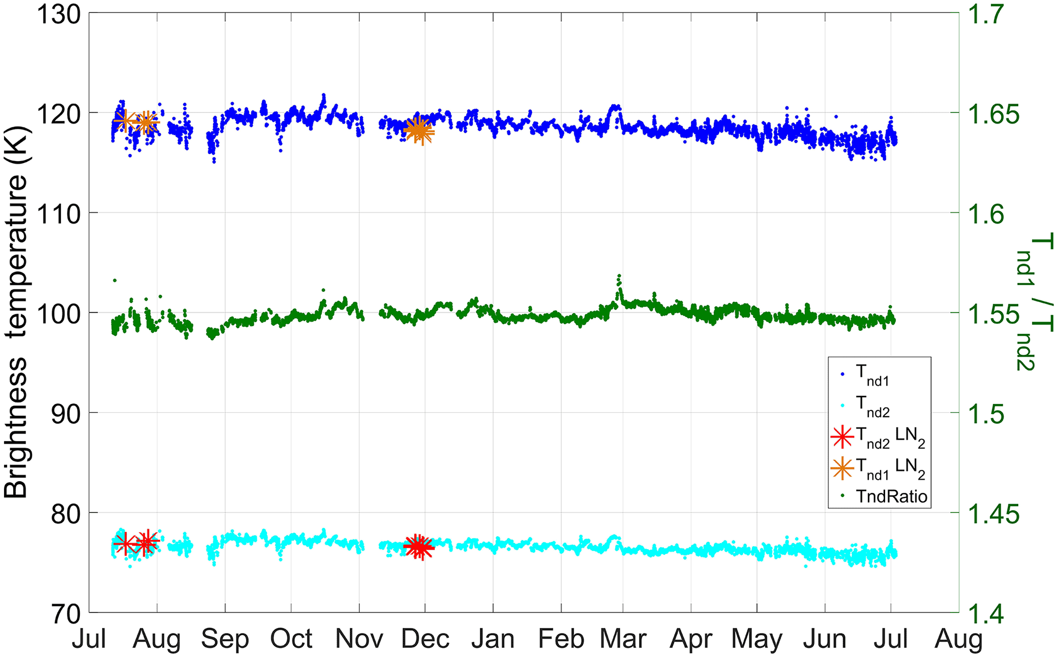
Figure 4Time series of the noise diodes mean emission temperature calculated by means of the tipping curve procedure (blue and cyan solid circles) compared with values obtained by means of LN2 calibrations (orange and red stars). The green dots and the right y axis display the ratio of the emissions from two noise diodes.
The value of measured with this procedure is used in Eqs. (11) and (13) to estimate . In order to avoid the use of data acquired during inhomogeneous sky conditions, all measurements producing linear fits (see Fig. 3a) with a root mean square larger than 0.4 are discarded. Figure 4 shows the time series of both noise diodes' mean emission temperatures (blue and cyan) and their ratio (green dots and right y axis) from July 2016 to July 2017. The noise diode in blue is the one used as calibration diode. In the same plot, values obtained using a LN2 cooled CV-3 as the cold load are also depicted (orange and red stars). The mean relative difference between values calculated with LN2 and with tipping curves carried out immediately before or after LN2 calibrations is (0.4±0.4) and (0.2±0.3) % for the calibration and the backup diodes, respectively. The ratio between the two noise diodes can provide insights into potential drifts of one diode with respect to the other. Since the estimated uncertainty on such a ratio is 0.05 (3.4 %), there appears to be no drift in the time frame discussed in this work.
VESPA-22 water vapor vertical profiles are obtained using the optimal estimation theory (Rodger, 2000). In what follows the retrieved water vapor profile is indicated as x, whereas xa indicates the a priori profile and the real water vapor atmospheric profile. The quantities y and ya represent the measured and a priori spectra, respectively. The matrix K is the weighting functions matrix, whereas Se and Sa are the covariance matrices associated to the spectral measurements and the a priori vertical profile, respectively. The profile x can be used to calculate the synthetic spectrum yfit according to
The altitude grid used for VESPA-22 retrievals starts from 10 km and goes up to 110 km altitude, at steps of 1 km. This range is much larger than the sensitivity interval of the instrument, which is in fact limited by the Doppler broadening at high altitudes and by the FFTS bandwidth and the tropospheric influence on the lower stratosphere at low altitudes. Only the central 400 MHz of the measured spectrum are used in the retrieval. The Sa matrix is computed according to
where σi is the root mean square of the variance of the a priori profile (expressed in volume mixing ratio, or vmr; see Fig. 5) at the altitude zi, while h is a correlation altitude set to be 5 km. Values of σi were empirically chosen in order to optimize the characteristics of the retrieval (i.e., maximize sensitivity range and vertical resolution without introducing unphysical oscillations in the retrieved vertical profile).

Figure 5The value of σi used to compute the a priori covariance matrix as a function of altitude (Eq. 20).
In the inversion process for VESPA-22 spectra, Se is a diagonal matrix with its diagonal elements all equal and calculated using a two-step process. A first retrieval of the original, not smoothed (see Sect. 3.2), spectral measurement averaged over 24 h is performed using a fixed value () for the Se diagonal elements and the obtained profile, x0, is used to calculate a synthetic spectrum y0,fit by means of Eq. (19). In order to consider the spectral measurement noise in the retrieval process, a second and final inversion is then performed, this time with the Se diagonal elements set to the mean value and the spectrum smoothed as indicated in Sect. 3.2. Note that also in this second inversion the diagonal elements of Se are held constant. For a 24 h integration time the Se diagonal values range from K2 (maximum value during summer) to K2 (minimum value obtained during winter).
A second-order polynomial (light blue curve in Fig. 7a) is also added to the retrieval in order to take into account the spectral emission from the upper troposphere and lower stratosphere, as well as a potential contribution to the baseline from the delrin sheet. The polynomial is calculated independently for each retrieved profile. The addition of this extra degree of freedom to the retrieval process reduces the altitude interval in which VESPA-22 retrievals can be considered reliable, raising the lower limit of the sensitivity range (see definition below and Fig. 8b) by approximately 6 km altitude. The use of a second-order term also introduces an additional source of uncertainty into the retrieved mixing ratio profile. Such a contribution is taken into account in the error analysis discussed in Sect. 4.3 (see Fig. 11).
An important quantity used to characterize the retrieval quality is the averaging kernels matrix A (Rodgers, 2000). The rows of A are called averaging kernels (AKs) and can be used to characterize the sensitivity of the water vapor retrieval at a given altitude to variations in the water vapor concentration profile at all altitudes (Rodger, 2000). If the AKs are well-peaked functions, centered at their nominal altitude, a perturbation in the atmospheric water vapor concentration at a specific altitude is transferred by the algorithm to the correct altitude layer of the retrieved profile. Furthermore, the area enclosed under each AK is an indication of the total sensitivity of the retrieved value at that altitude to atmospheric variations in water vapor concentration. A sensitivity value close to 1 at a certain altitude indicates that the major contribution to the retrieved value at that altitude comes from the spectral measurements rather than from the a priori water vapor profile. Following what was indicated by Tschanz et al. (2013), VESPA-22 retrievals are also considered valid for scientific use in the altitude range where the sensitivity is above 0.8. The AKs' FWHM can be used as a rough estimate of the local vertical resolution of the obtained water vapor mixing ratio vertical profile.
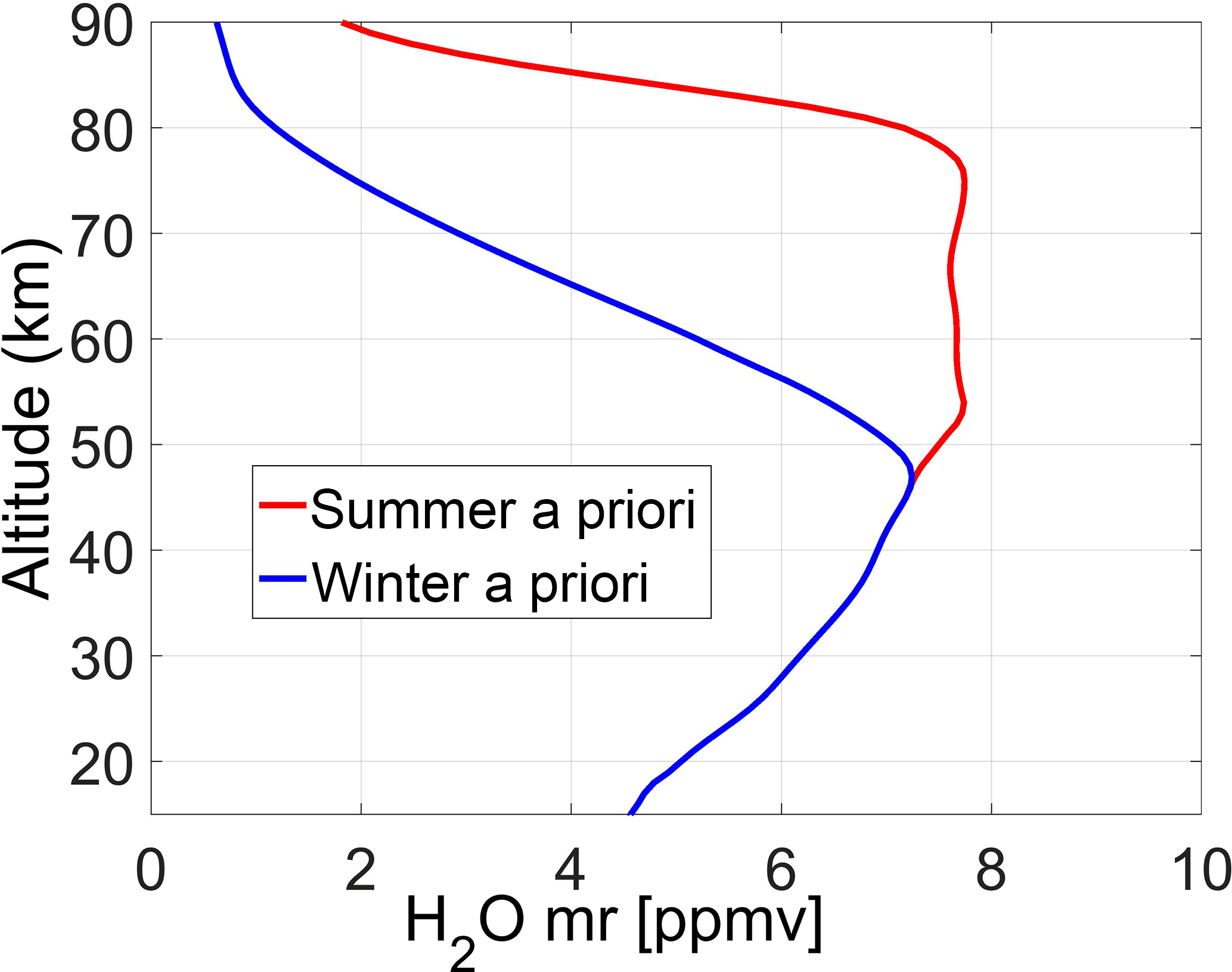
Figure 6The a priori profiles employed by VESPA-22 for the October–April period (indicated as winter a priori, blue line) and for the June–August period (indicated as summer a priori, red line) obtained from climatology.
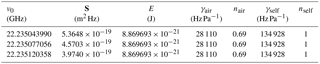
Table 3Spectroscopic parameters (“reference” model) used for VESPA-22 retrievals. Indicated parameters, from left to right, are emission line frequency, intensity, lower state energy, pressure broadening coefficient, pressure broadening temperature dependence, self-broadening coefficient, and self-broadening temperature dependence. The line intensity is given for a reference temperature of 296 K.
4.1 Forward model and a priori profiles
Figure 6 displays the a priori profiles used by the VESPA-22 retrieval algorithm during 10 out of the 12 months of the year and based on local climatology (3 years' worth of data of Aura/MLS v4.2). These profiles are identical below 48 km and diverge above, due to the large difference in polar regions between summer and winter water vapor mesospheric profiles. The summer a priori (red line) is used during the period from 1 June to 15 September, while the winter a priori (blue line) is used during the period from 16 October to 30 April. During the month of May and from 16 September to 15 October, there are transition periods in which a linear daily interpolation from one a priori to the other was used for continuity.
The matrix K and the ya spectrum are calculated using the radiative transfer simulation software ARTS (Eriksson et al., 2011), adopting a Voigt–Kuntz lineshape and the line intensity provided by the JPL 2012 catalogue (Pickett et al., 1998, and https://spec.jpl.nasa.gov/). Following the work of Seele (1999) and Tschanz et al. (2013), the line described by the JPL 2012 catalogue is divided into three emission lines indicating the hyperfine splitting of the 22.235 GHz water vapor line. The employed pressure broadening and self-broadening parameters are those reported by Liebe (1989). Table 3 summarizes the spectroscopic parameters used for the analysis of VESPA-22 spectral measurements which, in what follows, are indicated as the “reference” model.
The profile xARTS is the profile used in the forward model calculations to compute the a priori spectrum and the weighting functions. xARTS matches the a priori profile from 12 km of altitude upward and, below 9 km, it is consistent with the measurements of precipitable water vapor (PWV) collected by the HATPRO radiometer (Rose and Czekala, 2009; Pace et al., 2015) installed at the THAAO. This lower part of xARTS is calculated according to
where xEu is a water vapor mixing ratio profile obtained by daily smoothing monthly averages calculated from the radiosoundings launched from the Eureka station, PWVEu is the associated water vapor column content, and PWVHatpro is the column content measured by the HATPRO located at the THAAO. Data from Eureka were chosen (instead of those from Alert, Canada, for example) because they show the closest resemblance to the tropospheric profiles measured at Thule by local radiosoundings, when the latter are available. In order to avoid discontinuities in xARTS, values at altitudes between 9 and 12 km are obtained with a linear interpolation between xARTS(9 km) and xARTS(12 km).
The pressure and temperature profiles needed to run the forward calculation are built merging NASA Goddard Space Flight Center (GSFC), Aura/MLS and climatological temperature and pressure profiles. The NASA GSFC profiles obtained through the Goddard Automailer Service (Lait et al., 2005) are used to build the tropospheric meteorological state, from the ground up to 9 km of altitude. Between 10 and 87 km altitude, the MLS temperature and pressure profiles collected during VESPA-22 observations, in a radius of 300 km from the observation point of VESPA-22, are averaged together to produce a single set of daily meteorological vertical profiles. The VESPA-22 observation point coordinates are chosen to be 74.8∘ N and 73.5∘ W, and represent an estimate of the geographical coordinates of the air mass that is observed by VESPA-22 (which points southwest, at about 220∘) at 60 km altitude when the instrument aims at an elevation of 15∘ above the horizon. Daily temperature and pressure profiles from 97 to 110 km of altitude are obtained by daily smoothing zonal monthly averages from the COSPAR International Reference Atmosphere (Fleming et al., 1990).
The absence of vertical discontinuities in the temperature and pressure daily profiles is assured by a smoothing process performed at the altitudes where the three different datasets (GSFC, MLS, and COSPAR) are stitched together, between 9 and 12 km and between 87 and 97 km.
The software ARTS is employed to simulate the emission from the zenith, , and from an angle close to the horizon, ys. The emission is then rescaled using Eq. (22), therefore simulating the effect of the delrin compensating sheet:
whereas the mean difference ys−yr is
The opacity τd used in Eq. (22) is the opacity of the compensating sheet; the temperature Td is the temperature of the sheet, measured by a sensor installed next to it; and the signal beam observing angle, , is chosen in order to minimize the mean difference ys−yr, as it is in fact attained by VESPA-22 in its data-taking process. The a priori spectrum is calculated according to the same equation used for the measured signal (Eqs. 5 and 6),
where and are the air mass factor associated to the simulated signal beam and the zenith opacity calculated from the xARTS profile.
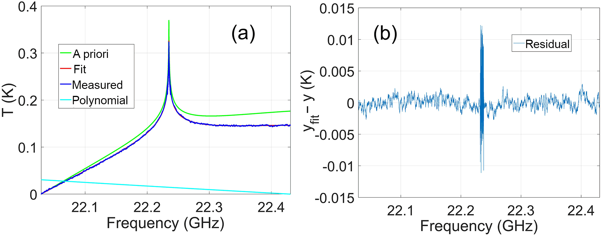
Figure 7(a) An example of VESPA-22 measured spectrum (blue) collected on 23 December 2016, with the a priori spectrum in green and the fit spectrum in red. The second-order polynomial is indicated with a cyan solid line. (b) The residual yfit−y. The central part of the spectrum is unsmoothed in order to maintain the maximum spectral resolution near the peak and its residual is larger.
Deriving Eqs. (24) and (22), and using the K matrix definition (Rodgers, 2000), the retrieval weighting function matrix can be written as
where Ks and Kr are the weighting function matrices that ARTS calculates for the simulated signal and reference beams. As a first approximation, the dependence of on the stratospheric water vapor profile in Eq. (25) is neglected.
4.2 Retrieval example
Figure 7a shows a VESPA-22 spectrum integrated for 24 h (blue line) on 23 December 2016, its corresponding synthetic spectrum yfit (red line) and the a priori spectrum (green line), while the residual (defined as the difference between fit and measured spectrum, yfit−y) is plotted in Fig. 7b. The cyan line is the second-degree polynomial retrieved by the inversion algorithm. Figure 8a shows the result of the inversion of the measured spectrum depicted in Fig. 7 with the a priori profile and retrieval 1σ uncertainty. The details on the uncertainty calculation are discussed in Sect. 4.3.
4.3 Retrieval uncertainty
The uncertainty characterizing VESPA-22 retrieved profiles can be divided into four major contributions: (1) the uncertainty due to the linear approximation used in the optimal estimation, (2) the uncertainty due to the various parameters used in the spectra calibration and pre-processing, (3) the uncertainty due to spectral noise and potential artifacts, and (4) the uncertainty introduced by the use of the second-order polynomial in the retrieval process. One additional error source is the limited vertical resolution inherent to concentration vertical profiles obtained by means of this ground-based observing technique. This leads to solution profiles that can be considered a smoothed version of the real atmospheric concentration profiles. In discussing the optimal estimation method, Rodgers (2000) suggests that this error, called “smoothing error”, should be estimated only if accurate knowledge of the variability of the atmospheric fine structure is available. This approach is used here and the smoothing error is not included in the error estimate.
The first contribution can be evaluated observing the difference Δylin between the fit spectrum without the addition of the second-order polynomial, , and the spectrum obtained using ARTS to calculate the emission expected from the retrieved profile x (in the calculation, ARTS does not perform any linear approximation):
The uncertainty Δxlin that Δylin causes on the retrieved profile can be calculated with
where G is the gain matrix (Rodgers, 2000). The uncertainty Δxlin has a negligible contribution to the total uncertainty (with a maximum of 0.1 % at 70 km altitude).
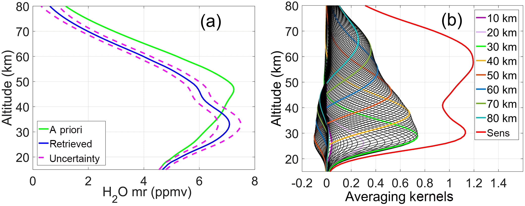
Figure 8(a) The retrieved VESPA-22 profile (blue solid line) correspondent to the spectrum showed in Fig. 7. The a priori profile is indicated with a green solid line. The two red dashed lines describe the uncertainty of this VESPA-22 retrieval (for details on the estimated uncertainty of VESPA-22 mixing ratio vertical profiles see Sect. 4.3). (b) Rows of the A matrix multiplied by a factor of 10 as a function of altitude (some A functions are highlighted in colors). The vertical profile of the sensitivity is shown in red.
Table 4Uncertainties on the various parameters used in the calibration process. When the uncertainty is a function of altitude the minimum and maximum values of the uncertainty are reported.
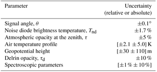
Figure 8b shows the corresponding averaging kernels (AKs, black and colored solid lines). AKs are multiplied by a factor of 10 and the sensitivity in indicated with a red solid line.
In order to evaluate the second contribution listed above, the effects on the retrieved profile due to the variation of each single parameter used in the measurements calibration and pre-processing was investigated. The difference between the profile retrieved using the “correct” value of a specific parameter and the retrieval obtained by changing such a value by the estimated relative uncertainty of the parameter is considered to be the contribution σi of this parameter to the total calibration and pre-processing uncertainty. The total uncertainty from these sources is defined as calibration uncertainty. Table 4 summarizes the uncertainties on the various parameters involved in the calibration and pre-processing of VESPA-22 spectra. When the uncertainty is a function of altitude the minimum and maximum values of the uncertainty are reported. The total calibration uncertainty σcal is given by
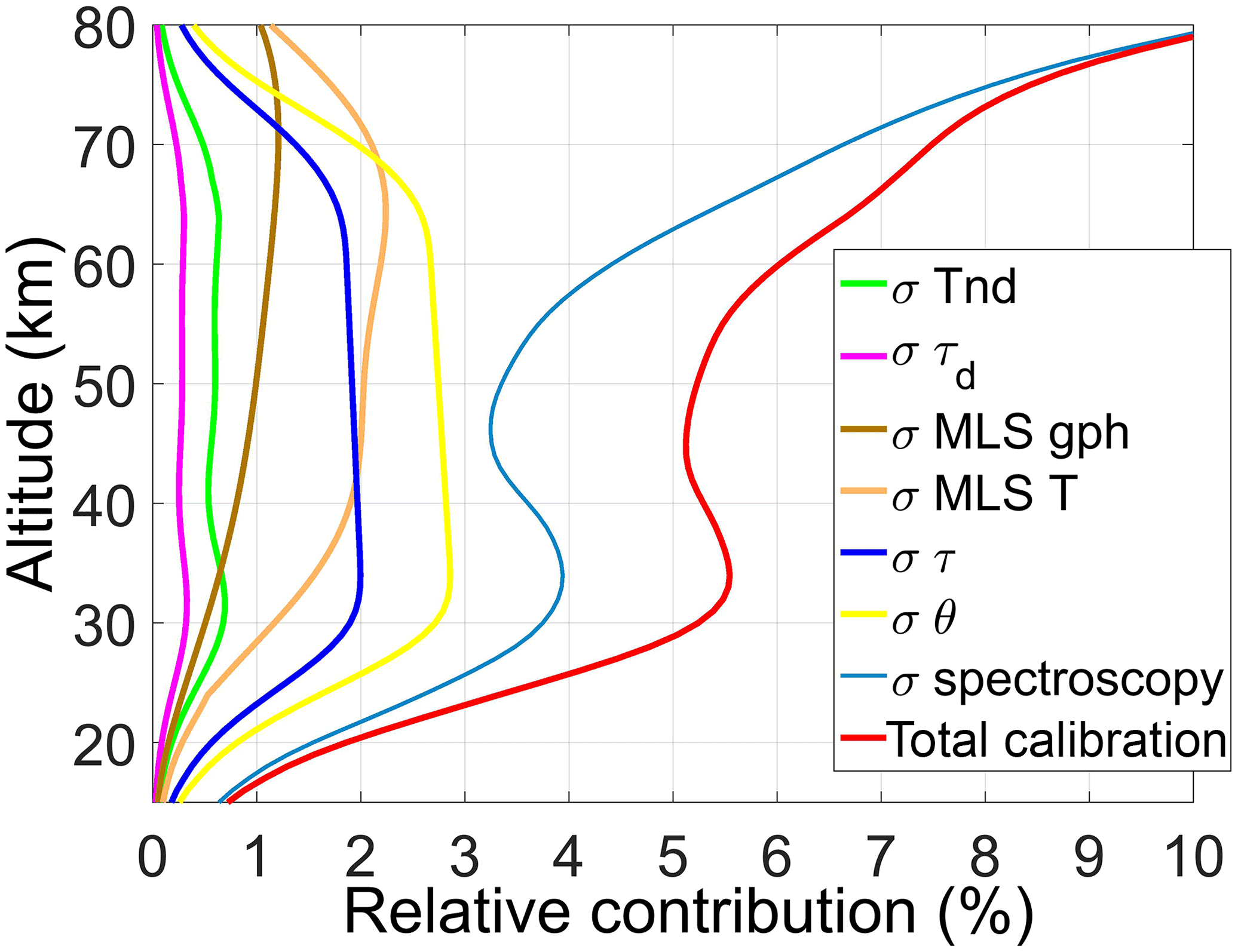
Figure 9Relative contributions to the calibration uncertainty defined by Eq. (28) and indicated with a red solid curve. The contributions are the signal beam angle (yellow), the noise diode temperature (green), the sky opacity (blue), the MLS meteorological profiles (orange and brown), the compensating sheet opacity (magenta), and the spectroscopic parameters (cyan).
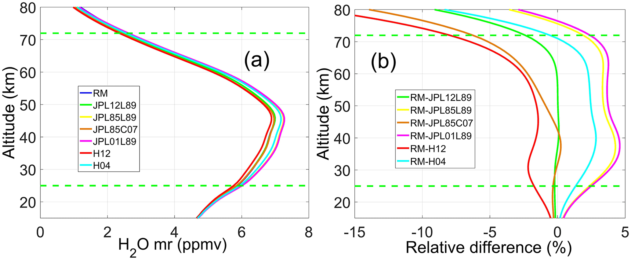
Figure 10(a) Mean retrieved water vapor profiles obtained using different spectroscopic models (the blue line is the model eventually adopted for the analysis of VESPA-22 spectra, called reference model, or RM). The spectroscopic parameters for the additional models tested are obtained from different versions of the JPL catalogue (years 1985, 2001 and 2012; Pickett et al., 1998) with the pressure broadening parameters taken from Liebe (1989) and Cazzoli et al. (2007). Two models include values from HITRAN 2004 and 2012 (Rothman et al., 2013). Models are indicated in the legend with their abbreviations: JPL2012Liebe1989 (JPL12L89), JPL1985Liebe, 1989 (JPL85L89), JPL1985Cazzoli, 2007 (JPL85C07), JPL2001Liebe, 1989 (JPL01L89), HITRAN2012 (H12), and HITRAN2004 (H04). (b) Vertical profiles of mean relative differences between VESPA-22 profiles obtained using the reference model and the different spectroscopic models. Data represented here range from 4 October 2016 to 22 May 2017. The average retrieval sensitivity range is marked by dashed horizontal green lines.
In Fig. 9, the relative contributions of the various parameters needed in the calibration and pre-processing procedures are shown. The yellow line shows the σi contribution due to the uncertainty on the signal beam angle. In order to minimize this contribution, the choked antenna and the parabolic mirror are aligned using a He-Ne laser. During the period from April to October, the VESPA-22 pointing offset can be verified by scanning rapidly at around the sun elevation angle and comparing the measured position of the center of the sun against the known ephemerides. For the measurements discussed here an offset of was estimated. The green solid line shows the potential relative error on the water vapor mixing ratio vertical profile due to the uncertainty on the estimated noise diode temperature . In order to evaluate the uncertainty on , the 0.4 % difference between the values obtained by means of the LN2 calibrations and by means of the skydips immediately following or preceding the LN2 calibrations (see Sect. 3.4 and Fig. 4) is considered. On top of this, the fluctuations of the signal produced by the calibration diodes must also be taken into account. These can be evaluated by using the standard deviation (SD) of the difference over time between the values of the two noise diodes, measured to be 1.1 %. The tipping curve procedure allows for calculation of the noise diodes brightness temperature averaged over the 11 000 central channels of the spectrometer. Since the noise diodes brightness temperatures do have a small frequency dependence, using their mean values introduces a source of uncertainty which is estimated to be 0.9 %. An additional source of uncertainty is due to sky inhomogeneities, and amounts approximately to 1 %. All these sources of uncertainty for are added in quadrature to obtain a total uncertainty of 1.8 %. The blue line shows the contribution due to the uncertainty Δτ on the sky zenith opacity τ. In order to estimate this uncertainty, the uncertainties introduced by sky inhomogeneity and by the estimation of the effective tropospheric temperature Ttrop are considered. The first contributes to about 2 % and is estimated using the uncertainty on the slope of the linear fit of the tipping curve (see Sect. 3.4 and Fig. 3). The second contribution can be evaluated observing the daily fluctuations of Ttrop measured at Eureka (Canada), Aasiaat (southern Greenland), and Alert (Canada). The natural day-to-day temperature fluctuations and the lack of tropospheric meteorological data at Thule during long intervals of time led us to estimate an uncertainty on Ttrop of about 6 K, which then makes the total uncertainty Δτ∼5 %.
The brown and orange lines show the σi's due to temperature and geopotential height profiles used in the forward calculation. The uncertainties on these parameters are obtained from the MLS data quality and description document (Livesey et al., 2015). In Fig. 9, the magenta line shows the contribution of the uncertainty on the compensating sheet opacity, Δτd. Although the uncertainty on the measurements of τd is about 2 % (see Table 1), the use of a linear interpolation suggests the use of a more conservative estimate, eventually set at 10 %. The cyan line shows the contribution due to uncertainties in the employed spectroscopic parameters, and it has the largest impact on the calibration uncertainty. Following Straub et al. (2010), the emission line intensity and the pressure broadening coefficient were assigned an uncertainty of m2 Hz and 1014 Hz Pa−1, respectively.
In addition to these uncertainties, Fig. 10 shows the results of retrieving VESPA-22 data from October 2016 to May 2017 using different sets of values for the spectroscopic parameters (see also Haefele et al., 2009). In the figure, the mean profiles retrieved using the different models listed in the legend are depicted. Such models include values taken from HITRAN (Rothman et al., 2013) and JPL catalogues (Pickett et al., 1998), for different years, and from Liebe (1989) and Cazzoli et al. (2007). The blue line represents the mean profile obtained using VESPA-22 reference model (RM). In Fig. 10b, the mean relative difference profiles between retrievals obtained using the reference model and the other spectroscopic models are drawn (see legend). The water vapor mixing ratio retrieved profiles show a strong dependence on the spectroscopic model of choice, with a relative difference between profiles obtained using different models reaching a maximum of 8 % at the top of the sensitivity range.
Figure 11 shows the uncertainty calculated for the retrieval of 23 December 2016, shown in Fig. 8. The overall calibration uncertainty is shown with a red curve. The uncertainty due to spectral noise and artifacts can be evaluated using the S uncertainty matrix (Rodger, 2000) obtained as
The square root of the diagonal elements of S represents the spectral uncertainty of the retrieved profile at different altitudes and is indicated in Fig. 11 with a blue line. This term depends on the Se value of the retrieval and its value increases during summer and with poor weather conditions. As mentioned in Sect. 4, the diagonal values of the Se matrix are held constant and do not take into account the spectral noise reduction obtained with the 50-channel smoothing process which is applied to most of the spectrum (Sect. 3.2). This may lead to a small overestimation of the spectral uncertainty depicted in Fig. 11 in the altitude range 20–50 km (with a maximum potential overestimation of 0.3 % at 25 km altitude). The green curve displays the estimated uncertainty due to the use of the second-order polynomial in the retrieval process. The total uncertainty is calculated as
and is represented with a purple line in Fig. 11.
VESPA-22 water vapor vertical retrievals obtained from 24 h integration spectra (from 00:00 to 23:59 UT) have been compared with version 4.2 of Aura/MLS water vapor vertical profiles. The MLS profiles used for this intercomparison are daily mean profiles obtained averaging all MLS profiles collected within a radius of 300 km centered around VESPA-22 observation point (74.8∘ N, 73.5∘ W; see Sect. 4.1).

Figure 11Vertical profiles of the calibration uncertainty (red), the retrieval uncertainty (blue), and the total uncertainty (magenta) of VESPA-22 water vapor mixing ratio vertical profiles obtained inverting a spectrum collected on 23 December 2016 and integrated for 24 h.
The intercomparison is carried out using data from 15 July 2016 to 2 July 2017. In general, spectra collected during July, August, and September are less continuous and noisier than spectra observed during the rest of the selected period. This is due to extensive testing of the equipment, poor weather conditions, and snow covering the zenith observing window (in November 2016 a second powerful fan was installed outside the roof window in order to reduce snow deposition). Furthermore, there are no stratospheric measurements carried out by VESPA-22 between 4 and 22 November 2016, due to snow covering the lower portion of the reference beam window. A few isolated days in which large sky inhomogeneities do not allow the correct balance of signal and reference beams have also been removed from the intercomparison. It is worth recalling that the signal-to-noise ratio of VESPA-22 spectra, and therefore the quality of the retrievals, depends on the sky opacity and, consequently, on the season, being noticeably better during winter and poorer in summer. This is particularly true for microwave spectrometers operating in polar regions, where seasonal fluctuations of the tropospheric water vapor column content are significant.
Table 5 summarizes the characteristics of the Aura/MLS water vapor version 4.2 retrievals (Livesey et al., 2015). In order to compare the two datasets, MLS vertical profiles are convolved with VESPA-22 averaging kernels in order to match the resolution of VESPA-22 profiles according to Rodgers (2000):
where is the raw (high resolution or HR) MLS water vapor vertical profile, xa is the a priori profile, A is the averaging kernel matrix, and xMLS is the convolved MLS profile. Additionally, VESPA-22 profiles were also compared with MLS profiles smoothed in the vertical by using a 10 km moving average. This second set of degraded MLS profiles was generated in order to study the correlation between VESPA-22 and MLS datasets without introducing the dependency from one another brought by the convolution process (affecting MLS convolved profiles).
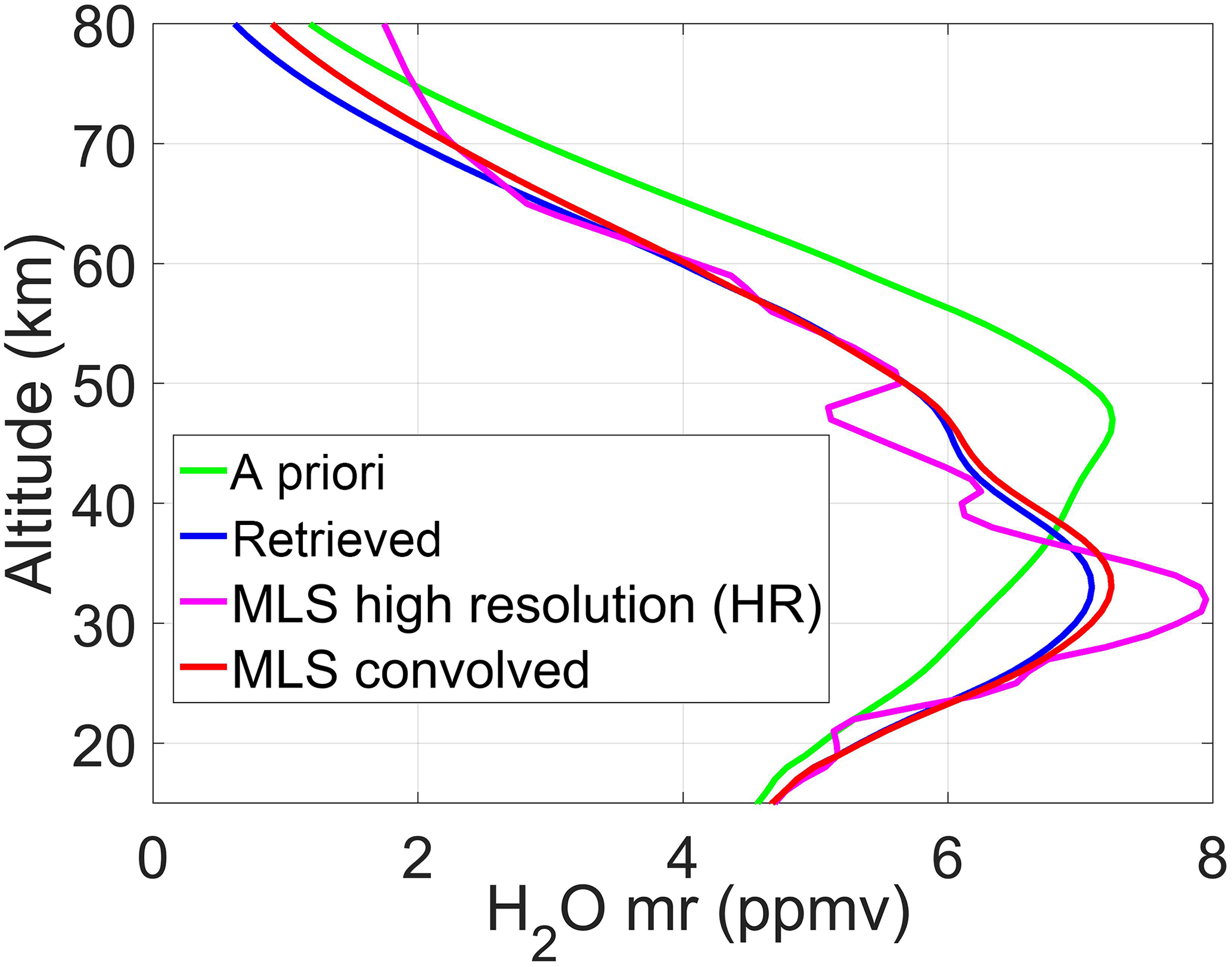
Figure 12The MLS profile measured on 23 December 2016, with its high original vertical resolution (HR, magenta line) compared with the a priori profile (green line), the MLS convolved profile obtained from Eq. (31) (red line), and the VESPA-22 retrieved profile (blue line).
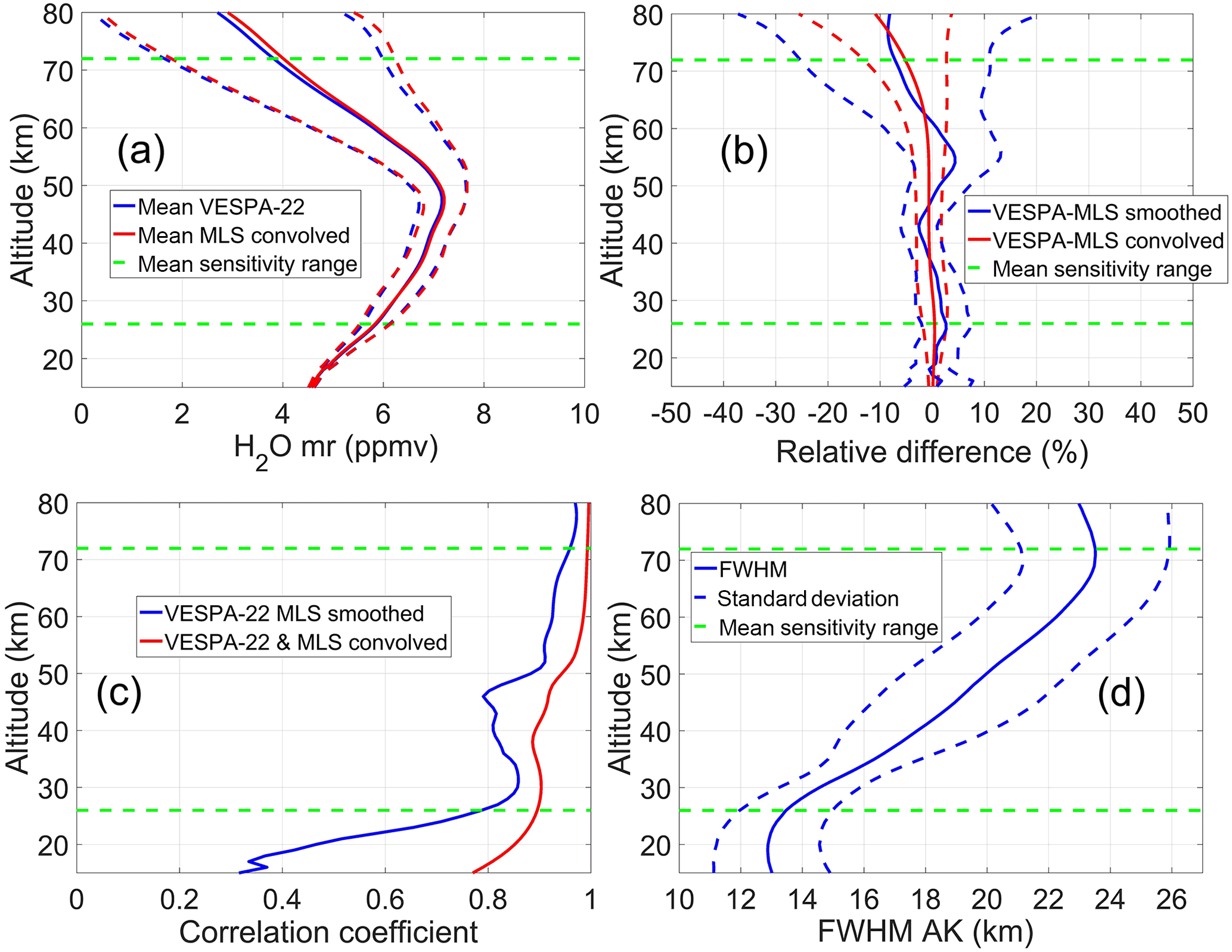
Figure 13(a) VESPA-22 averaged water vapor mixing ratio vertical profile with its SD (blue line and blue dashed lines) and the mean MLS convolved profile with its SD (red line and red dashed lines); (b) vertical profiles of the mean relative difference between VESPA-22 and MLS convolved (red line), and between VESPA-22 and MLS smoothed (blue line) with their SDs (red and blue dashed lines, respectively); (c) vertical profiles of the correlation coefficient between VESPA-22 and MLS convolved profiles (red line), and between VESPA-22 and MLS smoothed profiles (blue line); (d) vertical profile of the mean FWHM of VESPA-22 averaging kernels with its SD. The data used for the intercomparison range from 12 July 2016 to 2 July 2017. The green dashed horizontal lines display the mean altitudes of the sensitivity range extremes.
Table 5The main specifications of Aura/MLS water vapor mixing ratio profiles version 4.2 (Livesey et al., 2015).
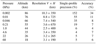
Figure 12 shows the MLS measured profile on 23 December 2016 (magenta line), the MLS convolved profile obtained from Eq. (31) (red line), the a priori profile (green line), and the VESPA-22 retrieved profile (blue line) for the same day. The MLS convolved profile tends to the a priori profile below 26 km and above 72 km, where the retrieval sensitivity drops.
Figure 13a shows the mean VESPA-22 retrieved profile (in blue) and the mean MLS convolved profile (in red), with their SDs indicated with dashed lines. The mean sensitivity of VESPA-22 retrieved profiles is larger than 0.8 from about 26 to 72 km altitude and is indicated by the two green horizontal dashed lines. This interval can vary from day to day depending on the noise level of the 24 h integrated spectra (see white solid lines in Fig. 15). Figure 13b displays the relative difference of VESPA-22 water vapor mixing ratio mean vertical profile with respect to the MLS mean convolved profile (red line) and with respect to the MLS smoothed mean vertical profile (blue line) with their SDs (blue and red dashed lines, respectively). The largest relative and absolute (not shown) differences between the two datasets occur at 72 km, the upper limit of the VESPA-22 sensitivity range, and it is about −6 %, with Aura/MLS convolved mean profile being larger than VESPA-22 mean retrieval. The SD of the differences increases in the mesosphere as a result of the larger atmospheric variability and the larger relative uncertainty of both instruments at these altitudes (see Fig. 11 and Table 5) with respect to lower levels.
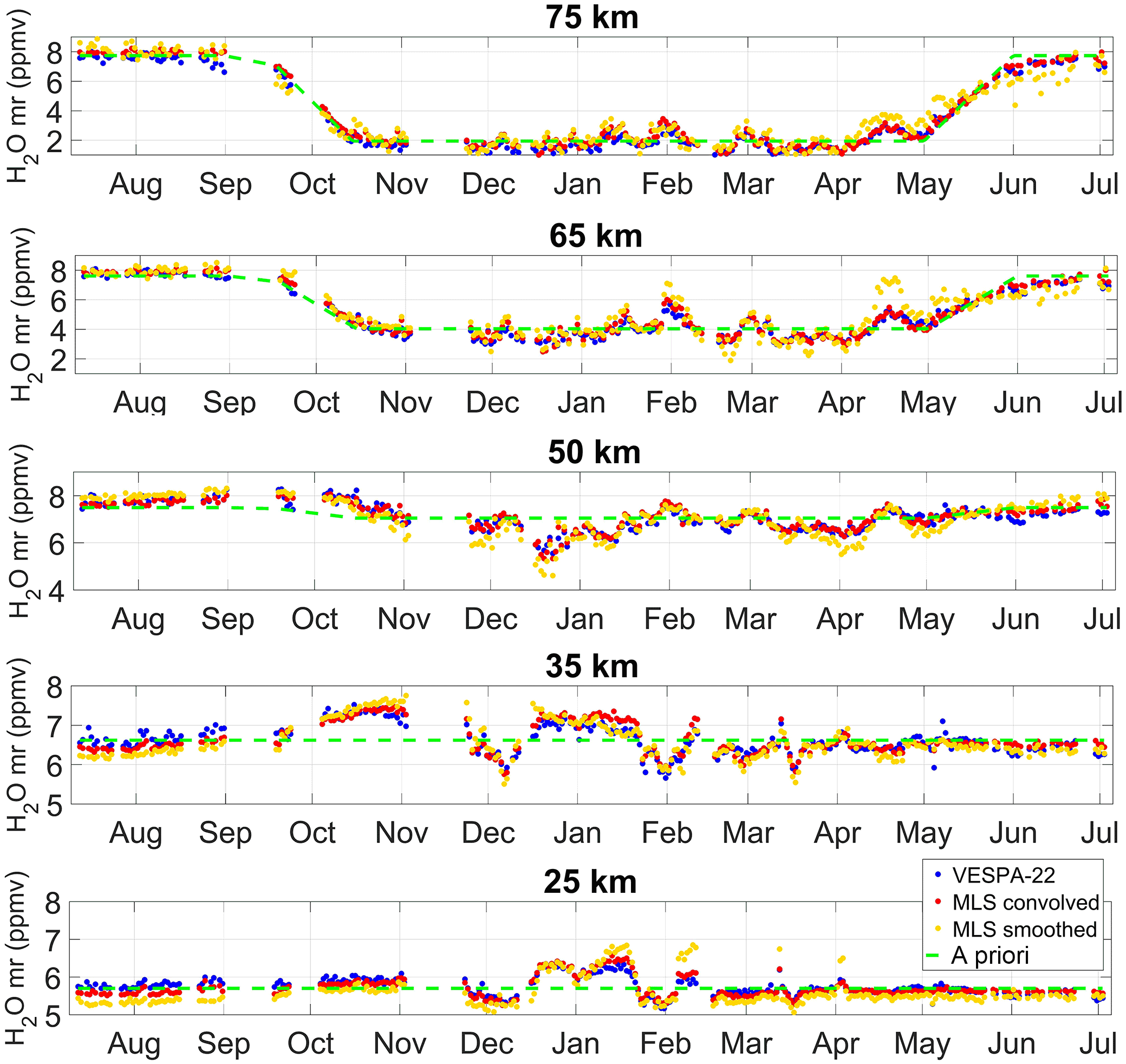
Figure 14Time series at different altitudes of water vapor mixing ratio values obtained with VESPA-22 (blue), by convolving MLS HR vertical profiles with VESPA-22 averaging kernels (red), and by smoothing MLS HR vertical profiles with a 10 km running average (yellow). Please note that the time series at the five different altitude levels have different scales on the y axis in order to better show the differences between datasets.
Figure 13c shows the vertical profiles of the correlation coefficient between VESPA-22 and MLS convolved data (red), and between VESPA-22 and MLS smoothed data (blue). The latter shows values of 0.8 or higher over the entire sensitivity range. The good correlation of VESPA-22 with MLS smoothed profiles down to 26 km altitude suggests that VESPA-22 retrievals are reliable at these stratospheric altitudes. Such a high correlation was obtained by using for the VESPA-22 retrieval algorithm an a priori profile held constant in time up to 48 km, therefore providing no contribution to the correlation. Below 25 km the correlation with MLS smoothed quickly deteriorates, whereas the correlation of VESPA-22 with MLS convolved profiles remains high, emphasizing the dependency of both datasets on VESPA-22 a priori profile and averaging kernels. Figure 13d shows the vertical profile of the mean values of the FWHM of VESPA-22 averaging kernels (blue solid line) calculated over the comparison period. The FWHM of the averaging kernels is a measure of the retrieval vertical resolution (Rodgers, 2000). The single-profile vertical resolution can vary depending on the level of noise affecting the measured spectrum.
Figure 14 shows the time series at different altitudes of water vapor mixing ratio values from VESPA-22 (blue dots), MLS convolved (red dots), and MLS smoothed (yellow dots) datasets. The 25 and 35 km water vapor time series display rapid and intense variations in winter caused by the polar vortex moving over Thule in mid-December and then away from Thule at the end of January. The 25 km time series is also useful to evaluate the quality of the VESPA-22 measurements at the bottom limit of the sensitivity range. Figure 14 shows that, at this altitude, VESPA-22 is capable of depicting the rapid variations in water vapor but does not have the necessary sensitivity to match the most intense variations observed by MLS (mid-January and early February). Both MLS and VESPA-22 time series at 65 km show a peak in mid-April, although VESPA-22 underestimates the peak intensity with respect to MLS possibly due to the reduced sensitivity of VESPA-22 retrievals at this altitude during spring.
In order to provide a more complete, albeit less quantitative, overview of the VESPA-22 and convolved MLS time series, Fig. 15 shows contour maps of VESPA-22 (in color) and MLS convolved (black lines) water vapor profiles. The data collected by both instruments reveal an absolute maximum in August 2016 at 50 km of height of about 8.3 ppmv. During fall and winter the maximum of the water vapor mixing ratio profile lowers its altitude to reach about 35 km in January 2017, due also to the downward motion of air inside the polar vortex. The two steep gradients in water vapor mixing ratio due to the polar vortex moving away from Thule are clearly visible between 25 and 40 km altitude.
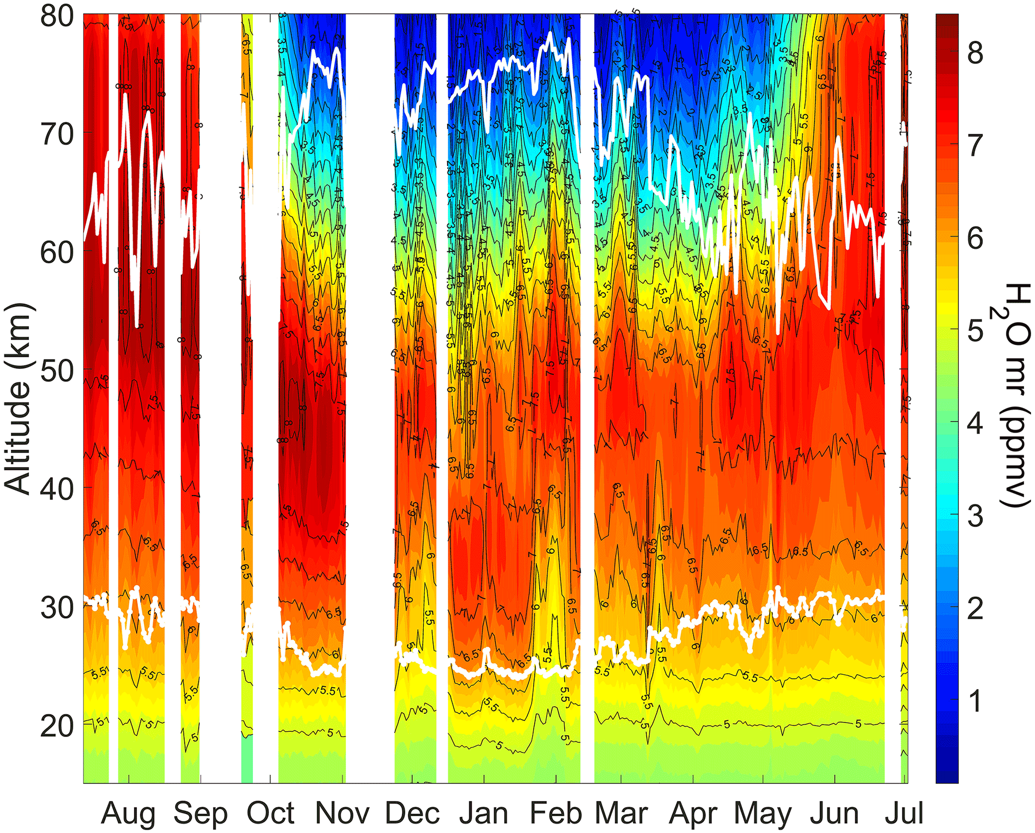
Figure 15A map showing the VESPA-22 retrieved profiles (colored areas) compared to MLS convolved profiles (black lines). The blank areas indicate the lack of VESPA-22 data for more than 3 days. White solid lines indicate the time series of the sensitivity interval.
Both instruments also observe the return of the water vapor mixing ratio to pre-winter values in mid-April, possibly indicating the occurrence of the vortex final warming, with the re-establishment of a maximum in the mixing ratio profile at about 50 km altitude.
VESPA-22 was installed at the Thule High Arctic Atmospheric Observatory (THAAO; http://www.thuleatmos-it.it/) located at Thule Air Base, Greenland, in July 2016 for long-term observations of the polar middle atmospheric water vapor and column content. The instrument is characterized by a FWHM encompassing 3.5∘ (Bertagnolio et al., 2012), granting the observation of the signal beam at angles as low as about 12∘ above the horizon. The instrument is installed indoor in a wooden annex to the main laboratory and observes the sky emission through windows made of 5 cm thick Plastazote LD15 sheets. During clear-sky conditions, there are no evident artifacts larger than 2 mK affecting the measured spectra. VESPA-22 operated automatically with minimum need for maintenance for about 1 year, proving the robustness of hardware and acquiring system.
The instrument calibration is regularly performed using two noise diodes. The emission temperature of these elements is measured during tipping curve calibrations and checked periodically with liquid nitrogen calibrations. The calibrating noise diode temperature is estimated with an uncertainty of 1.8 %.
VESPA-22 retrieval algorithm is based on the optimal estimation technique (Rodgers, 2000); the retrieved profiles from 24 h integration spectra have an average sensitivity larger than 0.8 from about 26 to 72 km of altitude and a vertical resolution from about 12 to 23 km. The forward model is provided by the ARTS software (Eriksson et al., 2011), which is tuned to reproduce the VESPA-22 measurement technique. In order to perform a realistic simulation of the troposphere, the PWV measured by the HATPRO radiometer (Rose and Czekala, 2009; Pace et al., 2015) operating side by side with VESPA-22 is taken into account in the forward model.
The uncertainty on VESPA-22 retrieved water vapor mixing ratio vertical profiles is evaluated as the sum of the contributions from calibration, pre-processing, spectroscopic parameters, measurement noise, and use of a second-order polynomial baseline in the retrieval process. In the sensitivity range of VESPA-22 retrievals, the total uncertainty is estimated to be about 5–6 % from 26 to 60 km, increasing to about 18 % at 72 km.
VESPA-22 and MLS water vapor profiles are compared during a period from July 2016 to July 2017. The VESPA-22 data used in the comparison are the results of retrievals from 24 h integration spectra, while MLS data are the daily mean vertical profiles collected by MLS in a radius of 300 km around VESPA-22 observation point, convolved with VESPA-22 averaging kernels. No significant biases were observed between the two datasets in the altitude range from 25 to 60 km, whereas from 60 to 72 km the value of the mean difference (VESPA-22 – MLS) increases, reaching −6 % (−0.2 ppmv) at 72 km. A good correlation is also found between VESPA-22 and MLS smoothed (see Sect. 5) vertical profiles in the entire vertical range (from 26 to 72 km altitude, on average) where VESPA-22 profiles are considered valid.
The results described in this paper proved that VESPA-22 is capable of carrying out reliable middle atmospheric water vapor measurements during different seasons and weather conditions, although the vertical range where the dataset is recommended for scientific use is reduced in summer with respect to winter. VESPA-22 retrievals are capable of correctly representing the rapid variations in water vapor concentrations that can occur in the stratosphere, as revealed by the large water vapor gradients measured both by VESPA-22 and Aura/MLS in mid-December 2016, late January/early February 2017, and then again during April and May (see Fig. 15). At the same time, VESPA-22 spectral measurements and corresponding mixing ratio retrievals appear to have the necessary stability and consistency to observe slow seasonal variations, such as the water vapor subsidence occurring inside and at the edge of the polar vortex.
The NDACC network maintains a database where all data are stored and are publicly available. Therefore, the dataset presented here will be publicly available, once the instrument is accepted in the NDACC network.
Until then, data can be accessed by contacting Giovanni Muscari (giovanni.muscari@ingv.it).
The authors declare that they have no conflict of interest.
This article is part of the special issue “Twenty-five years of operations of the Network for the Detection of Atmospheric Composition Change (NDACC) (AMT/ACP/ESSD inter-journal SI)”. It is not associated with a conference.
The development of VESPA-22 and measurements at Thule were supported by the
Italian Antarctic Programme (PNRA) funded by MIUR through projects 2013/C3.03
and 2015/B3.01. This study was also partially supported by Progetto Premiale
ARCA. Bob de Zafra, Mike Gomez, and Axel Murk helped with the development of
VESPA-22 by suggesting useful solutions to technical problems related to the
instrument design. We are indebted to them. Additionally, Giovanni Muscari is
very thankful to Nik Kämpfer and Axel Murk for donating to the VESPA-22
project the firmware that the FFTS is currently employing. We are grateful to
Stephan Buehler and Patrick Eriksson for helping with the ARTS software, and
to the MLS team of the Jet Propulsion Laboratory for providing access to the
Aura/MLS data. We thank Gerald Nedoluha and Axel Murk for their knowledgeable
and valuable comments to the manuscript initially submitted.
Edited by: Hal Maring
Reviewed by: Gerald Nedoluha and one anonymous referee
Bertagnolio, P. P., Muscari, G., and Baskaradas, J.: Development of a 22 GHz ground-based spectrometer for middle atmospheric water vapor monitoring, Eur. J. Remote Sens., 45, 51–61, https://doi.org/10.5721/EuJRS20124506, 2012.
Cazzoli, G., Puzzarini, C., Buffa, G., and Tarrin, O.: Experimental and theoretical investigation on pressure-broadening and pressure-shifting of the 22.2 GHz line of water, J. Quant. Spectrosc. Ra., 105, 438–449, https://doi.org/10.1016/j.jqsrt.2006.11.003, 2007.
de Zafra, R. L.: The ground-based measurement of stratospheric trace gases using quantitative millimeter wave emission spectroscopy, in: Diagnostic Tools in Atmospheric Physics: Varenna on Lake Como, Villa Monastero, 22 June–2 July 1993, edited by: Fiocco, G. and Visconti, G., Società Italiana di Fisica, 23–54, 1995.
Eriksson, P., Buehler, S. A., Davis, C. P., Emde, C., and Lemke, O.: ARTS, the atmospheric radiative transfer simulator, version 2, J. Quant. Spectrosc. Ra., 112, 1551–1558, https://doi.org/10.1016/j.jqsrt.2011.03.001, 2011.
Fleming, E. L., Chandra, S., Barnett, J. J., and Corney, M.: Zonal mean temperature, pressure, zonal wind, and geopotential height as functions of latitude, COSPAR International Reference Atmosphere: 1986, Part II: Middle Atmosphere Models, Adv. Space Res., 10, 11–59, https://doi.org/10.1016/0273-1177(90)90386-E, 1990.
Gomez, R. M., Nedoluha, G. E., Neal, H. L., and McDermid, I. S.: The fourth-generation water vapor millimeter-wave spectrometer, Radio Sci., 47, RS1010, https://doi.org/10.1029/2011RS004778, 2012.
Haefele, A., De Wachter, E., Hocke, K., Kämpfer, N., Nedoluha, G. E., Gomez, R. M., Eriksson, P., Forkman, P., Lambert, A., and Schwartz, M. J.: Validation of ground-based microwave radiometers at 22 GHz for stratospheric and mesospheric water vapor, J. Geophys. Res., 114, D23305, https://doi.org/10.1029/2009JD011997, 2009.
Lait, L., Newman, P., and Schoeberl, R.: Using the Goddard Automailer, NASA Goddard Space Flight Cent., Greenbelt, Md., http://code916.gsfc.nasa.gov, 2005.
Liebe, H. J.: MPM – an atmospheric millimeter-wave propagation model, Int. J. Infrared. Milli., 10, 631–650, https://doi.org/10.1007/BF01009565, 1989.
Livesey, N. J., Read, W. G., Wagner, P. A., Froidevaux, L., Lambert, A., Manney, G. L., Millan Valle, L. F., Pumphrey, H. C., Santee, M. L., Schwartz, M. L., Wang, S., Fuller, R. A., Jarnot, R. F., Knosp, R. F., and Martinez, E.: Earth Observing System (EOS) Aura Microwave Limb Sounder (MLS) Version 4.2x Level 2 data quality and description document, Jet Propulsion Laboratory California Institute of Technology, Pasadena, California, 2015.
Nedoluha, G. E., Bevilacqua, R. M., Gomez, R. M., Thacker, D. L., Waltman, W. B., and Pauls, T. A.: Ground-based measurements of water vapor in the middle atmosphere, J. Geophys. Res., 100, 2927–2939, https://doi.org/10.1029/94JD02952, 1995.
Nedoluha, G. E., Bevilacqua, R. M., Gomez, R. M., Hicks, B. C., and Russell, J. M.: Measurements of middle atmospheric water vapor from low latitudes and midlatitudes in the Northern Hemisphere, 1995–1998, J. Geophys. Res., 104, 19257–19266, https://doi.org/10.1029/1999JD900419, 1999.
Pace, G., Junkermann, W., Vitali, L., di Sarra, A., Meloni, D., Cacciani, M., Cremona, G., Iannarelli, A. M., and Zanini, G.: On the complexity of the boundary layer structure and aerosol vertical distribution in the coastal Mediterranean regions: a case study, Tellus B, 67, 27721, https://doi.org/10.3402/tellusb.v67.27721, 2015.
Parrish, A., de Zafra, R. L., Solomon, P. M., and Barrett, J. W.: A ground-based technique for millimeter wave spectroscopic observations of stratospheric trace constituents, Radio Sci., 23, 106–118, https://doi.org/10.1029/RS023i002p00106, 1988.
Pickett, H. M., Poynter, R. L., Cohen, E. A., Delitsky, M. L., Pearson, J. C., and Müller, H. S. P.: Submillimeter, millimeter, and microwave spectral line catalog, J. Quant. Spectrosc. Ra., 60, 883–890, https://doi.org/10.1016/S0022-4073(98)00091-0, 1998.
Oltmans, S. J., Vömel, H., Hofmann, D. J., Rosenlof, K. H., and Kley, D.: The increase in stratospheric water vapor from baloonborne frostpoint hygrometer measurements at Washington, D. C., and Boulder, Colorado, Geophys. Res. Lett., 27, 3453–3456, https://doi.org/10.1029/2000GL012133, 2000.
Rodgers, C. D.: Inverse Method for Atmospheric Sounding, Series on Atmospheric, Oceanic and Planetary Physics – Vol. 2, edited by: Taylor, F. W., World Scientific Publishing Co. Pte LTd, Singapore, 2000.
Rose, T. and Czekala, J.: RPG-HATPRO Radiometer Operating Manual, Version 7, Radiometer Physics GmbH, 2009
Rosenlof, K. H., Oltmans, S. J., Kley, D., Russell III, J. M., Chiou, E.-W., Chu, W. P., Johnson, D. G., Kelly, K. K., Michelsen, H. A., Nedoluha, G. E., Remsberg, E. E., Toon, G. C., and McCormick, M. P.: Stratospheric water vapor increases over the past half-century, Geophys. Res. Lett., 28, 1195–1198, https://doi.org/10.1029/2000GL012502, 2001.
Rothman, L. S., Gordon, I. E., Babikov, Y., Barbe, A., Chris Benner, D., Bernath, P. F., Birk, M., Bizzocchi, L., Boudon, V., Brown, L. R., Campargue, A., Chance, K., Cohen, E. A., Coudert, L. H., Devi, V. M., Drouin, B. J., Fayt, A., Flaud, J.-M., Gamache, R. R., Harrison, J. J., Hartmann, J.-M., Hill, C., Hodges, J. T., Jacquemart, D., Jolly, A., Lamouroux, J., Le Roy, R. J., Li, G., Long, D. A., Lyulin, O. M., Mackie, C. J., Massie, S. T., Mikhailenko, S., Müller, H. S. P., Naumenko, O. V., Nikitin, A. V., Orphal, J., Perevalov, V., Perrin, A., Polovtseva, E. R., Richard, C., Smith, M. A. H., Starikova, E., Sung, K., Tashkun, S., Tennyson, J., Toon, G. C., Tyuterev, V. G., and Wagner, G.: The HITRAN2012 molecular spectroscopic database, J. Quant. Spectrosc. Ra., 130, 4–50, https://doi.org/10.1016/j.jqsrt.2013.07.002, 2013.
Seele, C.: Bodengebundene Mikrowellenspektroskopie von Wasserdampf in der mittleren polaren Atmosphäre, PhD thesis, University of Bonn, 1999.
Serreze, M. C. and Francis, J. A.: The Arctic amplification debate, Climatic Change, 76, 241–264, https://doi.org/10.1007/s10584-005-9017-y, 2006.
Solomon, S.: Stratospheric ozone depletion: a review of concepts and history, Rev. Geophys., 37, 275–316, https://doi.org/10.1029/1999RG900008, 1999.
Solomon, S., Rosenlof, K. H., Portmann, R. W., Daniel, J. S., Davis, S. M., Sanford, T. J., and Plattner, G. K.: Contributions of stratospheric water vapor to decadal changes in the rate of global warming, Science, 327, 1219–1223, https://doi.org/10.1126/science.1182488, 2010.
Straub, C., Murk, A., and Kämpfer, N.: MIAWARA-C, a new ground based water vapor radiometer for measurement campaigns, Atmos. Meas. Tech., 3, 1271–1285, https://doi.org/10.5194/amt-3-1271-2010, 2010.
Teniente, J., Goñi, D., Gonzalo, R., and del Río, C.: Choked Gaussian antenna: extremely low sidelobe compact antenna design, IEEE Antenn. Wirel. Pr., 1, 200–202, https://doi.org/10.1109/LAWP.2002.807959, 2002.
Tschanz, B., Straub, C., Scheiben, D., Walker, K. A., Stiller, G. P., and Kämpfer, N.: Validation of middle-atmospheric campaign-based water vapour measured by the ground-based microwave radiometer MIAWARA-C, Atmos. Meas. Tech., 6, 1725–1745, https://doi.org/10.5194/amt-6-1725-2013, 2013.
Waters, J. W., Froidevaux, L., Harwood, R. S., Jarnot, R. F., Pickett, H. M., Read, W. G., Siegel, P., Cofield, R. E., Filipiak, M., Flower, D., Holden, J., Lau, G. K., Livesey, N. J., Manney, G. L., Pumphrey, H., Santee, M. L.,Wu, D. L., Cuddy, D. T., Lay, R. R., Loo, M., Perun, V. S., Schwartz, M. J., Stek, P. C., Thurstans, R. P., Boyles, M., Chandra, S., Chavez, M., Chen, G.-S., Chudasama, B., Dodge, R., Fuller, R. A., Girard, M., Jiang, J. H., Jiang, Y. B., Knosp, B. W., LaBelle, R. C., Lam, J., Lee, K. A., Miller, D., Oswald, J. E., Patel, N., Pukala, D., Quintero, O., Scaff, D., Snyder, W. V., Tope, M., Wagner, P. A., and Walch, M.: The Earth Observing System Microwave Limb Sounder (EOS MLS) on the Aura satellite, IEEE T. Geosci. Remote, 44, 1075–1092, https://doi.org/10.1109/TGRS.2006.873771, 2006.