Evaluation of linear regression techniques for atmospheric applications: the importance of appropriate weighting

Wu, Cheng; Yu, Jian Zhen

doi:https://doi.org/10.5194/amt-11-1233-2018

Articles | Volume 11, issue 2

https://doi.org/10.5194/amt-11-1233-2018

Articles | Volume 11, issue 2

Research article

02 Mar 2018

Research article |

| 02 Mar 2018

Evaluation of linear regression techniques for atmospheric applications: the importance of appropriate weighting

Cheng Wu and Jian Zhen Yu

Abstract

Linear regression techniques are widely used in atmospheric science, but they are often improperly applied due to lack of consideration or inappropriate handling of measurement uncertainty. In this work, numerical experiments are performed to evaluate the performance of five linear regression techniques, significantly extending previous works by Chu and Saylor. The five techniques are ordinary least squares (OLS), Deming regression (DR), orthogonal distance regression (ODR), weighted ODR (WODR), and York regression (YR). We first introduce a new data generation scheme that employs the Mersenne twister (MT) pseudorandom number generator. The numerical simulations are also improved by (a) refining the parameterization of nonlinear measurement uncertainties, (b) inclusion of a linear measurement uncertainty, and (c) inclusion of WODR for comparison. Results show that DR, WODR and YR produce an accurate slope, but the intercept by WODR and YR is overestimated and the degree of bias is more pronounced with a low R² XY dataset. The importance of a properly weighting parameter λ in DR is investigated by sensitivity tests, and it is found that an improper λ in DR can lead to a bias in both the slope and intercept estimation. Because the λ calculation depends on the actual form of the measurement error, it is essential to determine the exact form of measurement error in the XY data during the measurement stage. If a priori error in one of the variables is unknown, or the measurement error described cannot be trusted, DR, WODR and YR can provide the least biases in slope and intercept among all tested regression techniques. For these reasons, DR, WODR and YR are recommended for atmospheric studies when both X and Y data have measurement errors. An Igor Pro-based program (Scatter Plot) was developed to facilitate the implementation of error-in-variables regressions.

Download & links

Article (PDF, 4317 KB)

Supplement (3727 KB)

Download & links

Article (4317 KB)
Supplement (3727 KB)
BibTeX
EndNote

How to cite

How to cite.

Dates

Received: 15 Aug 2017 – Discussion started: 27 Sep 2017 – Revised: 06 Feb 2018 – Accepted: 06 Feb 2018 – Published: 02 Mar 2018

1 Introduction

Linear regression is heavily used in atmospheric science to derive the slope and intercept of XY datasets. Examples of linear regression applications include primary OC (organic carbon) and EC (elemental carbon) ratio estimation (Turpin and Huntzicker, 1995; Lin et al., 2009), MAE (mass absorption efficiency) estimation from light absorption and EC mass (Moosmüller et al., 1998), source apportionment of polycyclic aromatic hydrocarbons using CO and NO_x as combustion tracers (Lim et al., 1999), gas-phase reaction rate determination (Brauers and Finlayson-Pitts, 1997), inter-instrument comparison (Bauer et al., 2009; Cross et al., 2010; von Bobrutzki et al., 2010; Zieger et al., 2011; Wu et al., 2012; Huang et al., 2014; Zhou et al., 2016), inter-species analysis (Yu et al., 2005; Kuang et al., 2015), analytical protocol comparison (Chow et al., 2001, 2004; Cheng et al., 2011; Wu et al., 2016), light extinction budget reconstruction (Malm et al., 1994; Watson, 2002; Li et al., 2017), comparison between modeling and measurement (Petäjä et al., 2009), emission factor study (Janhäll et al., 2010), retrieval of shortwave cloud forcing (Cess et al., 1995), calculation of pollutant growth rate (Richter et al., 2005), estimation of ground-level PM_2.5 from MODIS data (Wang and Christopher, 2003), distinguishing OC origin from biomass burning using K⁺ as a tracer (Duan et al., 2004) and emission type identification by the EC ∕ CO ratio (Chen et al., 2001).

Ordinary least squares (OLS) regression is the most widely used method due to its simplicity. In OLS, it is assumed that independent variables are error-free. This is the case for certain applications, such as determining a calibration curve of an instrument in analytical chemistry. For example, a known amount of analyte (e.g., through weighing) can be used to calibrate the instrument output response (e.g., voltage). However, in many other applications, such as inter-instrument comparison, X and Y (from two instruments) may have comparable degrees of uncertainty. This deviation from the underlying assumption in OLS would produce biased slope and intercept when OLS is applied to the dataset.

To overcome the drawback of OLS, a number of error-in-variables regression models (also known as bivariate fittings; Cantrell, 2008) or total least-squares methods (Markovsky and Van Huffel, 2007) arise. Deming (1943) proposed an approach by minimizing sum of squares of X and Y residuals. A closed-form solution of Deming regression (DR) was provided by York (1966). Method comparison work of various regression techniques by Cornbleet and Gochman (1979) found significant error in OLS slope estimation when the relative standard deviation (RSD) of measurement error in “X” exceeded 20 %, while DR was found to reach a more accurate slope estimation. In an early application of the EC tracer method, Turpin and Huntzicker (1995) realized the limitation of OLS since OC and EC have comparable measurement uncertainty and thus recommended the use of DR for (OC ∕ EC)_pri (primary OC to EC ratio) estimation. Ayers (2001) conducted a simple numerical experiment and concluded that reduced major axis regression (RMA) is more suitable for air quality data regression analysis. Linnet (1999) pointed out that when applying DR for inter-method (or inter-instrument) comparison, special attention should be paid to the sample size. If the range ratio (max ∕ min) is relatively small (e.g., less than 2), more samples are needed to obtain statistically significant results.

In principle, a best-fit regression line should have greater dependence on the more precise data points rather than the less reliable ones. Chu (2005) performed a comparison study of OLS and DR specifically focusing on the EC tracer method application and found that the slope estimated by DR is closer to the correct value than OLS but may still overestimate the ideal value. Saylor et al. (2006) extended the comparison work of Chu (2005) by including a regression technique developed by York et al. (2004). They found that the slope overestimation by DR in the study of Chu (2005) was due to improper configuration of the weighting parameter, λ. This λ value is the key to handling the uneven errors between data points for the best-fit line calculation. This example demonstrates the importance of appropriate weighting in the calculation of best-fit line for error-in-variables regression model, which is overlooked in many studies.

In this study, we extend the work by Saylor et al. (2006) to achieve four objectives. The first is to propose a new data generation scheme by applying the Mersenne twister (MT) pseudorandom number generator for evaluation of linear regression techniques. In the study of Chu (2005), data generation is achieved by a varietal sine function, which has limitations in sample size, sample distribution, and nonadjustable correlation (R²) between X and Y. In comparison, the MT data generation provides more flexibility, permitting adjustable sample size, XY correlation and distribution. The second is to develop a nonlinear measurement error parameterization scheme for use in the regression method. The third is to incorporate linear measurement errors in the regression methods. In the work by Chu (2005) and Saylor et al. (2006), the relative measurement uncertainty (γ_Unc) is nonlinear with concentration, but a constant γ_Unc is often applied on atmospheric instruments due to its simplicity. The fourth is to include weighted orthogonal distance regression (WODR) for comparison. Abbreviations and symbols used in this study are summarized in Table B1 for quick reference.

2 Description of regression techniques compared in this study

Ordinary least squares (OLS) method

OLS only considers the errors in dependent variables (Y). OLS regression is achieved by minimizing the sum of squares (S) in the Y residuals (i.e., distance of AB in Fig. S1 in the Supplement):

\begin{matrix} (1) & S = \sum_{i = 1}^{N} (y_{i} - Y_{i})^{2}, \end{matrix}

where Y_i are observed Y data points, while y_i are regressed Y data points of the regression line. N represents the number of data points that is used for regression.

Orthogonal distance regression (ODR)

ODR minimizes the sum of the squared orthogonal distances from all data points to the regressed line and considers equal error variances (i.e., distance of AC in Fig. S1):

\begin{matrix} (2) & S = \sum_{i = 1}^{N} [{(x_{i} - X_{i})}^{2} + {(y_{i} - Y_{i})}^{2}] . \end{matrix}

Weighted orthogonal distance regression (WODR)

Unlike ODR, which considers even error in X and Y, weightings based on measurement errors in both X and Y are considered in WODR when minimizing the sum of squared orthogonal distance from the data points to the regression line (Carroll and Ruppert, 1996) as shown by AD in Fig. S1:

\begin{matrix} (3) & S = \sum_{i = 1}^{N} [{(x_{i} - X_{i})}^{2} + {(y_{i} - Y_{i})}^{2} / η], \end{matrix}

where η is the error variance ratio, which determines the angle θ shown in Fig. S1. Implementation of ODR and WODR in Igor Pro (WaveMetrics, Inc. Lake Oswego, OR, USA) was done by the computer routine ODRPACK95 (Boggs et al., 1989; Zwolak et al., 2007).

Deming regression (DR)

Deming (1943) proposed the following function to minimize both the X and Y residuals as shown by AD in Fig. S1,

\begin{matrix} (4) & S = \sum_{i = 1}^{N} [ω (X_{i}) (x_{i} - X_{i})^{2} + ω (Y_{i}) (y_{i} - Y_{i})^{2}], \end{matrix}

where X_i and Y_i are observed data points and x_i and y_i are regressed data points. Individual data points are weighted based on errors in X_i and Y_i,

\begin{matrix} (5) & ω (X_{i}) = \frac{1}{σ_{X_{i}}^{2}}, ω (Y_{i}) = \frac{1}{σ_{Y_{i}}^{2}}, \end{matrix}

where $σ_{X_{i}}$ and $σ_{Y_{i}}$ are the standard deviation of the error in measurement of X_i and Y_i, respectively. The closed-form solutions for slope and intercept of DR are shown in Appendix A.

York regression (YR)

The York method (York et al., 2004) introduces the correlation coefficient of errors in X and Y into the minimization function.

\begin{array}{l} S = \sum_{i = 1}^{N} [ω (X_{i}) (x_{i} - X_{i})^{2} - 2 r_{i} \sqrt{ω (X_{i}) ω (Y_{i})} \\ (6) & (x_{i} - X_{i}) (y_{i} - Y_{i}) + ω (Y_{i}) (y_{i} - Y_{i})^{2}] \frac{1}{1 - r_{i}^{2}}, \end{array}

where r_i is the correlation coefficient between measurement errors in X_i and Y_i. The slope and intercept of YR are calculated iteratively through the formulas in Appendix A.

Summary of the five regression techniques is given in Table S1 in the Supplement. It is worth noting that OLS and DR have closed-form expressions for calculating slope and intercept. In contrast, ODR, WODR and YR need to be solved iteratively. This need to be taken into consideration when choosing regression algorithm for handling huge numbers of data.

A computer program (Scatter Plot; Wu, 2017a) with a graphical user interface (GUI) in Igor Pro (WaveMetrics, Inc. Lake Oswego, OR, USA) was developed to facilitate the implementation of error-in-variables regression (including DR, WODR and YR). Two other Igor Pro-based computer programs, Histbox (Wu, 2017b) and Aethalometer data processor (Wu, 2017c), are used for data analysis and visualization in this study.

3 Data description

Two types of data are used for regression comparison. The first type is synthetic data generated by computer programs, which can be used in the EC tracer method (Turpin and Huntzicker, 1995) to demonstrate the regression application. The true “slope” and “intercept” are assigned during data generation, allowing quantitative comparison of the bias of each regression scheme. The second type of data comes from ambient measurement of light absorption, OC and EC in Guangzhou for demonstration in a real-world application.

3.1 Synthetic XY data generation

In this study, numerical simulations are conducted in Igor Pro (WaveMetrics, Inc. Lake Oswego, OR, USA) through custom codes. Two types of generation schemes are employed: one is based on the MT pseudorandom number generator (Matsumoto and Nishimura, 1998) and the other is based on the sine function described by Chu (2005).

The general form of linear regression on XY data can be written as

\begin{matrix} (7) & Y = k X + b, \end{matrix}

where k is the regressed slope and b is the intercept. The underlying meaning is that, Y can be decomposed into two parts. One part is correlated with X, and the ratio is defined by k. The other part of Y is constant and independent of X and regarded as b.

To make the discussion easier to follow, we intentionally avoid discussion using the abstract general form and instead opt to use a real-world application case in atmospheric science. Linear regression had been heavily applied on OC and EC data, here we use OC and EC data as an example to demonstrate the regression application in atmospheric science. In the EC tracer method, OC (mixture) is Y and EC (tracer) is X. OC can be decomposed into three components based on their formation pathway:

\begin{matrix} (8) & OC = {POC}_{comb} + {POC}_{non-comb} + SOC, \end{matrix}

where POC_comb is primary OC from combustion. POC_non-comb is primary OC emitted from non-combustion activities. SOC is secondary OC formed during atmospheric aging. Since POC_comb is co-emitted with EC and well correlated with each other, their relationship can be parameterized as

\begin{matrix} (9) & {POC}_{comb} = (OC / EC)_{pri} \times EC . \end{matrix}

By carefully selecting an OC and EC subset when SOC is very low (considered as approximately zero), the combination of Eqs. (8) and (9) becomes

\begin{matrix} (10) & POC = (OC / EC)_{pri} \times EC + {POC}_{non-comb} . \end{matrix}

The regressed slope of POC (Y) against EC (X) represents (OC ∕ EC)_pri (k in Eq. 7). The regressed intercept become POC_non-comb (b in Eq. 7). With known (OC ∕ EC)_pri and POC_non-comb, SOC can be estimated by

\begin{matrix} (11) & SOC = OC - ((OC / EC)_{pri} \times EC + {POC}_{non-comb}) . \end{matrix}

The data generation starts from EC (X values). Once EC is generated, POC_comb (the part of Y that is correlated with X) can be obtained by multiplying EC by a preset constant, (OC ∕ EC)_pri (slope k). Then the other preset constant POC_non-comb is added to POC_comb and the sum becomes POC (Y values). To simulate the real-world situation, measurement errors are added on X and Y values. Details of synthesized measurement error are discussed in the next section. Implementation of data generation by two types of mathematical schemes is explained in Sect. 3.1.2 and 3.1.3, respectively.

3.1.1 Parameterization of synthesized measurement uncertainty

Weighting of variables is a crucial input for errors-in-variables linear regression methods such as DR, YR and WODR. In practice, the weights are usually defined as the inverse of the measurement error variance (Eq. 5). When measurement errors are considered, measured concentrations (Conc._measured) are simulated by adding measurement uncertainties (ε_Conc.) to the true concentrations (Conc._true):

\begin{matrix} (12) & Conc ._{measured} = Conc ._{true} + ε_{Conc .}, \end{matrix}

where ε_Conc. is the random error following an even distribution with an average of 0, the range of which is constrained by

\begin{matrix} (13) & - γ_{Unc} \times Conc ._{true} \leq ε_{Conc .} \leq + γ_{Unc} \times Conc ._{true} . \end{matrix}

The γ_Unc is a dimensionless factor that describes the fractional measurement uncertainty relative to the true concentration (Conc._true). γ_Unc could be a function of Conc._true (Thompson, 1988) or a constant. The term $γ_{Unc} \times Conc ._{true}$ defines the boundary of random measurement errors.

Two types of measurement error are considered in this study. The first type is γ_{Unc−nonlinear}. In the data generation scheme of Chu (2005) for the measurement uncertainties (ε_POC and ε_EC), γ_{Unc−nonlinear} is nonlinearly related to Conc._true:

\begin{matrix} (14) & γ_{Unc - nonlinear} = \frac{1}{{\sqrt{Conc .}}_{true}}, \end{matrix}

and thus Eq. (13) for POC and EC becomes

\begin{array}{l} (15) & - & \frac{1}{{\sqrt{POC}}_{true}} \times {POC}_{true} \leq ε_{POC} \leq + \frac{1}{{\sqrt{POC}}_{true}} \times {POC}_{true}, \\ (16) & - \frac{1}{{\sqrt{EC}}_{true}} \times {EC}_{true} \leq ε_{EC} \leq + \frac{1}{{\sqrt{EC}}_{true}} \times {EC}_{true} . \end{array}

In Eq. (14), the γ_Unc decreases as concentration increases, since low concentrations are usually more challenging to measure. As a result, the γ_{Unc−nonlinear} defined in Eq. (14) is more realistic than the constant approach, but there are two limitations. First, the physical meaning of the uncertainty unit is lost. If the unit of OC is µg m⁻³, then the unit of ε_OC becomes $\sqrt{{µ g m}^{- 3}}$ . Second, the concentration is not normalized by a consistent relative value, making it sensitive to the X and Y units used. For example, if POC_true= 0.9 µg m⁻³, then ε_POC= ± 0.95 µg m⁻³ and γ_Unc= 105 %, but by changing the concentration unit to POC_true= 900 ng m⁻³, ε_OC= ± 30 ng m⁻³ and γ_Unc= 3 %. To overcome these deficiencies, we propose to modify Eq. (14) to

\begin{matrix} (17) & γ_{Unc} = \sqrt{\frac{LOD}{Conc ._{true}}} \times α, \end{matrix}

where LOD (limit of detection) is introduced to generate a dimensionless γ_Unc. α is a dimensionless adjustable factor to control the position of γ_Unc curve on the concentration axis, which is indicated by the value of γ_Unc at LOD level. As shown in Fig. 1a, at different values of α (α= 1, 0.5 and 0.3), the corresponding γ_Unc at the same LOD level would be 100, 50 and 30 %, respectively. By changing α, the location of the γ_Unc curve on x axis direction can be set, using the γ_Unc at LOD as the reference point. Then Eq. (7) for POC and EC becomes

\begin{array}{l} - \sqrt{\frac{{LOD}_{POC}}{{POC}_{true}}} \times α_{POC} \times {POC}_{true} \leq ε_{POC} \leq \\ (18) & + \sqrt{\frac{{LOD}_{POC}}{{POC}_{true}}} \times α_{POC} \times {POC}_{true}, \\ - \sqrt{\frac{{LOD}_{EC}}{{EC}_{true}}} \times α_{EC} \times {EC}_{true} \leq ε_{EC} \leq \\ (19) & + \sqrt{\frac{{LOD}_{EC}}{{EC}_{true}}} \times α_{EC} \times {EC}_{true} . \end{array}

With the modified γ_{Unc−nonlinear} parameterization, concentrations of POC and EC are normalized by a corresponding LOD, which maintains unit consistency between POC_true and ε_POC and EC_true and ε_EC and eliminates dependency on the concentration unit.

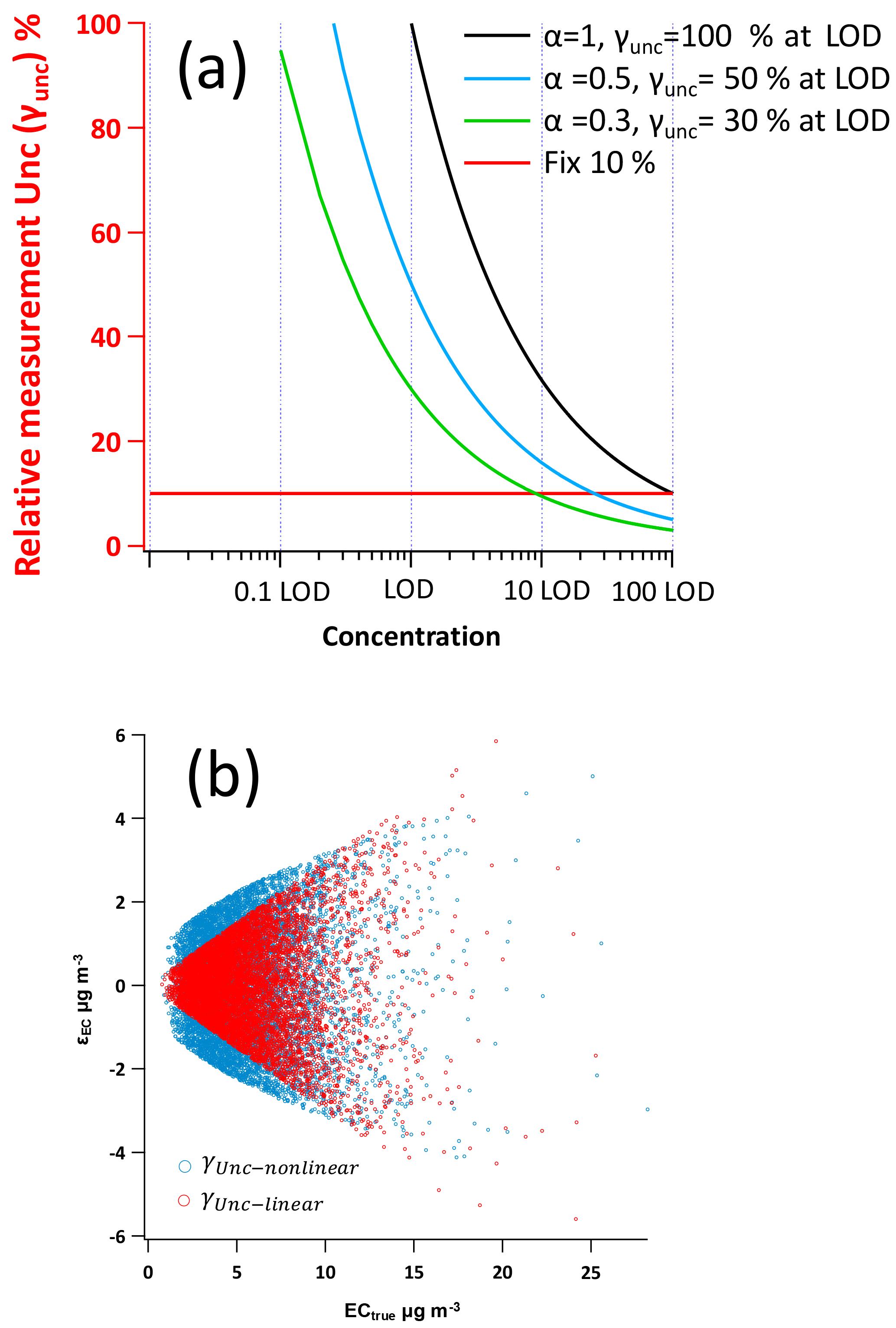
https://www.atmos-meas-tech.net/11/1233/2018/amt-11-1233-2018-f01

Figure 1(a) Example γ_{Unc−nonlinear} curves by different α values (Eq. 17). The x axis is concentration (normalized by LOD) in log scale and the y axis is γ_Unc. Black, blue and green line represents α equal to 1, 0.5 and 0.3, respectively, corresponding to the γ_{Unc−nonlinear} at LOD level equals to 100, 50 and 30 %, respectively. The red line represents γ_Unc−linear of 10 %. (b) Example of measurement uncertainty generation of γ_{Unc−nonlinear} and γ_Unc−linear. The blue circles represent γ_{Unc−nonlinear} following Eq. (17) (LOD_EC=1, a_EC=1). The red circles represent γ_Unc−linear (30 %).

Download

Uniform distribution has been used in previous studies (Cox et al., 2003; Chu, 2005; Saylor et al., 2006) and is adopted in this study to parameterize measurement error. For a uniform distribution in the interval [a,b], the variance is $\frac{1}{12} {(a - b)}^{2}$ . Since ε_POC and ε_EC follow a uniform distribution in the interval as given by Eqs. (18) and (19), the weights in DR and YR (inverse of variance) become

\begin{array}{l} (20) & ω (X_{i}) = \frac{1}{σ_{X_{i}}^{2}} = \frac{3}{{EC}_{true} \times {LOD}_{EC} \times α_{EC}^{2}}, \\ (21) & ω (Y_{i}) = \frac{1}{σ_{Y_{i}}^{2}} = \frac{3}{{POC}_{true} \times {LOD}_{POC} \times α_{POC}^{2}} . \end{array}

The parameter λ in Deming regression is then determined:

\begin{matrix} (22) & λ = \frac{ω (X_{i})}{ω (Y_{i})} = \frac{{POC}_{true} \times {LOD}_{POC} \times α_{POC}^{2}}{{EC}_{true} \times {LOD}_{EC} \times α_{EC}^{2}} . \end{matrix}

Besides the γ_{Unc−nonlinear} discussed above, a second type measurement uncertainty parameterized by a constant proportional factor, γ_Unc−linear, is very common in atmospheric applications:

\begin{array}{l} (23) & - γ_{POCunc} \times {POC}_{true} \leq ε_{POC} \leq + γ_{POCunc} \times {POC}_{true}, \\ (24) & - γ_{ECunc} \times {EC}_{true} \leq ε_{EC} \leq + γ_{ECunc} \times {EC}_{true} . \end{array}

where γ_POCunc and γ_ECunc are the relative measurement uncertainties, e.g., for relative measurement uncertainty of 10 %, γ_Unc= 0.1. As a result, the measurement error is linearly proportional to the concentration. An example comparison of γ_{Unc−nonlinear} and γ_Unc−linear is shown in Fig. 1b. For γ_Unc−linear, the weights become

\begin{array}{l} (25) & ω (X_{i}) = \frac{1}{σ_{X_{i}}^{2}} = \frac{3}{{(γ_{ECunc} \times {EC}_{true})}^{2}}, \\ (26) & ω (Y_{i}) = \frac{1}{σ_{Y_{i}}^{2}} = \frac{3}{{(γ_{POCunc} \times {POC}_{true})}^{2}}, \end{array}

and λ for Deming regression can be determined:

\begin{matrix} (27) & λ = \frac{ω (X_{i})}{ω (Y_{i})} = \frac{{(γ_{POCunc} \times {POC}_{true})}^{2}}{{(γ_{ECunc} \times {EC}_{true})}^{2}} . \end{matrix}

3.1.2 XY data generation by the Mersenne twister generator following a specific distribution

The Mersenne twister (MT) is a pseudorandom number generator (PRNG) developed by Matsumoto and Nishimura (1998). MT has been widely adopted by mainstream numerical analysis software (e.g., MATLAB, SPSS, SAS and Igor Pro) as well as popular programing languages (e.g., R, Python, IDL, C $+ +$ and PHP). Data generation using MT provides a few advantages: (1) frequency distribution can be easily assigned during the data generation process, allowing straightforward simulation of the frequency distribution characteristics (e.g., Gaussian or lognormal) observed in ambient measurements; (2) the inputs for data generation are simply the mean and standard deviation of the data series and can be changed easily by the user; (3) the correlation (R²) between X and Y can be manipulated easily during the data generation to satisfy various purposes; and (4) unlike the sine function described by Chu (2005), which has a sample size limitation of 120, the sample size in MT data generation is highly flexible.

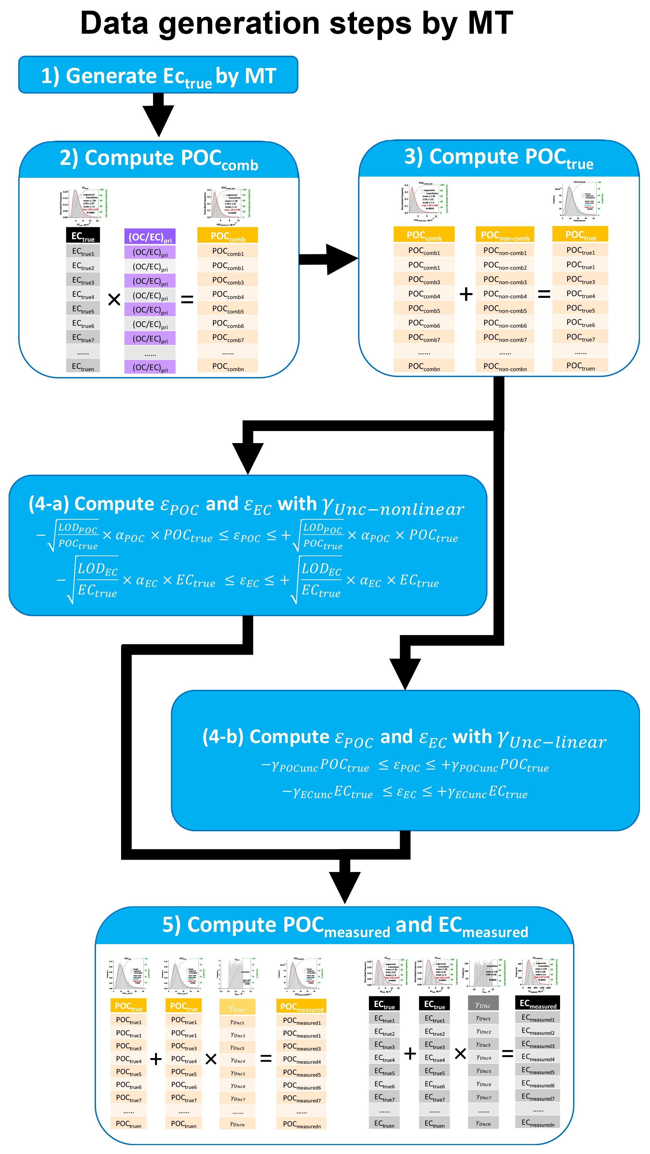
In this section, we will use POC as Y and EC as X as an example to explain the data generation. Procedure of applying MT to simulate ambient POC and EC data can be found in our previous study (Wu and Yu, 2016). Details of the data generation steps are shown in Fig. 2 and described below. The first step is generation of EC_true by MT. In our previous study, it was found that ambient POC and EC data follow a lognormal distribution in various locations of the Pearl River Delta (PRD) region. Therefore, lognormal distributions are adopted during EC_true generation. A range of average concentration and relative standard deviation (RSD) from ambient samples is considered in formulating the lognormal distribution. The second step is to generate POC_comb. As shown in Fig. 2, POC_comb is generated by multiplying EC_true with (OC ∕ EC)_pri. Instead of having a Gaussian distribution, (OC ∕ EC)_pri in this study is a single value, which favors direct comparison between the true value of (OC ∕ EC)_pri and (OC ∕ EC)_pri estimated from the regression slope. The third step is generation of POC_true by adding POC_non-comb onto POC_comb. Instead of having a distribution, POC_non-comb in this study is a single value, which favors direct comparison between the true value of POC_non-comb and POC_non-comb estimated from the regression intercept. The fourth step is to compute ε_POC and ε_EC. As discussed in Sect. 3.1.1, two types of measurement errors are considered for ε_POC and ε_EC calculation: γ_{Unc−nonlinear} and γ_Unc−linear. In the last step, POC_measured and EC_measured are calculated following Eq. (12), i.e., applying measurement errors on POC_true and EC_true. Then POC_measured and EC_measured can be used as Y and X, respectively, to test the performance of various regression techniques. An Igor Pro-based program with a GUI was developed to facilitate the MT data generation for OC and EC. A brief introduction is given in the Supplement.

https://www.atmos-meas-tech.net/11/1233/2018/amt-11-1233-2018-f02

Figure 2Flowchart of data generation steps using MT.

Download

3.1.3 XY data generation by the sine function of Chu (2005)

Besides MT, inclusion of the sine function data generation scheme in this study mainly serves two purposes. First, the sine function scheme was adopted in two previous studies (Chu, 2005; Saylor et al., 2006), the inclusion of this scheme can help to verify whether the codes in Igor for various regression approaches yield the same results from the two previous studies. Second, the crosscheck between results from sine function and MT provides circumstantial evidence that the MT scheme works as expected.

In this section, XY data generation by sine functions is demonstrated using POC as Y and EC as X. There are four steps in POC and EC data generation as shown by the flowchart in Fig. S2. Details are explained as follows. (1) The first step is to generate POC and EC (Chu, 2005):

\begin{array}{l} (28) & {POC}_{comb} = 14 + 12 (\sin (\frac{x}{τ}) + \sin (x - ϕ)), \\ (29) & {EC}_{true} = 3.5 + 3 (\sin (\frac{x}{τ}) + \sin (x - ϕ)), \end{array}

where x is the elapsed hour ( $x = 1, 2, 3 \dots n$ ; n ≤ 120), τ is used to adjust the width of each peak, and ϕ is used to adjust the phase of the sine wave. The constants 14 and 3.5 are used to lift the sine wave to the positive range of the y axis. An example of data generation by the sine functions of Chu (2005) is shown in Fig. 3. Dividing Eq. (28) by Eq. (29) yields a value of 4. In this way the exact relation between POC and EC is defined clearly as (OC ∕ EC)_pri= 4. (2) With POC_comb and EC_true generated, the second step is to add POC_non-comb to POC_comb to compute POC_true. As for POC_non-comb, a single value is assigned and added to all POC following Eq. (10). Then the goodness of the regression intercept can be evaluated by comparing the regressed intercept with preset POC_non-comb. (3) The third step is to compute ε_POC and ε_EC, considering both γ_{Unc−nonlinear} and γ_Unc−linear. (4) The last step is to apply measurement errors on POC_true and EC_true following Eq. (12). Then POC_measured and EC_measured can be used as Y and X, respectively, to evaluate the performance of various regression techniques.

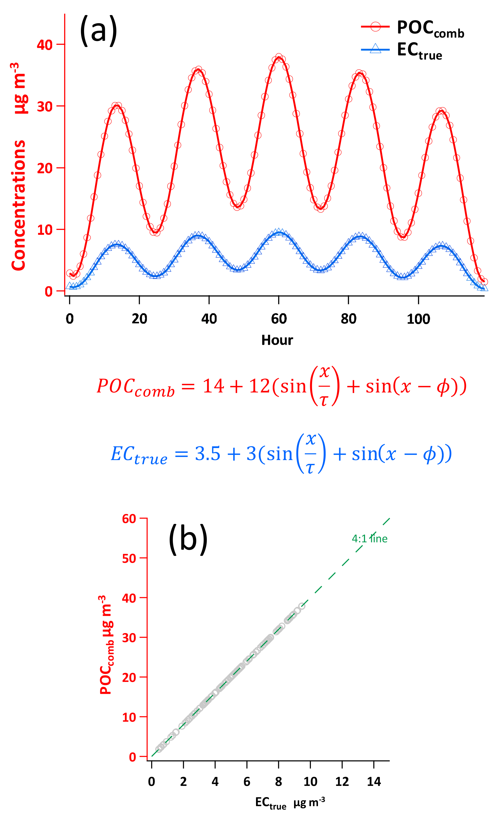
https://www.atmos-meas-tech.net/11/1233/2018/amt-11-1233-2018-f03

Figure 3POC_comb and EC_true data generated by the sine functions of Chu (2005). (a) Time series of the 120 data points for POC_comb and EC_true. (b) Scatter plot of POC_comb vs. EC_true.

Download

3.2 Ambient measurement of σ_abs and EC

Sampling was conducted from Feb 2012 to Jan 2013 at the suburban Nancun (NC) site (23^∘0^′11.82^′′ N, 113^∘21^′18.04^′′ E), which is situated on top of the highest peak (141 m a.s.l.) in the Panyu district of Guangzhou. This site is located at the geographic center of Pearl River Delta region (PRD), making it a good location for representing the average atmospheric mixing characteristics of city clusters in the PRD region. Light absorption measurements were performed by a 7λ Aethalometer (AE-31, Magee Scientific Company, Berkeley, CA, USA). EC mass concentrations were measured by a real time ECOC analyzer (model RT-4, Sunset Laboratory Inc., Tigard, Oregon, USA). Both instruments utilized inlets with a 2.5 µm particle diameter cutoff. The algorithm of Weingartner et al. (2003) was adopted to correct the sampling artifacts (aerosol loading, filter matrix and scattering effect; Collaud Coen et al., 2010) in Aethalometer measurement. A customized computer program with GUI, Aethalometer data processor (Wu et al., 2018), was developed to perform the data correction and detailed descriptions can be found in https://sites.google.com/site/wuchengust. More details of the measurements can be found in Wu et al. (2018).

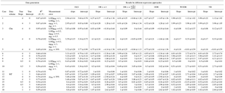
4 Comparison study using synthetic data

In the following comparisons, six regression approaches are compared using two data generation schemes (Chu sine function and MT) separately, as illustrated in Fig. 4. Each data generation scheme considers both γ_{Unc−nonlinear} and γ_Unc−linear in measurement error parameterization. In total, 18 cases are tested with different combination of data generation schemes, measurement error parameterization schemes, true slope and intercept settings. In each case, six regression approaches are tested, i.e., OLS, DR (λ=1), DR $(λ = \frac{ω (X_{i})}{ω (Y_{i})})$ , ODR, WODR and YR. In commercial software (e.g., OriginPro^®, SigmaPlot^®, GraphPad Prism^®), λ in DR is set to 1 by default if not specified. As indicated by Saylor et al. (2006), the bias observed in the study of Chu (2005) is likely due to λ=1 in DR. The purpose of including DR (λ=1) in this study is to examine the potential bias using the default input in many software products. The six regression approaches are considered to examine the sensitivity of regression results to various parameters used in data generation. For each case, 5000 runs are performed to obtain statistically significant results, as recommended by Saylor et al. (2006). The mean slope and intercept from 5000 runs is compared with the true value assigned during data generation. If the difference is < 5 %, the result is considered unbiased.

https://www.atmos-meas-tech.net/11/1233/2018/amt-11-1233-2018-f04

Figure 4Overview of the comparison study design.

Download

4.1 Comparison results using the dataset of Chu (2005)

In this section, the scheme of Chu (2005) is adopted for data generation to obtain a benchmark of six regression approaches. With different setup of slope, intercept and γ_Unc, six cases (Cases 1–6) are studied and the results are discussed below.

Table 1Summary of six regression approaches comparison with 5000 runs for 18 cases.

Download Print Version | Download XLSX

4.1.1 Results with γ_{Unc−nonlinear}

A comparison of the regression techniques results with γ_{Unc−nonlinear} (following Eqs. 18 and 19) is summarized in Table 1. LOD_POC , LOD_EC, α_POC and α_EC are all set to 1 to reproduce the data studied by Chu (2005) and Saylor et al. (2006). Two sets of true slope and intercept are considered (Case 1: slope = 4, intercept = 0; Case 2: slope = 4, intercept = 3) to examine if any results are sensitive to the nonzero intercept. The R² (POC, EC) from 5000 runs for both Case 1 and 2 are 0.67 ± 0.03.

As shown in Fig. 5, for the zero-intercept case (Case 1), OLS significantly underestimates the slope (2.95 ± 0.14), while it overestimates the intercept (5.84 ± 0.78). This result indicates that OLS is not suitable for errors-in-variables linear regression, consistent with similar analysis results from Chu (2005) and Saylor et al. (2006). With DR, if the λ is properly calculated by weights $(λ = \frac{ω (X_{i})}{ω (Y_{i})})$ , unbiased slope (4.01 ± 0.25) and intercept (−0.04 ± 1.28) are obtained; however, results from DR with λ= 1 show obvious bias in the slope (4.27 ± 0.27) and intercept (−1.45 ± 1.36). ODR also produces biased slope (4.27 ± 0.27) and intercept (−1.45 ± 1.36), which are identical to results of DR when λ= 1. With WODR, unbiased slope (3.98 ± 0.22) is observed, but the intercept is overestimated (1.12 ± 1.02). Results of YR are identical to WODR. For Case 2 (slope = 4, intercept = 3), slopes from all six regression approaches are consistent with Case 1 (Table 1). The Case 2 intercepts are equal to the Case 1 intercepts plus 3, implying that all the regression methods are not sensitive to a nonzero intercept.

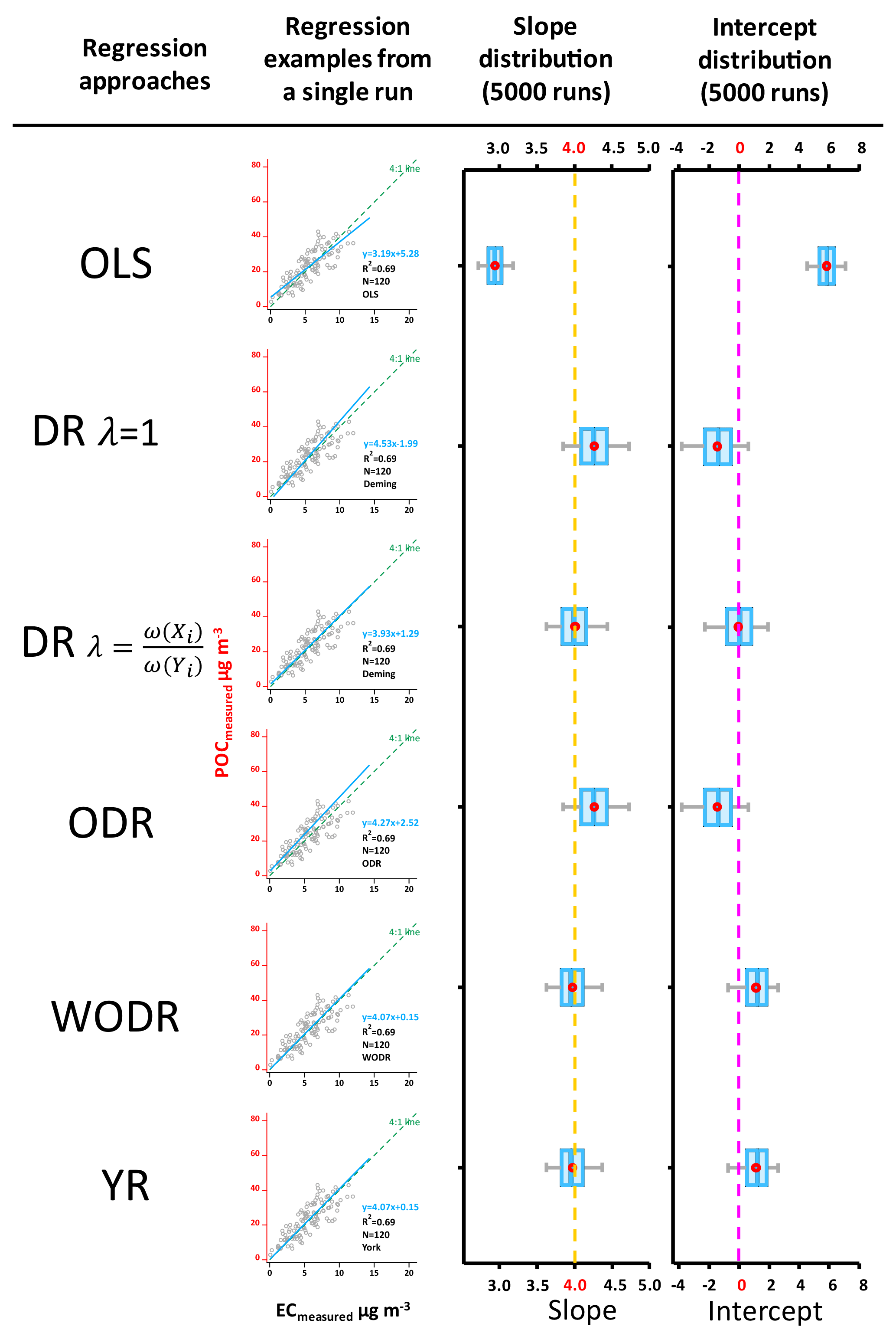
https://www.atmos-meas-tech.net/11/1233/2018/amt-11-1233-2018-f05

Figure 5Regression results on synthetic data, Case 1 (Slope = 4, Intercept = 0, LOD_POC= 1, LOD_EC= 1, a_POC= 1, a_EC= 1, R² (POC, EC) = 0.67 ± 0.03). The scatter plots demonstrate regression examples from a single run. The box plots show the distribution of regressed slopes and intercepts from 5000 runs of six regression approaches. The dashed lines in orange and pink represent true slope and intercept, respectively.

Download

For Case 3, LOD_POC= 0.5, LOD_EC= 0.5, α_POC= 0.5, α_EC= 0.5 are adopted (Table 1), leading to an offset to the left of γ_{Unc−nonlinear} (blue curve) compared to Case 1 and 2 (black curve) in Fig. 1. As a result, for the same concentration of EC and OC in Case 3, the γ_{Unc−nonlinear} is smaller than in Cases 1 and 2 as indicated by a higher R² (0.95 ± 0.01 for Case 3, Table 1). With a smaller measurement uncertainty, the degree of bias in Case 3 is smaller than in Case 1. For example, OLS slope is less biased in Case 3 (3.83 ± 0.08) compared to Case 1 (2.94 ± 0.14). Similarly, the slope (4.03 ± 0.09) and intercept (−0.18 ± 0.44) of DR (λ= 1) exhibit a much smaller bias with a smaller measurement uncertainty, implying that the degree of bias by improperly weighting in DR, WODR and YR is associated with the degree of measurement uncertainty. A higher measurement uncertainty results in larger bias in slope and intercept.

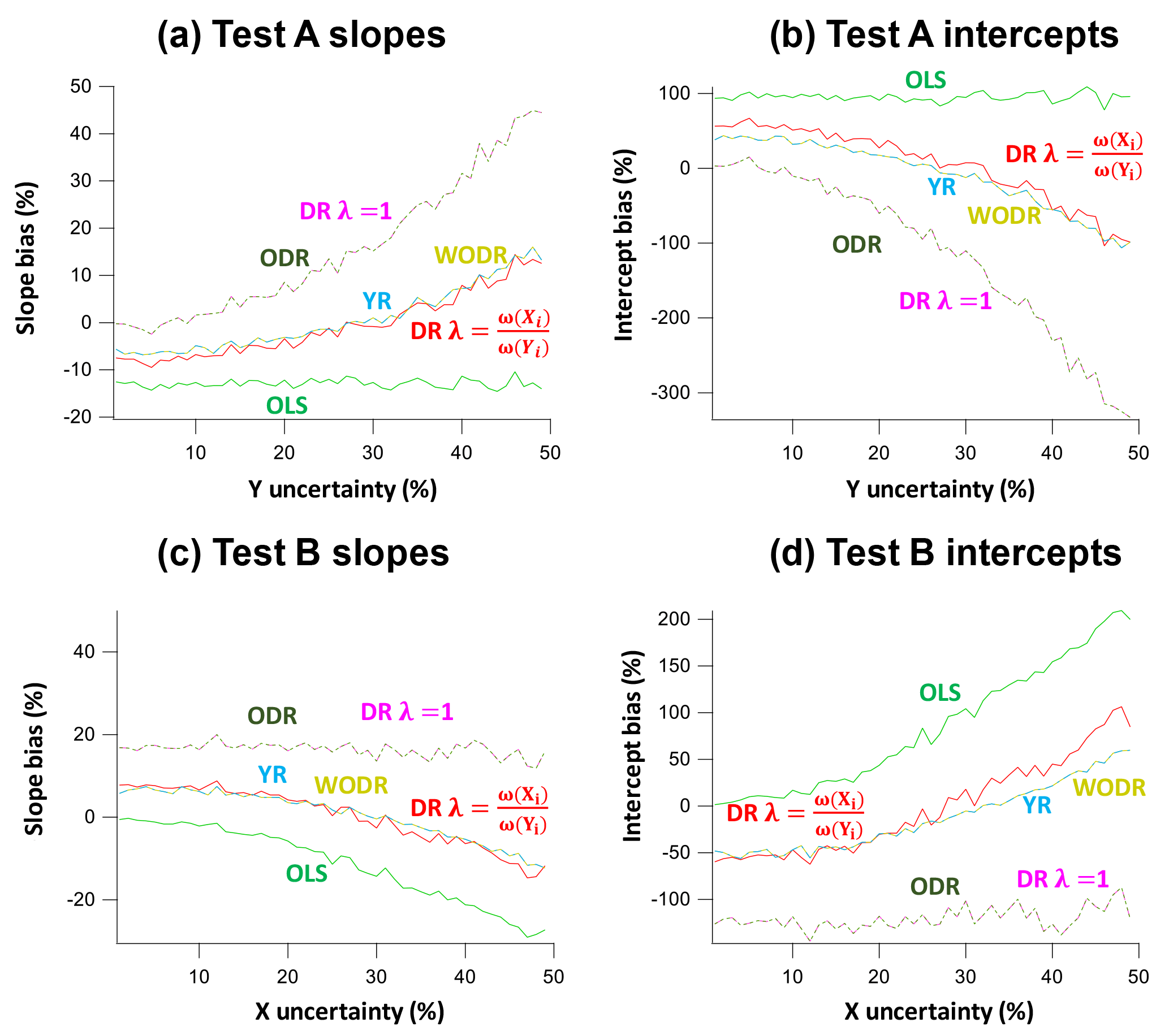
https://www.atmos-meas-tech.net/11/1233/2018/amt-11-1233-2018-f06

Figure 6Slope and intercept biases by different regression schemes in two test scenarios (A and B) in which the assumed error for one of the regression variables deviates from the actual measurement error. In Test A data generation, γ_{Unc_X} is fixed at 30 % and γ_{Unc_Y} is varied between 1 and 50 %. In Test B, γ_{Unc_X} varies between 1 and 50 % and γ_{Unc_Y} is fixed at 30 %. The assumed measurement error for regression is 10 % for both X and Y. (a) Slope biases as a function of γ_{Unc_Y} in Test A. (b) Intercept biases as a function of γ_{Unc_Y} in Test A. (c) Slope biases as a function of γ_{Unc_X} in Test B. (d) Intercept biases as a function of γ_{Unc_X} in Test B.

Download

An uneven LOD_POC and LOD_EC is tested in Case 4 with LOD_POC= 1, LOD_EC= 0.5, α_POC= 0.5, α_EC= 0.5, which yield an R²(POC, EC) of 0.78 ± 0.02. The results are similar to Case 1. For DR $(λ = \frac{ω (X_{i})}{ω (Y_{i})})$ unbiased slope and intercept are obtained. For WODR and YR, unbiased slopes are reported with a small bias in the intercepts. Large bias values are observed in both the slopes and intercepts in Case 4 using OLS, DR (λ=1) and ODR.

4.1.2 Results with γ_Unc−linear

Cases 5 and 6 represent the results from using γ_Unc−linear and are shown in Table 1. γ_Unc is set to 30 % to achieve an R² (POC, EC) of 0.7, a value close to the R² in studies of Chu (2005) and Saylor et al. (2006). In Case 5 (slope = 4, intercept = 0), unbiased slopes and intercepts are determined by DR $(λ = \frac{ω (X_{i})}{ω (Y_{i})})$ , WODR and YR. OLS underestimates the slope (3.32 ± 0.20) and overestimates intercept (3.77 ± 0.90), while DR (λ=1) and ODR overestimate the slopes (4.75 ± 0.30) and underestimate the intercepts (−4.14 ± 1.36). In Case 6 (slope = 4, intercept = 3), results similar to Case 5 are obtained. It is worth noting that although the mean intercept (3.05 ± 1.22) of DR $(λ = \frac{ω (X_{i})}{ω (Y_{i})})$ is closest to the true value (intercept = 3), the deviations are much larger than for WODR (2.72 ± 0.74).

4.2 Comparison results using data generated by MT

In this section, MT is adopted for data generation to obtain a benchmark of six regression approaches. Both γ_{Unc−nonlinear} and γ_Unc−linear are considered. With different configuration of slope, intercept and γ_Unc, 12 cases (Cases 7–18) are studied and the results are discussed below.

4.2.1 γ_{Unc−nonlinear} results

Cases 7 and 8 use data generated by MT and γ_{Unc−nonlinear} with results shown in Table 1. In Case 7 (slope = 4, intercept = 0, LOD_POC= 1, LOD_EC= 1, α_POC= 1, α_EC= 1), unbiased slope (4.00 ± 0.03) and intercept (0.00 ± 0.17) is estimated by DR $(λ = \frac{ω (X_{i})}{ω (Y_{i})})$ . WODR and YR yield unbiased slopes (3.96 ± 0.03) but overestimate the intercepts (1.21 ± 0.13). DR (λ=1) and ODR report slightly biased slopes (4.17 ± 0.04) with biased intercepts (−0.94 ± 0.18). OLS underestimates the slope (3.22 ± 0.03) and overestimates the intercept (4.30 ± 0.14). In Case 8 (slope = 4, intercept = 3, LOD_POC= 1, LOD_EC= 1, α_POC= 1, α_EC= 1), DR $(λ = \frac{ω (X_{i})}{ω (Y_{i})})$ provides unbiased slope (4.00 ± 0.03) and intercept (3.00 ± 0.18) estimations. WODR and YR report unbiased slopes (3.97 ± 0.03) and overestimate intercepts (4.11 ± 0.13). OLS, DR (λ=1) and ODR report biased slopes and intercepts.

To test the overestimation/underestimation dependency on the true slope, Case 9 (slope = 0.5, intercept = 0, LOD_POC= 1, LOD_EC= 1, α_POC= 1, α_EC= 1) and Case 10 (slope = 0.5, intercept = 3, LOD_POC= 1, LOD_EC= 1, α_POC= 1, α_EC= 1) are conducted and the results are shown in Table 1. Unlike the overestimation observed in Cases 1–8, DR (λ=1) and ODR underestimate the slopes (0.46 ± 0.01) in Case 9. In Case 10, DR (λ=1), DR $(λ = \frac{ω (X_{i})}{ω (Y_{i})})$ and ODR report unbiased slopes and intercepts. Cases 11 and 12 test the bias when the true slope is 1, as shown in Table 1. In Case 11 (intercept = 0), all regression approaches except OLS can provide unbiased results. In Case 12, all regression approaches report unbiased slopes except OLS, but DR $(λ = \frac{ω (X_{i})}{ω (Y_{i})})$ is the only regression approach that reports unbiased intercept.

These results imply that if the true slope is less than 1, the improper weighting (λ=1) in Deming regression and ODR without weighting tends to underestimate slope. If the true slope is 1, these two estimators can provide unbiased results. If the true slope is larger than 1, the improper weighting (λ=1) in Deming regression and ODR without weighting tends to overestimate slope.

4.2.2 γ_Unc−linear results

Cases 13 and 14 (Table 1) represent the results from using γ_Unc−linear (30 %) and data generated from MT. For Case 13 (slope = 4, intercept = 0), DR $(λ = \frac{ω (X_{i})}{ω (Y_{i})})$ , WODR and YR provide the best estimation of slopes and intercepts. DR (λ=1) and ODR overestimate slopes (4.53 ± 0.05) and underestimate intercepts (−2.94 ± 0.24). For Case 14 (slope = 4, intercept = 3), DR $(λ = \frac{ω (X_{i})}{ω (Y_{i})})$ , WODR and YR provide an unbiased estimation of slopes. But DR $(λ = \frac{ω (X_{i})}{ω (Y_{i})})$ is the only regression approach reporting unbiased intercept (3.08 ± 0.23). Cases 15 and 16 are tested to investigate whether the results are different if the true slope is smaller than 1. As shown in Table 1, the results are similar to Cases 13 and 14, i.e., that DR $(λ = \frac{ω (X_{i})}{ω (Y_{i})})$ can provide unbiased slope and intercept while WODR and YR can provide unbiased slopes but biased intercepts. Cases 17 and 18 are tested to see if the results are the same for a special case when the true slope is 1. As shown in Table 1, the results are similar to Cases 13 and 14, implying that these results are not sensitive to the special case when the true slope is 1.

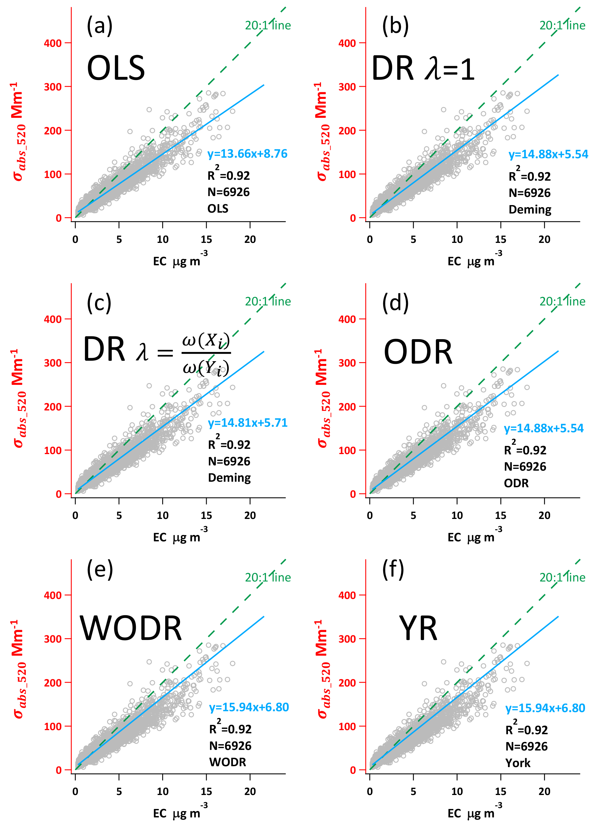
https://www.atmos-meas-tech.net/11/1233/2018/amt-11-1233-2018-f07

Figure 7Regression results using ambient σ_abs520 and EC data from a suburban site in Guangzhou, China.

Download

4.3 The importance of appropriate λ input for Deming regression

As discussed above, inappropriate λ assignment in the Deming regression (e.g., λ= 1 by default for much commercial software) leads to biased slope and intercept. Besides λ= 1, inappropriate λ input due to improper handling of measurement uncertainty can also result in bias for Deming regression. An example is shown in Fig. S3. Data are generated by MT with following parameters: slope = 4, intercept = 0, and γ_Unc−linear (30 %). Figure S2a and b demonstrate that when an appropriate λ is provided (following γ_Unc−linear, $λ = \frac{{POC}^{2}}{{EC}^{2}})$ , unbiased slopes and intercepts are obtained. If an improper λ is used due to a mismatched measurement uncertainty assumption $(γ_{Unc - nonlinear}, λ = \frac{POC}{EC})$ , the slopes are overestimated (Fig. S3c, 4.37 ± 0.05) and intercepts are underestimated (Fig. S3, −2.01 ± 0.24). This result emphasizes the importance of determining the correct form of measurement uncertainty in ambient samples, since λ is a crucial parameter in Deming regression.

In the λ calculation, different representations for POC and EC, including mean, median and mode, are tested as shown in Fig. S4. The results show that when X and Y have a similar distribution (e.g., both are lognormal), any of mean, median or mode can be used for the λ calculation.

4.4 Caveats of regressions with unknown X and Y uncertainties

In atmospheric applications, there are scenarios in which a priori error in one of the variables is unknown, or the measurement error described cannot be trusted. For example, in the case of comparing model prediction and measurement data, the uncertainty of model prediction data is unknown. A second example is the case in which measurement uncertainty cannot be determined due to the lack of duplicated or collocated measurements and as a result, an arbitrarily assumed uncertainty is used. Such a case was illustrated in the study by Flanagan et al. (2006). They found that in the Speciation Trends Network (STN), the whole-system uncertainty retrieved by data from collocated samplers was different from the arbitrarily assumed 5 % uncertainty. Additionally, the discrepancy between the actual uncertainty obtained through collocated samplers and the arbitrarily assumed uncertainty varied by chemical species. To investigate the performance of different regression approaches in these cases, two tests (A and B) are conducted.

In Test A, the actual measurement error for X is fixed at 30 %, while γ_Unc for Y varies from 1 to 50 %. The assumed measurement error for regression is 10 % for both X and Y. Results of Test A are shown in Fig. 6a and b. For OLS, the slopes are underestimated (−14 to −12 %) and intercepts are overestimated (90–103 %) and the biases are independent of variations in γ_{Unc_Y}. ODR and DR (λ=1) yield similar results with overestimated slopes (0–44 %) and underestimated intercepts (−330–0 %). The degree of bias in slopes and intercepts depends on the γ_{Unc_Y}. WODR, DR $(λ = \frac{ω (X_{i})}{ω (Y_{i})})$ and YR perform much better than other regression approaches in Test A, with a smaller bias in both slopes (−8–12 %) and intercepts −98–55 %).

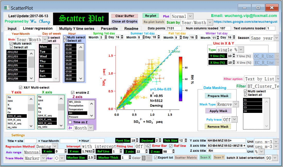
https://www.atmos-meas-tech.net/11/1233/2018/amt-11-1233-2018-f08

Figure 8The user interface of the Scatter Plot Igor program. The program and its operation manual are available from https://doi.org/10.5281/zenodo.832417.

Download

In Test B, γ_{Unc_Y} is fixed at 30 % and γ_{Unc_X} varies between 1 and 50 %. The results of Test B are shown in Fig. 6c and d. The assumed measurement error for regression is 10 % for both X and Y. OLS underestimates the slopes (−29 to −0.2 %) and overestimates the intercepts (2–209 %). In contrast to Test A in which slope and intercept biases are independent of variations in γ_{Unc_Y}, the slope and intercept biases in Test B exhibit dependency on γ_{Unc_X}. The reason for this is that OLS only considers errors in Y and X is assumed to be error-free. ODR and DR (λ=1) yield similar results with overestimated slopes (11–18 %) and underestimated intercepts (−144 to −87 %). The degree of bias in slopes and intercepts is relatively independent on the γ_{Unc_X}. WODR, DR $(λ = \frac{ω (X_{i})}{ω (Y_{i})})$ and YR performed much better than the other regression approaches in Test B, with a smaller bias in both slopes (−14–8 %) and intercepts (−59–106 %).

The results from these two tests suggest that, if one of the measurement errors described cannot be trusted or a priori error in one of the variables is unknown, WODR, DR $(λ = \frac{ω (X_{i})}{ω (Y_{i})})$ and YR should be used instead of ODR and DR (λ=1) and OLS. This conclusion is consistent with results presented in Sect. 4.1 and 4.2. This analysis, albeit crude, also suggests that, in general, the magnitude of bias in slope estimation by these regression approaches is smaller than those for intercept. In other words, slope is a more reliable quantity compared to intercept when extracting quantitative information from linear regressions.

5 Regression applications to ambient data

This section demonstrates the application of the six regression approaches on a light absorption coefficient and EC dataset collected in a suburban site in Guangzhou. As mentioned in Sect. 4.4, measurement uncertainties are crucial inputs for DR, YR and WODR. The measurement precision of Aethalometer is 5 % (Hansen, 2005), while EC by the RT-ECOC analyzer is 24 % (Bauer et al., 2009). These measurement uncertainties are used in DR, YR and WODR calculation. The dataset contains 6926 data points with an R² of 0.92.

As shown in Fig. 7, the y axis is light absorption at 520 nm (σ_abs520) and the x axis is EC mass concentration. The regressed slopes represent the mass absorption efficiency (MAE) of EC at 520 nm, ranging from 13.66 to 15.94 m² g⁻¹ by the six regression approaches. OLS yields the lowest slope (13.66 as shown in Fig. 7a) among all six regression approaches, consistent with the results using synthetic data. This implies that OLS tends to underestimate regression slope when mean Y to X ratio is larger than 1. DR (λ=1) and ODR report the same slope (14.88) and intercept (5.54); this equivalency is also observed for the synthetic data. Similarly, WODR and YR yield identical slope (14.88) and intercept (5.54), in line with the synthetic data results. The regressed slope by DR (λ=1) is higher than DR $(λ = \frac{ω (X_{i})}{ω (Y_{i})})$ , and this relationship agrees well with the synthetic data results.

Regression comparison is also performed on hourly OC and EC data. Regression on OC ∕ EC percentile subset is a widely used empirical approach for primary OC ∕ EC ratio determination. Figure S5 shows the regression slopes as a function of OC ∕ EC percentile. OC ∕ EC percentile ranges from 0.5 to 100 %, with an interval of 0.5 %. As the percentile increases, SOC contribution in OC increases as well, resulting in decreased R² between OC and EC. The deviations between six regression approaches exhibit a dependency on R². When percentile is relatively small (e.g., < 10 %), the differences between the six regression approaches are also small due to the high R² (0.98). The deviations between the six regression approaches become more pronounced as R² decreases (e.g., < 0.9). The deviations are expected to be even larger when R² is less than 0.8. These results emphasize the importance of applying error-in-variables regression, since ambient XY data more likely has an R² less than 0.9 in most cases.

As discussed in this section, the ambient data confirm the results obtained in comparing methods with the synthetic data. The advantage of using the synthetic data for regression approaches evaluation is that the ideal slope and intercept are known values during the data generation, so the bias of each regression approach can be quantified.

6 Recommendations and conclusions

This study aims to provide a benchmark of commonly used linear regression algorithms using a new data generation scheme (MT). Six regression approaches are tested, i.e., OLS, DR (λ=1), DR $(λ = \frac{ω (X_{i})}{ω (Y_{i})})$ , ODR, WODR and YR. The results show that OLS fails to estimate the correct slope and intercept when both X and Y have measurement errors. This result is consistent with previous studies. For ambient data with R² less than 0.9, error-in-variables regression is needed to minimize the biases in slope and intercept. If measurement uncertainties in X and Y are determined during the measurement, measurement uncertainties should be used for regression. With appropriate weighting, DR, WODR and YR can provide the best results among all tested regression techniques. Sensitivity tests also reveal the importance of the weighting parameter λ in DR. An improper λ could lead to biased slope and intercept. Since the λ estimation depends on the form of the measurement errors, it is important to determine the measurement errors during the experimentation stage rather than making assumptions. If measurement errors are not available from the measurement and assumptions are made on measurement errors, DR, WODR and YR are still the best option that can provide the least bias in slope and intercept among all tested regression techniques. For these reasons, DR, WODR and YR are recommended for atmospheric studies when both X and Y data have measurement errors.

Application of error-in-variables regression is often overlooked in atmospheric studies, partly due to the lack of a specified tool for the regression implementation. To facilitate the implementation of error-in-variables regression (including DR, WODR and YR), a computer program (Scatter Plot) with a GUI in Igor Pro (WaveMetrics, Inc. Lake Oswego, OR, USA) was developed (Fig. 8). It is packed with many useful features for data analysis and plotting, including batch plotting, data masking via GUI, color coding in the z axis, data filtering and grouping by numerical values and strings. The Scatter Plot program and user manual are available from https://sites.google.com/site/wuchengust and https://doi.org/10.5281/zenodo.832417.

Data availability

OC, EC and σ_abs data used in this study are available from the corresponding authors upon request. The computer programs used for data analysis and visualization in this study are available in Wu (2017a–c).

Appendix A: Equations of regression techniques

Ordinary least squares (OLS) calculation steps.

First calculate average of observed X_i and Y_i.

\begin{array}{l} (A1) & \overline{X} = \frac{\sum_{i = 1}^{N} X_{i}}{N} \\ (A2) & \overline{Y} = \frac{\sum_{i = 1}^{N} Y_{i}}{N} \end{array}

Then calculate S_xx and S_yy.

\begin{array}{l} (A3) & S_{x x} = \sum_{i = 1}^{N} {(X_{i} - \overline{X})}^{2} \\ (A4) & S_{y y} = \sum_{i = 1}^{N} {(Y_{i} - \overline{Y})}^{2} \end{array}

OLS slope and intercept can be obtained from

\begin{array}{l} (A5) & k = \frac{S_{y y}}{S_{x x}}, \\ (A6) & b = \overline{Y} - k \overline{X} . \end{array}

Deming regression (DR) calculation steps (York, 1966).

Besides S_xx and S_yy as shown above, S_xy can be calculated from

\begin{matrix} (A7) & S_{x y} = \sum_{i = 1}^{N} (X_{i} - \overline{X}) (Y_{i} - \overline{Y}), \end{matrix}

DR slope and intercept can be obtained from

\begin{array}{l} (A8) & k = \frac{S_{y y} - λ S_{x x} + \sqrt{{(S_{y y} - λ S_{x x})}^{2} + 4 λ S_{x y}^{2}}}{2 S_{x y}}, \\ (A9) & b = \overline{Y} - k \overline{X} . \end{array}

York regression (YR) iteration steps (York et al., 2004).

Slope by OLS can be used as the initial k in W_i calculation.

\begin{array}{l} (A10) & W_{i} = \frac{ω (X_{i}) ω (Y_{i})}{ω (X_{i}) + k^{2} ω (Y_{i}) - 2 k r_{i} \sqrt{ω (X_{i}) ω (Y_{i})}} \\ (A11) & U_{i} = X_{i} - \overline{X} = X_{i} - \frac{\sum_{i = 1}^{N} W_{i} X_{i}}{\sum_{i = 1}^{N} W_{i}} \\ (A12) & V_{i} = Y_{i} - \overline{Y} = Y_{i} - \frac{\sum_{i = 1}^{N} W_{i} Y_{i}}{\sum_{i = 1}^{N} W_{i}} \end{array}

Then calculate β_i.

\begin{matrix} (A13) & β_{i} = W_{i} [\frac{U_{i}}{ω (Y_{i})} + \frac{k V_{i}}{ω (X_{i})} - [k U_{i} + V_{i}] \frac{r_{i}}{\sqrt{ω (X_{i}) ω (Y_{i})}}] \end{matrix}

Slope and intercept can be obtained from

\begin{array}{l} (A14) & k = \frac{\sum_{i = 1}^{N} W_{i} β_{i} V_{i}}{\sum_{i = 1}^{N} W_{i} β_{i} U_{i}}, \\ (A15) & b = \overline{Y} - k \overline{X} . \end{array}

Since W_i and β_i are functions of k, k must be solved iteratively by repeating Eqs. (A11) to (A15). If the difference between the k obtained from Eq. (A15) and the k used in Eq. (A11) satisfies the predefined tolerance ( $\frac{k_{i + 1} - k_{i}}{k_{i}} < e^{- 15})$ , the calculation is considered as converged. The calculation is straightforward and usually converged in 10 iterations. For example, the iteration count on the dataset of Chu (2005) is around 6.

Appendix B: Summary of abbreviations and symbols

Abbreviation/symbol	Definition
α	a dimensionless adjustable factor to control the position
	of γ_Unc curve on the concentration axis
b	intercept in linear regression
$β_{i}, U_{i}, V_{i}, W_{i}$	intermediates in York regression calculations
γ_Unc	fractional measurement uncertainties
	relative to the true concentration (%)
DR	Deming regression
ε_EC,ε_POC	absolute measurement uncertainties of EC and POC
EC	elemental carbon
EC_true	numerically synthesized true EC concentration
	without measurement uncertainty
EC_measured	EC with measurement error (EC_true+ε_EC)
λ	ω(X_i) to ω(Y_i)
	ratio in Deming regression
k	slope in linear regression
LOD	limit of detection
MT	Mersenne twister pseudorandom number generator
OC	organic carbon
OC ∕ EC	OC to EC ratio
(OC ∕ EC)_pri	primary OC ∕ EC ratio
OC_non-comb	OC from non-combustion sources
ODR	orthogonal distance regression
OLS	ordinary least squares regression
POC	primary organic carbon
POC_comb	numerically synthesized true POC from combustion
	sources (well correlated with EC_true),
	measurement uncertainty not considered
POC_non-comb	numerically synthesized true POC from non-combustion
	sources (independent of EC_true)
	without considering measurement uncertainty
POC_true	sum of POC_comb and POC_non-comb
	without considering measurement uncertainty
POC_measured	POC with measurement error (POC_true+ε_POC)
$σ_{X_{i}}, σ_{Y_{i}}$	the standard deviation of the error in
	measurement of X_i and Y_i
r_i	correlation coefficient between errors in X_i and Y_i in YR
S	sum of squared residuals
SOC	secondary organic carbon
τ	parameter in the sine function of Chu (2005)
	that adjusts the width of each peak
ϕ	parameter in the sine function of Chu (2005)
	that adjusts the phase of the curve
WODR	weighted orthogonal distance regression
$\overline{X}, \overline{Y}$	average of X_i and Y_i
YR	York regression
ω(X_i),ω(Y_i)	inverse of $σ_{X_{i}}$ and $σ_{Y_{i}}$ ,
	used as weights in DR calculation.

Supplement

The supplement related to this article is available online at: https://doi.org/10.5194/amt-11-1233-2018-supplement.

Competing interests

The authors declare that they have no conflict of interest.

Acknowledgements

This work was supported by the National Natural Science Foundation of China (grant no. 41605002, 41475004 and 21607056), NSFC of Guangdong Province (grant no. 2015A030313339), Guangdong Province Public Interest Research and Capacity Building Special Fund (grant no. 2014B020216005). The author would like to thank Bin Yu Kuang at HKUST for the discussions on mathematics and Stephen M. Griffith at HKUST for the valuable comments.

Edited by: Willy Maenhaut
Reviewed by: two anonymous referees

References

Ayers, G. P.: Comment on regression analysis of air quality data, Atmos. Environ., 35, 2423–2425, https://doi.org/10.1016/S1352-2310(00)00527-6, 2001.

Bauer, J. J., Yu, X.-Y., Cary, R., Laulainen, N., and Berkowitz, C.: Characterization of the sunset semi-continuous carbon aerosol analyzer, J. Air Waste Manage., 59, 826–833, https://doi.org/10.3155/1047-3289.59.7.826, 2009.

Boggs, P. T., Donaldson, J. R., and Schnabel, R. B.: Algorithm 676: ODRPACK: software for weighted orthogonal distance regression, ACM T. Math. Software, 15, 348–364, https://doi.org/10.1145/76909.76913, 1989.

Brauers, T. and Finlayson-Pitts, B. J.: Analysis of relative rate measurements, Int. J. Chem. Kinet., 29, 665–672, https://doi.org/10.1002/(SICI)1097-4601(1997)29:9<665::AID-KIN3>3.0.CO;2-S, 1997.

Cantrell, C. A.: Technical Note: Review of methods for linear least-squares fitting of data and application to atmospheric chemistry problems, Atmos. Chem. Phys., 8, 5477–5487, https://doi.org/10.5194/acp-8-5477-2008, 2008.

Carroll, R. J. and Ruppert, D.: The use and misuse of orthogonal regression in linear errors-in-variables models, Am. Stat., 50, 1–6, https://doi.org/10.1080/00031305.1996.10473533, 1996.

Cess, R. D., Zhang, M. H., Minnis, P., Corsetti, L., Dutton, E. G., Forgan, B. W., Garber, D. P., Gates, W. L., Hack, J. J., Harrison, E. F., Jing, X., Kiehi, J. T., Long, C. N., Morcrette, J.-J., Potter, G. L., Ramanathan, V., Subasilar, B., Whitlock, C. H., Young, D. F., and Zhou, Y.: Absorption of solar radiation by clouds: Observations versus models, Science, 267, 496–499, https://doi.org/10.1126/science.267.5197.496, 1995.

Chen, L. W. A., Doddridge, B. G., Dickerson, R. R., Chow, J. C., Mueller, P. K., Quinn, J., and Butler, W. A.: Seasonal variations in elemental carbon aerosol, carbon monoxide and sulfur dioxide: Implications for sources, Geophys. Res. Lett., 28, 1711–1714, https://doi.org/10.1029/2000GL012354, 2001.

Cheng, Y., Duan, F.-K., He, K.-B., Zheng, M., Du, Z.-Y., Ma, Y.-L., and Tan, J.-H.: Intercomparison of thermal–optical methods for the determination of organic and elemental carbon: influences of aerosol composition and implications, Environ. Sci. Technol., 45, 10117–10123, https://doi.org/10.1021/es202649g, 2011.

Chow, J. C., Watson, J. G., Crow, D., Lowenthal, D. H., and Merrifield, T.: Comparison of IMPROVE and NIOSH carbon measurements, Aerosol. Sci. Technol., 34, 23–34, https://doi.org/10.1080/027868201300081923, 2001.

Chow, J. C., Watson, J. G., Chen, L. W. A., Arnott, W. P., and Moosmuller, H.: Equivalence of elemental carbon by thermal/optical reflectance and transmittance with different temperature protocols, Environ. Sci. Technol., 38, 4414–4422, https://doi.org/10.1021/Es034936u, 2004.

Chu, S. H.: Stable estimate of primary OC ∕ EC ratios in the EC tracer method, Atmos. Environ., 39, 1383–1392, https://doi.org/10.1016/j.atmosenv.2004.11.038, 2005.

Collaud Coen, M., Weingartner, E., Apituley, A., Ceburnis, D., Fierz-Schmidhauser, R., Flentje, H., Henzing, J. S., Jennings, S. G., Moerman, M., Petzold, A., Schmid, O., and Baltensperger, U.: Minimizing light absorption measurement artifacts of the Aethalometer: evaluation of five correction algorithms, Atmos. Meas. Tech., 3, 457–474, https://doi.org/10.5194/amt-3-457-2010, 2010.

Cornbleet, P. J. and Gochman, N.: Incorrect least-squares regression coefficients in method-comparison analysis, Clin. Chem., 25, 432–438, 1979.

Cox, M., Harris, P., and Siebert, B. R.-L.: Evaluation of measurement uncertainty based on the propagation of distributions using Monte Carlo simulation, Meas. Tech., 46, 824–833, https://doi.org/10.1023/B:METE.0000008439.82231.ad, 2003.

Cross, E. S., Onasch, T. B., Ahern, A., Wrobel, W., Slowik, J. G., Olfert, J., Lack, D. A., Massoli, P., Cappa, C. D., Schwarz, J. P., Spackman, J. R., Fahey, D. W., Sedlacek, A., Trimborn, A., Jayne, J. T., Freedman, A., Williams, L. R., Ng, N. L., Mazzoleni, C., Dubey, M., Brem, B., Kok, G., Subramanian, R., Freitag, S., Clarke, A., Thornhill, D., Marr, L. C., Kolb, C. E., Worsnop, D. R., and Davidovits, P.: Soot particle studies – instrument inter-comparison – project overview, Aerosol. Sci. Technol., 44, 592–611, https://doi.org/10.1080/02786826.2010.482113, 2010.

Deming, W. E.: Statistical Adjustment of Data, Wiley, New York, 1943.

Duan, F., Liu, X., Yu, T., and Cachier, H.: Identification and estimate of biomass burning contribution to the urban aerosol organic carbon concentrations in Beijing, Atmos. Environ., 38, 1275–1282, https://doi.org/10.1016/j.atmosenv.2003.11.037, 2004.

Flanagan, J. B., Jayanty, R. K. M., Rickman, J. E. E., and Peterson, M. R.: PM2.5 speciation trends network: evaluation of whole-system uncertainties using data from sites with collocated samplers, J. Air Waste Manage., 56, 492–499, https://doi.org/10.1080/10473289.2006.10464516, 2006.

Hansen, A. D. A.: The Aethalometer manual, Berkeley, California, USA, Magee Scientific, 2005.

Huang, X. H., Bian, Q., Ng, W. M., Louie, P. K., and Yu, J. Z.: Characterization of PM2. 5 major components and source investigation in suburban Hong Kong: A one year monitoring study, Aerosol. Air. Qual. Res., 14, 237–250, https://doi.org/10.4209/aaqr.2013.01.0020, 2014.

Janhäll, S., Andreae, M. O., and Pöschl, U.: Biomass burning aerosol emissions from vegetation fires: particle number and mass emission factors and size distributions, Atmos. Chem. Phys., 10, 1427–1439, https://doi.org/10.5194/acp-10-1427-2010, 2010.

Kuang, B. Y., Lin, P., Huang, X. H. H., and Yu, J. Z.: Sources of humic-like substances in the Pearl River Delta, China: positive matrix factorization analysis of PM^2.5 major components and source markers, Atmos. Chem. Phys., 15, 1995–2008, https://doi.org/10.5194/acp-15-1995-2015, 2015.

Li, Y., Huang, H. X. H., Griffith, S. M., Wu, C., Lau, A. K. H., and Yu, J. Z.: Quantifying the relationship between visibility degradation and PM2.5 constituents at a suburban site in Hong Kong: Differentiating contributions from hydrophilic and hydrophobic organic compounds, Sci. Total Environ., 575, 1571–1581, https://doi.org/10.1016/j.scitotenv.2016.10.082, 2017.

Lim, L. H., Harrison, R. M., and Harrad, S.: The contribution of traffic to atmospheric concentrations of polycyclic aromatic hydrocarbons, Environ. Sci. Technol., 33, 3538–3542, https://doi.org/10.1021/es990392d, 1999.

Lin, P., Hu, M., Deng, Z., Slanina, J., Han, S., Kondo, Y., Takegawa, N., Miyazaki, Y., Zhao, Y., and Sugimoto, N.: Seasonal and diurnal variations of organic carbon in PM2.5 in Beijing and the estimation of secondary organic carbon, J. Geophys. Res., 114, D00G11, https://doi.org/10.1029/2008JD010902, 2009.

Linnet, K.: Necessary sample size for method comparison studies based on regression analysis, Clin. Chem., 45, 882–894, 1999.

Malm, W. C., Sisler, J. F., Huffman, D., Eldred, R. A., and Cahill, T. A.: Spatial and seasonal trends in particle concentration and optical extinction in the United-States, J. Geophys. Res., 99, 1347–1370, https://doi.org/10.1029/93JD02916, 1994.

Markovsky, I. and Van Huffel, S.: Overview of total least-squares methods, Signal Process., 87, 2283–2302, https://doi.org/10.1016/j.sigpro.2007.04.004, 2007.

Matsumoto, M. and Nishimura, T.: Mersenne twister: a 623-dimensionally equidistributed uniform pseudo-random number generator, ACM T. Model. Comput. S., 8, 3–30, https://doi.org/10.1145/272991.272995, 1998.

Moosmüller, H., Arnott, W. P., Rogers, C. F., Chow, J. C., Frazier, C. A., Sherman, L. E., and Dietrich, D. L.: Photoacoustic and filter measurements related to aerosol light absorption during the Northern Front Range Air Quality Study (Colorado 1996/1997), J. Geophys. Res., 103, 28149–28157, https://doi.org/10.1029/98jd02618, 1998.

Petäjä, T., Mauldin III, R. L., Kosciuch, E., McGrath, J., Nieminen, T., Paasonen, P., Boy, M., Adamov, A., Kotiaho, T., and Kulmala, M.: Sulfuric acid and OH concentrations in a boreal forest site, Atmos. Chem. Phys., 9, 7435–7448, https://doi.org/10.5194/acp-9-7435-2009, 2009.

Richter, A., Burrows, J. P., Nusz, H., Granier, C., and Niemeier, U.: Increase in tropospheric nitrogen dioxide over China observed from space, Nature, 437, 129–132, https://doi.org/10.1038/nature04092, 2005.

Saylor, R. D., Edgerton, E. S., and Hartsell, B. E.: Linear regression techniques for use in the EC tracer method of secondary organic aerosol estimation, Atmos. Environ., 40, 7546–7556, https://doi.org/10.1016/j.atmosenv.2006.07.018, 2006.

Thompson, M.: Variation of precision with concentration in an analytical system, Analyst, 113, 1579–1587, https://doi.org/10.1039/AN9881301579, 1988.

Turpin, B. J. and Huntzicker, J. J.: Identification of secondary organic aerosol episodes and quantitation of primary and secondary organic aerosol concentrations during SCAQS, Atmos. Environ., 29, 3527–3544, https://doi.org/10.1016/1352-2310(94)00276-Q, 1995.

von Bobrutzki, K., Braban, C. F., Famulari, D., Jones, S. K., Blackall, T., Smith, T. E. L., Blom, M., Coe, H., Gallagher, M., Ghalaieny, M., McGillen, M. R., Percival, C. J., Whitehead, J. D., Ellis, R., Murphy, J., Mohacsi, A., Pogany, A., Junninen, H., Rantanen, S., Sutton, M. A., and Nemitz, E.: Field inter-comparison of eleven atmospheric ammonia measurement techniques, Atmos. Meas. Tech., 3, 91–112, https://doi.org/10.5194/amt-3-91-2010, 2010.

Wang, J. and Christopher, S. A.: Intercomparison between satellite-derived aerosol optical thickness and PM2.5 mass: Implications for air quality studies, Geophys. Res. Lett., 30, 2095, https://doi.org/10.1029/2003gl018174, 2003.

Watson, J. G.: Visibility: Science and regulation, J. Air Waste Manage., 52, 628–713, https://doi.org/10.1080/10473289.2002.10470813, 2002.

Weingartner, E., Saathoff, H., Schnaiter, M., Streit, N., Bitnar, B., and Baltensperger, U.: Absorption of light by soot particles: determination of the absorption coefficient by means of aethalometers, J. Aerosol. Sci., 34, 1445–1463, https://doi.org/10.1016/S0021-8502(03)00359-8, 2003.

Wu, C.: Scatter Plot, https://doi.org/10.5281/zenodo.832417, 2017a.

Wu, C.: Aethalometer data processor, https://doi.org/10.5281/zenodo.832404, 2017b.

Wu, C.: Histbox, https://doi.org/10.5281/zenodo.832411, 2017c.

Wu, C. and Yu, J. Z.: Determination of primary combustion source organic carbon-to-elemental carbon (OC ∕ EC) ratio using ambient OC and EC measurements: secondary OC-EC correlation minimization method, Atmos. Chem. Phys., 16, 5453–5465, https://doi.org/10.5194/acp-16-5453-2016, 2016.

Wu, C., Ng, W. M., Huang, J., Wu, D., and Yu, J. Z.: Determination of Elemental and Organic Carbon in PM2.5 in the Pearl River Delta Region: Inter-Instrument (Sunset vs. DRI Model 2001 Thermal/Optical Carbon Analyzer) and Inter-Protocol Comparisons (IMPROVE vs. ACE-Asia Protocol), Aerosol. Sci. Technol., 46, 610–621, https://doi.org/10.1080/02786826.2011.649313, 2012.

Wu, C., Huang, X. H. H., Ng, W. M., Griffith, S. M., and Yu, J. Z.: Inter-comparison of NIOSH and IMPROVE protocols for OC and EC determination: implications for inter-protocol data conversion, Atmos. Meas. Tech., 9, 4547–4560, https://doi.org/10.5194/amt-9-4547-2016, 2016.

Wu, C., Wu, D., and Yu, J. Z.: Quantifying black carbon light absorption enhancement with a novel statistical approach, Atmos. Chem. Phys., 18, 289–309, https://doi.org/10.5194/acp-18-289-2018, 2018.

York, D.: Least-squares fitting of a straight line, Can. J. Phys., 44, 1079–1086, https://doi.org/10.1139/p66-090, 1966.

York, D., Evensen, N. M., Martınez, M. L., and Delgado, J. D. B.: Unified equations for the slope, intercept, and standard errors of the best straight line, Am. J. Phys., 72, 367–375, https://doi.org/10.1119/1.1632486, 2004.

Yu, J. Z., Huang, X.-F., Xu, J., and Hu, M.: When Aerosol Sulfate Goes Up, So Does Oxalate: Implication for the Formation Mechanisms of Oxalate, Environ. Sci. Technol., 39, 128–133, https://doi.org/10.1021/es049559f, 2005.

Zhou, Y., Huang, X. H. H., Griffith, S. M., Li, M., Li, L., Zhou, Z., Wu, C., Meng, J., Chan, C. K., Louie, P. K. K., and Yu, J. Z.: A field measurement based scaling approach for quantification of major ions, organic carbon, and elemental carbon using a single particle aerosol mass spectrometer, Atmos. Environ., 143, 300–312, https://doi.org/10.1016/j.atmosenv.2016.08.054, 2016.

Zieger, P., Weingartner, E., Henzing, J., Moerman, M., de Leeuw, G., Mikkilä, J., Ehn, M., Petäjä, T., Clémer, K., van Roozendael, M., Yilmaz, S., Frieß, U., Irie, H., Wagner, T., Shaiganfar, R., Beirle, S., Apituley, A., Wilson, K., and Baltensperger, U.: Comparison of ambient aerosol extinction coefficients obtained from in-situ, MAX-DOAS and LIDAR measurements at Cabauw, Atmos. Chem. Phys., 11, 2603–2624, https://doi.org/10.5194/acp-11-2603-2011, 2011.

Zwolak, J. W., Boggs, P. T., and Watson, L. T.: Algorithm 869: ODRPACK95: A weighted orthogonal distance regression code with bound constraints, ACM T. Math. Software, 33, 27, https://doi.org/10.1145/1268776.1268782, 2007.

Articles

Short summary

A new data generation scheme that employs the Mersenne twister (MT) pseudorandom number generator is proposed to conduct benchmark tests on a variety of linear regression techniques. With an appropriate weighting, Deming regression (DR), weighted ODR (WODR), and York regression (YR) are recommended for atmospheric studies when both x and y data have measurement errors. An Igor-based program (Scatter Plot) is developed to facilitate the regression implementation.

Evaluation of linear regression techniques for atmospheric applications: the importance of appropriate weighting

Ordinary least squares (OLS) method

Orthogonal distance regression (ODR)

Weighted orthogonal distance regression (WODR)

Deming regression (DR)

York regression (YR)

3.1 Synthetic XY data generation

3.1.1 Parameterization of synthesized measurement uncertainty

3.1.2 XY data generation by the Mersenne twister generator following a specific distribution

3.1.3 XY data generation by the sine function of Chu (2005)

3.2 Ambient measurement of σabs and EC

4.1 Comparison results using the dataset of Chu (2005)

4.1.1 Results with γUnc−nonlinear

4.1.2 Results with γUnc−linear

4.2 Comparison results using data generated by MT

4.2.1 γUnc−nonlinear results

4.2.2 γUnc−linear results

4.3 The importance of appropriate λ input for Deming regression

4.4 Caveats of regressions with unknown X and Y uncertainties

3.2 Ambient measurement of σ_abs and EC

4.1.1 Results with γ_{Unc−nonlinear}

4.1.2 Results with γ_Unc−linear

4.2.1 γ_{Unc−nonlinear} results

4.2.2 γ_Unc−linear results