the Creative Commons Attribution 4.0 License.
the Creative Commons Attribution 4.0 License.
 | 06 Mar 2018
Atmospheric QBO and ENSO indices with high vertical resolution from GNSS radio occultation temperature measurements
Hallgeir Wilhelmsen
Florian Ladstädter
Barbara Scherllin-Pirscher
Andrea K. Steiner
We provide atmospheric temperature variability indices for the tropical troposphere and stratosphere based on global navigation satellite system (GNSS) radio occultation (RO) temperature measurements. By exploiting the high vertical resolution and the uniform distribution of the GNSS RO temperature soundings we introduce two approaches, both based on an empirical orthogonal function (EOF) analysis. The first method utilizes the whole vertical and horizontal RO temperature field from 30∘ S to 30∘ N and from 2 to 35 km altitude. The resulting indices, the leading principal components, resemble the well-known patterns of the Quasi-Biennial Oscillation (QBO) and the El Niño–Southern Oscillation (ENSO) in the tropics. They provide some information on the vertical structure; however, they are not vertically resolved. The second method applies the EOF analysis on each altitude level separately and the resulting indices contain information on the horizontal variability at each densely available altitude level. They capture more variability than the indices from the first method and present a mixture of all variability modes contributing at the respective altitude level, including the QBO and ENSO. Compared to commonly used variability indices from QBO winds or ENSO sea surface temperature, these new indices cover the vertical details of the atmospheric variability. Using them as proxies for temperature variability is also of advantage because there is no further need to account for response time lags. Atmospheric variability indices as novel products from RO are expected to be of great benefit for studies on atmospheric dynamics and variability, for climate trend analysis, as well as for climate model evaluation.


Two modes of interannual variability dominate the natural temperature variability in the tropical region: the Quasi-Biennial Oscillation (QBO) and El Niño–Southern Oscillation (ENSO).
In the stratosphere, equatorial zonal wind regimes of easterlies (winds blowing from east) and westerlies propagate downwards at about 1 km month−1. As soon as the westerlies fade out, the easterlies take over, and vice versa. The winds at 10 hPa are out of phase with the winds at 70 hPa. The period of the regimes varies considerably, with an average period of a little more than two years (approximately 28 months), which gives the phenomenon its name, QBO.
There are several characteristics describing the QBO. The two wind regimes do not change much along the longitudinal axis (Naujokat, 1986), but exhibit a distinct latitudinal structure. Strongest QBO-related winds are latitudinally symmetric, centered over the Equator (Dunkerton and Delisi, 1985), and decrease considerably off the Equator with a meridional half width of less than 15∘. The winds are strongest in the middle to lower tropical stratosphere, although the QBO is detectable from the tropopause up to 50 km (Wallace et al., 1993). The atmospheric temperature anomalies are proportional to the vertical gradient of the zonal winds (Randel et al., 1999; Baldwin et al., 2001), which makes it possible to investigate the QBO through temperature anomalies. For a review on QBO features, see Baldwin et al. (2001).
Recently there was a disruption in the stable QBO cycle, where the westerlies took a shortcut upwards, and prevented the easterlies from propagating downwards to the troposphere, as it usually does (Newman et al., 2016; Osprey et al., 2016; Dunkerton, 2017); this also resulted in an anomalous behavior response of trace gases (Tweedy et al., 2017). The causes of this unprecedented disruption in the QBO observational record are still under investigation. Possible explanations include dynamical forcing from waves (Osprey et al., 2016; Coy et al., 2017) or coupling with the 2015/2016 warm ENSO event (Newman et al., 2016; Dunkerton, 2016).
In the troposphere, the dominant interannual variability mode is the ENSO. Its irregular variability originates from a Pacific Ocean–atmosphere interaction and manifests itself as a warm phase (El Niño) and a cold phase (La Niña). Its effects can be detected globally, from the surface to the lower stratosphere (Free and Seidel, 2009; Randel et al., 2009). Commonly the characteristics are described with an ENSO sea surface temperature (SST) index, which can be derived from anomalies in SST in the Niño 3.4 region (5∘ N to 5∘ S and 170 to 120∘ W) of the tropical Pacific. El Niño or La Niña periods are defined to occur if a certain mean SST anomaly threshold is exceeded over several months, e.g., if 5-month running means of SST anomalies in the Niño 3.4 region exceed +0.4 or −0.4 ∘C, respectively, for a minimum of 6 months as defined by Trenberth (1997).
During an El Niño event, there is also warming in the tropical troposphere, with a maximum around 8 km and a cooling in the lowermost stratosphere above the tropopause (Reid, 1994; Randel et al., 2009). There is also an eddy signal, i.e., deviations from the zonal mean (Fernández et al., 2004), with a maximum around 11 km (Scherllin-Pirscher et al., 2012).
The interaction between ENSO and QBO has been investigated in many studies (Taguchi, 2010; Schirber, 2015; Christiansen et al., 2016; Geller et al., 2016; Hansen et al., 2016). For further information on the relationship between ENSO, QBO, and teleconnections, see, e.g., the introduction in Dunkerton (2017) and references within.
Several indices have been introduced to describe the variability of QBO and ENSO in order to better characterize the events, to determine their strength, and to describe their evolution. Trenberth and Stepaniak (2001) suggested the need for a second index, in addition to the Niño 3.4 SST index, to describe the different characteristics of the ENSO-originated variability. Wolter and Timlin (2011) established an extended multivariate ENSO index that is more complete and flexible compared to single-variable ENSO indices.
The QBO is often characterized by wind measurements. Naujokat (1986) established the well-known set of time series from winds at different pressure levels above Singapore. Most frequently used QBO indices are wind anomalies at 30 and 50 hPa pressure levels. Wallace et al. (1993) introduced the representation of the equatorial stratospheric QBO in derived parameters using the leading empirical orthogonal functions of the vertical wind structure.
In this work, we describe a method for creating atmospheric variability indices with high vertical resolution, using global navigation satellite system (GNSS) radio occultation (RO) satellite data.
GNSS RO is a limb sounding technique, where the GNSS signals traverse the Earth's atmosphere and are picked up by receivers at low-Earth orbit (LEO) satellites as they rise or set behind the Earth's horizon relative to the GNSS satellite. On their way to the LEO satellites, the signals are refracted by the atmosphere as they propagate through it. The resulting excess phase path is measured at the LEO satellite. With the help of inversion methods and prior knowledge about the atmosphere, the refraction can be inverted into several atmospheric parameters, one of which is temperature (Melbourne et al., 1994; Kursinski et al., 1997).
The GNSS RO measurements provide vertical atmospheric temperature profiles with a high vertical resolution that are well distributed globally. There have been several RO missions throughout the years, providing data continuously since 2001, and it has been shown that there is no need for calibration between the missions (Schreiner et al., 2007; Foelsche et al., 2011). The greatest-quality GNSS RO measurements are those for the upper troposphere and lower stratosphere region, at about 8 to 35 km in the tropics (Scherllin-Pirscher et al., 2011).
Randel et al. (2003) and Schmidt et al. (2004) showed clear evidence that GNSS RO temperature anomalies can be used for detecting the QBO. This was achieved with only a few years of data in the early phase of the GNSS RO period.
Scherllin-Pirscher et al. (2012) were able to demonstrate that the structure of the ENSO can be detected with GNSS RO temperature anomalies using only 4 years of data. They confirmed the spatial structure of the ENSO during the El Niño events, and showed that the zonal atmospheric response lags SST anomalies by 3 months.
Several other studies have investigated the atmospheric QBO and ENSO signal using GNSS RO data in analyses of climate trends (e.g., Lackner et al., 2011; Steiner et al., 2011) and climate variability (e.g., Randel and Wu, 2015). Teng et al. (2013) and Sun et al. (2014) investigated signatures and characteristics of the ENSO, while Gao et al. (2017) used RO measurements to create an index that describes the strength of the atmospheric response from ENSO and QBO.
We extend this previous work, and use the whole available GNSS RO time series from 2001 to 2017 to create atmospheric variability proxies. We describe the GNSS RO data set in Sect. 2 and explain the applied methods in Sect. 3. Results are presented and discussed in Sect. 4. A summary and conclusions are given in Sect. 5.
We use data from the Wegener Center (WEGC) OPSv5.6 RO multi-satellite record (Schwärz et al., 2016; Angerer et al., 2017) to produce monthly mean gridded temperature fields with a horizontal resolution of 5∘ × 5∘ in longitude and latitude and 200 m vertical resolution. The time period ranges from September 2001 to February 2017.
The WEGC OPSv5.6 data record is a data set with global coverage, but in order to obtain mainly the QBO and ENSO signals, we restrict it to 2 to 35 km altitude and 30∘ S to 30∘ N. At each time step and each altitude level, grid points with missing data are filled horizontally using bilinear interpolation. Our input data set used in this study therefore has Nϕ=12 grid points in latitude (ϕ), Nθ=72 grid points in longitude (θ), Nz=166 grid points in altitude (z), and Nt=186 grid points in time (t).
We create monthly mean temperature anomalies to deseasonalize the data. This is done by calculating the average temperature for each month for the reference time period January 2002 to December 2015. These monthly averages are then subtracted from the original temperature data at the corresponding months. To reduce the month-to-month variations, the monthly mean anomalies are then smoothed with a 1-2-1 running mean filter over time. Finally, time series at each grid point are detrended to avoid any trend in indices of atmospheric variability.
Figure 1 shows zonal mean RO temperature anomalies from 20∘ S to 20∘ N for illustration purposes. We clearly see the downward-propagating QBO pattern in the lower stratosphere, known from previous work, where negative temperature anomalies correspond to westerlies and positive temperature anomalies correspond to easterlies. The highest variability is attributed to the transition from westerlies to easterlies (Scherllin-Pirscher et al., 2017). In the troposphere, we see the variability from the ENSO phenomenon. Several El Niño events are revealed during the GNSS RO time period: during winter 2002–2003, 2004–2005, 2006–2007, and 2009–2010, and during a major event in 2014–2016 that lasted longer than normal (Blunden and Arndt, 2016). The La Niña events 2007–2008, 2010–2011, and 2011–2012 can also be seen.
We create the atmospheric variability indices using two different methods, in the following denoted M1 and M2. They are described in more detail in Sect. 3.1 and 3.2, respectively.
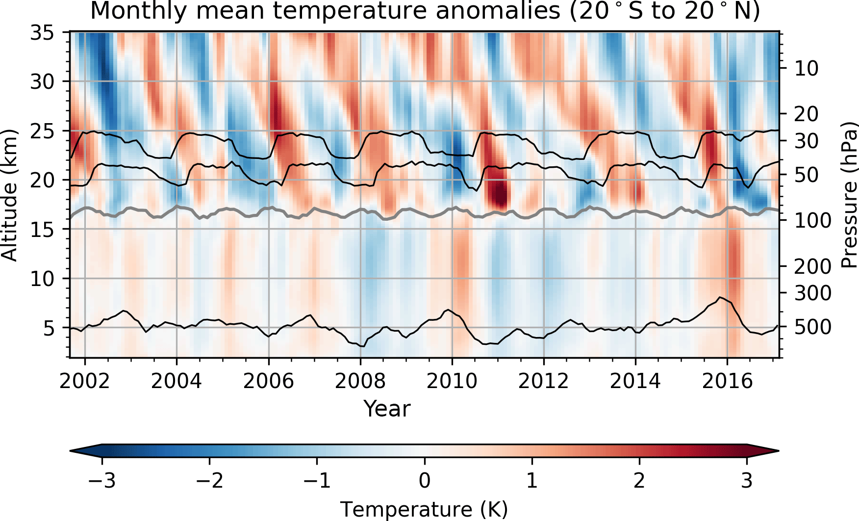
Figure 1Zonal monthly mean temperature anomalies from GNSS RO from 20∘ S to 20∘ N and 2 to 35 km. The gray line near 17 km indicates the tropopause height for the monthly mean temperature profiles, calculated according to the WMO definition of the lapse rate tropopause (WMO, 1957). For illustration, the thinner black lines indicate the conventional QBO30 and QBO50 wind indices (depicted at 30 and 50 hPa, respectively, with arbitrary scale), and the Niño 3.4 SST index (depicted at an arbitrary altitude level with arbitrary scale). The corresponding mean RO pressure levels are indicated on the right y axis. Besides visualizing the features of the QBO in the RO record, they can also be made audible through sonification. Interested readers can hear QBO sounds at https://sysson.iem.at/sounds.html.
In both methods the main variability patterns in the input data set are obtained using an empirical orthogonal function (EOF) analysis. The EOF analysis can extract major modes from spatial and temporal variations. The EOF analysis decomposes the data set into a reduced set of space components and time components (denoted as indices). The first few components will describe most of the variability in descending order of importance (Jolliffe, 2002; Hannachi et al., 2007).
Many names have been used to describe the output from the EOF analysis (see discussion in Wilks, 2006; Hannachi et al., 2007). In the following, we use the terminology from Hannachi et al. (2007), where “EOF” denotes the spatial component, while “PC” denotes the time component. When needed, we use the whole word “principal component” to describe the collection of EOFs, PCs, and eigenvalues.
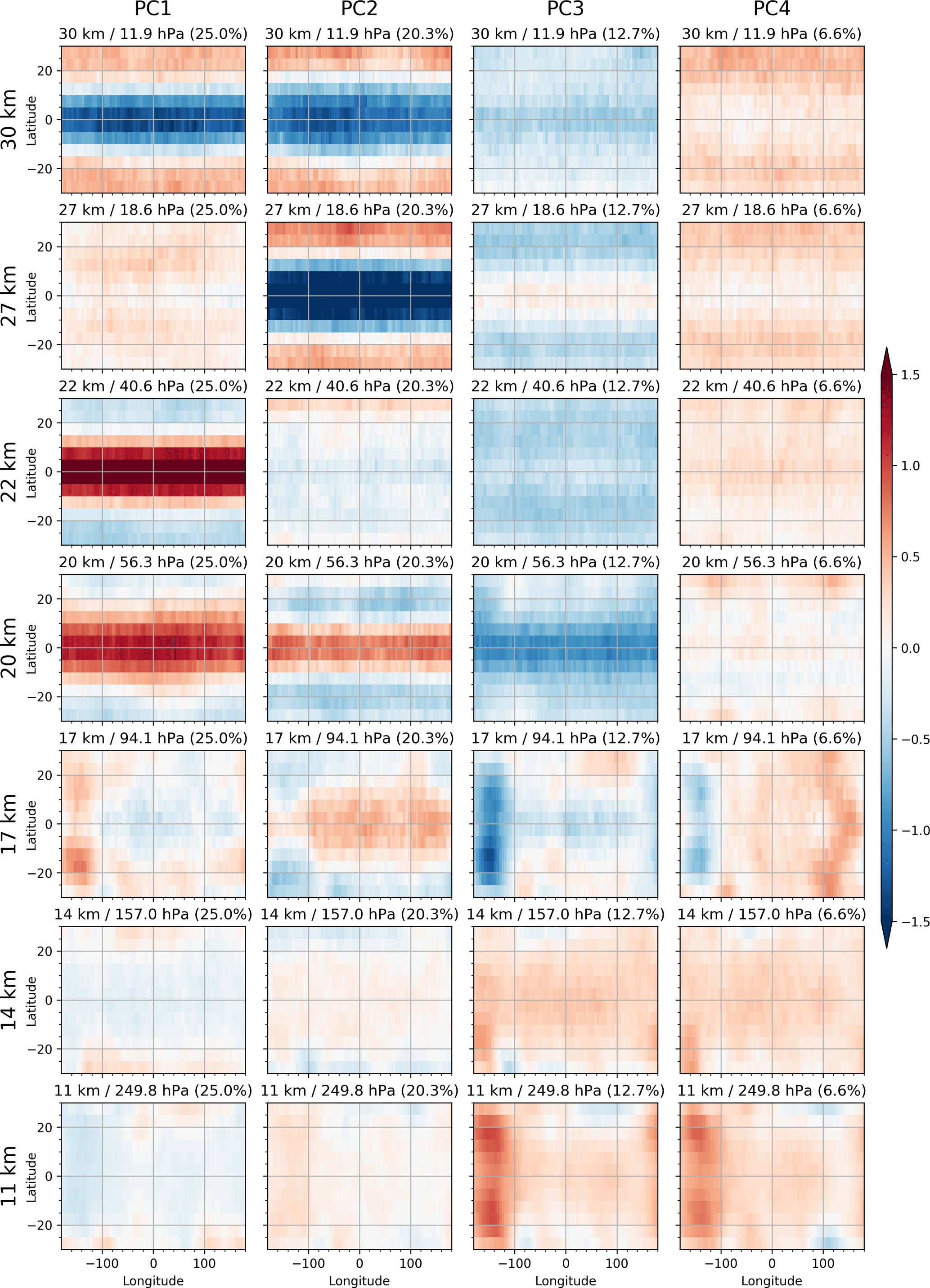
Figure 2The first four EOFs computed from M1, EOF1 to EOF4 (left to right), are shown for selected altitudes at 30, 27, 22, 20, 17, 14, and 11 km (top to bottom). The explained variance ratio is given in parentheses in the titles.
3.1 EOF analysis on the whole temperature field (M1)
In the first method, denoted M1, a space–time matrix is constructed from the monthly mean temperature anomalies described in Sect. 2. The space dimensions are all reshaped into a single axis, (ϕ, θ, z), to reduce the number of dimensions. The resulting matrix is therefore two-dimensional, in space (s) and time (t) only, , represented by Eq. (1), where each row, , corresponds to a time series at a specific location (in ϕ, θ, z).
Each spatial location is denoted with index sp, where p=1…P. Each point in time is denoted tq, where q=1…Q. For M1, using the input data set described in Sect. 2, the spatial direction has the length, . The time dimension has the length Q=186.
The EOF analysis is then based on the decomposition of the covariance matrix (Jolliffe, 2002).
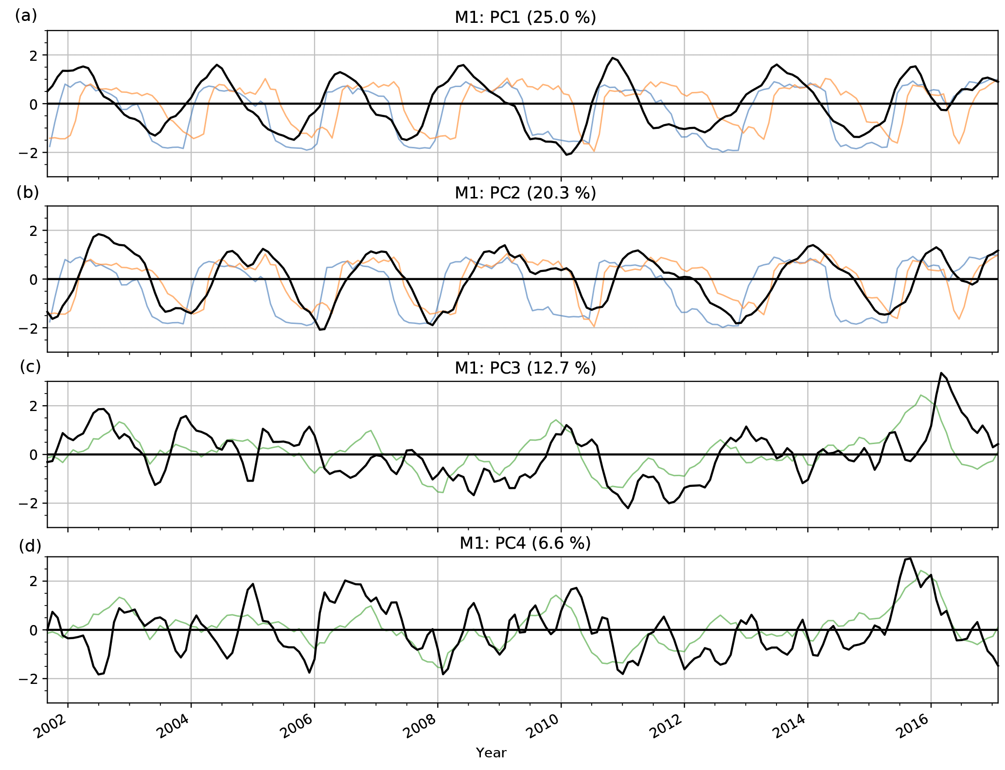
Figure 3The first four PCs computed from M1, PC1 to PC4 (top to bottom, in black). The explained variance ratio is given in parentheses in the titles. For illustration, the conventional QBO wind indices at 30 hPa (blue) and 50 hPa (orange, a, b), and the Niño 3.4 SST index (green, c, d), are indicated on arbitrary scales.
The output of the EOF analysis is a set of EOFs (eigenvectors, in this context called EOFout), PCs (PCout), and their corresponding eigenvalues (λ). The eigenvalues are used to scale the corresponding output EOFs and PCs, according to both Eqs. (2) and (2):
The first few PCs from Eq. (2) can now be used as proxies for the temporal variability. We call these indices in the following. Calculating cross correlations between these indices and conventional indices can hint at their physical interpretation.
3.2 EOF analysis at each altitude level (M2)
To take advantage of the high vertical resolution from RO we also calculate atmospheric variability indices at all altitude levels. In this second method, denoted M2, we do the EOF analysis for each altitude level separately, instead of using the whole field. No altitude-dependent variability is therefore included in the analysis.
To keep the altitude dimension separated from the other dimensions, a space–time matrix is constructed for each altitude level. Therefore, only the latitude and longitude dimensions are reshaped into one axis, leaving us with the space (ϕ, θ) and time (t) dimensions, leading to matrix , which is represented by Eq. (1) at each altitude level, z.
The spatial direction has the length and the time dimension has the length Q=186. The subsequent steps in the EOF analysis are the same as for M1.
The values within each independent EOF show where the principal component contributes to the variability, and how much each point is influenced by its corresponding PC. In the same way, each independent PC shows when the corresponding variability changes.
In this section, we compare the EOFs and PCs constructed from M1 and M2 with characteristics of known atmospheric variability patterns.
4.1 M1 results
The first four resulting EOFs from M1 are presented in Fig. 2. Each EOF has been reshaped to the same space dimensions as the input data set, (ϕ, θ, z). Each column shows an EOF at selected altitude levels.
The spatial structure of the variability from the first and the second EOFs (EOF1 and EOF2, respectively) show characteristics of the QBO. From the stratosphere to the tropopause at around 17 km, the two EOFs do not show distinct longitudinal variability. The patterns are strongest over the Equator with a symmetrical latitudinal dependency, and the tropical band varies with opposite sign to the extratropical latitude band. These features can also be observed with the QBO winds (Naujokat, 1986; Wallace et al., 1993; Baldwin et al., 2001).
EOF1 and EOF2 both exhibit only a weak signal at and below the tropopause, where the pattern also looks different than above.
This longitudinal variability pattern around the tropopause is also visible in the third and the fourth EOFs (EOF3 and EOF4, respectively). The longitudinal pattern disappears at around 14 km where zonal variability dominates. However, it reappears with opposite sign further below at 11 km. This vertical behavior resembles quite well the results of Scherllin-Pirscher et al. (2012), who found a strong eddy ENSO signal with a node at approximately 14 km. This eddy ENSO signal is superimposed with a zonal-mean ENSO signal, which has its node at 17 km.
EOF3 and EOF4 also contribute to the variability above the tropopause. Although the pattern is weak, it is interesting that the signals resemble the patterns of EOF1 and EOF2 above the tropopause.
Figure 3 shows the PC time series (indices) corresponding to the EOFs. The first two PCs, PC1 and PC2, have a regular, sine-wave-like pattern, where one follows the other, with a period of about 2 years. PC3 and PC4 change more rapidly and less regularly.
The output patterns from M1 are not sensitive to the vertical resolution of the input field. We pruned the data to only include every 1 km before performing M1. The EOF pattern looked very much the same as described above, except the PCs showed a coarser pattern, and the explained variances were a little smaller (not shown).
4.2 M2 results
Figure 4 shows the set of the two first EOFs from M2 at the same selected altitude levels as in Fig. 2. Remember that while the EOFs of M1 are functions of latitude, longitude, and altitude, there are separate EOFs for each altitude level resulting from M2. All of these separate EOFs are functions of latitude and longitude only.
The recomposed time series of the two first PCs from M2 are presented in Fig. 5. As for the EOFs, each PC represents an altitude level.
The first set of PCs (Fig. 5a) reveals a separation into a part above the tropopause and into a part below the tropopause. Above the tropopause, the first PCs show the typical downward-propagating QBO pattern. Below the tropopause, the PCs are associated with ENSO events.

Figure 4The first EOFs (left) and second EOFs (right) computed from M2, shown for selected altitude levels from the stratosphere (top) to the troposphere (bottom). The same altitude levels as for Fig. 2 are shown. The explained variance ratio is shown in parentheses in the titles.
The separation at the tropopause can also be seen in Fig. 4. Above the tropopause, the EOF1s from M2 resemble the patterns of either EOF1 or EOF2 of M1 shown in Fig. 2. Above the tropopause the EOF2s also show the same horizontal QBO pattern, though weaker. Below the tropopause, the horizontal patterns of EOF1s and EOF2s resemble EOF3 and EOF4 of M1, which we identified as ENSO-related variability.
The separation is not as clear in the second set of PCs (Fig. 5b). It shows part of the residual variability that is not described by the first set of PCs. These also show downward-propagating patterns, but different from the first set of PCs, and less regular in the stratosphere.
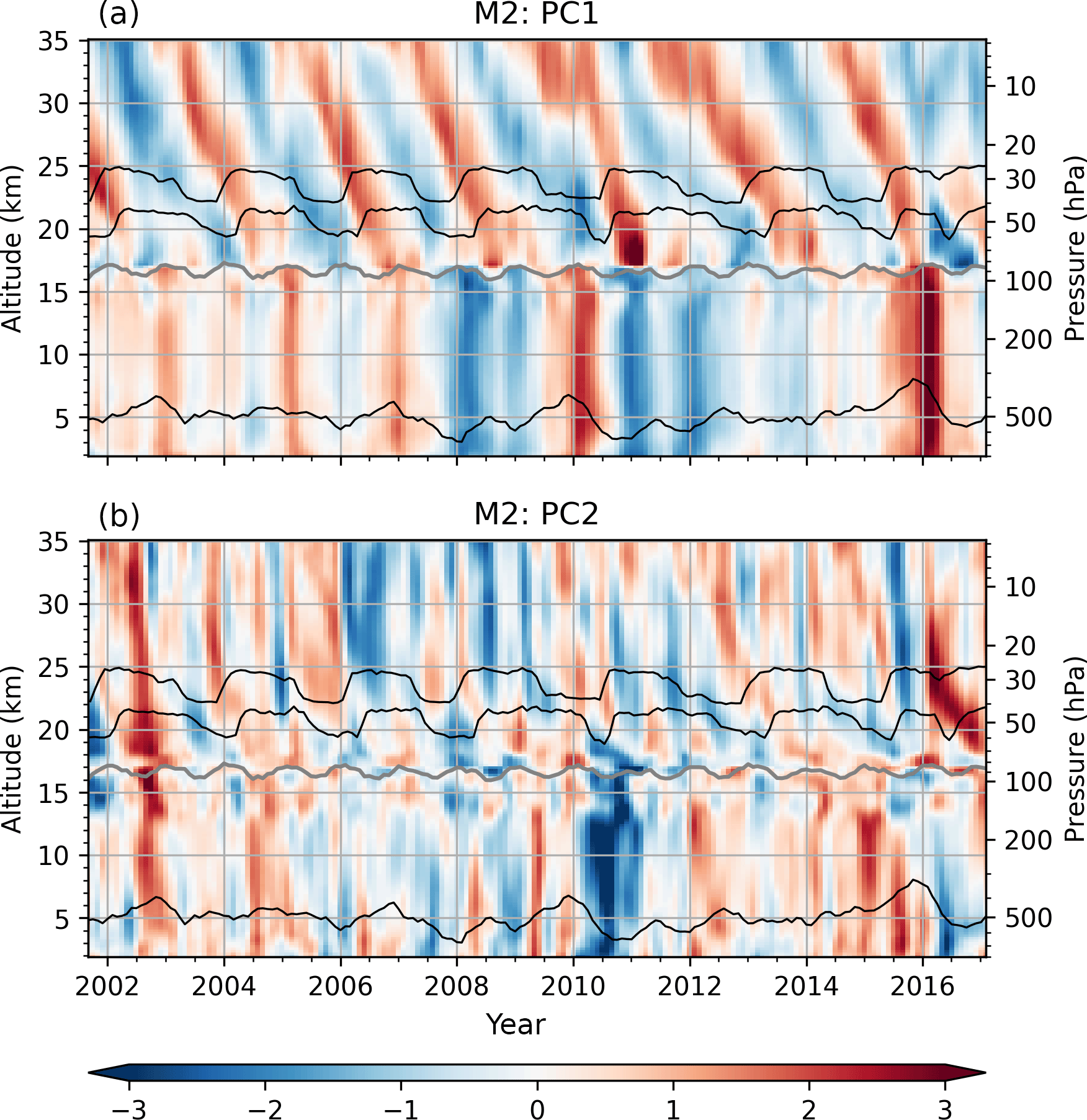
Figure 5PC1s (a) and PC2s (b) from M2 for each altitude level. The gray line indicates the height of the tropopause. For illustration, the thinner black lines indicate the conventional QBO30 and QBO50 wind indices (depicted at 30 and 50 hPa, respectively, with arbitrary scale), and the Niño 3.4 SST index (depicted at an arbitrary altitude level with arbitrary scale).
Keep in mind that both the EOFs and the PCs have been scaled by their corresponding eigenvalues (see Sect. 3.1), at each altitude level separately. The corresponding eigenvalues are proportional to the explained variance ratios (see Fig. 6). The magnitude of each time series therefore does not necessarily describe its importance, nor are the contributions from each EOF or PC directly comparable. The actual contributions can be seen in the reconstruction. See Sect. 4.3 and 4.6 for further details.
Also keep in mind that dominating atmospheric variability at different altitude levels can be caused by different physical mechanisms. The physical context of the first principal components may therefore also change with altitude because the calculations are performed separately at each altitude level for M2. Finally, if independent variability modes explain a similar amount of variance, their corresponding PC time series can switch between two PCs (e.g., between PC1 and PC2) at neighboring altitude levels.
4.3 Explained variance
Figure 6 shows how much each principal component contributes to the total variability. For M1, the first four principal components sum up to 65 % of the total variability (Fig. 6a). Remaining natural variability, associated with, e.g., volcanic eruptions or sudden stratospheric warming events (Randel and Wu, 2015), as well as some remaining sampling issues from GPS RO, account for 35 % of the variance.

Figure 6Explained variance ratio for M1 (a) shown as classical scree plot. Explained variance ratio for M2 (b) shown as a function of altitude for PC1s to PC3s. The dashed lines show the cumulative sums of the explained variance ratios. The horizontal dashed gray line indicates the mean tropopause height.
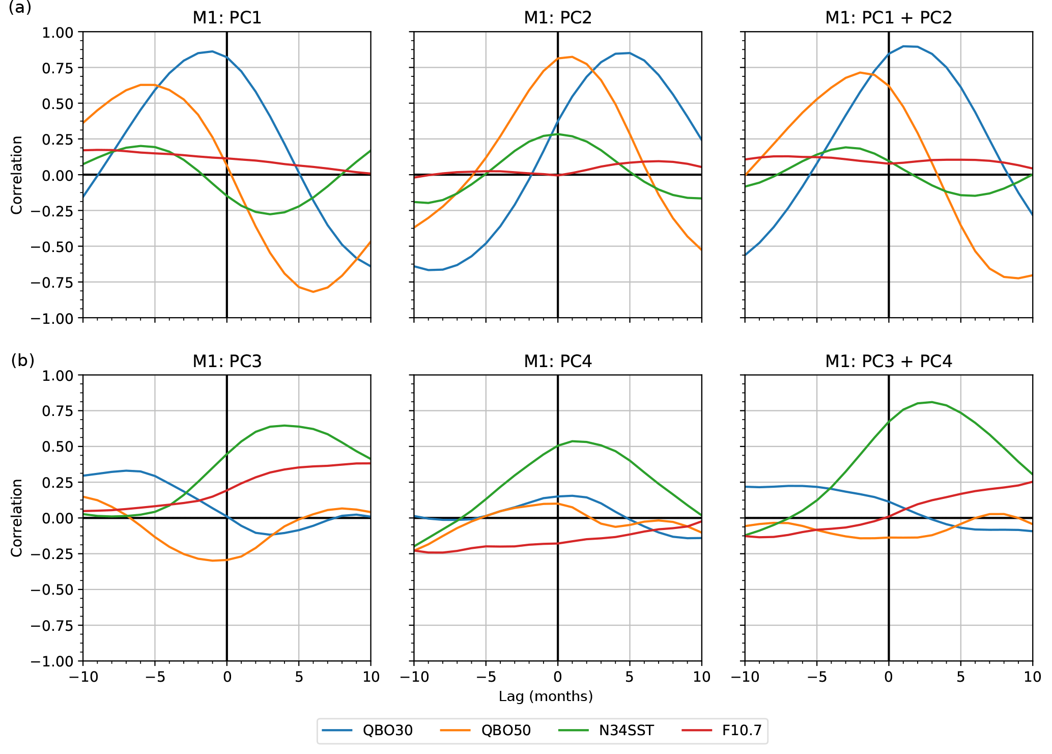
Figure 7Correlations between derived indices (PCs) from M1 with conventional variability indices, QBO30, QBO50, Niño 3.4 SST (N34SST), and F10.7 solar flux (F10.7), shown for ±10-month time lag. Upper panels show PC1, PC2, and PC1 added element-wise to PC2. Lower panels show PC3, PC4, and PC3 added element-wise to PC4.
For M2 (Fig. 6b) the explained variance ratios are shown for the first three principal components at each altitude. Most of the variability is explained by the first principal component, except near the tropopause region, where the first and the second principal components almost touch. In the stratosphere and the troposphere the EOF analysis captures the dominant variability of the QBO and the ENSO, respectively. The tropopause region is less uniform. It is a transition layer between the troposphere and the stratosphere, and more complex in nature (Gettelman and Forster, 2002), possibly explaining the lower explained variance ratio.
4.4 Correlations to conventional indices
In order to show that our deduced indices capture the QBO and ENSO we compute the correlations between the derived PCs and conventional SST and QBO indices.
Figure 7 shows the correlations between the PCs from M1 with the conventional QBO wind indices at 30 hPa (QBO30) and 50 hPa (QBO50), and the Niño 3.4 SST index. The correlations to the solar F10.7 cm flux index are also shown. We do not smooth nor detrend these indices.
We find that both QBO30 and QBO50 correlate well with PC1 alone (top left), and with PC2 alone (top middle), and with PC1 superimposed on (added element-wise to) PC2 (top right). They correlate less well with PC3 alone (bottom left), with PC4 (bottom middle), and with PC3 superimposed with PC4. The time lags are results of the PCs representing the variability at altitudes specified by the EOF patterns. They therefore introduce a time lag when correlating to wind fields at only two pressure levels.
PC3 and PC4 (bottom left and middle) correlate best with the Niño 3.4 SST index. When PC3 is superimposed with PC4 (bottom right), the total correlation to the Niño 3.4 SST index is improved with a time lag of 3 months, known from, e.g., Scherllin-Pirscher et al. (2012).
Figure 8 shows how the PC1s and PC2s derived from M2 correlate with the QBO30 index, QBO50 index, Niño 3.4 SST index, and solar F10.7 cm flux index at each altitude level.
The recomposed set of PC1s correlates well with the QBO30 and QBO50 above the tropopause, and Niño 3.4 SST index below the tropopause, depending on altitude and time lag. There is also some correlation between the set of PC2s to the same indices, although weaker, and without a clear pattern. Both the PC1s and the PC2s have only weak correlation to the solar F10.7 cm flux index.
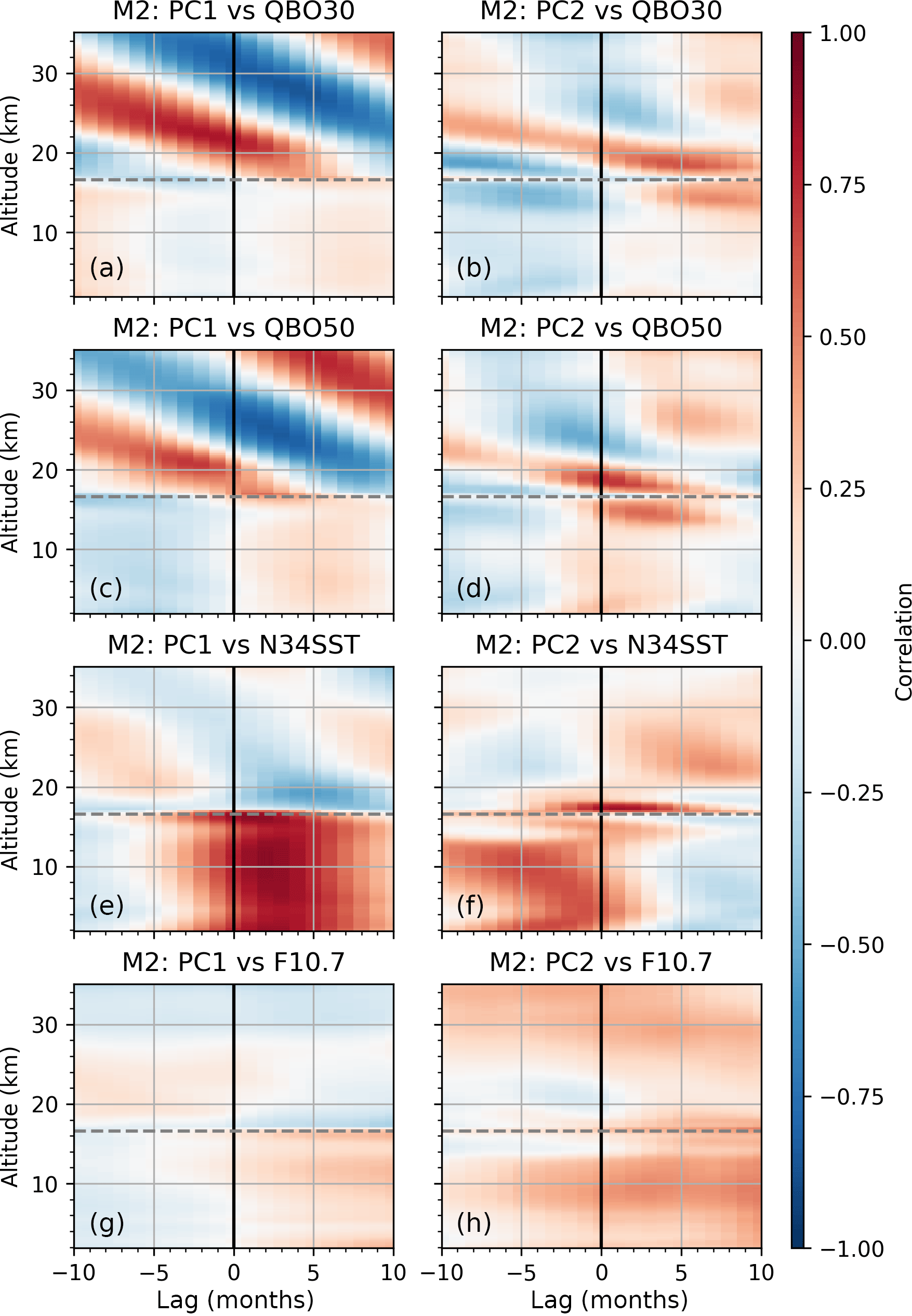
Figure 8Correlations between the first PCs (left) and the second PCs (right) derived from M2 with known variability indices QBO30, QBO50, Niño 3.4 SST (N34SST), F10.7 solar flux (F10.7; top to bottom), shown for each altitude level. The horizontal dashed line indicates the mean tropopause height.
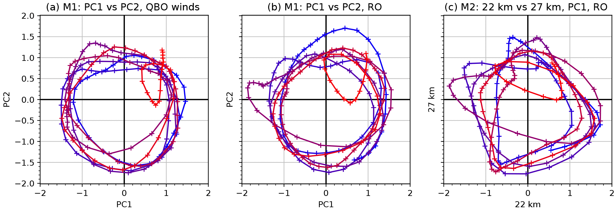
Figure 9Phase space diagrams are shown for the RO time period September 2001 to February 2017. Blue color denotes the beginning of the period and turns into red towards the end of the period. PC1 vs. PC2 from M1 based on QBO winds (a). PC1 vs. PC2 from M1 based on RO temperature (b), and PC1 at 22 km vs. PC1 at 27 km from M2 based on RO temperature (c). For comparison, the PC1 at 27 km (c) is multiplied by −1 to match the orientation of the other panels.
4.5 Phase space diagram
In order to show the relationship between the PCs we present phase space diagrams in Fig. 9, following Fig. 5 in Wallace et al. (1993). Figure 9a shows the relationship between the two first PCs from QBO winds as a trajectory in phase space (PC1 versus PC2). For comparison purposes M1 has been performed using QBO winds at seven pressure levels from 70 to 10 hPa after Wallace et al. (1993). We use the same time period as available in the WEGC OPSv5.6 data set from September 2001 to February 2017. Before plotting we apply a 5-month running mean on the PCs. The resulting phase plot confirms the long history of circularity and nearly constant amplitude of the QBO. The QBO disruption that was observed during 2016 can be clearly seen from the winds (Dunkerton, 2016), and it seems to have found its way back to normal by the end of 2016 (Tweedy et al., 2017).
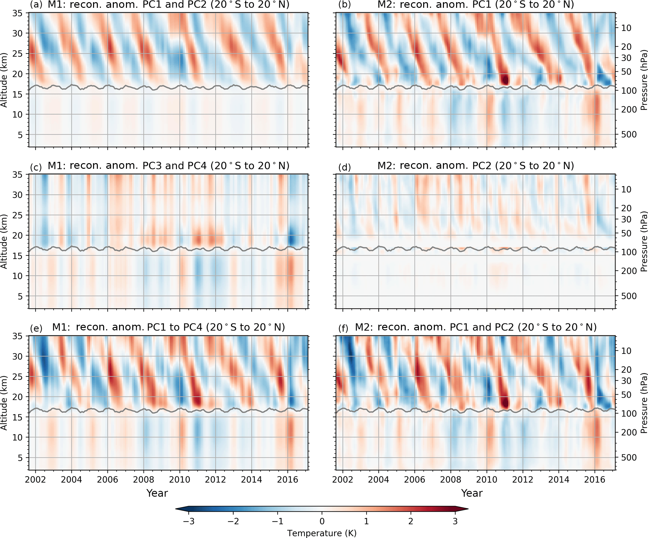
Figure 10Reconstructed temperature fields from the first principal components which explain maximum variability. For M1 (left panels), reconstructed field using PC1 and PC2 (a), PC3 and PC4 (c), and using PC1 to PC4 (e). For M2 (right panels), reconstructed field using the altitude-resolved PC1s (b), using the altitude-resolved PC2s (d), and using PC1s plus PC2s (f). The gray line near 17 km indicates the tropopause height.
Figure 9b shows the same as the left plot, but is constructed from RO temperature anomalies, using PC1 and PC2 from M1 (cf. Fig. 3a, b). It has a similar structure and features as the phase plot from the winds. The QBO disruption is also revealed here, but it has not ended yet in temperature space. This further supports our findings that the main variability obtained by EOF1 and EOF2 from M1 is the QBO.
In Fig. 9c, a phase plot of two PC1s from M2, at two selected altitude levels in the QBO region, is shown. It does not show exactly the same circularity as seen in the two other plots, which could be a result of not covering the same altitude range as in the two other plots. Nevertheless the recent disruption of the QBO can also be seen here.
4.6 Reconstruction of temperature fields
The actual contribution from each principal component to the resulting temperature anomaly field can be seen when reconstructing the principal components. We do this by multiplying the EOF with its corresponding PC (Wilks, 2006). Any scaling by the eigenvalues, or sign flipping, is then canceled out.
Figure 10a shows the reconstructed field using a combination of the first and the second principal components from M1 (see Fig. 3a, b). In contrast to Fig. 5, where the PC1s and the PC2s are plotted in EOF space, we map the PC1s and the PC2s back into anomaly space. We see that most of the contribution to the resulting temperature anomaly field is in the QBO region, which is also expected from the pattern of the EOFs. We clearly see the downward-propagating pattern of the QBO, and only a weak signal in the troposphere. It should be noted that the downward-propagating pattern cannot be created by one principal component alone.
Figure 10c shows the reconstruction using a combination of the third and the fourth principal component from M1 (see Fig. 3c, d). In the troposphere region we see a positive contribution to the temperature field during the El Niño events. The signal right above the tropopause might also be associated with El Niño (e.g., Scherllin-Pirscher et al., 2012), but further up the features seem to be related to the QBO.
Figure 10e shows the reconstruction using all four principal components from M1. This time series well resembles the input temperature anomalies shown in Fig. 1.
For M2, temperature anomaly time series have been reconstructed separately at each altitude level from the resulting principal components. Figure 10b shows the reconstruction using the first principal component of each altitude level (see Fig. 3). The result reveals that much of the features in Fig. 1 are already obtained.
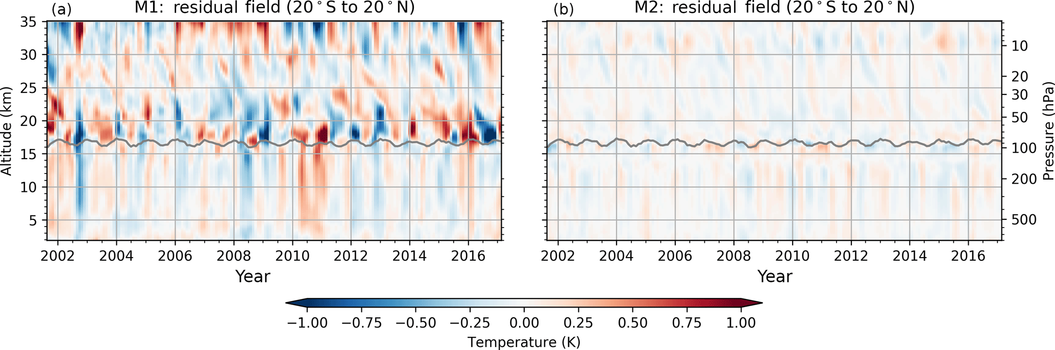
Figure 11The residual temperature field for M1 (a) and M2 (b) showing the difference of the input minus the reconstructed fields, using PC1 to PC4 for M1 and PC1s to PC2s for M2. The gray line near 17 km indicates the tropopause height.
Similarly, Fig. 10d shows the reconstructions from the second principal component for each altitude layer from M2. It describes some features of the variability in the QBO region that are not caught by the first principal component. The stratospheric variability pattern seen in the first principal component (Fig. 10b) seems to find its continuation in the second principal component (Fig. 10d) just above the tropopause.
This suggests that the first principal components are attributable to different variabilities with altitude, and that the attribution can swap between the principal components. It is therefore important to include both indices to catch the variability, especially around the tropopause.
Figure 10f shows a combination of the first and second principal components, and as for M1, it also resembles the input temperature field (cf. Fig. 1) very well.
The resulting difference between the input field (Fig. 1) minus the respective reconstructed fields (Fig. 10, bottom) from M1 and M2 are presented in Fig. 11. This therefore describes the residue of the two methods. For M1 there is still some residue temperature variability left, especially in the tropopause region, but also in the other regions. For M2, however, there is only some minor residue left, especially in the tropopause region. M2 shows a much smaller residue than M1 which indicates that the altitude-resolved indices better capture the atmospheric variability.
Atmospheric variability in the tropical region is often described by indices of the two main modes of variability, the QBO and the ENSO. These indices, commonly derived from stratospheric winds and SST anomalies, do not cover the vertical details. Since they are not derived from atmospheric temperatures, we need to account for a potentially unknown time lag when using them as proxies for atmospheric temperature variability at a specific altitude level.
In this work we introduce new atmospheric variability proxies constructed directly from GNSS RO temperature measurements of high vertical resolution, using standard EOF analysis. We prepared the GNSS RO temperature field for the EOF analysis in two ways.
In the first method, the input field for the EOF analysis includes the whole vertical and horizontal information from 2 to 35 km and from 30∘ S to 30∘ N. The resulting principal components show the well-known characteristics of QBO and ENSO, seen in previous work, and the first four PC time series describe the major part of the variability as a whole. However, they still contain an unknown time lag from the actual variability at different altitude levels, and do not show a strong dependency on the vertical resolution of the input field.
In the second method, we take advantage of the high vertical resolution of GNSS RO and perform an EOF analysis at each altitude level separately to obtain the main horizontal variability at each altitude level. These variability indices, which hold the high vertical resolution from RO, also show the well-known characteristics of the QBO and ENSO, and as they are obtained directly where the variability occurs, they (by their nature) contain no time lag from the actual variability. However, the resulting PCs cannot be attributed to only one or the other mode of variability, but instead present a mixture of all variability modes found at the respective altitude level.
We find that the altitude-resolved indices of the second method capture more of the atmospheric variability than the indices derived from the first method.
Testing the correlation with known classical sea surface temperature indices and wind indices confirmed that the indices derived from RO temperature represent atmospheric variability indices. Further confidence in the results is given as we find the characteristic relationship over time between PC time series from RO temperature consistent with those in winds.
We thus demonstrated that information on the most significant modes of natural climate variability in the tropical troposphere and stratosphere can be derived from GNSS RO temperature observations. Taking advantage of these results, we derive novel products from RO with high added value. Atmospheric variability indices with high vertical resolution can deliver improved information on the natural variability patterns such as QBO and ENSO. Good representation and better knowledge of atmospheric and climate variability is of importance for studies of atmospheric physics and dynamics, the analysis of climate variability and trends, and for the evaluation of climate models.
The WEGC OPSv5.6 RO data set is available on request from the authors and will be made publicly available soon. The QBO wind indices were downloaded from http://www.geo.fu-berlin.de/en/met/ag/strat/produkte/qbo (Freie Universität Berlin, 2018). The Niño 3.4 SST index was downloaded from http://www.cpc.ncep.noaa.gov/data/indices/sstoi.indices (NOAA, 2018a). The solar F10.7 cm flux indices were downloaded from ftp://ftp.ngdc.noaa.gov/STP/space-weather/solar-data/solar-features/solar-radio/noontime-flux/penticton/penticton_observed/listings/listing_drao_noontime-flux-observed_monthly.txt (NOAA, 2018b).
The depicted PCs carry an arbitrary sign that comes from the nature of the EOF analysis method. As we, for M2, perform an EOF analysis independently at each altitude level, the sign of the EOFs and PCs can make sudden changes between the altitude layers. It does not affect the reconstruction, as the sign is simply canceled out in a reconstruction, but it results in a hashed image when visualized as in Fig. 5. To avoid this, we take the following steps.
First, the top altitude layer is chosen as the first basis for the PC direction, PCb (b denotes “basis”). Then, the following steps are performed, for each altitude layer, in descending order:
-
If PCb correlates negatively to the PC at the altitude level i (PCi), the signs of both EOFi and the PCi are flipped (multiplied by −1).
-
The PCb is updated with the resulting PCi, according to
and used as basis for the next altitude layer.
The factor α can take values between 0 and 1. Using α=0.3 seemed to work well for us. PCb is updated no matter if sign flipping takes place or not. It is therefore only used for holding information about the previous PCs, with fading influence with distance to the previous altitude layer.
This is done for all principal components in the resulting data set. It creates much smoother results, without sudden sign changes.
HW performed the computational implementation and the analysis, created the figures, and wrote the first draft of the paper. All authors contributed to the study design. FL provided advice on the analysis design and made major contributions to the text. BSP provided advice on the method and interpretation of the results, and contributed to the text. AKS provided guidance and advice on all aspects of the study, and contributed to the text.
The authors declare that they have no conflict of interest.
This article is part of the special issue “Observing Atmosphere and Climate with Occultation Techniques – Results from the OPAC-IROWG 2016 Workshop”. It is a result of the International Workshop on Occultations for Probing Atmosphere and Climate, Leibnitz, Austria, 8–14 September 2016.
We are grateful to UCAR/CDAAC (Boulder, CO, USA) for provision of
RO phase and orbit data and to ECMWF (Reading, UK) for providing access
to analysis and forecast data. The WEGC processing team members
(Marc Schwärz, Barbara Angerer) are thanked for providing the OPSv5.6 RO
data. We acknowledge FU Berlin (Berlin, DE) for providing QBO wind
indices, CPC for ENSO indices, and NOAA for the solar flux indices. We
thank Harald Rieder (WEGC, AT), Thomas Mendlik (WEGC, AT), and Alejandro de la Torre
(Universidad Austral, AR) for their help and fruitful discussion. This
work was funded by the Austrian Science Fund (FWF) under research grants
P27724-NBL (VERTICLIM) and W1256-G15 (Doctoral Programme Climate Change
– Uncertainties, Thresholds and Coping Strategies).
Edited by: Anthony Mannucci
Reviewed by: five anonymous referees
Angerer, B., Ladstädter, F., Scherllin-Pirscher, B., Schwärz, M., Steiner, A. K., Foelsche, U., and Kirchengast, G.: Quality aspects of the Wegener Center multi-satellite GPS radio occultation record OPSv5.6, Atmos. Meas. Tech., 10, 4845–4863, https://doi.org/10.5194/amt-10-4845-2017, 2017. a
Baldwin, M. P., Gray, L. J., Dunkerton, T. J., Hamilton, K., Haynes, P. H., Randel, W. J., Holton, J. R., Alexander, M. J., Hirota, I., Horinouchi, T., Jones, D. B. A., Kinnersley, J. S., Marquardt, C., Sato, K., and Takahashi, M.: The Quasi-Biennial Oscillation, Rev. Geophys., 39, 179–229, 2001. a, b, c
Blunden, J. and Arndt, D. S.: State of the Climate in 2015, B. Am. Meteorol. Soc., 97, Si–S275, https://doi.org/10.1175/2016BAMSStateoftheClimate.1, 2016. a
Christiansen, B., Yang, S., and Madsen, M. S.: Do strong warm ENSO events control the phase of the stratospheric QBO?, Geophys. Res. Lett., 43, 10489–10495, https://doi.org/10.1002/2016GL070751, 2016. a
Coy, L., Newman, P. A., Pawson, S., and Lait, L. R.: Dynamics of the Disrupted 2015/16 Quasi-Biennial Oscillation, J. Climate, 30, 5661–5674, https://doi.org/10.1175/JCLI-D-16-0663.1, 2017. a
Dunkerton, T. J.: The quasi-biennial oscillation of 2015–2016: Hiccup or death spiral?, Geophys. Res. Lett., 43, 10547–10552, https://doi.org/10.1002/2016GL070921, 2016. a, b
Dunkerton, T. J.: Nearly identical cycles of the quasi-biennial oscillation in the equatorial lower stratosphere, J. Geophys. Res.-Atmos, 122, 8467–8493, https://doi.org/10.1002/2017JD026542, 2017. a, b
Dunkerton, T. J. and Delisi, D. P.: Climatology of the Equatorial Lower Stratosphere, J. Atmos. Sci., 42, 376–396, https://doi.org/10.1175/1520-0469(1985)042<0376:COTELS>2.0.CO;2, 1985. a
Fernández, N. C., García, R. R., Herrera, R. G., Puyol, D. G., Presa, L. G., Martín, E. H., and Rodríguez, P. R.: Analysis of the ENSO signal in tropospheric and stratospheric temperatures observed by MSU, 1979–2000, J. Climate, 17, 3934–3946, 2004. a
Foelsche, U., Scherllin-Pirscher, B., Ladstädter, F., Steiner, A. K., and Kirchengast, G.: Refractivity and temperature climate records from multiple radio occultation satellites consistent within 0.05 %, Atmos. Meas. Tech., 4, 2007–2018, https://doi.org/10.5194/amt-4-2007-2011, 2011. a
Free, M. and Seidel, D. J.: Observed El Niño–Southern Oscillation temperature signal in the stratosphere, J. Geophys. Res., 114, D23108, https://doi.org/10.1029/2009JD012420, 2009. a
Freie Universität Berlin: The Quasi-Biennial-Oscillation (QBO) Data Serie, available at: http://www.geo.fu-berlin.de/en/met/ag/strat/produkte/qbo, last access: 22 February 2018. a
Gao, P., Xu, X., and Zhang, X.: On the relationship between the QBO/ENSO and atmospheric temperature using COSMIC radio occultation data, J. Atmos. Sol.-Terr. Phy., 156, 103–110, https://doi.org/10.1016/j.jastp.2017.03.008, 2017. a
Geller, M. A., Zhou, T., and Yuan, W.: The QBO, gravity waves forced by tropical convection, and ENSO, J. Geophys. Res.-Atmos, 121, 8886–8895, https://doi.org/10.1002/2015JD024125, 2016. a
Gettelman, A. and Forster, P.: A climatology of the tropical tropopause layer, J. Meteor. Soc. Jpn., 80, 911–924, 2002. a
Hannachi, A., Jolliffe, I. T., and Stephenson, D. B.: Empirical orthogonal functions and related techniques in atmospheric science: A review, Int. J. Climatol., 27, 1119–1152, https://doi.org/10.1002/joc.1499, 2007. a, b, c
Hansen, F., Matthes, K., and Wahl, S.: Tropospheric QBO–ENSO interactions and differences between the Atlantic and Pacific, J. Climate, 29, 1353–1368, https://doi.org/10.1175/JCLI-D-15-0164.1, 2016. a
Jolliffe, I. T.: Principal Component Analysis, Springer Series in Statistics, Springer, https://doi.org/10.1007/b98835, 2002. a, b
Kursinski, E. R., Hajj, G. A., Schofield, J. T., Linfield, R. P., and Hardy, K. R.: Observing Earth's atmosphere with radio occultation measurements using the Global Positioning System, J. Geophys. Res., 102, 23429–23465, https://doi.org/10.1029/97JD01569, 1997. a
Lackner, B. C., Steiner, A. K., Kirchengast, G., and Hegerl, G. C.: Atmospheric Climate Change Detection by Radio Occultation Data Using a Fingerprinting Method, J. Climate, 24, 5275–5291, https://doi.org/10.1175/2011JCLI3966.1, 2011. a
Melbourne, W. G., Davis, E. S., Duncan, C. B., Hajj, G. A., Hardy, K. R., Kursinski, E. R., Meehan, T. K., Young, L. E., and Yunck, T. P.: The application of spaceborne GPS to atmospheric limb sounding and global change monitoring, Tech. rep., Jet Propulsion Laboratory, NASA, Pasadena, California, USA, 1994. a
National Oceanic and Atmospheric Administration (NOAA): Monthly OISST.v2, available at: http://www.cpc.ncep.noaa.gov/data/indices/sstoi.indices, last access: 22 February 2018a. a
National Oceanic and Atmospheric Administration (NOAA): Solar Flux (10.7cm), available at: ftp://ftp.ngdc.noaa.gov/STP/space-weather/solar-data/solar-features/solar-radio/noontime-flux/penticton/penticton_observed/listings/listing_drao_noontime-flux-observed_monthly.txt, last access: 22 February 2018b. a
Naujokat, B.: An Update of the Observed Quasi-Biennial Oscillation of the Stratospheric Winds over the Tropics, J. Atmos. Sci., 43, 1873–1877, https://doi.org/10.1175/1520-0469(1986)043<1873:AUOTOQ>2.0.CO;2, 1986. a, b, c
Newman, P. A., Coy, L., Pawson, S., and Lait, L. R.: The anomalous change in the QBO in 2015–2016, Geophys. Res. Lett., 43, 8791–8797, https://doi.org/10.1002/2016GL070373, 2016. a, b
Osprey, S. M., Butchart, N., Knight, J. R., Scaife, A. A., Hamilton, K., Anstey, J. A., Schenzinger, V., and Zhang, C.: An unexpected disruption of the atmospheric quasi-biennial oscillation, Science, 353, 1424–1427, https://doi.org/10.1126/science.aah4156, 2016. a, b
Randel, W. J. and Wu, F.: Variability of Zonal Mean Tropical Temperatures Derived from a Decade of GPS Radio Occultation Data, J. Atmos. Sci., 72, 1261–1275, https://doi.org/10.1175/JAS-D-14-0216.1, 2015. a, b
Randel, W. J., Wu, F., Swinbank, R., Nash, J., and O'Neill, A.: Global QBO circulation derived from UKMO stratospheric analyses, J. Atmos. Sci., 56, 457–474, 1999. a
Randel, W. J., Wu, F., and Rivera Ríos, W.: Thermal variability of the tropical tropopause region derived from GPS/MET observations, J. Geophys. Res., 108, 4024, https://doi.org/10.1029/2002JD002595, 2003. a
Randel, W. J., Garcia, R. R., Calvo, N., and Marsh, D.: ENSO influence on zonal mean temperature and ozone in the tropical lower stratosphere, J. Geophys. Res., 36, L15822, https://doi.org/10.1029/2009GL039343, 2009. a, b
Reid, G. C.: Seasonal and interannual temperature variations in the tropical stratosphere, J. Geophys. Res., 99, 18923–18932, 1994. a
Scherllin-Pirscher, B., Steiner, A. K., Kirchengast, G., Kuo, Y.-H., and Foelsche, U.: Empirical analysis and modeling of errors of atmospheric profiles from GPS radio occultation, Atmos. Meas. Tech., 4, 1875–1890, https://doi.org/10.5194/amt-4-1875-2011, 2011. a
Scherllin-Pirscher, B., Deser, C., Ho, S.-P., Chou, C., Randel, W., and Kuo, Y.-H.: The vertical and spatial structure of ENSO in the upper troposphere and lower stratosphere from GPS radio occultation measurements, Geophys. Res. Lett., 39, L20801, https://doi.org/10.1029/2012GL053071, 2012. a, b, c, d, e
Scherllin-Pirscher, B., Randel, W. J., and Kim, J.: Tropical temperature variability and Kelvin-wave activity in the UTLS from GPS RO measurements, Atmos. Chem. Phys., 17, 793–806, https://doi.org/10.5194/acp-17-793-2017, 2017. a
Schirber, S.: Influence of ENSO on the QBO: Results from an ensemble of idealized simulations, J. Geophys. Res.-Atmos, 120, 1109–1122, https://doi.org/10.1002/2014JD022460, 2015. a
Schmidt, T., Wickert, J., Beyerle, G., and Reigber, C.: Tropical tropopause parameters derived from GPS radio occultation measurements with CHAMP, J. Geophys. Res., 109, D13105, https://doi.org/10.1029/2004JD004566, 2004. a
Schreiner, W., Rocken, C., Sokolovskiy, S., Syndergaard, S., and Hunt, D.: Estimates of the precision of GPS radio occultations from the COSMIC/FORMOSAT-3 mission, Geophys. Res. Lett., 34, L04808, https://doi.org/10.1029/2006GL027557, 2007. a
Schwärz, M., Kirchengast, G., Scherllin-Pirscher, B., Schwarz, J., Ladstädter, F., and Angerer, B.: Multi-Mission Validation by Satellite Radio Occultation – Extension Project, Final report for ESA/ESRIN No. 01/2016, WEGC, University of Graz, Graz, Austria, 2016. a
Steiner, A. K., Lackner, B. C., Ladstädter, F., Scherllin-Pirscher, B., Foelsche, U., and Kirchengast, G.: GPS radio occultation for climate monitoring and change detection, Radio Sci., 46, RS0D24, https://doi.org/10.1029/2010RS004614, 2011. a
Sun, Y.-Y., Liu, J.-Y., Tsai, H.-F., Lin, C.-H., and Kuo, Y.-H.: The Equatorial El Niño-Southern Oscillation Signatures Observed by FORMOSAT-3/COSMIC from July 2006 to January 2012, Terr. Atmos. Ocean. Sci., 25, 545–558, https://doi.org/10.3319/TAO.2014.02.13.01(A), 2014. a
Taguchi, M.: Observed connection of the stratospheric quasi-biennial oscillation with El Niño-Southern Oscillation in radiosonde data, J. Geophys. Res., 115, D18120, https://doi.org/10.1029/2010JD014325, 2010. a
Teng, W.-H., Huang, C.-Y., Ho, S.-P., Kuo, Y.-H., and Zhou, X.-J.: Characteristics of global precipitable water in ENSO events revealed by COSMIC measurements, J. Geophys. Res., 118, 8411–8425, https://doi.org/10.1002/jgrd.50371, 2013. a
Trenberth, K. E.: The Definition of El Niño, B. Am. Meteorol. Soc., 78, 2771–2777, https://doi.org/10.1175/1520-0477(1997)078<2771:TDOENO>2.0.CO;2, 1997. a
Trenberth, K. E. and Stepaniak, D. P.: Indices of El Niño Evolution, J. Climate, 14, 1697–1701, https://doi.org/10.1175/1520-0442(2001)014<1697:LIOENO>2.0.CO;2, 2001. a
Tweedy, O. V., Kramarova, N. A., Strahan, S. E., Newman, P. A., Coy, L., Randel, W. J., Park, M., Waugh, D. W., and Frith, S. M.: Response of trace gases to the disrupted 2015–2016 quasi-biennial oscillation, Atmos. Chem. Phys., 17, 6813–6823, https://doi.org/10.5194/acp-17-6813-2017, 2017. a, b
Wallace, J. M., Panetta, R. L., and Estberg, J.: Representation of the equatorial stratospheric Quasi-Biennial Oscillation in EOF phase space, J. Atmos. Sci., 50, 1751–1762, 1993. a, b, c, d, e
Wilks, D. S.: Statistical methods in the atmospheric sciences, Elsevier, 2 edn., Burlington, MA, USA, San Diego, California, USA, London, UK, 2006. a, b
WMO: Meteorology – A three dimensional science: Second session of the commission for aerology, WMO Bull. 4, World Meteorological Organization (WMO), Geneva, Switzerland, 1957. a
Wolter, K. and Timlin, M. S.: El Niño/Southern Oscillation behaviour since 1871 as diagnosed in an extended multivariate ENSO index (MEI.ext), Int. J. Climatol., 31, 1074–1087, https://doi.org/10.1002/joc.2336, 2011. a