the Creative Commons Attribution 4.0 License.
the Creative Commons Attribution 4.0 License.
 | 14 Mar 2018
CALIPSO lidar calibration at 532 nm: version 4 nighttime algorithm
Mark A. Vaughan
Kam-Pui Lee
Jason L. Tackett
Melody A. Avery
Anne Garnier
Brian J. Getzewich
William H. Hunt
Damien Josset
Zhaoyan Liu
Patricia L. Lucker
Brian Magill
Ali H. Omar
Jacques Pelon
Raymond R. Rogers
Travis D. Toth
Charles R. Trepte
Jean-Paul Vernier
David M. Winker
Stuart A. Young
Data products from the Cloud-Aerosol Lidar with Orthogonal Polarization (CALIOP) on board Cloud-Aerosol Lidar and Infrared Pathfinder Satellite Observations (CALIPSO) were recently updated following the implementation of new (version 4) calibration algorithms for all of the Level 1 attenuated backscatter measurements. In this work we present the motivation for and the implementation of the version 4 nighttime 532 nm parallel channel calibration. The nighttime 532 nm calibration is the most fundamental calibration of CALIOP data, since all of CALIOP's other radiometric calibration procedures – i.e., the 532 nm daytime calibration and the 1064 nm calibrations during both nighttime and daytime – depend either directly or indirectly on the 532 nm nighttime calibration. The accuracy of the 532 nm nighttime calibration has been significantly improved by raising the molecular normalization altitude from 30–34 km to the upper possible signal acquisition range of 36–39 km to substantially reduce stratospheric aerosol contamination. Due to the greatly reduced molecular number density and consequently reduced signal-to-noise ratio (SNR) at these higher altitudes, the signal is now averaged over a larger number of samples using data from multiple adjacent granules. Additionally, an enhanced strategy for filtering the radiation-induced noise from high-energy particles was adopted. Further, the meteorological model used in the earlier versions has been replaced by the improved Modern-Era Retrospective analysis for Research and Applications, Version 2 (MERRA-2), model. An aerosol scattering ratio of 1.01±0.01 is now explicitly used for the calibration altitude. These modifications lead to globally revised calibration coefficients which are, on average, 2–3 % lower than in previous data releases. Further, the new calibration procedure is shown to eliminate biases at high altitudes that were present in earlier versions and consequently leads to an improved representation of stratospheric aerosols. Validation results using airborne lidar measurements are also presented. Biases relative to collocated measurements acquired by the Langley Research Center (LaRC) airborne High Spectral Resolution Lidar (HSRL) are reduced from 3.6 %±2.2 % in the version 3 data set to 1.6 %±2.4 % in the version 4 release.
- Article
(7925 KB) - Full-text XML
- BibTeX
- EndNote


The Cloud-Aerosol Lidar and Infrared Pathfinder Satellite Observations (CALIPSO) satellite was launched on 28 April 2006, with a payload of three Earth-observing instruments: Cloud-Aerosol Lidar with Orthogonal Polarization (CALIOP), an elastic backscatter lidar (Hunt et al., 2009); a wide field-of-view camera; and an imaging infrared radiometer (Garnier et al., 2017). CALIOP produces a data set of vertically resolved cloud and aerosol properties as an integral part of NASA's Afternoon (A-Train) constellation. CALIOP's unique measurements have been widely adopted in a broad range of scientific studies and have greatly advanced our knowledge in the areas of aerosol emission and transport processes, Earth's radiative energy budget and atmospheric heating profiles, numerical weather forecasting, regional and global climate studies, and ocean biomass studies (Winker et al., 2010a; Solomon et al., 2011; Vernier et al., 2011; Yu et al., 2015; Santer et al., 2015; Tan et al., 2016; Behrenfeld et al., 2017). The fidelity of these new scientific results depends crucially on the calibration of the CALIOP lidar (Powell et al., 2009; hereafter P09). The lidar transmits pulses of linearly polarized laser light at 532 and 1064 nm. The CALIOP receiver measures the attenuated backscatter from molecules and particles in the atmosphere, including both parallel and perpendicular components at 532 nm and total backscatter at 1064 nm. The detector channels are sampled at a rate of 10 MHz (Hunt et al., 2009), and the digitized signals are converted to 532 nm total backscatter, 532 nm perpendicular backscatter and 1064 nm total backscatter; they are reported in the Level 1 data products. These measurements are calibrated using the nighttime observations acquired by the 532 nm parallel channel at stratospheric altitudes, where aerosols and clouds have been assumed to be either absent or well characterized and where almost all of the backscattered light is from molecules. Assuming a molecular-only atmosphere, accurate estimates of the expected laser backscatter are computed from an atmospheric assimilation model provided by the Global Modeling and Assimilation Office (GMAO). This is the first and most important step in the CALIOP data processing, as the daytime backscatter measurements at 532 nm as well as the daytime and nighttime measurements at 1064 nm are all subsequently calibrated relative to the 532 nm nighttime calibration. The version 4 (V4) updates to the calibration algorithms for 532 nm daytime signals and 1064 nm signals are described in two companion papers: Getzewich et al. (2018) and Vaughan et al. (2018), respectively. Calibration of the 532 nm polarization gain ratio is performed using onboard calibration hardware, described in P09, and has not been altered in V4. These calibrated attenuated backscatter data at 532 and 1064 nm constitute Level 1 in the CALIPSO data processing hierarchy and are used for all Level 2 analyses, including layer detection, cloud–aerosol discrimination, determination of cloud ice–water phase, aerosol subtyping, and retrievals of particulate extinction and backscatter profiles (Winker et al., 2009; Vaughan et al., 2009; Liu et al., 2009; Hu et al., 2009; Omar et al., 2009; Young and Vaughan, 2009).
The CALIOP 532 nm nighttime calibration uses the well-established molecular normalization technique, wherein a scalar-valued calibration coefficient is calculated to achieve the best match between the signals measured over a designated calibration range and the expected signals derived from a molecular scattering model (Russell et al., 1979; P09). For the initial release of the CALIOP data products the calibration region was fixed between 30 and 34 km, where it remained for all versions of CALIOP data up to version 3.40. However, fairly early in the mission lifetime, a study by Vernier et al. (2009) showed conclusively that the aerosol loading in the 30–34 km calibration region was non-negligible and varied in both time and space. In this paper we report the results of a new calibration procedure for the nighttime 532 nm data which was initially implemented in version 4.00 of CALIOP Level 1 data, which was publicly released in April 2014. In November 2016, the version 4.00 data release was updated to version 4.10 (Vaughan et al., 2016), which now uses an improved digital elevation map and replaces the GMAO's Forward Processing Instrument Teams (FP-IT) product with the Modern-Era Retrospective analysis for Research and Applications, Version 2 (MERRA-2), as the source of meteorological data (Gelaro et al., 2017). Henceforth, we will refer to both version 4.00 and version 4.10 as V4, as they use exactly the same calibration algorithm, and all version 3 data as V3. In the new V4 algorithm, the molecular normalization is now applied between 36 and 39 km, where particulates are thought to be nearly absent. However, this altitude regime is near the upper limit of the CALIOP measurement range and thus has the attendant problem of significantly lower signal-to-noise ratio (SNR), necessitating substantially more averaging of the data. Consequently, one of the design constraints imposed on the new algorithm is that the relative uncertainty in the calibration coefficient from random errors should be of the same magnitude as in V3 (<2 %). In this work we present an in-depth description of this new calibration strategy and provide examples documenting the improvements in the new version as a result of these changes. In particular, we repeat the validation study conducted earlier using extensive collocated measurements acquired by the Langley Research Center (LaRC) airborne High Spectral Resolution Lidar (HSRL) (Rogers et al., 2011), which shows that the bias in the CALIOP attenuated backscatter coefficients is reduced from 3.6 %±2.2 % in the V3 data set to 1.6 %±2.4 % in the V4 release.
This paper describes the comprehensive updates in V4 of the CALIOP 532 nm nighttime calibration strategy described in P09. Many of the procedures and analyses described therein are still used in V4, and many of the details given in P09 are still applicable to the V4 calibration discussion. However, while these areas of continuity will be specifically identified in this paper, the detailed discussions given in P09 will not be repeated here. Instead the focus will be on describing those modifications that are unique to the V4 532 nm nighttime algorithm and on demonstrating the improved accuracy of the new calibration coefficients.
2.1 Motivation for a revised calibration algorithm
The initial decision to calibrate the CALIOP nighttime 532 nm channel signals by molecular normalization at 30–34 km was dictated by the need to have sufficient molecular backscatter to provide a robust SNR (required to be at least 50 when data are averaged over 5 km vertically and 1500 km horizontally), as well as low or negligible contamination from stratospheric aerosol loading (Hostetler et al., 2006; Hunt et al., 2009; P09). The SNR requirement was easily satisfied: even after 11 years on orbit, the SNR in the 30–34 km calibration region remains comfortably above 70. However, the amount of aerosol loading subsequently proved problematic. Assessing the biases introduced by aerosol contamination is one of the primary tasks of the CALIPSO project's ongoing validation campaign.
Given the degree of accuracy desired, validation of the CALIOP Level 1 data has always been a challenging task. Beginning early in the CALIPSO mission, extensive efforts were expended to use the European Aerosol Research Lidar Network (EARLINET) of ground-based lidars to evaluate the CALIOP Level 1 data. Using the coincident measurements (within 100 km and 2 h) from the Raman lidars operating at these stations and making use of the extinction profiles from these upward-looking Raman lidars, a CALIPSO-like attenuated backscatter profile was constructed, which was then compared with the corresponding CALIOP attenuated backscatter profiles. Using this strategy, several studies found a general underestimate in the CALIOP attenuated backscatter values in the free troposphere under clear-sky conditions (Mona et al., 2009; Mamouri et al., 2009; Pappalardo et al., 2010). While these studies pointed towards a possible issue with CALIOP calibration, there are significant issues involved in using ground-based lidars to validate satellite lidars, especially with regards to spatial and temporal matching. Gimmestad et al. (2017) pointed out that an inherent difficulty in validating CALIOP observations is the need to average over large distances along-track to sufficiently reduce the random noise in the CALIOP measurements. A more rigorous evaluation of the CALIOP calibration was possible using airborne LaRC HSRL underflights beginning early in the CALIPSO mission, using internally calibrated data from the HSRL 532 nm channel. From the early HSRL campaigns, P09 reported an underestimate of ∼5 % in the mean nighttime calibration and attributed this bias to the presence of stratospheric aerosols in the calibration region. Using data from many more underflights, Rogers et al. (2011) found an underestimate of the total attenuated backscatter measured by CALIOP of 2.7 %±2.1 % for nighttime data.
The aerosol contamination issue confounding the CALIOP calibration was clearly elucidated by Vernier et al. (2009), who analyzed the time sequence of attenuated scattering ratios (R′), defined as the ratio of the measured attenuated backscatter coefficients and the attenuated backscatter coefficients calculated from a purely molecular model:
In this expression, backscatter coefficients are represented by βx; two-way transmittances are represented by ; and the subscripts m, O3 and p indicate, respectively, contributions from molecules, ozone and particulates (i.e., clouds and aerosols). The expression in the numerator defines the measured CALIOP 532 nm attenuated backscatter coefficients; the quantities in the denominator are derived from model data. At sufficiently high altitudes, where the aerosol optical depths are negligible, , and in these regions the attenuated scattering ratios provide a good proxy for the true scattering ratios (i.e., ). Vernier et al. (2009) calculated R′ from CALIOP 532 nm measurements over the tropics and showed anomalously low values (R′ < 1) above 34 km, as well as in the lower stratosphere. Since molecular normalization at 30–34 km implies R′ should be unity or larger at these altitudes, this finding of non-physical low biases in the CALIOP data strongly suggested flaws of some sort in the CALIOP calibration procedure. In an attempt to eliminate these biases, Vernier et al. (2009) assumed that the 36–39 km altitude region was aerosol-free and renormalized the CALIOP data set using the original R′ values calculated in this region. Figure 1, reproduced from Vernier et al. (2009), shows the latitude–time cross section of their adjusted calibration constant, which can be interpreted as the R′ that would have been measured at 30–34 km if the data had been calibrated in the 36–39 km region. As can be seen, only minor adjustments to the CALIOP V3 calibration are required at the midlatitudes during this time period, but adjustments of 6–12 % are necessary in the tropics. A similar problem was noted by P09, who found a persistent dip in the tropics in clear-air attenuated scattering ratios (<1) between 8 and 12 km. This too suggested deficiencies in the original CALIOP calibration procedures.
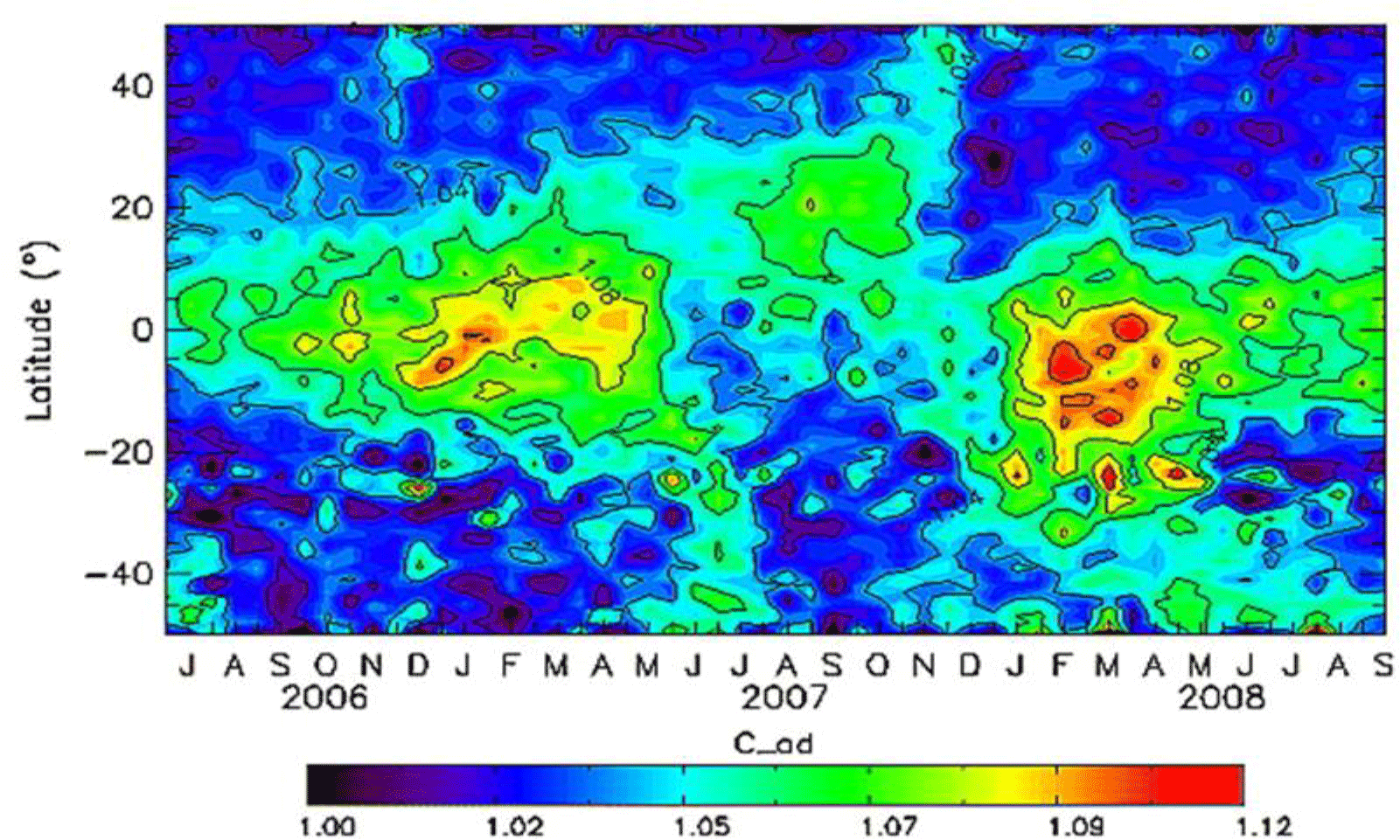
Figure 1Zonally averaged time–latitude cross section of the adjusted calibration coefficient obtained using the CALIOP version 2 data (reproduced from Vernier et al., 2009; copyright 2009 by the American Geophysical Union, with permission from John Wiley and Sons).
As the mission progressed and understanding of data quality improved, it was realized that the calibration altitude could be raised to 36–39 km without compromising the quality of the data products. In order to estimate the scattering ratios expected at the increased CALIOP V4 calibration altitudes, we examined the available stratospheric measurements from other satellites. The most extensive and accurate measurements of stratospheric aerosols have come from the Stratospheric Aerosol and Gas Experiment II (SAGE II) instrument. SAGE II has provided the extinction coefficient profiles in the stratosphere using the solar occultation technique from 1984 through 2005 (Mauldin et al., 1985; Thomason et al., 1997; Damadeo et al., 2013). Between 1991 and 1996, the stratosphere was loaded with volcanic aerosols from the Pinatubo eruption, and no meaningful data are available for that period. Stratospheric aerosol information is also available from the Global Ozone Monitoring by Occultation of Stars (GOMOS) instrument, which provided data up to 2012 (Bertaux et al., 2010; Kyrölä et al., 2010). GOMOS also employs the occultation technique but observes stars rather than the Sun.
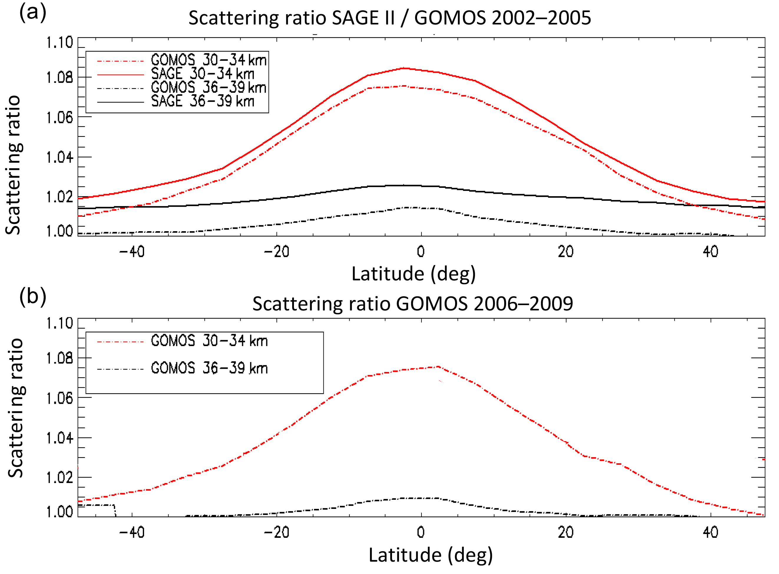
Figure 2Scattering ratio at 30–34 and 36–39 km at 532 nm (a) from SAGE II and GOMOS for the years 2002–2005 and (b) from GOMOS for the years 2006–2009.
Figure 2a shows the zonally averaged scattering ratio (R) at 30–34 km and 36–39 km from both SAGE II (version 7) and GOMOS (version GOPR_6_0) for the time period 2002–2005 at 532 nm. For GOMOS, the aerosol extinctions at 500 nm were converted to R at 532 nm using a stratospheric aerosol lidar ratio of 50 sr and an Ångström exponent of 1.5. A lidar ratio of 50 sr is typically used for quiet non-volcanic (“background”) conditions in the stratosphere (e.g., Kremser et al., 2016), while the value of the Ångström exponent was adopted from the balloon measurements of Jager and Deshler (2002). A similar process was used to convert the SAGE II extinction data at 525 nm to scattering ratios at 532 nm. Both the instruments show significant aerosol scattering ratios of 1.06–1.08 at 30–34 km in the tropics, decreasing to ∼1.02 in the polar regions. On the other hand, at 36–39 km R decreases to ∼1.00–1.02. GOMOS shows a low bias compared to SAGE II in both altitude ranges, with a scattering ratio of ∼1.01 at 36–39 km. Figure 2b shows R in these altitude ranges for 2006–2009 from GOMOS, during the first years of CALIPSO operation. SAGE II data are not available during this period, but as can be seen, the R values at 36–39 km from GOMOS are lower than those during 2002–2005 with a maximum of about 1.01 in the tropics. Assuming SAGE II data to be the reference standard for stratospheric aerosol measurements, and given the uniform underestimate of R from GOMOS as compared to SAGE II (from panel a), it is reasonable to assume a global value of 1.01±0.01 for R at 36–39 km for the period of the CALIPSO mission. This value of R was therefore adopted in the CALIOP V4 algorithm to characterize the aerosol concentration at the new calibration altitude range of 36–39 km.
2.2 CALIOP 532 nm nighttime calibration method
As described in Sects. 2 and 3a of P09, the CALIOP nighttime 532 nm calibration coefficients are derived from the range-corrected, gain- and energy-normalized signals, X(z):
where S(z) is the measured backscatter signal in the 532 nm parallel channel; r is the range, in kilometers, from the lidar to altitude z; E0 is the laser pulse energy continuously measured on the platform; and GA is the electronic amplifier gain adjusted for night and day operation. The calibration coefficients (in km3 sr J−1 count) are derived by normalizing X(z) to the expected backscatter signals computed from an atmospheric scattering model at some calibration altitude zc:
In this equation, R(zc) is the expected scattering ratio that would be measured in the 532 nm parallel channel at the calibration altitude (zc); βm (z) is the molecular backscatter coefficient in the 532 nm parallel channel; and and are the two-way transmittances due to molecular scattering and ozone absorption, given by, respectively,
where σm (z) is the molecular extinction coefficient and is the ozone absorption coefficient.
βm (z), σm (z) and are computed from molecular model data obtained from NASA's GMAO. Accurate calibration of the CALIOP nighttime 532 nm data depends crucially upon this model. Previous versions of the CALIOP data products were generated using the Goddard Earth Observing System Model, Version 5 (GEOS-5) near-real-time analyses, which are created by GMAO for use by NASA satellite instrument teams. These meteorological fields were continually updated with assimilation system improvements and new data inputs. Therefore, successive versions of GMAO data products were used for different time periods during the CALIOP data record. CALIOP versions 3.01 and 3.02 used GEOS 5.2 data. Versions 3.30 and 3.40 used the FP-IT near-real-time assimilation products (GEOS version 5.9.1 and 5.12.4). The initial release of the CALIOP V4 data products (version 4.00) used the FP-IT product built with GEOS 5.9.1. The current V4 release (version 4.10) uses the MERRA-2 reanalysis product (Molod et al., 2015; Gelaro et al., 2017), which has enhanced physics, including a new gravity wave drag parameterization that is capable of producing a quasi- biennial oscillation (QBO), and spans the entire CALIOP data record, from April 2006 to the present. MERRA-2 is thought to provide more accurate modeled meteorological fields because it assimilates temperature and ozone profiles retrieved from the Aura Microwave Limb Sounder (MLS) (Gelaro et al., 2017). Additionally, MERRA-2 also ingests data from new observing systems and has enhanced quality control of conventional sounding data, such as radiosondes (Gelaro et al., 2017). As an example, comparison of CALIOP V3 (created using GEOS-5.2) and V4 (using MERRA-2) data for July 2010 in the calibration region for both V3 and V4, i.e., between 30 and 40 km (including all latitudes), indicates that the fractional difference (V4−V3) / V3 in molecular density varies from zero to about 1.5 %, with a mean difference of ∼0.7 %. The molecular backscatter coefficients between the two models will differ by the same amount. Fractional difference in ozone density (or absorption) varies from about −10 to 5 % with a mean difference of 1.7 %. The resulting total two-way transmittance changes between GEOS-5.2 and MERRA-2 vary from about −0.01 to 0.03 % with a mean difference of ∼0.003 %. These values can vary somewhat with latitude and season. In previous versions of the CALIOP Level 1 data, the aerosol scattering ratio in the 30–34 km calibration region was assumed to be 1; in effect, aerosol loading was assumed to make a negligible contribution to the calculated calibration coefficients. As demonstrated by Vernier et al. (2009), and as anticipated in Hostetler et al. (2006) and P09, this assumption is not valid. In the V4 analyses, the aerosol scattering ratio at altitudes between 36 and 39 km is assumed to be 1.01±0.01, irrespective of latitude.
2.3 The V4 averaging scheme
High-spatial-resolution estimates of the 532 nm nighttime calibration coefficients are generated using profiles that are averaged horizontally over each CALIPSO payload data acquisition cycle (PDAC). A PDAC specifies the minimum time interval over which each of the three CALIPSO instruments can collect an integer number of measurements. During each PDAC, CALIOP acquires backscatter data from 165 laser pulses, which translates into an along-track horizontal distance of ∼55 km. Equation (2) is applied to each vertical range bin within the averaged profile, and from these calculations an estimate of the mean and standard deviation (SD) of the calibration coefficient is determined for each PDAC.
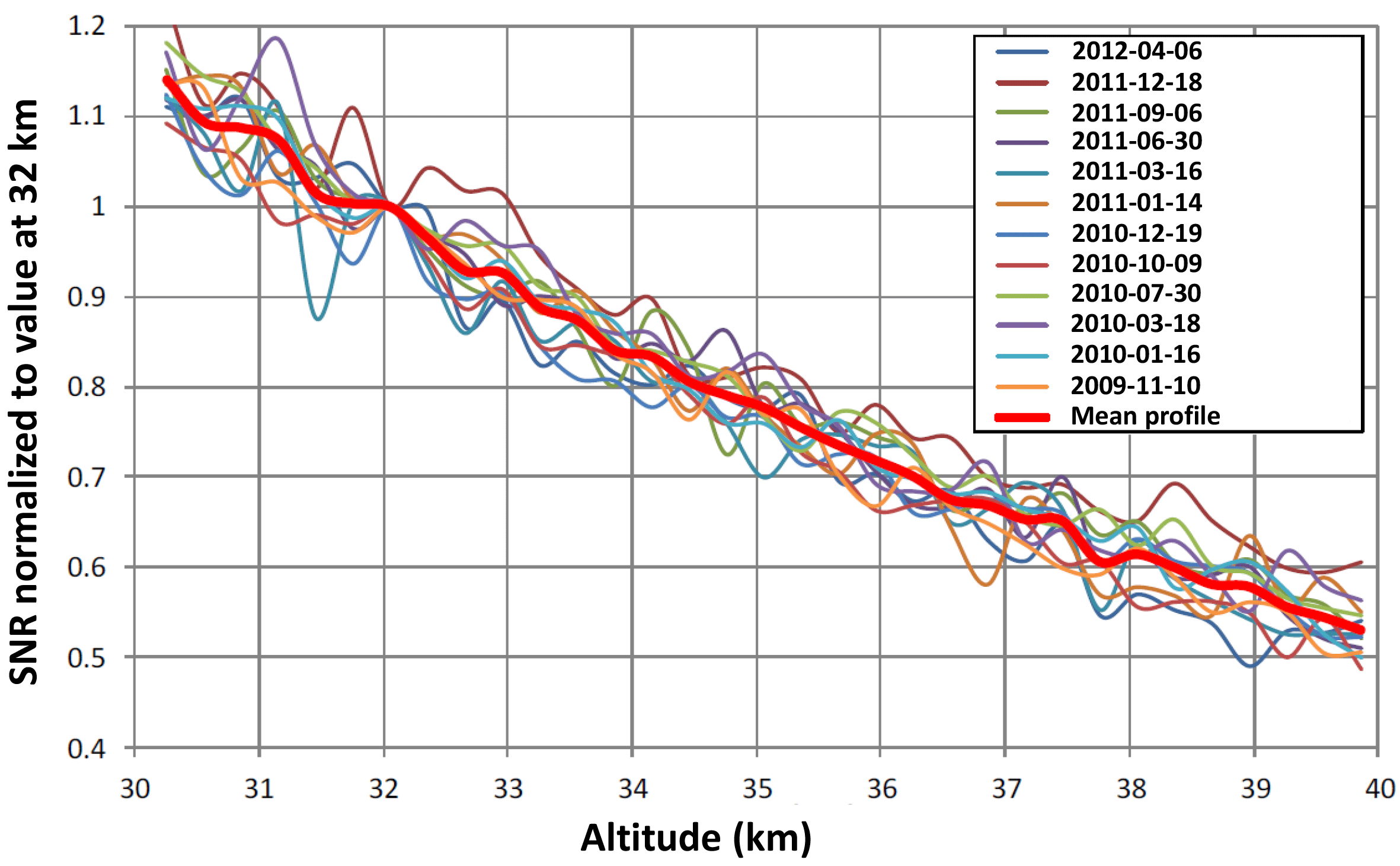
Figure 3Twelve SNR profiles from CALIOP measurements, calculated between 30 km and the maximum CALIOP measurement altitude of 40 km, and representing various latitudes and seasons. The thick red line is the mean profile.
To reduce uncertainties in the final estimates, the calibration coefficients obtained over individual PDACs are further averaged over some fixed spatial extent. In V3 this averaging was done by computing running averages over 27 consecutive PDACs, covering a distance of 1485 km, representing about 8 % of the typical along-track distance for the nighttime segment of the orbit. Calibration coefficients and uncertainty estimates for each laser pulse are then derived by interpolating this time series of smoothed calibration coefficients. Complete mathematical details are given in Sect. 3b of P09.
The quality of the calibration coefficients computed in this manner depends critically on the SNR of the backscattered signal in the calibration region. Based on long-term monitoring of CALIOP's instrument performance, 532 nm parallel channel data measured within the 30–34 km calibration region used in V3 and averaged over 27 consecutive PDACs have an SNR of ∼ 75–80. Figure 3 shows 12 measured profiles of CALIOP SNR as a function of altitude. These profiles are constructed from data acquired from 2009 to 2012, covering all seasons and a wide range of latitudes. The profiles are normalized to have an SNR of 1 at 32 km (i.e., at the mid-point of the V3 calibration region). The relative SNR at 37.5 km (i.e., at the mid-point of the V4 calibration region) is ∼0.65; thus if the averaging procedure used in V3 were to be retained in the V4 calibration region of 36–39 km, the expected SNR of the underlying measurements would drop significantly, to ∼52 (for a SNR of 80 at 32 km). In other words, while raising the calibration region to reduce aerosol contamination provides a substantial decrease in calibration bias errors, random errors can increase by an even larger amount. Because the overall increase in calibration uncertainty introduced by this drop in SNR is unacceptable within the context of the CALIOP Level 2 retrievals (Winker et al., 2009; Young et al., 2013), a new averaging scheme was required for the V4 processing.
Simulations indicate that achieving the V3 SNR at the V4 calibration altitudes within a single orbit would require that the along-track averaging distance be increased to at least 4710 km or 86 PDACs. As this distance represents approximately one quarter of the total along-track distance covered during a nighttime orbit segment, doing this would risk smearing out legitimate time-varying changes in the calibration coefficients. An example of these effects is seen in Fig. 4, which illustrates the thermal beam steering effects that occur near the night-to-day terminator (Hunt et al., 2009). Because these thermally induced calibration variations are highly consistent from orbit to orbit during both daytime and nighttime (Powell et al., 2008), and because longitudinal variations in molecular number density are negligible, an alternative averaging scheme was devised. For V4, high-resolution calibration samples are averaged using a two-dimensional time–space sliding window that extends across-track for 11 consecutive orbits and along-track for 11 consecutive PDACs within each orbit (i.e., 121 PDACs in all, covering a total along-track distance of km). An assessment of multiple years of data verifies that both the instrument and the platform are sufficiently stable to permit averaging over multiple consecutive orbits. The data-averaging procedure runs autonomously during periods of continuous instrument operation. Averaging restarts are initiated for on-orbit instrument tuning events such as boresight alignments and etalon scans, and after any data acquisition interruptions (e.g., due to unfavorable space weather) that extend for more than 24 h. Although more complex to implement than the V3 approach, the V4 averaging strategy has some important advantages, most notably in high-noise regions, where higher-SNR data from adjacent orbits effectively replace the low-SNR samples that would otherwise be used.
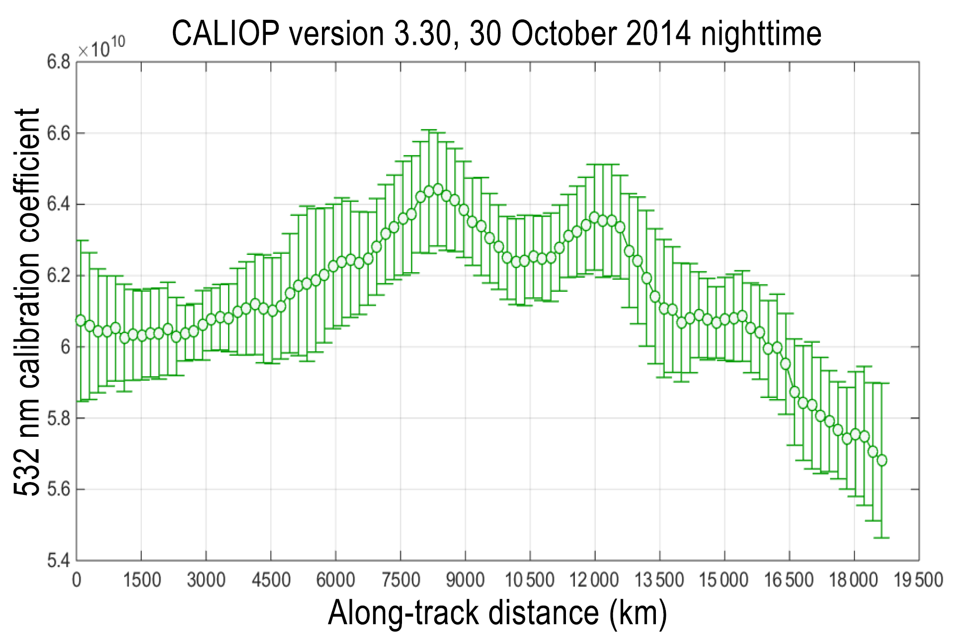
Figure 4Mean 532 nm calibration coefficients (km3 sr J−1 count) in V3 (computed at 30–34 km) as a function of orbit along-track distance computed for all nighttime data acquired on 30 October 2014. The peaks in the curve at ∼8250 km and ∼12 000 km are the result of aerosol contamination in the 30–34 km calibration region. The marked drop-off beginning just after 15 000 km is attributed to thermal beam steering caused by warming as the satellite first enters the sunlit portion of the orbits. For nighttime, the orbit starts in the north, and the starting point of the along-track distance is at the day–night terminator.
2.4 Rejecting outliers in the calibration region
Prior to averaging, the lidar signal profiles are carefully filtered in a three-step process in order to eliminate the large noise spikes that can be encountered in the calibration region. These noise spikes are especially frequent over an extended area covering the continent of South America and adjoining South Atlantic Ocean known as the South Atlantic Anomaly (SAA), where high-energy charged particles from the Sun and cosmic rays trapped in the Van Allen belts come down to relatively low altitudes (Noel et al., 2014; Domingos et al., 2017). Because the CALIOP photomultipliers (PMTs) are not shielded against cosmic radiation, when these charged particles strike the PMT dynode chain they can generate large noise excursions (i.e., “spikes”) that appear at arbitrary altitudes throughout the measured profiles (Hunt et al., 2009). In the first step of the noise rejection process, an adaptive spike filter, outlined in Sect. 3d of P09, is used to remove the outliers from each of the 11 signal profiles (i.e., X(z), averaged to 5 km horizontally and 300 m vertically) measured within a 55 km (165 shot) PDAC. Low and high rejection thresholds are determined based on the expected molecular signal and the uncertainties from the random noise in the measurement process. Further details are given in Sect. 3d of P09. In order to accommodate the generally lower signals at the raised calibration altitudes in the new V4 scheme, the low and high uncertainty threshold values were adjusted so as to eliminate not more than about 0.15 % of the data at both low and high ends of the signal distribution at all latitudes. At least one sample in each range bin in the calibration region for any PDAC is required. Otherwise, the calibration coefficient and its uncertainty for this PDAC are labeled as invalid and excluded from further calibration processing. This is different from V3, where for each failed PDAC, a historical estimate of the calibration coefficient (daily average of all valid calibration coefficients from the previous day) was used (see P09 for details).
As in V3, the valid data in the segments remaining from the first step are further filtered in a second step that removes additional large signal excursions using an estimated noise-to-signal ratio (NSR). The NSR is defined as the SD divided by the mean value of all the valid signals within each PDAC, and the calculated NSR is compared against an empirically derived threshold value. If the NSR value estimated from the valid signal profiles is less than the predefined threshold, then a mean “calibration-ready” profile is constructed from the valid signals. For V4, this step necessitated some careful consideration, particularly at high latitudes in both hemispheres. This is because the molecular number densities (and thus the backscattered signals) drop sharply at high latitudes in local winter. This low signal, coupled with the high incidence of radiation-induced noise (from high-energy particles) at these latitudes, often leads to anomalously high NSR values in the V4 calibration region. Applying the same NSR thresholds that were used in V3 would preferentially eliminate the low-signal/high-noise data at the new calibration altitudes of 36–39 km at these locations and times, leading to high biases in the signal data used for calculating the calibration coefficient, which in turn leads to unrealistically high calibration coefficients in these regions. These high calibration coefficients subsequently yield anomalously low attenuated scattering ratios (<1) in the calibration region and below. In the V3 calibration region, where the SNR was considerably higher, the NSR values are better behaved, and thus the effect is much less pronounced.
Figure 5 shows the NSR thresholds used in V4 as a function of the granule elapsed time (Fig. 5a) and laser footprint latitude (Fig. 5b). Granule elapsed time (in seconds) is referenced to the time at the beginning of a particular orbit segment. For nighttime orbits, the granule elapsed time begins in the northern latitudes at the location of the day-to-night terminator and ends in the southern latitudes where the satellite reaches the night-to-day terminator. The threshold values represent the median NSR plus 5 times the median absolute deviation (MAD) for all Level 1 data acquired during 2007–2012. The NSR thresholds are seen to vary from month to month to accommodate seasonal and latitudinal variations in atmospheric density.
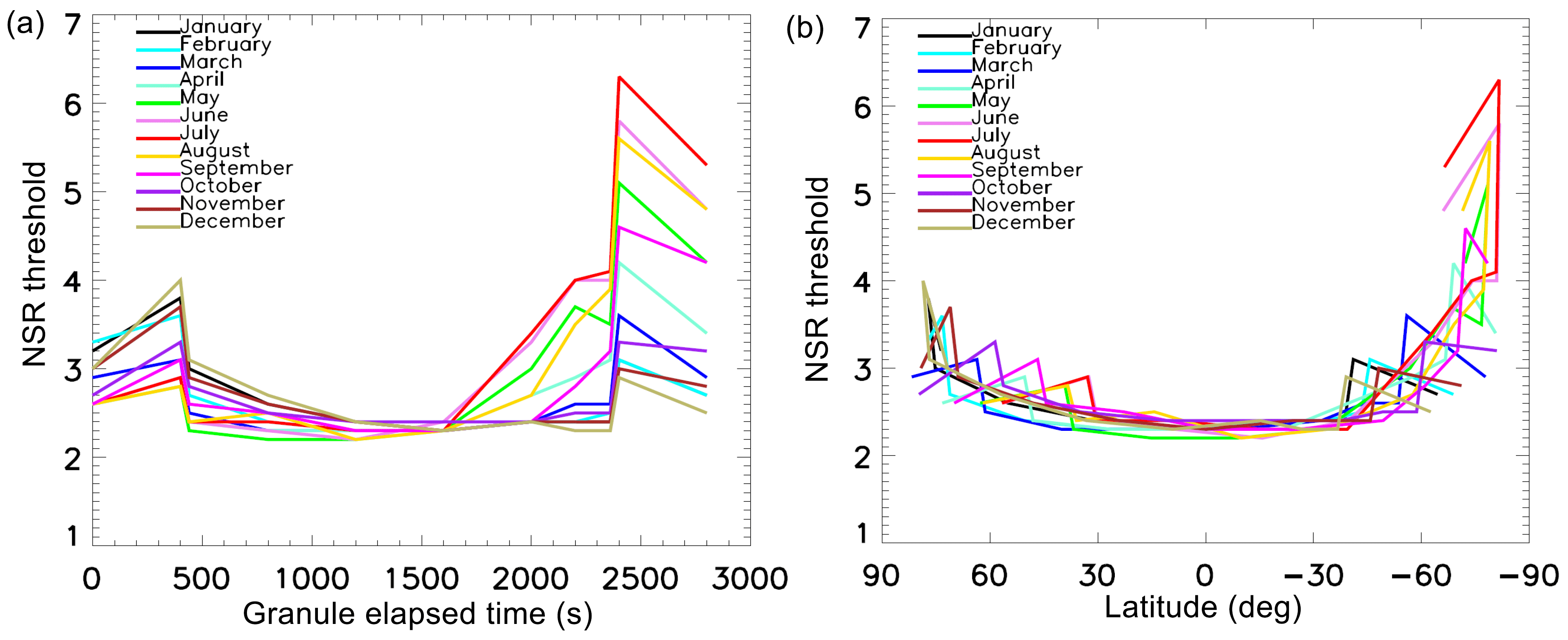
Figure 5The NSR thresholds employed in V4 algorithm for various months (same for all years) as a function of granule elapsed time (a) and latitude (b). The granule elapsed time starts in the Northern Hemisphere at the day-to-night terminator.
The largest seasonal differences occur in the southern polar latitudes, with highest NSR thresholds in local winter, when the densities in the calibration region are lowest. The choice of this particular set of NSR filters was dictated by the requirement that the filter should minimize the difference in mean calibration coefficients over the SAA region and the non-SAA region within the same latitude band. This choice also ensured that at least 85 % of samples (for the test data sets that were used) at all latitudes were retained after filtering for a robust estimation of the calibration coefficient. As mentioned above, the data set used for testing the filters encompassed the years 2007 through 2012, thus including more than 90 % of the data available at that time.

Figure 6Noise-to-signal ratio (blue diamonds) for a single granule (orbit track shown in a) showing the effect of V3 (blue dashed line) and V4 (red line) thresholds. Also plotted are the molecular number densities, averaged over 36–39 km, along the orbit (in magenta). Extreme outliers beyond NSR of 10 and negative values have not been plotted. The granule elapsed time starts at the day-to-night terminator in the Northern Hemisphere.
As an example, Fig. 6b shows the NSR at 36–39 km as a function of the granule elapsed time for a single granule from July 2010. NSR values remain quite uniform at ∼1.5–2.0 until about 1500 s. However, as the molecular number density (averaged over 36–39 km) dips over high southern latitudes, the NSR increases sharply and becomes extremely variable, with large values corresponding to low signal levels. The constant threshold of 3.31 (dashed line in blue) which would have been used by V3 eliminates a substantial fraction of samples at these latitudes. The revised latitudinally variant threshold in V4 (red line) now includes many more of these samples, rejecting only the extreme outliers, and accounts for the high NSR which occurs seasonally at these high latitudes.
In the third and final noise rejection step, an adaptive filter similar to that used in the first step is applied to the mean of the calibration-ready profile. If the mean profile passes this test, then it is used for calculation of the calibration coefficient using Eq. (2). The basic calibration algorithm over a single PDAC with the new spike filter, as mentioned above, is similar in both V3 and V4. Further details with examples of the actual filtering and the mathematical basis for computation of the calibration coefficient are available in P09.
An estimate of the efficiency of the three-step noise rejection algorithm described above may be obtained from the calibration success rate, which is just the ratio of the number of successful calibrations and the attempted calibrations within a specified area.

Figure 7Spatial distribution of the calibration success rates for V3 and V4 for the month of July 2010. The data are binned in in latitude and longitude. Panel (c) shows the difference (V3–V4) in the success rates between the two versions.
Figure 7a and b show the mean single PDAC calibration success rate as a percentage of the calibration opportunities for the month of July 2010 for V3 (Fig. 7a) and V4 (Fig. 7b). Both versions have broadly similar calibration success rates over the globe, with somewhat more noise in V4, as expected due to reduced SNR from the higher calibration region. Over most of the globe, the success rate is over 90 % in both versions. However, substantially lower success rates (in blue) occur over the SAA, where the adaptive filter removes a significant number of PDACs, leading to the lower success rates. The minimum value of the success rate within the SAA region reaches zero. In V3, historical calibration coefficient estimates (daily average from the previous day) were used whenever a PDAC would fail any of the three filtering steps, and these historical values were included in all subsequent averaging operations (see P09 for details). The success rate also falls over Antarctica, with the V4 calibration success rate being somewhat lower than in V3. This phenomenon once again indicates the harsh radiation environment over this area, which affects the SNR particularly at higher altitudes (Hunt et al., 2009). Figure 7c shows the spatial distribution of the difference in success rates between the two versions. Note that there are a few pixels over Antarctica where V3 success rate was higher than V4. This is due to the different and improved noise-filtering scheme in V4. The multi-granule averaging scheme described in Sect. 2.3 is specifically designed to counterbalance the lower single PDAC success rates seen in the V4 data.
2.5 Calculating profiles of attenuated backscatter coefficients
Calculating the calibration coefficients and applying them to the measured profile data is a two-stage process. As described above, the first stage extracts filtered and averaged parallel channel calibration coefficients and uncertainty estimates for each PDAC in all nighttime granules. This procedure uses a two-dimensional sliding window that extends along-track for 11 PDACs and across-track for 11 contiguous nighttime granules. The results obtained from these relatively coarse spatial resolution calibration calculations are stored in a MySQL database. The second calibration stage applies the calibration coefficients to the measured data, resulting in the profiles of calibrated attenuated backscatter coefficients that are reported in the CALIOP L1 data products. For each granule, time histories of the calibration coefficients and their associated uncertainties are retrieved from the database. These data are linearly interpolated with respect to granule elapsed time, tg, for each laser shot along the nighttime orbital track. The interpolated parallel channel calibration coefficients, C|| (tg), are then applied to each parallel channel signal profile, X|| (z, tg), as defined in Eq. (1), to obtain the profile of parallel channel calibrated attenuated backscatter coefficients (in ):
The perpendicular channel signal profiles, , are then calibrated using
where the perpendicular channel calibration coefficient, C⊥ (tg), is the product of C|| (tg) and the polarization gain ratio (PGR) (P09, Eqs. 8–10). The independently calculated PGR quantifies the electronic gain and responsivity differences between the two channels (Hunt et al., 2009). For each laser pulse, the CALIOP L1 data products report the parallel channel calibration coefficient and its corresponding uncertainty. The PGR and its uncertainty are also reported for each laser pulse, and thus the perpendicular channel calibration coefficient and its uncertainty are readily derived. Profiles of the perpendicular channel attenuated backscatter coefficients are also recorded. However, instead of parallel channel attenuated backscatter coefficients, the CALIOP L1 products report the total attenuated backscatter coefficient profiles in per kilometers per steradian, which are simply the sum of the parallel and perpendicular channel contributions. Note that we have explicitly used C|| to denote the parallel channel calibration coefficient in this section to distinguish it from the perpendicular channel calibration coefficient; otherwise C and C|| have been used interchangeably.
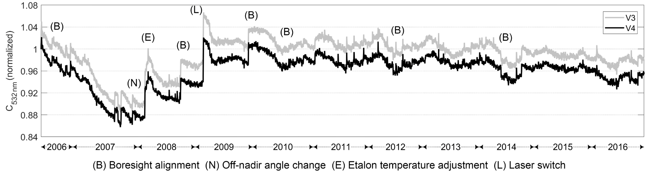
Figure 8Time series of the granule-averaged V3 and V4 532 nm CALIOP nighttime parallel channel calibration coefficient, smoothed over 10 consecutive granules. The values have been normalized by 6.1483×10¹⁰ km3 sr J−1 count. Letters indicate a subset of most significant instrument events that affect the calibration: (B) – boresight alignment; (E) – etalon temperature adjustment; (L) – laser switch; and (N) – off-nadir angle change. Not all events are marked.
Figure 8 shows the time series of the V3 and V4 calibration coefficients from 2006 through 2016. The granule average values of the coefficients have been smoothed over 10 consecutive granules. Overall, there is a decrease of ∼3 % from V3 to V4. Over the short term, sharp upward revisions in calibration mostly correspond to boresight alignment optimizations (marked B in Fig. 8) and etalon temperature tuning procedures, marked E in Fig. 8 (Hunt et al., 2009). These procedures take place periodically and lead to an increase in signal and a corresponding increase in calibration coefficient. Apart from these, there were two significant one-time events that took place. First, the laser off-nadir pointing angle was changed from 0.3 to 3.0∘ in November 2007 (marked N in Fig. 8). Second, CALIPSO's primary laser started showing signs of degradation, and in March 2009 it was replaced by the backup laser, marked L in Fig. 8 (Winker et al., 2010b). The longer-term downward trends in the calibration coefficients are most likely due the slow degradation of receiver components as the instrument ages. The relatively rapid decay in C over the first year of the mission is attributed to a persistently increasing wavelength mismatch between the laser transmitter and the etalon in the receiver (largely corrected by the initial retuning of the etalon in March 2008), compounded by boresight misalignment (Hunt et al., 2009).
3.1 Overall differences between V3 and V4 calibration
Figure 9 shows the spatial distribution of the calibration coefficients for V3 and V4 for the month of October 2010. Several obvious artifacts can be seen in the V3 map. In particular, the band of high values between the Equator and about 50∘ N indicates the calibration biases resulting from aerosol contamination at 30–34 km. Further, the V3 calibration coefficients clearly (and wrongly) demarcate the SAA region, and individual orbital tracks are readily apparent, spuriously suggesting large orbit-to-orbit variations.
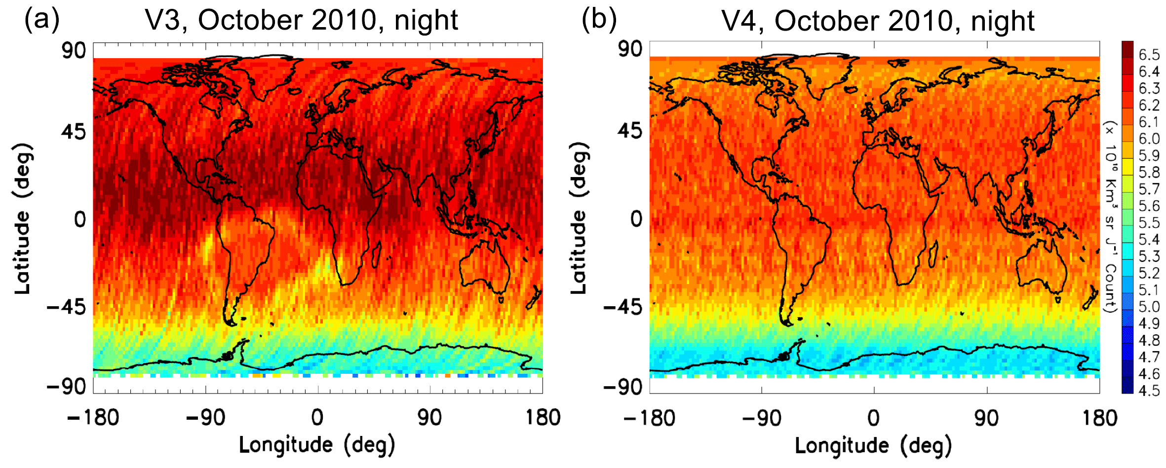
Figure 9Spatial distribution of the 532 nm nighttime calibration coefficient for October 2010, (a) from V3 and (b) from V4.
In contrast, the V4 map is much smoother and shows no indication of any latitudinally varying aerosol contamination. Similarly, the boundaries of the SAA are no longer visible, as the averaging procedure effectively compensates for the low-sampling issues over the noisy regions. The lower values of the calibration coefficient over Antarctica are due to thermal beam steering effects in the instrument that occur as the satellite first enters the sunlit portion of the orbits when approaching the night-to-day terminator (e.g., as seen in Fig. 4).
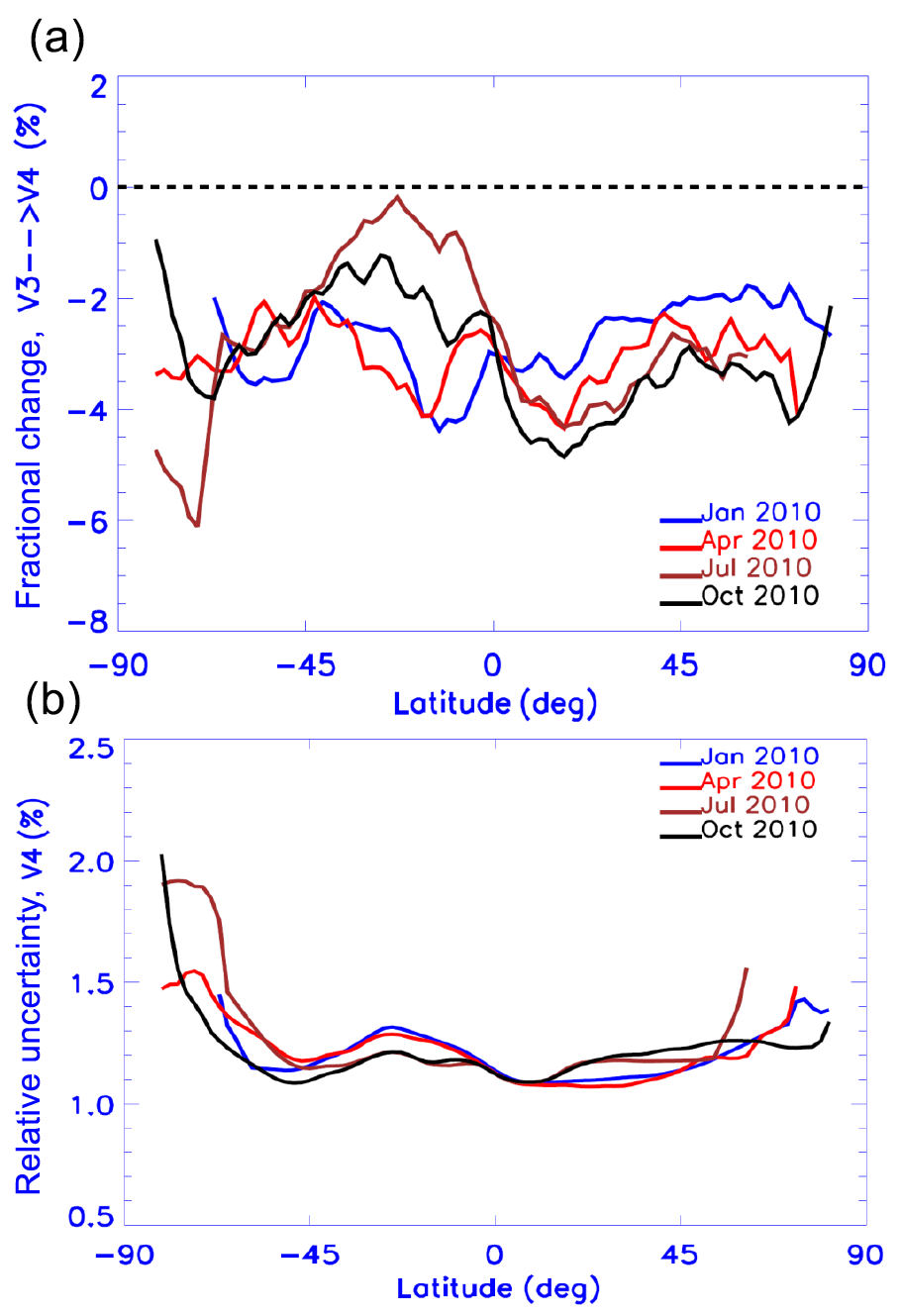
Figure 10The fractional change from V3 to V4, (V4−V3) / V3 in the zonally averaged 532 nm calibration coefficient for 4 months in 2010 (a) and the zonally averaged relative uncertainty (ΔC532 / C532) in the V4 calibration coefficient for the same months (b).
Figure 10a shows the zonal mean distribution of the fractional change in the 532 nm nighttime calibration coefficients from V3 to V4 for the months of January, April, July and October 2010, representing the four seasons. The V4 calibration coefficients, obtained from measurements at 36–39 km, decrease by 2–3 % on average as compared to the V3 calibration coefficients, derived at 30–34 km. This behavior is expected because of the negligibly low aerosol contamination at 36–39 km, as shown in Fig. 2. Seasonal and interannual variations in the calibration differences occur as the aerosol loading at 30–34 km responds to the stratospheric dynamics. One important criterion for improving the calibration in V4 was to retain the same level of the estimated relative random uncertainty in the calibration coefficient. Figure 10b shows the zonal mean relative uncertainty in the calibration coefficient in V4 for the 4 months corresponding to Fig. 10a. Overall, the mean random uncertainty is less than ∼2 %, with higher values over the SAA region and near the poles (particularly in July and October over Antarctica) due to the radiation-induced noise in the measurements in these regions. This is on the same order of uncertainty as in V3. We note, however, that there was a bug in the V3 code that caused the uncertainties reported in the L1 data products to be underestimated by a factor of 3 or more. For this reason, Fig. 10b plots only the V4 uncertainties, not the differences between V3 and V4 that are shown in Fig. 10a.
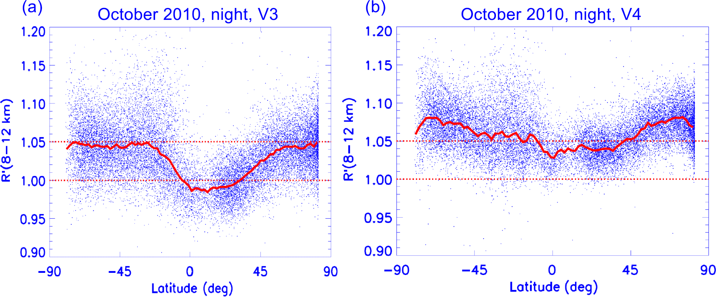
Figure 11Clear-air attenuated scattering ratios at 8–12 km as a function of latitude for the month of October 2010 for V3 (a) and V4 (b). The thick red lines are median values calculated over 2∘ latitude bins.
One of the important signatures indicating suboptimal performance of the V3 532 nm nighttime calibration was a characteristic dip in R′ calculated for “clear-air” conditions in the tropics over an 8–12 km region (P09). R′ values less than unity are not expected under these conditions and essentially imply the existence of aerosols in the V3 calibration region. We note that in this context clear air is not required to be pristine and aerosol-free. Instead, the 8–12 km clear-air samples likely contain tenuous particulate loading at levels that lie below the layer detection threshold of CALIOP but that will still show up as elevated scattering ratios with R′ values in excess of the pristine clear-air R′ of 1.0. Figure 11 shows the clear-air R′ computed between 8 and 12 km for V3 (Fig. 11a) and V4 (Fig. 11b) for October 2010. Each point in this scatterplot represents a 200 km segment along the orbit which has been determined to be clear air (i.e., no cloud or aerosol layers) using the corresponding V3 and V4 Level 2 cloud and aerosol products. The red curves show median values within 2∘ latitude bins. Note that polar stratospheric clouds (PSCs) were additionally cleared for this plot using the currently available version (V1.0) of the CALIOP PSC product (Pitts et al., 2009), which is still based on the CALIOP V3 Level 2 data. As can be seen in Fig. 11, the strong dip in the tropics to median that is seen in V3 data no longer appears in V4, where the median R′ is consistently above ∼1.03. This along with the general meridional uniformity of clear-air R′ indicates a significantly improved calibration in V4 of CALIOP data.
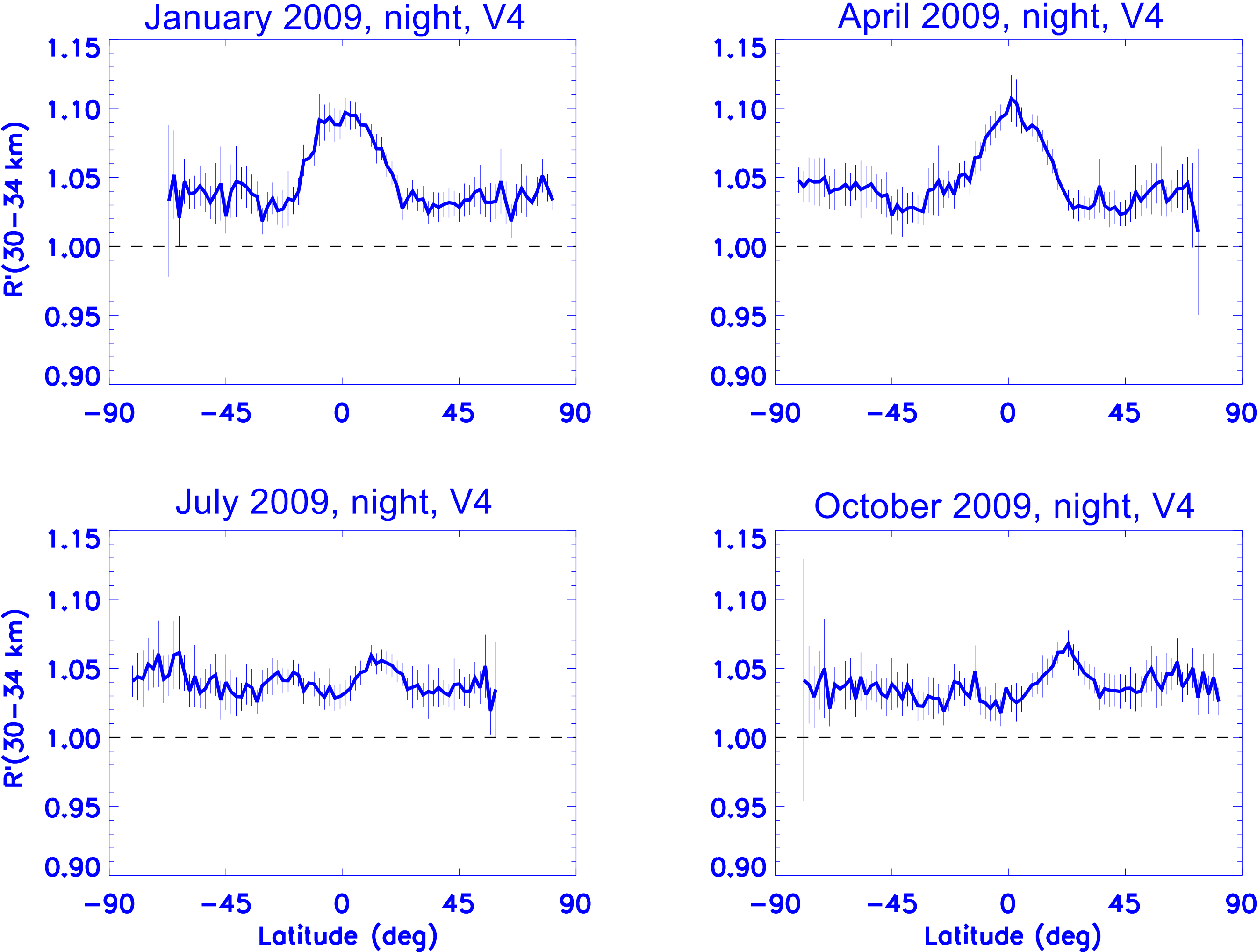
Figure 12Zonally and vertically (over 30–34 km) averaged R′ calculated from V4 CALIOP attenuated backscatter data for January, April, July and October 2009. The data are binned over 2∘ in latitude. The SAA region and bins with fewer than 50 points were not included.
The V3 calibration altitude range of 30–34 km presents a useful region for V4 calibration assessment, since R′ was essentially forced to unity in this region in V3 and should now be different (higher) in V4. Figure 12 shows the zonal mean distribution of R′ averaged over 30–34 km calculated from V4 Level 1 data for January, April, July and October 2009, again representing the four seasons. The R′ values at 30–34 km in V4 represent an increase of between ∼3 to ∼10 % in all cases, with significant seasonal variations. V4 is now consistent with the aerosol loading and its seasonal variation at these altitudes from SAGE II and GOMOS, as seen in Fig. 2, and thus represents a significant improvement over V3. The high tropical values of R′ in January and April, peaking at ∼1.10, may be related to interannual variations in stratospheric dynamics (see Sect. 3.3 below), as was also seen in Fig. 1.
3.2 Effects of instrumental changes on version 4 calibration
As indicated in Fig. 8, several instrument configuration changes have taken place in the CALIOP lidar since the beginning of the mission. Each of these changes results in corresponding changes in the calibration coefficient. A good metric for evaluating the calibration procedure is to ensure that these changes in calibration leave R′ unaffected. In this section we assess this aspect of the V4 calibration.
3.2.1 Laser switch

Figure 13(a) Means and SDs of the zonally averaged 532 nm calibration coefficients normalized by 6.1483×10¹⁰ km3 sr J−1 count, and (b) mean and SD of R′ averaged over 30–34 km. Both time series were calculated using 2 weeks' worth of data before (1–14 February 2009) and after (18–31 March 2009) the laser switch. R′ profiles were calculated over 2∘ latitude intervals from each granule and then averaged over all granules for the latitude bin, with a minimum number of 50 R′ profiles required in each bin. Data over the SAA were not included.
As previously mentioned, the CALIPSO payload includes both a primary laser and a backup laser. At launch, each was housed in a hermetically sealed canister filled with dry air and pressurized to 1 atm (Hunt et al., 2009). CALIOP data production began in June 2006 using the primary laser, which was known pre-launch to have a slow leak in the canister. Over time, as the pressure decreased, the primary laser started showing anomalous behaviors resulting from coronal discharge at low pressures. As a result, the primary laser was turned off on 16 February 2009. The backup laser was subsequently activated on 12 March 2009 and has been continuously operating since then. This is the largest configuration change in the mission so far, and it led to a concomitantly large change in the calibration coefficients. This change is illustrated in Fig. 13, where panel (a) shows the zonal mean calibration coefficients for the 2 weeks immediately before (1–14 February) and immediately after (18–31 March) the laser switch, and panel (b) shows the zonal mean R′ values computed for the same two time periods. While the calibration coefficients are seen to be quite different, the zonal mean R′ values agree quite well. As there were no volcanic eruptions or other meteorological events that perturbed the distribution of stratospheric aerosols during this time period, this close R′ agreement is exactly what should be expected. This clearly demonstrates that the calibration algorithm correctly and automatically adapts to significant changes in instrument configuration without affecting the quality of the science data.
3.2.2 Off-nadir test
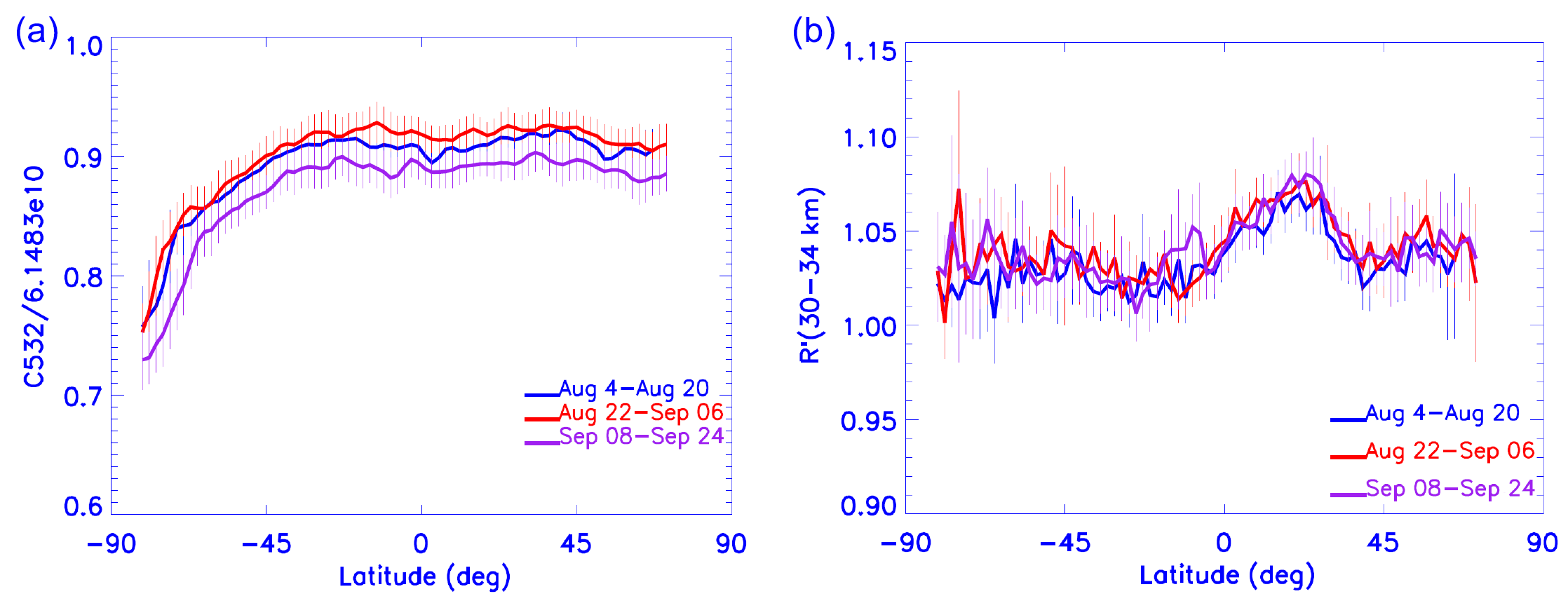
Figure 14As in Fig. 13 but using data before (4–20 August 2007), during (22 August–6 September 2007) and after (8–24 September 2007) the off-nadir laser-pointing test.
Another significant instrument event took place in November 2007, when the pointing angle of the lidar was changed from 0.3 to 3.0∘, in order to minimize the effects of specular reflections from horizontally oriented crystals in ice clouds (Hunt et al., 2009; Noel and Chepfer, 2010). An advanced test of this change was carried out between 22 August and 6 September 2007, when the pointing angle was held at 3∘, and then changed back to 0.3∘ pending the final change in November 2007. Figure 14a shows the normalized calibration coefficients before the test (4–20 August 2007), during the test (22 August–6 September 2007) and after the test (8–24 September 2007). Although not as large as the change resulting from the laser switch, significant changes in the 3∘ off-nadir calibration coefficients can still be discerned among the curves. Note that the calibration coefficients do not exactly revert back to the pre-test values and are somewhat lower. This is because this test took place when the primary laser was still operational and, as seen in Fig. 8, the calibration coefficients were steadily decreasing during this period. However, despite this, the zonal mean R′ values (Fig. 14b) at 30–34 km are all essentially coincident, thus again testifying to the robustness of the calibration algorithm.
3.2.3 Boresight alignment
The alignment between the CALIOP transmitter and receiver is maintained using a boresight mechanism to adjust the laser pointing direction relative to the receiver field of view to maximize the return signal (Hunt et al., 2009). Boresight alignment is checked and adjusted periodically. The boresight alignment that took place on 7 December 2009 resulted in an unusually large adjustment to the previous computed pointing direction. Figure 15a shows zonally averaged calibration coefficients before (21 November–6 December 2009) and after (8–23 December 2009) this boresight alignment. The calibration coefficients changed significantly in response to the event. However, as can be seen in Fig. 15b, changes in stratospheric R′ are largely negligible and are not correlated with the changes in the calibration coefficients. At a couple of locations, the R′ curves show significant deviations, which could be due to some real variations in aerosol loading or noise in the data.
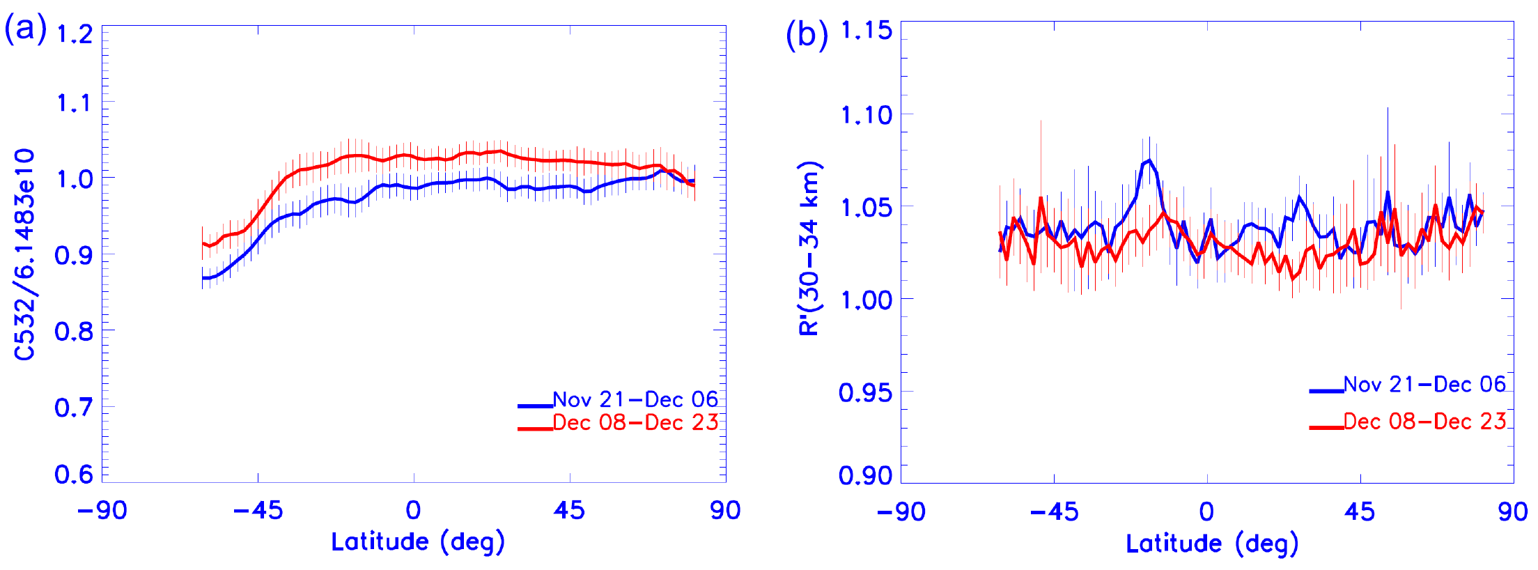
Figure 15Same as in Fig. 13 but using data before (21 November–6 December 2009) and after (8–23 December 2009) the boresight alignment procedure on 7 December 2009.
3.3 Representation of stratospheric aerosol
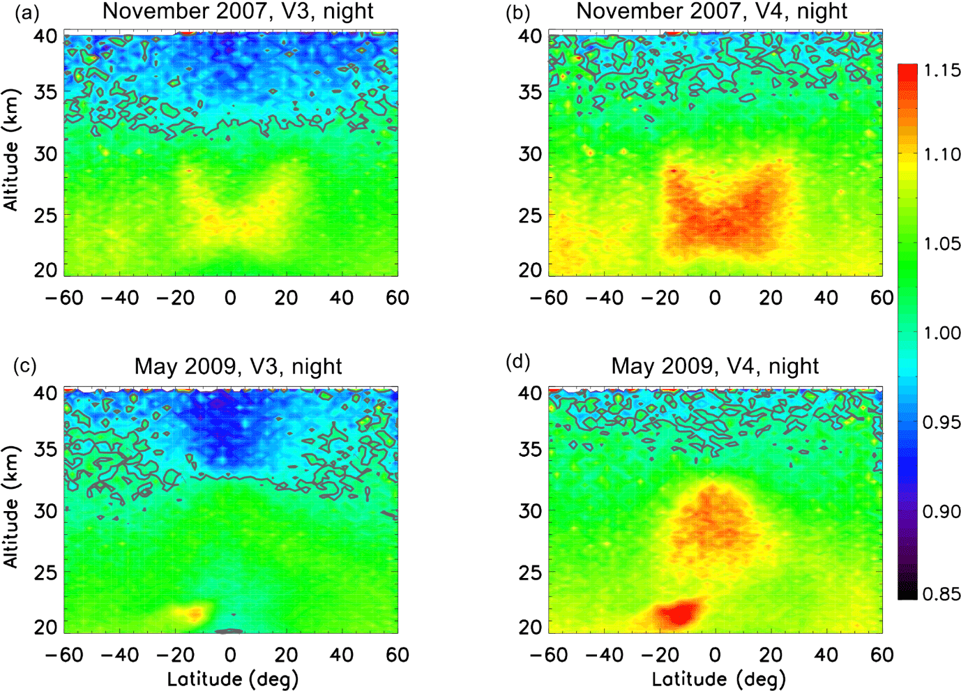
Figure 16Zonally averaged height–latitude cross sections of R′ calculated using V3 and V4 Level 1 data for November 2007 (a, b) and for May 2009 (c, d). The contour lines shown are for .
As demonstrated above, the new calibration coefficients in V4 lead to a generally upward revision of the Level 1 attenuated backscatter coefficients by 3–6 % or more, depending upon location and season. In particular, Fig. 12 indicates that variations in aerosol loading at stratospheric altitudes are robustly captured in the V4 data. This is illustrated further in Fig. 16, which shows the zonally averaged height–latitude cross sections of R′ in November 2007 and May 2009 for both V3 and V4. In both months, distinct structures can be observed in the V4 data in the stratospheric regions between 20 and 30 km in the tropics which are likely linked to the QBO of lower stratospheric winds between about 20 and 35 km. In November 2007, a dominant westerly shear prevailed in the stratosphere (monthly mean zonal wind at Singapore at 10 hPa =18 ms−1), leading to a characteristic double-horn structure in the tropical stratospheric aerosol distribution (Trepte and Hitchman, 1992). In the V3 map (Fig. 16a) this structure can be seen only partially, while it is much more prominent and clear in the V4 map (Fig. 16b). On the other hand, a dominant easterly shear prevailed in the stratosphere in May 2009 (monthly mean zonal wind at Singapore at 34.2 ms−1), during which aerosol lofting is expected to take place in the tropics and lateral transport is inhibited (Trepte and Hitchman, 1992). The aerosol lofting is not seen in the V3 map (Fig. 16c) but is quite clearly observed in the V4 map (Fig. 16d). This illustrates the potential for V4 CALIOP data to provide important and robust information on stratospheric aerosol. A CALIOP stratospheric aerosol product is currently under development which exploits the improved V4 calibration.
The airborne HSRL developed at NASA LaRC (Hair et al., 2008) has been used throughout the CALIPSO mission to validate the CALIOP lidar calibration through an ongoing series of coincident underflights (Rogers et al., 2011). At 532 nm, the HSRL uses an internal calibration technique that avoids the aerosol contamination issues at calibration altitudes encountered by spaceborne lidars and thus can deliver highly accurate measurements (to within ∼1 %) of attenuated backscatter coefficients (Rogers et al., 2011). Following the procedures outlined in Rogers et al. (2011), a total of 35 nighttime flights conducted between June 2006 and June 2014 were used for comparison with the coincident CALIOP measurements in clear-air conditions. For comparison with CALIOP, the total attenuated backscatter measured by the HSRL must first be corrected for the molecular and ozone attenuation between the HSRL flight altitude (typically ∼8–9 km above mean sea level) and the CALIOP altitude. These corrections are made using the same atmospheric model data used in deriving the CALIOP calibration coefficients. Following the protocol described in Rogers et al. (2011), the V4 CALIOP vertical feature mask (VFM) is used to exclude all profiles in which layers are detected above the HSRL aircraft altitude. Upon completion of this procedure, averaged attenuated backscatter profiles are created for both sets of measurements. The amount of horizontal averaging performed for the comparisons varies from flight to flight, and it depends upon the temporal–spatial collocation of the CALIPSO and the HSRL data sets. The vertical extent of the regions used in the comparisons also varies, depending on the geometric depth of the clear-air segments within the averaged profiles. Fractional difference profiles between HSRL and CALIOP are then calculated using
where is the mean of the coincident total attenuated backscatter from the HSRL at range r, referenced to the CALIOP altitude grid, and is the corresponding mean of total attenuated backscatter from CALIOP at range r. For further details of the comparison methodology, the reader is referred to Rogers et al. (2011). A single difference value was estimated for each HSRL coincident underflight by averaging over the horizontal and vertical dimensions of the clear-air region. Figure 17 shows the mean biases between HSRL and CALIOP using all clear-air data from each individual underflight as a function of mean latitude for both the V3 (filled diamonds) and V4 (open circles) data sets.
Most of the flights took place at the northern midlatitudes between 30–40∘ N (Fig. 17). Although the comparison covers only a limited latitude range, no obvious latitude dependence can be discerned. In general, the low bias of the CALIOP attenuated backscatter coefficients was more pronounced in V3 and has now decreased in V4, which shows a more uniform distribution of points about the zero difference line. Most of the differences from the individual flights have decreased significantly, with the exception of a few outliers. Rogers et al. (2011) pointed out a slight seasonal effect in the V3 biases with somewhat higher bias during the summer months, which might be related to enhanced stratospheric aerosol loading. The improved calibration in V4 has now generally reduced the differences during the summer months. The mean bias between the two instruments for V4 calibration using data from all the flights is 1.6 %±2.4 % and has decreased from 3.6 %±2.2 % in V3. When computing these aggregate means and SDs, the sample counts from each flight are used as weights that are applied to the per-flight means and SDs.
Note that we expect the CALIOP attenuated backscatter coefficients to be slightly lower than those from HSRL, as we cannot correct the HSRL data for the attenuation from undetected aerosols (or clouds) that occurs between the CALIPSO satellite and the HSRL aircraft altitudes. The stratospheric aerosol optical depth (SAOD) at 525 nm in the tropics (20∘ S–20∘ N) between the tropopause and 40 km has been declining steadily in the post-Pinatubo period, reaching very low values of ∼0.003 in 2001–2002 (Kremser et al., 2016). Subsequently SAOD rose slowly because of inputs from moderate-size volcanic eruptions leading to a value of about 0.005 on average between 2006 and 2012 (Vernier et al., 2011; Kremser et al., 2016). Assuming then a background SAOD of 0.005 at 532 nm, the failure to correct for this attenuation would account for about 1 % of the 1.6 % mean bias estimated using V4 CALIOP data.
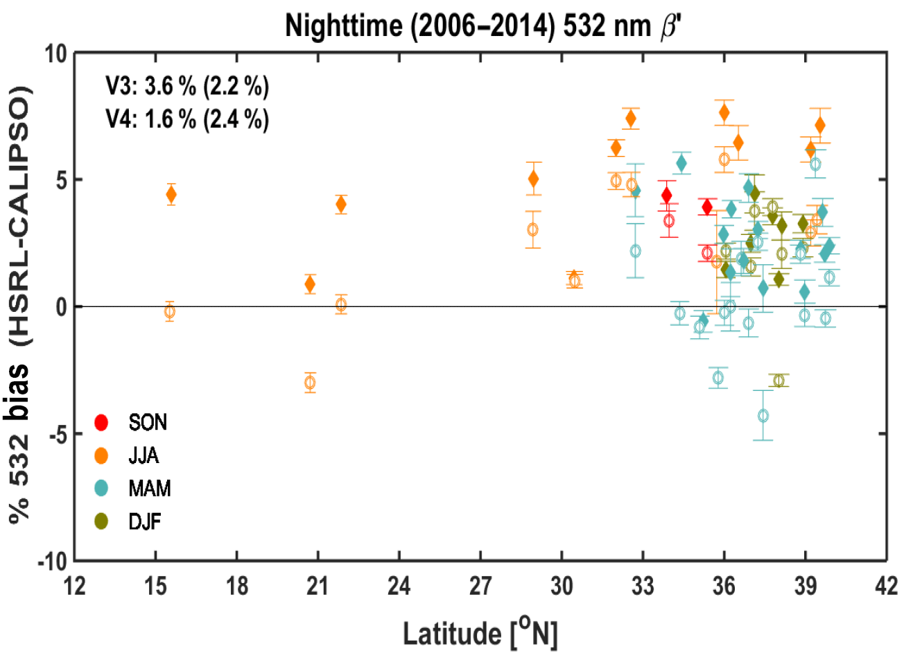
Figure 17Difference between HSRL and CALIOP attenuated backscatter measurements for nighttime clear-air profiles as a function of latitude. The data are colored by the season of measurement. V3 differences are shown as filled diamonds, and the corresponding V4 differences are shown as open circles. The error bars for each point represent the SD of the mean.
We note too that the V3 values reported here differ slightly from those given in Rogers et al. (2011). There are two reasons for this. First, the number of HSRL flights available for comparison has increased since 2011, and hence the sample size in the new study is somewhat larger. Second, and perhaps more important, a bug discovered in the analysis code used for the original study led to slight underestimates of the bias calculations. Further details of this bug and its remediation are given in Appendix A.
The 532 nm nighttime calibration is the fundamental quantity from which all other CALIOP calibration coefficients are derived, and thus it is the most important element in ensuring the robustness and overall quality of the CALIOP data products. The V4 algorithm incorporates two major changes that markedly improve the accuracy and reliability of the 532 nm nighttime calibration. First, the calibration altitude range for the nighttime parallel channel has been raised from 30–34 to 36–39 km, resulting in significantly reduced contamination from stratospheric aerosols (now at about the 1 % level) for the molecular normalization procedure. And second, a new two-dimensional averaging scheme that harvests data both along an orbit track and across multiple adjacent orbit tracks ensures that the random error in the calibration coefficients is at or below the levels reported in the V3 data products. Among other important changes are an improved noise-filtering scheme, the adoption of MERRA-2 as the meteorological model and the explicit accounting for the presence of residual aerosol in the calibration region. We have presented the salient features of the new calibration procedure and highlighted the many improvements in the V4 data arising from this new calibration. The inconsistencies in the V3 data owing to the previous calibration scheme have largely been resolved. The relative uncertainties from random noise in the V4 calibration are of the same magnitude as they were in V3, and the V4 calibration procedure is shown to correctly adjust to compensate for periodic instrument changes such as boresight alignments. The new calibration also improves the representation of stratospheric aerosols that will be exploited in future versions of the CALIOP data products. Importantly, validation of the V4 nighttime calibration coefficients using the coincident HSRL measurements at northern midlatitudes indicates an agreement to within %, reduced from 3.6 %±2.2 % in V3, indicating a robust enhancement in calibration accuracy. Overall, a significant improvement in CALIOP primary calibration has been achieved in V4 which will result in corresponding improvements in the downstream Level 1 and Level 2 CALIOP products. In particular, the attenuated backscatter values increase by about 2–3 % on average, which enables increased detection of tenuous layers by the Level 2 algorithm, particularly in the stratosphere. The improvements in stratospheric aerosol retrievals will be invaluable for cross-validation of the stratospheric aerosol products from other instruments, such as the Stratospheric Aerosol and Gas Experiment III on International Space Station (SAGE III-ISS), and are expected to lead to a better understanding of climate-related issues.
CALIPSO lidar Level 1b data products are publicly available at the Atmospheric Science Data Center at NASA LaRC (https://eosweb.larc.nasa.gov/project/calipso/calipso_table; National Aeronautics and Space Administration, 2018a) and at the AERIS/ICARE Data and Services Center (http://www.icare.univ-lille1.fr). The SAGE II data products are also publicly available at the Atmospheric Science Data Center (https://eosweb.larc.nasa.gov/project/sage2/sage2_table; National Aeronautics and Space Administration, 2018b). HSRL data are available by request from the authors (Mark Vaughan at mark.a.vaughan@nasa.gov) or from the NASA-Langley HSRL team (John Hair at johnathan.w.hair@nasa.gov).
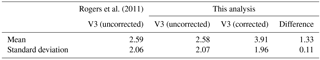
When replicating the analyses of the collocated CALIOP–HSRL data set for this paper, an error was discovered in the code used to estimate the overlying two-way transmittance differences between the two sets of measurements. This error led to a small bias in the results reported in Rogers et al. (2011). We thus report here updated values for the V3 data set calculated using the corrected code. Table A1 shows the mean and the SD of the mean computed from a data set of column-averaged biases for each HSRL flight. Note that the uncorrected V3 values do not exactly match those of Rogers et al. (2011) due to slight variations in the code and flight data used. A difference of ∼1.3 % (corrected−uncorrected) in the mean bias is found, which represents an underestimation of the bias reported previously. However, the results shown in this study still show a significant improvement in the calibration scheme for the V4 CALIOP data.
Table A1The HSRL–CALIOP biases as calculated by Rogers et al. (2011) and after correction of a coding error.
Authors Charles R. Trepte and Jacques Pelon are co-guest-editors for the “CALIPSO version 4 algorithms and data products” special issue in Atmospheric Measurement Techniques but did not participate in any aspects of the editorial review of this paper. All other authors declare that they have no conflicts of interest.
This article is part of the special issue “CALIPSO version 4 algorithms and data products”. It is not affiliated with a conference.
We are grateful to Laurent Blanot and the GOMOS team for providing
us with the GOMOS data. Figure 1 was reproduced (copyright 2009
American Geophysical Union) with permission from John Wiley and
Sons. This paper is dedicated to the memory of William H. Hunt. The
referees are thanked for useful comments which helped improve the
quality of the paper.
Edited by: Vassilis Amiridis
Reviewed by: Franco Marenco and two anonymous referees
Behrenfeld, M. J., Hu, Y., O'Malley, R. T., Boss, E. S., Hostetler, C. A., Siegel, D. A., Sarmiento, J. L., Schulien, J., Hair, J. W., Lu, X., Rodier, S., and Scarino, A. J.: Annual boom – bust cycles of polar phytoplankton biomass revealed by space-based lidar, Nat. Geosci., 10, 118–122, https://doi.org/10.1038/ngeo2861, 2017.
Bertaux, J. L., Kyrölä, E., Fussen, D., Hauchecorne, A., Dalaudier, F., Sofieva, V., Tamminen, J., Vanhellemont, F., Fanton d'Andon, O., Barrot, G., Mangin, A., Blanot, L., Lebrun, J. C., Pérot, K., Fehr, T., Saavedra, L., Leppelmeier, G. W., and Fraisse, R.: Global ozone monitoring by occultation of stars: an overview of GOMOS measurements on ENVISAT, Atmos. Chem. Phys., 10, 12091–12148, https://doi.org/10.5194/acp-10-12091-2010, 2010.
Damadeo, R. P., Zawodny, J. M., Thomason, L. W., and Iyer, N.: SAGE version 7.0 algorithm: application to SAGE II, Atmos. Meas. Tech., 6, 3539–3561, https://doi.org/10.5194/amt-6-3539-2013, 2013.
Domingos, J., Jault, D., Pais, M. A., and Mandea, M.: The South Atlantic Anomaly throughout the solar cycle, Earth Planet. Sc. Lett., 473, 154–163, https://doi.org/10.1016/j.epsl.2017.06.004, 2017.
Garnier, A., Scott, N. A., Pelon, J., Armante, R., Crépeau, L., Six, B., and Pascal, N.: Long-term assessment of the CALIPSO Imaging Infrared Radiometer (IIR) calibration and stability through simulated and observed comparisons with MODIS/Aqua and SEVIRI/Meteosat, Atmos. Meas. Tech., 10, 1403–1424, https://doi.org/10.5194/amt-10-1403-2017, 2017.
Gelaro, R., McCarty, W., Suarez, M. J., Todling, R., Molod, A., Takacs, L., Randles, C. A., Darmenov, A., Bosilovich, M. G., Reichle, R., Wargan, K., Coy, L., Cullather, R., Draper, C., Akella, S., Buchard, V., Conaty, A., Da Silva, A. M., Gu, W., Kim, G.-K., Koster, R., Lucchesi, R., Markova, D., Nielsen, J. E., Partyka, G., Pawson, S., Putman, W., Rienecker, M., Schubert, S. C., Sienkiewicz, M., and Zhao, B.: The Modern-Era Retrospective Analysis for Research and Applications, Version 2 (MERRA-2), J. Climate, 30, 5419–5454, https://doi.org/10.1175/JCLI-D-16-0758.1, 2017.
Getzewich, B., Vaughan, M., Hunt, W., Avery, M., Tackett, J., Kar, J., and Lee, K.-P.: CALIPSO Lidar Calibration at 532 nm: Version 4 Daytime Algorithm, in preparation, 2018.
Gimmestad, G., Forrister, H., Grigas, T., and O'Dowd, C., Comparisons of aerosol backscatter using satellite and ground lidars: Implications for calibrating and validating space borne lidar, Sci. Rep.-UK, 7, 42337, https://doi.org/10.1038/srep42337, 2017.
Hair, J. W., Hostetler, C. A., Cook, A. L., Harper, D. B., Ferrare, R. A., Mack, T. L., Welch, W., Isquierdo, L. R., and Hovis, F. E.: Airborne High Spectral Resolution Lidar for profiling aerosol optical properties, Appl. Optics, 47, 6734–6752, https://doi.org/10.1364/AO.47.006734, 2008.
Hostetler, C. A., Liu, Z., Reagan, J., Vaughan, M., Winker, D., Osborn, M., Hunt, W. H., Powell, K. A., and Trepte, C.: CALIOP Algorithm Theoretical Basis Document, Calibration and Level 1 Data Products, PC-SCI-201, NASA Langley Research Center, Hampton, VA 23681, 66 pp., available at: http://www-calipso.larc.nasa.gov/resources/project_documentation.php (last access: 12 March 2018), 2006.
Hu, Y., Winker, D., Vaughan, M., Lin, B., Omar, A., Trepte, C., Flittner, D., Yang, P., Sun, W., Liu, Z., Wang, Z., Young, S., Stamnes, K., Huang, J., Kuehn, R., Baum, B., and Holz, R.: CALIPSO/CALIOP Cloud Phase Discrimination Algorithm, J. Atmos. Ocean. Tech., 26, 2293–2309, https://doi.org/10.1175/2009JTECHA1280.1, 2009.
Hunt, W. H., Winker, D. M., Vaughan, M. A., Powell, K. A., Lucker, P. L., and Weimer, C.: CALIPSO Lidar description and performance assessment, J. Atmos. Ocean. Tech., 26, 1214–1228, https://doi.org/10.1175/2009JTECHA1223.1, 2009.
Jager, H. and Deshler, T.: Lidar backscatter to extinction, mass and area conversions for stratospheric aerosols based on midlatitude balloonborne size distribution measurements, Geophys. Res. Lett., 29, 1929, https://doi.org/10.1029/2002GL015609, 2002.
Kremser, S., Thomason, L. W., von Hobe, M., Hermann, M., Deshler, T., Timmreck, C., Toohey, M., Stenke, A., Schwarz, J. P., Weigel, R., Fueglistaler, S., Prata, F. J., Vernier, J.-P., Schlager, H., Barnes, J. E., Antuna-Marrero, J.-C., Fairlie, D., Palm, M., Mahieu, E., Notholt, J., Rex, M., Bingen, C., Vanhellemont, F., Bourassa, A., Plane, J. M. C., Kolcke, D., Carn, S. A., Clarisse, L., Trickl, T., Neely, R., James, A. D., Rieger, L., Wilson, J. C., and Meland, B.: Stratospheric aerosol-Observations, processes and impact on climate, Rev. Geophys., 54, 278–335, https://doi.org/10.1002/2015RG000511, 2016.
Kyrölä, E., Tamminen, J., Sofieva, V., Bertaux, J. L., Hauchecorne, A., Dalaudier, F., Fussen, D., Vanhellemont, F., Fanton d'Andon, O., Barrot, G., Guirlet, M., Mangin, A., Blanot, L., Fehr, T., Saavedra de Miguel, L., and Fraisse, R.: Retrieval of atmospheric parameters from GOMOS data, Atmos. Chem. Phys., 10, 11881–11903, https://doi.org/10.5194/acp-10-11881-2010, 2010.
Liu, Z. Vaughan, M., Winker, D., Kittaka, C., Getzewich, B., Kuehn, R., Omar, A., Powell, K., Trepte, C., and Hostetler, C.: The CALIPSO lidar cloud and aerosol discrimination: Version 2 Algorithm and initial assessment of performance, J. Atmos. Ocean. Tech., 26, 1198–1212, 2009.
Mamouri, R. E., Amiridis, V., Papayannis, A., Giannakaki, E., Tsaknakis, G., and Balis, D. S.: Validation of CALIPSO space-borne-derived attenuated backscatter coefficient profiles using a ground-based lidar in Athens, Greece, Atmos. Meas. Tech., 2, 513–522, https://doi.org/10.5194/amt-2-513-2009, 2009.
Mauldin III, L. E., Zaun, N, H., McCormick, M. P., Guy, J. H., and Vaughan, W. R.: Stratospheric aerosol and gas experiment II instrument: A functional description, Opt. Eng., 24, 307–312, 1985.
Molod, A., Takacs, L., Suarez, M., and Bacmeister, J.: Development of the GEOS-5 atmospheric general circulation model: evolution from MERRA to MERRA2, Geosci. Model Dev., 8, 1339–1356, https://doi.org/10.5194/gmd-8-1339-2015, 2015.
Mona, L., Pappalardo, G., Amodeo, A., D'Amico, G., Madonna, F., Boselli, A., Giunta, A., Russo, F., and Cuomo, V.: One year of CNR-IMAA multi-wavelength Raman lidar measurements in coincidence with CALIPSO overpasses: Level 1 products comparison, Atmos. Chem. Phys., 9, 7213–7228, https://doi.org/10.5194/acp-9-7213-2009, 2009.
National Aeronautics and Space Administration: CALIPSO data and information, available at: https://eosweb.larc.nasa.gov/project/calipso/calipso_table, last access: 12 March 2018a.
National Aeronautics and Space Administration: SAGE II data and information, available at: https://eosweb.larc.nasa.gov/project/sage2/sage2_table, last access: 12 March 2018b.
Omar, A., Winker, D. M., Kittaka, C., Vaughan, M., Liu, Z., Hu, Y., Trepte, C. R., Rogers, R. R., Ferrare, R. A., Lee, K-P, Kuehn, R. E., and Hosteler, C. A.: The CALIPSO automated aerosol classification and lidar ratio selection algorithm, J. Atmos. Ocean. Tech., 26, 1994–2014, 2009.
Noel, V. and Chepfer, H.: A global view of horizontally-oriented crystals in ice clouds from CALIPSO, J. Geophys. Res., 115, D00H23, https://doi.org/10.1029/2009JD012365, 2010.
Noel, V., Chepfer, H., Hoareau, C., Reverdy, M., and Cesana, G.: Effects of solar activity on noise in CALIOP profiles above the South Atlantic Anomaly, Atmos. Meas. Tech., 7, 1597–1603, https://doi.org/10.5194/amt-7-1597-2014, 2014.
Pappalardo, G., Wandinger, U., Mona, L., Hiebsch, A., Mattis, I., Amodeo, A., Ansmann, A., Seifert, P., Linne, H., Apituley, A., Alados Arboledas, L., Balis, D., Chaikovsky, A., D'Amico, G., De Tomasi, F., Freudenthaler, V., Giannakaki, E., Giunta, A., Grigorov, I., Iarlori, M., Madonna, F., Mamouri, R.-E., Nasti, L., Papayannis, A., Pietruczuk, A., Pujadas, M., Rizi, V., Rocadenbosch, F., Russo, F., Schnell, F., Spinelli, N., Wang, X., and Wiegner, M.: EARLINET correlative measurements for CALIPSO: first intercomparison results, J. Geophys. Res., 115, D00H19, https://doi.org/10.1029/2009JD012147, 2010.
Pitts, M. C., Poole, L. R., and Thomason, L. W.: CALIPSO polar stratospheric cloud observations: second-generation detection algorithm and composition discrimination, Atmos. Chem. Phys., 9, 7577–7589, https://doi.org/10.5194/acp-9-7577-2009, 2009.
Powell, K. A., Vaughan, M. A., Kuehn, R., Hunt, W. H., and Lee, K.-P.: Revised Calibration Strategy for the CALIOP 532-nm Channel: Part II – Daytime, in: Reviewed and Revised Papers Presented at the 24th International Laser Radar Conference, 23–27 June, 2008, Boulder, CO, USA, 1177–1180, 2008.
Powell, K. A., Hostetler, C. A., Liu, Z., Vaughan, M. A., Kuehn, R. A., Hunt, W. H., Lee, K.-P. Trepte, C. R., Rogers, R. R., Young, S. A., and Winker, D. M.: CALIPSO Lidar calibration algorithms. Part I: Nighttime 532 nm parallel channel and 532 nm perpendicular channel, J. Atmos. Ocean. Tech., 26, 2015–2033, https://doi.org/10.1175/2009JTECHA1242.1, 2009.
Rogers, R. R., Hostetler, C. A., Hair, J. W., Ferrare, R. A., Liu, Z., Obland, M. D., Harper, D. B., Cook, A. L., Powell, K. A., Vaughan, M. A., and Winker, D. M.: Assessment of the CALIPSO Lidar 532 nm attenuated backscatter calibration using the NASA LaRC airborne High Spectral Resolution Lidar, Atmos. Chem. Phys., 11, 1295–1311, https://doi.org/10.5194/acp-11-1295-2011, 2011.
Russell, P. B., Swissler, T. J., and McCormick, M. P.: Methodology for error analysis and simulation of lidar aerosol measurements, Appl. Optics, 18, 3783–3797, https://doi.org/10.1364/AO.18.003783, 1979.
Santer, B. D., Solomon, S., Bonfils, C., Zelinka, M. D., Painter, J. F., Beltran, F., Fyfe, J. C., Johannesson, G., Mears, C., Ridley, D. A., Vernier, J.-P., and Wentz, F. J.: Observed multi-variable signals of late 20th and early 21st century volcanic activity, Geophys. Res. Lett., 42, 500–509, https://doi.org/10.1002/2014GL062366, 2015.
Solomon, S., Daniel, J. S., Neely III, R. R., Vernier, J.-P., Dutton, E. G., and Thomason, L. W.: The persistently variable “Background” stratospheric aerosol layer and global climate change, Science, 333, 866–870, https://doi.org/10.1126/science.1206027, 2011.
Tan, I., Storelvmo, T., and Zelinka, M. D.: Observational constraints on mixed-phased cloud simply higher climate sensitivity, Science, 352, 224–227, https://doi.org/10.1126/science.aad5300, 2016.
Thomason, L. W., Poole, L. R., and Deshler, T. R.: A global climatology of stratospheric aerosol surface area density as deduced from SAGE II: 1984, 1994, J. Geophys. Res., 102, 8967–8976, 1997.
Trepte, C. R. and Hitchman, M. H.: Tropical stratospheric circulation deduced from satellite aerosol data, Nature, 355, 626–628, https://doi.org/10.1038/355626a0, 1992.
Vaughan, M. A., Powell, K. A., Kuehn, R. E., Young, S. A., Winker, D. M., Hostetler, C. A., Hunt, W. H., Liu, Z., McGill, M. J., and Getzewitch, B. J.: Fully automated detection of cloud and aerosol layers in the CALIPSO lidar measurements, J. Atmos. Ocean. Tech., 26, 2034–2050, https://doi.org/10.1175/2009JTECHA1228.1, 2009.
Vaughan, M. A., Pitts, M., Trepte, C., Winker, D., Detweiler, P., Garnier, A., Getzewich, B., Hunt, W., Lambeth, J., Lee, K.-P., Lucker, P., Murray, T., Rodier, S., Tremas, T., Bazureau, A., and Pelone, J., Cloud-Aerosol LIDAR Infrared Pathfinder Satellite Observations (CALIPSO) data management system data products catalog, Release 4.10, NASA Langley Research Center Document PC-SCI-503, Hampton, Va., USA, 2016.
Vaughan, M. A., Garnier, A., Josset, D., Avery, M., Lee, K.-P., Liu, Z., Hunt, B., Getzewich, B., and Burton, S.: CALIPSO Lidar Calibration at 1064 nm: Version 4 Algorithm, in preparation, 2018.
Vernier, J. P., Pommereau, J. P., Garnier, A., Pelon, J., Larsen, N., Nielsen, J., Christiansen, T., Cairo, F., Thomason, L. W., Leblanc, T., and McDermid, I. S.: Tropical stratospheric aerosol layer from CALIPSO lidar observations, J. Geophys. Res., 114, D00H10, https://doi.org/10.1029/2009JD011946, 2009.
Vernier, J.-P., Thomason, L. W., Pommereau, J.-P., Bourassa, A., Pelon, J., Garnier, A., Hauchecorne, A., Blanot, L., Trepte, C., Degenstein, D., and Vargas, F.: Major influence of tropical volcanic eruptions on the stratospheric aerosol layers during the last decade, Geophys. Res. Lett., 38, L12807, https://doi.org/10.1029/2011GL047563, 2011.
Winker, D. M., Vaughan, M. A., Omar, A., Hu, Y., Powell, K. A., Liu, Z., Hunt, W. H., and Young, S. A.: Overview of the CALIPSO mission and CALIOP data processing algorithms, J. Atmos. Ocean. Tech., 26, 2310–2323, https://doi.org/10.1175/2009JTECHA1228.1, 2009.
Winker, D. M., Pelon, J., Coakley, Jr., J. A., Ackerman, S. A., Charlson, R. J., Colarco, P. R., Flamant, P., Fu, Q., Hoff, R. M., Kittaka, C., Kubar, T. L., Le Treut, H., McCormick, M. P., Megie, G., Poole, L., Powell, K., Trepte, C., Vaughan, M. A., and Wielicki, B. A.: The CALIPSO mission: A Global 3-D view of aerosols and clouds, B. Am. Meteorol. Soc., 91, 1211–1230, https://doi.org/10.1175/2010BAMS3009.1, 2010a.
Winker, D. M., Hu, Y., Pitts, M., Tackett, J., Kittaka, C., Liu, Z., and Vaughan, M.: CALIPSO at Four: Results and Progress, in: Proceedings of the 25th International Laser Radar Conference, 5–9 July 2010, St. Petersburg, Russia, 1225–1228, 2010b.
Young, S. A. and Vaughan, M. A.: The retrieval of profiles of particulate extinction from Cloud-Aerosol Lidar Infrared Pathfinder Satellite Observations (CALIPSO) data: Algorithm description, J. Atmos. Ocean. Tech., 26, 1105–1119, https://doi.org/10.1175/2008JTECHA1221.1, 2009.
Young, S. A., Vaughan, M. A., Kuehn, R. E., and Winker, D. M.: The Retrieval of Profiles of Particulate Extinction from Cloud-Aerosol Lidar Infrared Pathfinder Satellite Observations (CALIPSO) Data: Uncertainty and Error Sensitivity Analyses, J. Atmos. Ocean. Tech., 30, 395–428, https://doi.org/10.1175/JTECH-D-12-00046.1, 2013.
Yu, H., Chin, M., Yuan, T., Bian, H., Remer, L. A., Prospero, J. M., Omar, A., Winker, D. M., Yang, Y., Zhang, Y., Zhang, Z., and Zhao, C.: The fertilizing role of African dust in the Amazon rainforest: A first multiyear assessment based on CALIPSO lidar observations, Geophys. Res. Lett., 42, 1984–1991, https://doi.org/10.1002/2015GL063040, 2015.
- Abstract
- Introduction
- Motivation and implementation of the new (V4) calibration for nighttime 532 nm data
- Assessment of CALIOP V4 calibration
- Validation of V4 calibration: comparisons with HSRL measurements
- Conclusions
- Data availability
- Appendix A: Updated values of HSRL–CALIOP bias from Rogers et al. (2011)
- Competing interests
- Special issue statement
- Acknowledgements
- References