the Creative Commons Attribution 4.0 License.
the Creative Commons Attribution 4.0 License.
 | 16 Mar 2018
Information content of OCO-2 oxygen A-band channels for retrieving marine liquid cloud properties
Graeme L. Stephens
Information content analysis is used to select channels for a marine liquid cloud retrieval using the high-spectral-resolution oxygen A-band instrument on NASA's Orbiting Carbon Observatory-2 (OCO-2). Desired retrieval properties are cloud optical depth, cloud-top pressure and cloud pressure thickness, which is the geometric thickness expressed in hectopascals. Based on information content criteria we select a micro-window of 75 of the 853 functioning OCO-2 channels spanning 763.5–764.6 nm and perform a series of synthetic retrievals with perturbed initial conditions. We estimate posterior errors from the sample standard deviations and obtain ±0.75 in optical depth and ±12.9 hPa in both cloud-top pressure and cloud pressure thickness, although removing the 10 % of samples with the highest χ2 reduces posterior error in cloud-top pressure to ±2.9 hPa and cloud pressure thickness to ±2.5 hPa. The application of this retrieval to real OCO-2 measurements is briefly discussed, along with limitations and the greatest caution is urged regarding the assumption of a single homogeneous cloud layer, which is often, but not always, a reasonable approximation for marine boundary layer clouds.


The oxygen A-band spans wavelengths with a wide range of absorption strength which can be exploited to determine photon path lengths and therefore retrieve cloud-top heights and potentially the within-cloud photon path, which is related to droplet number concentration and therefore cloud thickness. Meanwhile, cloud optical depth can be retrieved from reflectance in approximately non-absorbing “continuum” channels (Fischer and Grassl, 1991; Koelemeijer et al., 2001; Stephens and Heidinger, 2000). Such a retrieval that includes cloud geometric thickness or droplet number density would allow evaluation of model cloud physics (Bennartz, 2007). In addition A-band retrievals use reflected sunlight and so are physically independent of other common sources of cloud information such as longer wavelength infrared, which may misidentify cloud-top pressure in the presence of temperature inversions (Baum et al., 2012).
The photon path length of reflected sunlight is estimated by comparing radiance between channels with different absorption characteristics. With known absorption coefficients and similar scattering and reflection properties between the channels, the photon path length is easily determined from the Beer–Lambert law. This technique was first suggested as a way of determining cloud-top altitude using the strong carbon dioxide (CO2) absorption band near 2.0 µm with an atmospheric window near 2.1 µm (Hanel, 1961). Subsequently the oxygen A-band near 0.76 µm was proposed as it offers improved signal-to-noise ratio (SNR) and avoids overlap with the 1.87 µm water vapour absorption band (Yamamoto and Wark, 1961). It was noted that clouds are not “simple diffuse reflectors” and that “absorption along the scattering paths within the clouds must be considered”.
With a single measured ratio of two channels it is only possible to determine the total photon path length and not distinguish between above-cloud and within-cloud components, as this would mean obtaining two pieces of information from a single measurement. One way of distinguishing is to take multiple measurements from diverse viewing angles, as is done by the Polarization and Directionality of the Earth's Reflectances (POLDER) instrument series (Deschamps et al., 1994). POLDER-3 has a “narrow” channel with a full width at half maximum (FWHM) of 10 nm centred at λ = 763 nm, and a “wide” channel of FWHM 40 nm centred at 765 nm. Statistics of the inferred photon path from different angles have been shown to be related to the cloud centroid pressure (Ferlay et al., 2010), results of which have been tested against CloudSat radar and Cloud-Aerosol Lidar and Infrared Pathfinder Satellite Observations (CALIPSO) data (Desmons et al., 2013). A more recent study used information content analysis based around the characteristics of the Multiviewing, Multi-channel and Multi-polarization Imaging (3MI) and the Multiangle SpectroPolarimetric Imager (MSPI) instruments. This concluded that multi-angle measurements are informative about cloud geometric thickness, particularly for clouds thicker than 2–3 km (Merlin et al., 2016), which notably excludes the marine stratocumulus regime.
Another proposal to obtain additional measurements that describe cloud geometric thickness is to combine measurements from both the oxygen A-band and B-band, such as those available from the Earth Polychromatic Imaging Camera (EPIC) on the Deep Space Climate Observatory (DSCOVR). By considering the sum and differences of the channel ratios it has been proposed that cloud geometrical thickness can be retrieved when cloud optical depth (τ) is greater than 5 (Yang et al., 2013).
An alternative to multiple angles or additional bands is to measure more channels in the A-band, as was done for the Scanning Imaging Absorption SpectroMeter for Atmospheric Chartography (SCIAMACHY) on board ENVISAT (Rozanov and Kokhanovsky, 2004), which when combined with the Global Ozone Monitoring Experiment instruments (GOME and GOME-2) provides an A-band record going back to 1995. Information content analysis based on GOME-2 characteristics, using a spectral resolution of 0.2 nm and assumed signal-to-noise ratio (SNR) of 100 showed that two pieces of information could be obtained (Schuessler et al., 2014). This study showed the best performance when retrieving cloud-top height with either τ or cloud fraction and reported that there was not sufficient information in these assumed measurements to obtain cloud geometric thickness with “satisfactory accuracy”.
However, older theoretical work suggested that a spectral resolution of better than 1 cm−1 (O'Brien and Mitchell, 1992) or even 0.5 cm−1 (Heidinger and Stephens, 2000) is required for an effective A-band retrieval that includes cloud geometric thickness. In wavelength terms this is 0.03–0.06 nm, and is now achieved by instruments carried by the Chinese Feng-Yun-3 series (most recently FY-3D), the Japanese Greenhouse Gas Observing Satellite (GOSAT), the European Sentinel-5 Precursor (Sentinel-5P, which carries the Troposphere Measuring Instrument, TROPOMI) and NASA's Orbiting Carbon Observatory-2 (OCO-2).
This study considers OCO-2 and extends previous work that developed a lookup table to retrieve cloud-top pressure and optical depth for single-layer liquid clouds over ocean (Richardson et al., 2017). This simple retrieval combined 20 of the 853 functioning A-band channels on OCO-2 into two “super-pixels” or “super-channels” based on their O2 absorption. The lookup tables were used for all locations and weather conditions and were validated using collocated Moderate-resolution Imaging Spectroradiometer (MODIS) and CALIPSO data (Taylor et al., 2016). Here we develop an optimal-estimation-based retrieval (Rodgers, 2000) for single-layer water clouds over oceans using nadir-view OCO-2 measurements and subject it to several idealised tests. This study's new contributions are (i) considering information content aspects to select groups of channels rather than combined super-channels, (ii) accounting for local meteorological conditions and (iii) adding cloud pressure thickness to the retrieved state. We express cloud geometric thickness in terms of hPa and refer to it as cloud pressure thickness with the symbol ΔPc. Our current analysis considers aerosol-free cases as aerosols have not yet been properly implemented in our modified cloudy-sky version of the radiative transfer model; this is an avenue for future work and will be discussed in Sect. 5.
OCO-2 has 1016 A-band channels of which 853 function across all soundings with spectral sampling between 0.01 and 0.02 nm and a FWHM of 0.04 nm in wavelength, implying sufficient spectral resolution for geometric thickness retrievals. Low marine clouds are the primary cause of spread in net modelled cloud feedback (Bony and Dufresne, 2005; Zelinka et al., 2012), and we focus on these clouds, which complements the multi-angular retrievals from other sensors which appear to perform better for thicker clouds (Ferlay et al., 2010; Merlin et al., 2016).
OCO-2 is also promising as its SNR values commonly range from 300 to 800 in cloudy scenes and it flies in the A-Train constellation (L'Ecuyer and Jiang, 2010), allowing collocation with other sensors. Furthermore, its footprint size typically ranges from 1.2 to 2.3 km at nadir and compares favourably with both GOSAT (10.5 km diameter) and TROPOMI (7 km × 7 km), although its narrow swath of approximately 10 km is much reduced compared with TROPOMI's 2600 km.
Here we aim to develop a computationally efficient cloud retrieval for OCO-2 by selecting channels that contain the most information about the retrieved state properties, which speeds both the radiative transfer simulation and the optimal estimation calculations. In principle, the optimal channels may depend on the cloud case and on the across-track position of the measurement because the instrument line shapes (ILS) vary across the swath. Furthermore, neighbouring ILS overlap, so it is more computationally efficient to select neighbouring channels since the radiative transfer will already have been calculated for many of the relevant frequencies. We refer to the selection of neighbouring channels as a “micro-window” approach and use the OCO-2 Level 2 Full Physics Radiative Transfer Model (L2RTM; Boesch et al., 2015) with a set of representative atmosphere and liquid cloud states to select the optimal micro-window based on information content and posterior error criteria.
This approach aims to optimise a cloud property retrieval and due to limitations related to the radiative transfer implementation and computational burden, droplet size is not a retrieved property but contributes to the posterior uncertainty. Above-cloud CO2 retrievals have been found to require cloud droplet size for good accuracy (Vidot et al., 2009) and therefore our current implementation will not directly lead to above-cloud CO2 retrievals.
The paper is organised as follows: Sect. 2 describes the OCO-2 satellite measurements, radiative transfer model and general information content approach. Section 3 details the methodology specific to this paper, including the sample atmospheres, perturbations for determining covariance matrix components, the sequential channel selection procedure and information content and retrieval analysis. Section 4 reports the results of each of these cases, Sect. 5 discusses the results and describes how they will be applied in the real OCO-2 cloud retrieval, and Sect. 6 concludes.
The OCO-2 satellite orbits in a Sun-synchronous orbit as part of the A-Train constellation (L'Ecuyer and Jiang, 2010). It follows a 16-day repeat cycle with an Equator-crossing time near 13:30 local solar time in the ascending node and follows the CloudSat and CALIPSO reference ground track. OCO-2 has three viewing modes: a target mode for in-flight validation plus glint and nadir modes for operational measurements. Currently the satellite alternates nadir and glint orbits with some ocean orbits dedicated entirely to glint mode. Here we use nadir soundings to allow future cross-comparisons with the nadir-view instruments on CloudSat and CALIPSO. Several nadir orbits pass over marine stratocumulus regions where OCO-2 offers unique value in terms of determining cloud geometric thickness for clouds that are thick enough to attenuate the CALIPSO lidar (Vaughan et al., 2009), and low enough that CloudSat suffers significantly from surface clutter (Huang et al., 2012). CloudSat measurements are further limited in terms of vertical resolution by the radar bin size which is downsampled to 240 m (Stephens et al., 2008). Currently, the main OCO-2 products are for column atmospheric CO2 concentration (XCO2; Crisp, 2008; Crisp et al., 2017; Eldering et al., 2017; Osterman et al., 2016) and solar-induced fluorescence (SIF; Frankenberg et al., 2014), which only use clear-sky soundings. Since any footprint that is identified as possibly cloudy is not processed in the standard OCO-2 products, this work generates values from largely unused soundings.
OCO-2 functions in a pushbroom fashion with the footprint size dependent on the viewing mode, but typically being 1.2–2.3 km. There are eight across-track soundings, and each set of these is referred to as a frame in OCO-2 nomenclature. Within each sounding, measurements of reflected sunlight are taken in the oxygen A-band, and weak and strong CO2 bands. The CO2 bands are not considered in this analysis but do provide information on cloud phase and droplet or particle size (Nakajima and King, 1990), and this information will be used when this retrieval is applied in our observation-based study to identify likely liquid cloud cases.
The OCO-2 A-band instrument is a bore-sighted, imaging, grating spectrometer that measures 1016 channels spanning the wavelengths 759.2–771.8 nm. It is a flight spare from the original OCO mission and a number of focal plane array (FPA) elements have failed. 853 of the 1016 channels are available across all soundings and over 94 % of the damaged channels occur in the A-band continuum where there is redundancy, meaning little loss of information (Richardson et al., 2017).
This redundancy extends to the remaining undamaged FPA elements, meaning that fewer channels may be used to reduce the computational burden of a retrieval. The minimum number of channels required is equal to the number of elements in the retrieval state vector, provided that the channel responses to changes in the state vector properties contain orthogonal components. Therefore, for our desired retrievals of optical depth, physical thickness and cloud-top pressure, a single cloud retrieval requires at least three channels. The purpose of this study is to determine how many channels are required to cover a range of realistic cloud cases and to identify those channels.
A quirk of the OCO-2 instrument complicates this determination. The wavelength of channels varies slightly between across-track soundings, which means that the sampled oxygen absorption coefficient also varies. For this reason we separately analyse each of the eight frame sounding positions but will select a consistent micro-window of the same channels for each.
2.1 OCO-2 radiative transfer calculations
We use the OCO-2 Level 2 Full Physics Radiative Transfer Model (L2RTM) that was developed for the OCO-2 XCO2 retrieval. Associated wrapper code handles inputs such as interpolated ECMWF meteorological fields and accounts for the OCO-2 satellite orbit, viewing geometry and instrumental response as described in the OCO-2 data version 6 documentation (Boesch et al., 2015). The radiative transfer is based on the LIDORT radiative transfer model with a correction for the first two orders of scattering (Natraj and Spurr, 2007; Spurr, 2006; Spurr et al., 2001) that fundamentally follows the eigenvector approach to solving the radiative transfer equation (Flatau and Stephens, 1988). This model accounts for Earth's curvature for calculating atmospheric path length of the incident and reflected solar beam but is otherwise horizontally homogeneous. More details are provided in Spurr (2006) and O'Dell (2010).
Although the L2RTM was designed for clear-sky XCO2 retrievals, it has been validated in cloudy atmospheres by comparing OCO-2 observations with L2RTM output assuming collocated MODIS and CALIPSO cloud properties (Richardson et al., 2017). For homogeneous single-layer liquid clouds over ocean, the root mean square error (RMSE) in continuum channels was ±18 %, an overestimate of the model-only error as this includes 3-D cloud effects, collocation error, parallax effects and uncertainty in the MODIS and CALIPSO retrievals.
Clouds are implemented as follows: the atmosphere is defined on 20 levels, of which one is defined as the cloud centre, one as the cloud top and one as the cloud bottom. The cloud top is placed at the cloud-top pressure and the other cloud levels are equidistantly spaced to cover the cloud pressure thickness. An extinction coefficient is assigned to the centre level to result in the desired optical depth. Above the cloud the pressure levels are linearly interpolated from the cloud top to 1 Pa. Below the cloud they are linearly interpolated from the cloud bottom to the surface pressure. The level selected for the cloud centre is that whose pressure is closest to the cloud centre when linearly interpolated across the 20 levels from the surface pressure to 1 Pa. The L2RTM assigns extinction coefficients to layers by interpolating between levels, so a vertically homogeneous cloud layer is assumed.
Mie scattering computations are used within clouds using relevant coefficients that are pre-calculated for gamma distributions of cloud droplets based on a summary of low-cloud studies (Miles et al., 2000). These values have only been pre-computed for integer values of effective droplet size. This should not affect our results greatly since our calculated uncertainties include a term spanning a range of droplet sizes. Water surfaces at nadir are dark, and even in cloud-free cases there is rarely sufficient SNR for the OCO-2 algorithm to attempt an XCO2 retrieval. We assume a Cox–Munk surface reflectance function with the L2RTM surface reflectance set to 0.10, but as we only use nadir view over ocean there is little sensitivity to surface properties.
2.2 Optimal estimation and information content
We follow the principles of optimal estimation from Rodgers (2000), where a Bayesian retrieval combines an observation vector y with a prior state vector xa and obtains a posterior state . In our case the state vector consists of cloud-top pressure Ptop, cloud pressure thickness ΔPc and cloud optical depth τ. This assumes that the observation can be related to the state by a linear forward model with some error ϵ:
where we refer to K as the Jacobian matrix as its elements are . Assuming Gaussian distributions associated with xa and y, Rodgers (2000) shows that the best estimate of the posterior state is
and its covariance matrix is
Here Sa is the prior covariance and Sϵ the observation covariance. From Eq. (2) the posterior state is the prior xa plus an iteration that is based on the difference between the observed and expected y with appropriate weighting for uncertainties. Equation (3) shows that the posterior uncertainty is reduced by an amount that depends on the size of the Jacobian K weighted by the observation uncertainty Sϵ. Potential non-linearity in y(x) is addressed by iteration, with the linear expansion being determined about each iteration step.
In our OCO-2 cloud retrieval the state vector contains optical depth, cloud pressure thickness and cloud-top pressure while the observation vector is any subset of the 853 valid OCO-2 A-band channels. Using fewer channels reduces the computational burden, both in terms of the radiative transfer and for iterating the retrieval which would otherwise involve repeated inversion of 853 × 853 matrices.
It is common practice to select channels based on information content and/or degrees of freedom for signal (Chang et al., 2017; Mahfouf et al., 2015; Martinet et al., 2014; Rabier et al., 2002), and this approach has already been used in an oxygen A-band and B-band analysis for aerosol retrievals (Ding et al., 2016).
The information content is based on the concept of Shannon entropy and is related to the volume of state space occupied by the probability distribution P that represents our knowledge:
It is expressed in bits, which represents the number of binary digits required to represent the possible outcomes. A retrieval decreases the probability distribution volume, and this change in associated Shannon entropy (Shannon and Weaver, 1949) is the information content, IC, of the measurements:
In this case S(P0) is the Shannon entropy associated with the original probability distribution and S(P0) the same value associated with the retrieved probability distribution. For multivariate Gaussian descriptions of the probability distributions, Rodgers (2000) shows that the information content of measurements is
A related property is the degrees of freedom for signal ds, which represents the number of useful independent quantities in a measurement. It may be thought of as how many different variables can be obtained from a measurement, and with our three-component state vector we require a value approaching three. It may be calculated from the prior and posterior state covariances as follows:
Note the different order and inversion state of the covariance matrices relative to Eq. (6). In our analysis we calculate IC, ds and posterior errors for continuous micro-windows of varying size and these calculations require Sϵ and Sa. We assume prior covariances based partially on a MODIS and CALIPSO cross-validation (Richardson et al., 2017) and calculate the observation covariance Sϵ by perturbing atmospheric profiles. The calculation of the covariances is described in Sect. 3.1 and the channel selection approach in Sect. 3.2.
While theoretically three channels is sufficient to retrieve three state vector elements, it is not clear that the same three channels will apply in all cases. For example, while changes in cloud-top pressure of higher clouds may lead to strong responses in channels near line cores, light in these channels may be mostly absorbed by the time it reaches lower clouds, so less strongly absorbing channels will be preferred for lower clouds. Changes in absorption due to temperature or water vapour may also affect the relative response of radiances to cloud properties. For this purpose, we consider a variety of atmospheric and cloud properties.
Necessary observation covariances are derived by perturbing atmospheric profiles and the IC, and ds and posterior covariance are used to select an optimal micro-window. Finally a retrieval is developed and tested on cloudy atmospheres where the “truth” is assigned and pseudo-observations and prior values are provided by sampling from the previously defined covariance matrices.
For ease of presentation we restrict our analysis to three representative atmospheric states, three cloud heights (680, 750 and 850 hPa) and three cloud optical depths (5, 10 and 25). Together, this results in 27 combination cases. Effective droplet radius is assumed to be 12 µm, and cloud pressure thickness is determined from the cloud geometric thickness from a subadiabatic stratiform cloud model (Borg and Bennartz, 2007):
where Cw is the moist adiabatic condensate coefficient, for marine stratocumulus we use 1.9 × 10⁻³ g m−4 (range given as 1–2.5 × 10⁻³ g m−4 from Brenguier, 1991) and LWP is the liquid water path, which is related to optical depth τ and effective droplet radius reff:
where ρw is the density of water and Qext the area-weighted mean scattering efficiency (Szczodrak et al., 2001), which we take to be 2. This value is chosen as it represents the large-particle limit for non-absorbing spheres (Herman, 1962) which is a reasonable approximation for cloud droplets in the oxygen A-band. Cloud geometric thickness is converted to pressure thickness by assuming that pressure decreases exponentially with altitude with a scale height of 8 km. Note that the result of the combined Eqs. (8) and (9) comes from an adiabatic cloud model in which the LWP increases linearly with height, and differs by a factor of 5∕6 from the classic result derived for a homogeneous cloud profile (Stephens, 1978). Neither assumption is perfectly representative of reality, but the adiabatic profile is expected to be more realistic and so it is used here.
For the representative atmospheric states, we select all collocated soundings that are identified as single-layer liquid clouds by both MODIS and CALIPSO during November 2015 and bin them according to absolute latitude, in the ranges 0–20, 20–50 and 50–90∘. The MODIS data are from product MYD06 at 1 km horizontal resolution (Platnick et al., 2015) and the CALIPSO data are from the 1 km resolution cloud layer product 01kmCLay (Vaughan et al., 2009). Within each bin the collocated OCO-2 ECMWF-AUX meteorological profiles (including pressure, specific humidity, temperature and wind speed) are averaged level by level. This includes all meteorological inputs used by the L2RTM, such as pressure, temperature, humidity and wind speed.
3.1 Calculation of observation covariances
For simplicity we assume that the components of Sϵ are independent and consider error contributions from instrumental uncertainty SI and that introduced by uncertainty in the temperature profile ST, humidity profile Sq and effective droplet radius Sreff such that
In reality, the temperature and humidity uncertainties are likely to be correlated, but this simplifies the calculation and allows unique attribution of covariance sources. The matrix SI is a diagonal matrix, so averaging over more channels reduces the total posterior uncertainty even if the Jacobians are not independent. Its elements are equal to the square of the instrumental uncertainty, which depends on the radiance.
For ST and Sq we follow the approach of Chang et al. (2017) and perturb the tropical, mid-latitude and high-latitude atmospheric profiles 2000 times for temperature and humidity separately with uncertainties based on 1 km resolution AIRS validation results (Divakarla et al., 2006). For temperature we add a uniform perturbation to each level with a value sampled from a zero mean (μ) Gaussian distribution with standard deviation (σ) of ±1.5 K. For specific humidity we sample from a zero mean Gaussian distribution with a standard deviation of unity, then scale this value based on pressure level. The scaling is equivalent to ±20 % of the initial specific humidity at the surface, increasing linearly to ±50 % of the layer values at 250 hPa and remaining at ±50 % for levels with lower pressure. The calculation was also performed with 2000 perturbations applied to reff by sampling from a lognormal distribution that approximates the effective radius distribution reported by MODIS for our November 2015 low cloud cases. This lognormal fit has an arithmetic mean of 12.0 µm, but after excluding values outside the 4–30 µm retrieved by MODIS, the arithmetic mean is 12.6 µm and 5–95 % of the values fall within 7.5–19.4 µm. We choose reff = 12 µm in our default retrieval as we are restricted to integer values by the available L2RTM Mie scattering tables, and based on its similarity to the full distribution mean.
For each set of perturbations we simulated the A-band spectra for cloud optical depths of 5, 10 and 25 and solar zenith angles (SZAs) of approximately 30, 45 and 60∘ with a cloud-top pressure of 850 hPa. We calculate covariances at a single value of Ptop, but the convergence of our synthetic retrieval tests across a range of true Ptop values shows that we obtain reliable results regardless.
The output spectra are provided for each of the eight different instrument line shapes associated with the eight different OCO-2 across-track sounding positions.
For each set of 2000 perturbed outputs, we estimated the covariance matrix elements, Si,j where i, j refer to channel indices, as follows:
where the sum is over the N = 2000 spectra of radiance I, which are individually referred to using the index k. In this case and are the sample mean radiances in the relevant channels i and j.
3.2 Channel selection
Equations (3) and (6) state that we can determine the information content and posterior error covariance from the prior covariance, observation covariance and Jacobians. Our aim is to select the optimal micro-window of consecutive OCO-2 channels to provide a retrieval that efficiently reduces the posterior state error.
We use the L2FP radiative transfer model to simulate OCO-2 spectra for marine liquid clouds of τ at 5, 10, 25 and Ptop at 680, 750, 850 hPa, for each of the three meteorological cases described in Sect. 3.1 and for each of the eight across-track sounding positions. In each case, the solar zenith angle is 45∘ and the Jacobians for τ, Ptop and ΔP are determined by finite differencing. The relevant observation covariance is that determined for the same sounding position, region and optical depth in Sect. 2.2 at SZA = 45∘. Prior covariance is assumed to be diagonal, equivalent to an error of 1.5 in τ, of 60 hPa in Ptop and of 7.5 hPa in ΔP. Our τ prior error comes from applying the ±18 % error in simulated radiance for homogeneous clouds when provided with MODIS optical depth (Richardson et al., 2017). Our Ptop uncertainty is from the standard deviation of the differences between OCO-2 and CALIPSO Ptop when using a simple lookup table for OCO-2, which we intend to use for the OCO-2 prior. The ΔP uncertainty is similar to the ±20 % error associated with Eq. (8) for clouds of cloud fraction > 0.8 reported in Bennartz (2007).
We consider the information content IC, and the three diagonal elements of the posterior covariance matrix Sx. The information content accounts for non-diagonal terms in the posterior covariance, allowing an objective best selection, while the diagonal elements allow more intuitive interpretation of the magnitude of the posterior uncertainty. We refer to these using the symbol σ with a relevant subscript, such that , where Sτ,τ is the element of the covariance matrix corresponding to the τ−τ covariance. Note that we present the square root of this value, i.e. σ.
This approach represents a sample of 27 unique cloud–meteorology cases across the eight different sets of OCO-2 instrument line shapes, resulting in 216 total cases. When selecting the optimal micro-window for retrievals, it is necessary to select not just its location but also its size (i.e. number of neighbouring channels within the micro-window).
To make this problem tractable, we select micro-windows of the following size: 5, 10, 25, 50, 75, 100, 150, 200 and 500 neighbouring channels. For each of these possible sizes we calculate IC, ds and the diagonal posterior error terms for every overlapping micro-window of that size. For example, the 853 individual OCO-2 channels allow 849 overlapping five-channel micro-windows, for which we determine the information content values for each of the 216 cases.
For each size of micro-window we choose the one with the highest mean information content across the 216 cases. While this may result in a different location for each size of micro-window, the location is fixed for an individual case; i.e. the five-channel micro-window consists of the same five channels in all 216 cases. We select the optimal micro-window size as that with > 80 % of the 500-channel IC, optical depth posterior στ,τ better than ±0.05 and a posterior of better than ±1 hPa in the pressure terms and σΔP,ΔP for all 216 cases. These thresholds are by nature subjective and arbitrary.
3.3 Theoretical retrieval test case
We perform synthetic retrievals with known true cloud cases in mid-latitude meteorology and a 45∘ solar zenith angle. For each cloud case we perform 50 retrievals using a 12 µm droplet size and the prior cloud state is sampled from Gaussian distributions with στ of ±30 %, of ±60 hPa. Cloud pressure thickness is calculated from Eq. (8) with LWP from Eq. (9), and in the optimal estimation a prior σΔP of ±25 % is assumed. The atmospheric humidity and temperature profiles are perturbed by sampling from the same distributions used to derive the covariance matrices in Sect. 3.2 and the observed spectrum in each case is generated by taking the simulated spectrum from the “truth” case and perturbing it by sampling from the relevant covariance matrix that has been scaled for the cloud properties according to Sect. 3.2. The squared OCO-2 radiance uncertainties are added to the diagonal elements of the observation error covariance matrix with no cross correlation. We use the standard OCO-2 version 7 uncertainties, and SNR increases as the radiance in a given channel increases. The median SNR for an individual spectrum ranges from just over 400 for the τ = 5 cases to around 700 for the τ = 25 cases. The single-channel SNR reaches a minimum of 72 in an absorption band channel in a τ = 5 case, and a maximum of 763 in a weakly absorbing channel in a τ = 25 case.
Forty true cloud cases are used with five of each case where optical depth ranges from 5 to 40 in increments of 5 and cloud-top pressure is randomly selected to be between 680 and 900 hPa and rounded to the nearest 10 hPa. The prior cloud properties are assumed to be unbiased and so are randomly sampled from a Gaussian distribution with a mean equal to the truth and a standard deviation equal to the prior errors above. Each synthetic retrieval begins with a separate prior, and the prior is also used as the first guess. The retrieval attempts assume reff = 12 µm but the true reff is allowed to vary and is randomly sampled from a literature summary of marine stratocumulus results, scaled to ensure a mean value of 12 µm (Miles et al., 2000). The reff distribution effective variance is fixed in each case in order to use the pre-calculated scattering properties used with the L2RTM code, but given the wide range of effective mean values considered, it is not expected that allowing the effective variance to change would greatly affect the results.
For each of the 50 perturbed prior states and observation spectra, we perform a standard 10-iteration optimal estimation retrieval (Rodgers, 2000) using the Gauss–Newton solution to optimise each step. These retrievals are done using the 75-channel micro-window selected following Sect. 3.3. The sample means and standard deviations are then compared with the known true state and indicate the theoretical performance of the micro-window retrieval.
Results are presented here for the first sounding position, which is leftmost when facing northwards along track during the ascending node. Our conclusions are not affected by changing the sounding position. For illustration, we select the case of SZA = 45∘, τ = 10 and Ptop = 850 hPa and then present the square root of the diagonal components of covariance matrices for temperature, humidity and effective radius in Fig. 1. This shows both the absolute and fractional uncertainty in the radiance due to each factor. Droplet size dominates, consistently contributing near 3 % of the radiance, although the temperature uncertainty contributes up to 1.5 % in the darker absorption channels.
Figure 2 shows the full covariance matrices for each component using the same mid-latitude meteorology, cloud properties and SZA as Fig. 1. The strongest and most consistent positive cross-correlations occur for the effective droplet size.
While the overall patterns are similar for different cloud optical depths, solar zenith angles or regional meteorology, the absolute values of the covariance matrices change. A retrieval requires an estimate of the error covariance that is relevant for the given measurement, but these matrices are computationally intensive to prepare, and storing and accessing a large number of them would make the retrieval less efficient. We will therefore use a single set of retrieval matrices, one for each across-track sounding position, and then scale the matrix to account for changes in solar zenith angle, meteorology and optical depth.
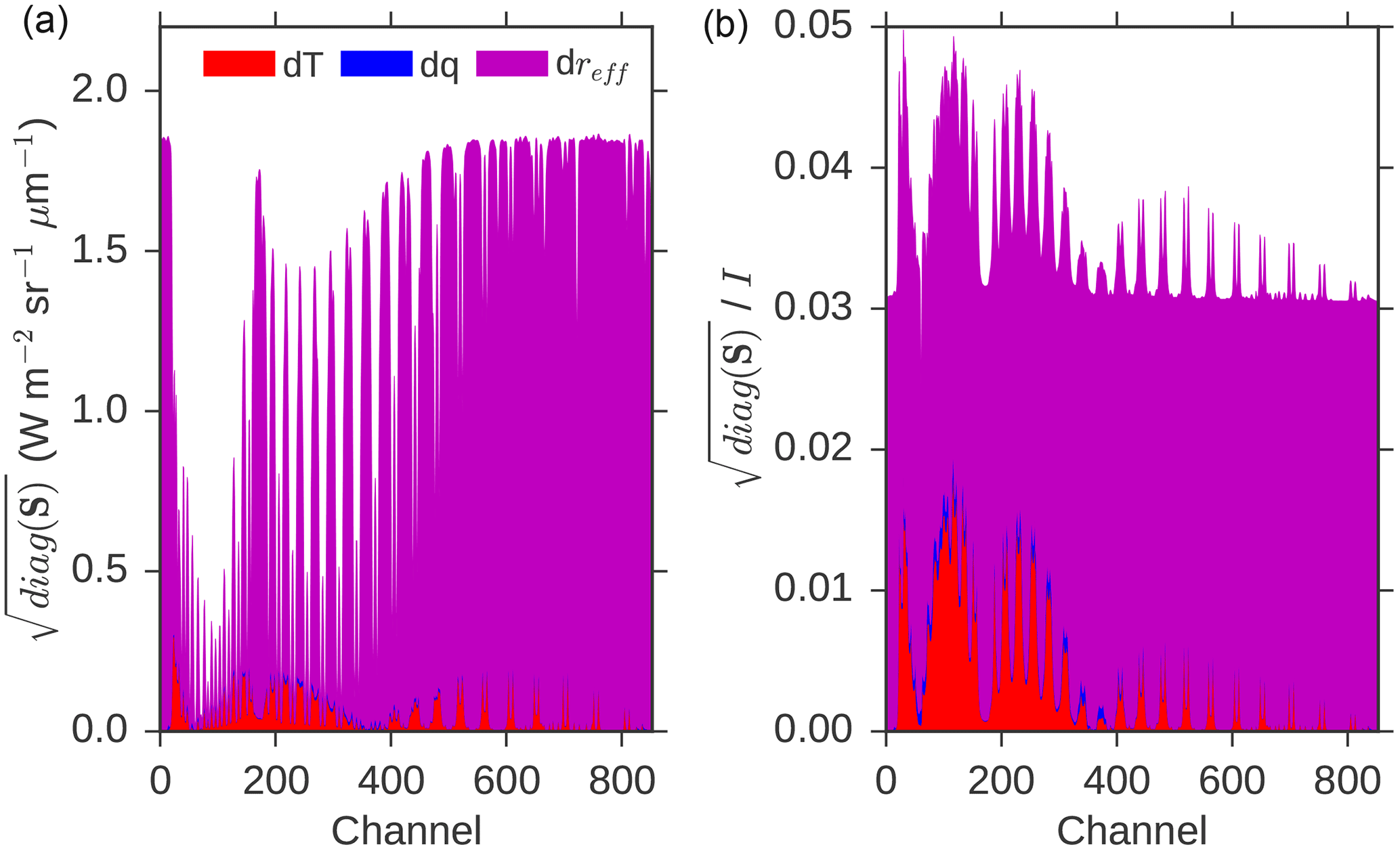
Figure 1Square root of diagonal components of the covariance matrix, stacked contribution from temperature (red), humidity (blue) and effective radius (magenta). Results shown for a cloud with τ = 10 and Ptop = 850 hPa. (a) Value in absolute radiance; (b) the same covariance values as a fraction of the unperturbed absolute radiance in the appropriate channel, such that 0.03 represents an uncertainty of ±3 %.
Figure 3 shows the relationship between the observation covariance matrix excluding the instrumental term SI for τ = 10, SZA = 30∘ and τ = 25, SZA = 60∘ with mid-latitude meteorology. Only the upper-diagonal elements of each matrix have been plotted to avoid duplication and values are scaled by , where μ0=cos θSZA. There is a linear relationship between the two matrices meaning that one may be reconstructed from the other. The results are similar for tropical and high-latitude cases, and for all soundings.
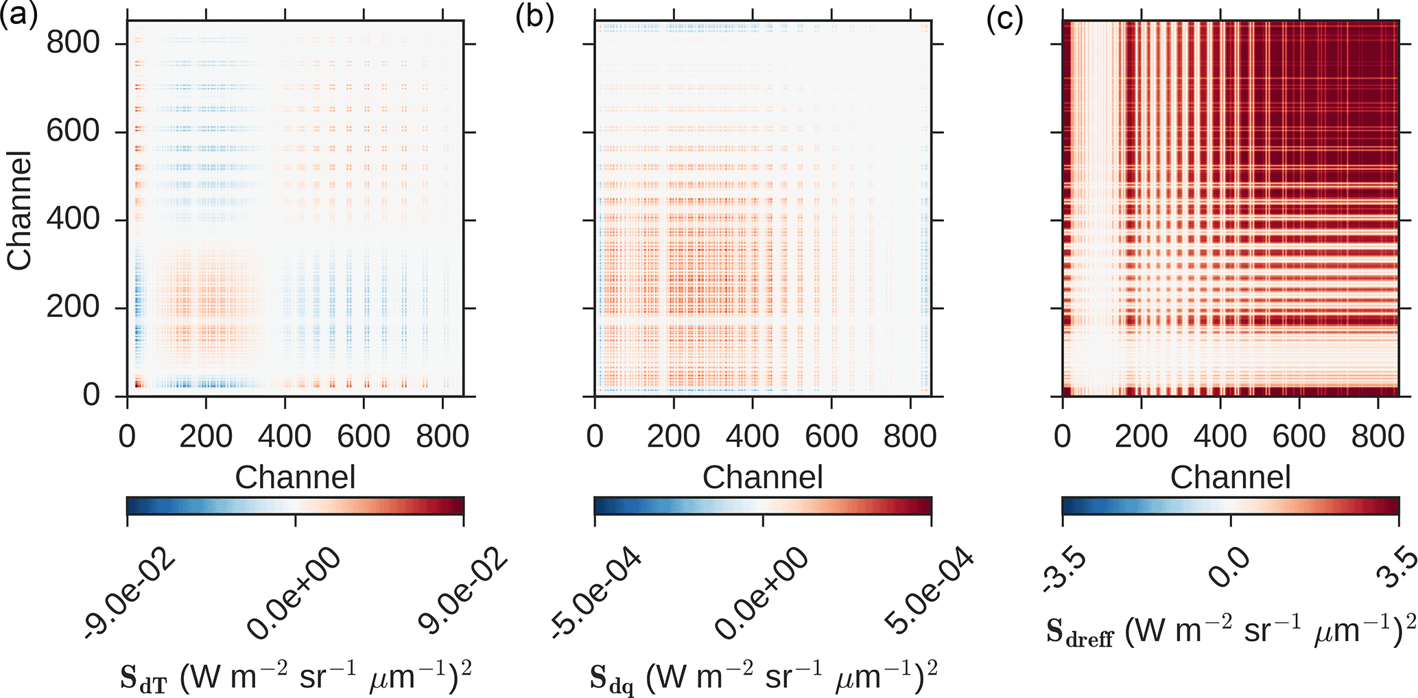
Figure 2Example covariance matrices for each component as labelled in the colour bar: (a) temperature, (b) humidity, and (c) effective radius.
4.1 Micro-window selection
Figure 4 shows IC and ds spectra using micro-windows consisting of 5, 75 or 200 OCO-2 channels. Also shown are the posterior errors in cloud properties taken from the square roots of the diagonal components of Sx.
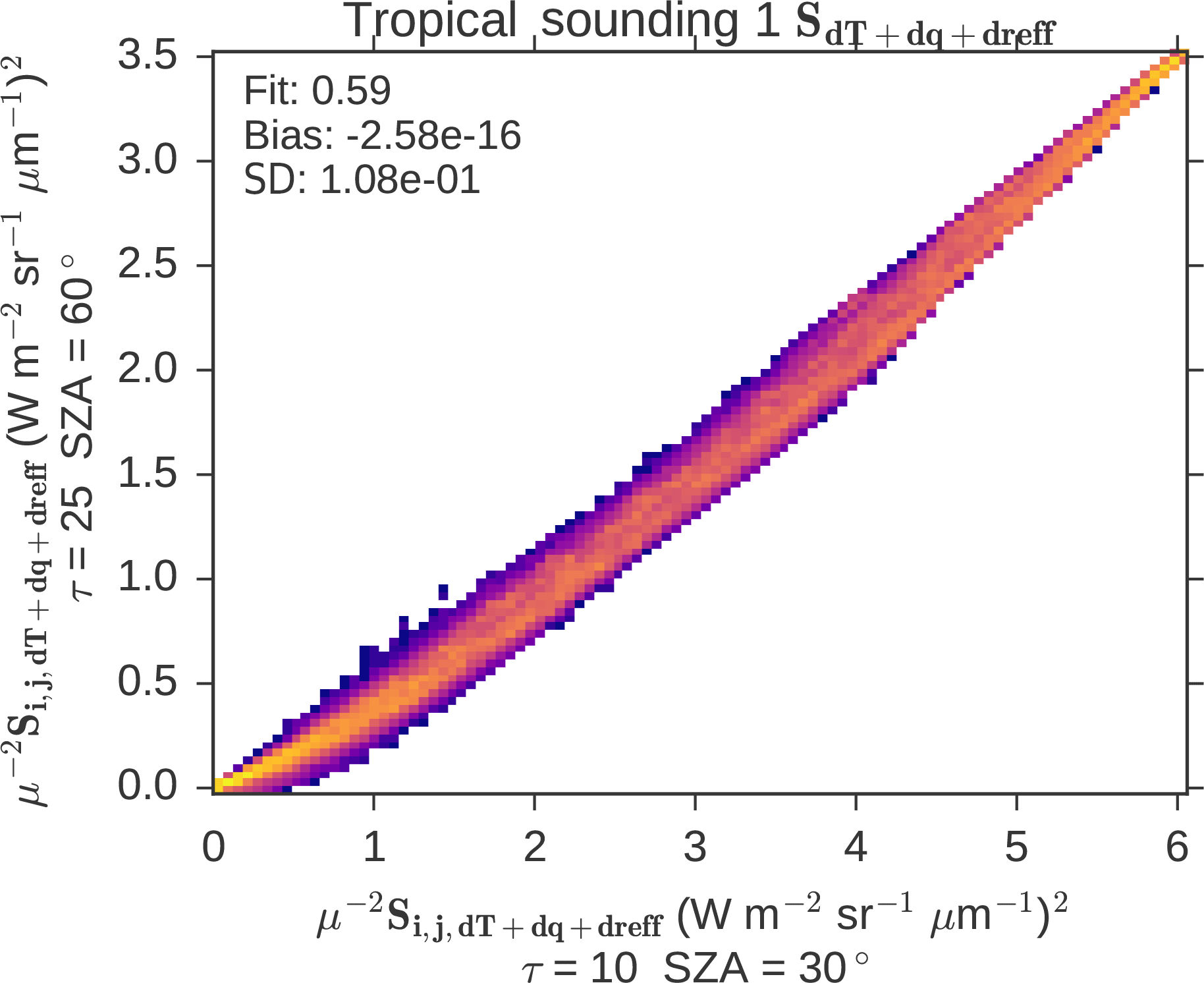
Figure 3Two-dimensional histograms of covariance matrix elements at 60∘ solar zenith angle as a function of the same values at 30∘ solar zenith angle for the mid-latitude meteorological state; each value has been scaled by to account for differences in illumination geometry.

Figure 4Results of information content analysis for a τ = 10 and Ptop = 850 hPa cloud in mean mid-latitude meteorology for OCO-2 sounding position 1. Each line represents the result using a micro-window of difference size, centred on the OCO-2 channel given in the x axis. Values are as follows: (a) information content in bits and (b) degrees of freedom for signal. Panels (c–e) show the square root of diagonal elements of posterior state covariance matrix: (c) cloud optical depth, (d) cloud-top pressure and (e) cloud pressure thickness.
In this cloud case (mid-latitude, τ = 10, Ptop = 850 hPa), the greatest information content comes from selecting channels near absorption features and avoiding the far wings of the A-band where only optical depth is reliably retrieved, as these channels have little O2 absorption and so are uninformative about photon path length. Otherwise, the five-channel micro-window is most sensitive to its placement within the spectrum: information content varies from 4.4 to 9.4 bit depending on the micro-window's location.
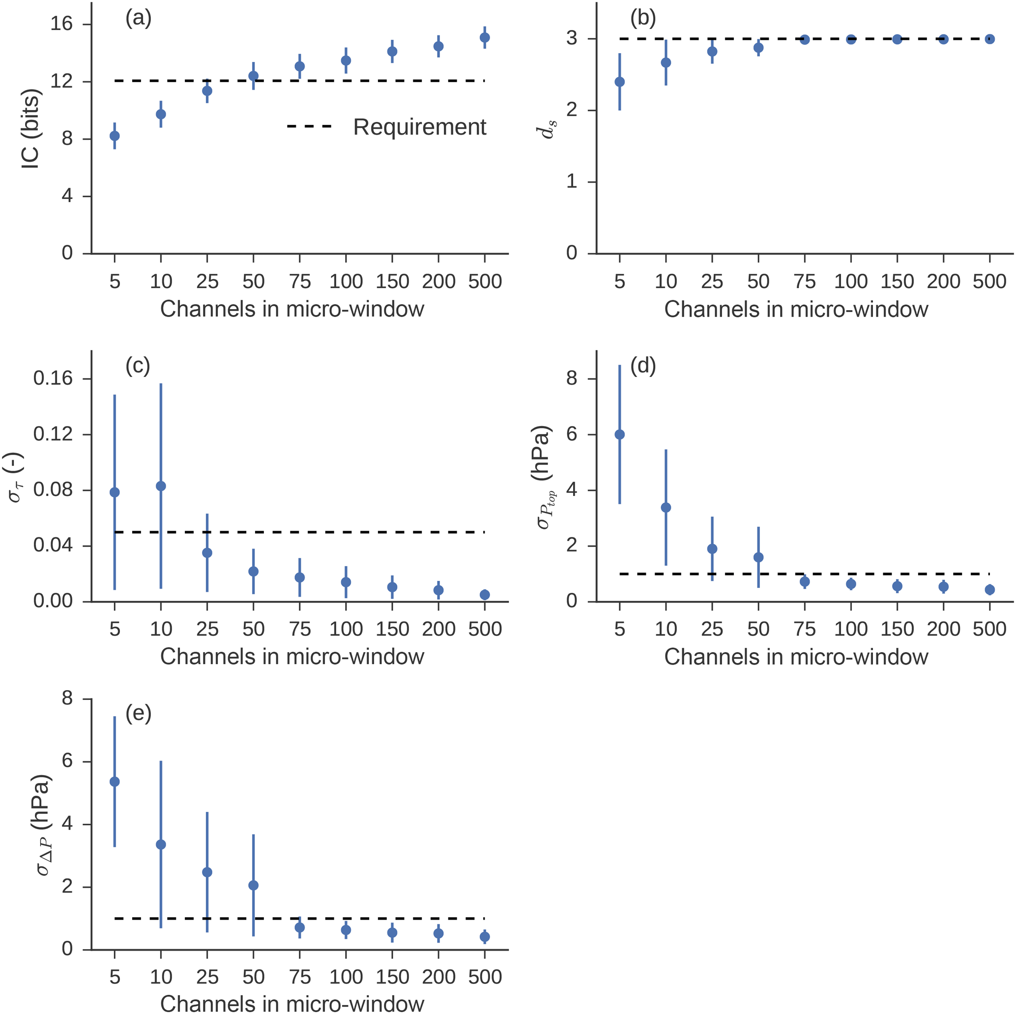
Figure 5Range of performance for best-located micro-window of each size. The point represents the central value and the lines the full range of the 216 outputs covering each sounding position, meteorology and cloud case. Note that the x axis is non-linear. (a) Information content in bits and (b) degrees of freedom for signal. Panels (c–e) show square root of diagonal covariance matrix elements: (c) cloud optical depth, (d) cloud-top pressure and (e) cloud pressure thickness. Dashed lines represent selected retrieval requirements.
Micro-windows that contain fewer channels are more sensitive to changes in the instrument line shapes and cloud conditions. For example, for the five-channel micro-window in Fig. 4, the best-performing channel has an information content of 9.4 bit. However, for a different cloudy case, τ = 25, Ptop = 680 hPa, and for sounding position 8 instead of 1, the information content is reduced to 6.0 bit. This is a substantial loss relative to the best possible micro-window for that cloud case, which has 8.4 bit of information.
To assess the relative trade-offs between increased speed and decreased performance we take the micro-window with the highest mean information content across all cases. We then plot the central value and full range of the 216 values for each selected micro-window size in Fig. 5, along with our chosen thresholds as dashed lines in each panel. The median case in the 50-channel micro-window passes our IC threshold and in all cases passes the τ uncertainty threshold, but it has multiple cases that fail the Ptop and ΔPc thresholds. By contrast, the 75-channel micro-window containing the OCO-2 channels 353–426 (indices counting from one for the full 1016 OCO-2 L1bSc channels) consistently satisfies our Ptop and ΔPc criteria and reduces the full wavelength range from 759.2–771.8 to 763.5–764.6 nm.
Figure 6 shows an example cloudy scene spectrum simulated for OCO-2 and highlights the chosen 75-channel micro-window in red. Also shown is an approximated GOME-2 spectrum based on the MetOp-B instrument characteristics (Munro et al., 2016). We approximate the ILS using Gaussian instrument line shapes, taking the 0.21 nm spectral sampling from Table 1 and FWHM of 0.50 nm from Table 2 of Munro et al. (2016). While OCO-2 spectra allow three independent pieces of information to be obtained (see the reported ds in the figure caption) our calculations agree with previous work that the GOME-2 resolution only provides approximately two (Schuessler et al., 2014). Consistent with older theoretical work (Heidinger and Stephens, 2000; O'Brien and Mitchell, 1992) this analysis supports the case the high spectral resolution of OCO-2 leads to additional information about cloud geometric thickness.
4.2 Theoretical retrieval case
Example synthetic retrieval iterations using the 75-channel micro-window are shown in Fig. 7 for τ=10 and τ=25 cases, and convergence typically occurs within a few iterations. Lines are coloured according to their χ2 values and it is clear that these are larger for cases where the result settles away from the true state. The posterior sample standard deviations are presented in Table 1 for the full samples and for cases where we filter the results by excluding the 10 % of cases with the highest χ2 in each case. The greatest effect of filtering by χ2 is to reduce the uncertainty in the cloud-top pressure and cloud pressure thickness from 12.9 to 2.9 and 2.5 hPa respectively. The mean standard deviation in the τ retrieval is ±0.75 across all cases, but this is inflated by a large value in the τ = 35 cases.

Figure 6Example simulated cloudy scene A-band spectrum, for a τ = 10, Ptop = 850 hPa cloud in a tropical atmosphere with a solar zenith angle of 45∘. The black line shows the full OCO-2 simulated spectrum, the blue line is the black line resampled using approximate GOME-2 instrument line shapes and the red line is the selected 75-channel micro-window for OCO-2 cloud retrievals. The legend also reports the ds for each spectrum with the GOME-2 instrumental uncertainty based on an SNR of 100 as in previous work (Schuessler et al., 2014).
Table 1Posterior errors estimated from the sample standard deviations of the retrieval output. In each case, σ refers to the full sample standard deviation and σ (filtered) refers to the sample standard deviation excluding those with the 10 % highest values of χ2. The bottom row shows the mean of the standard deviations entered in each row.
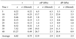
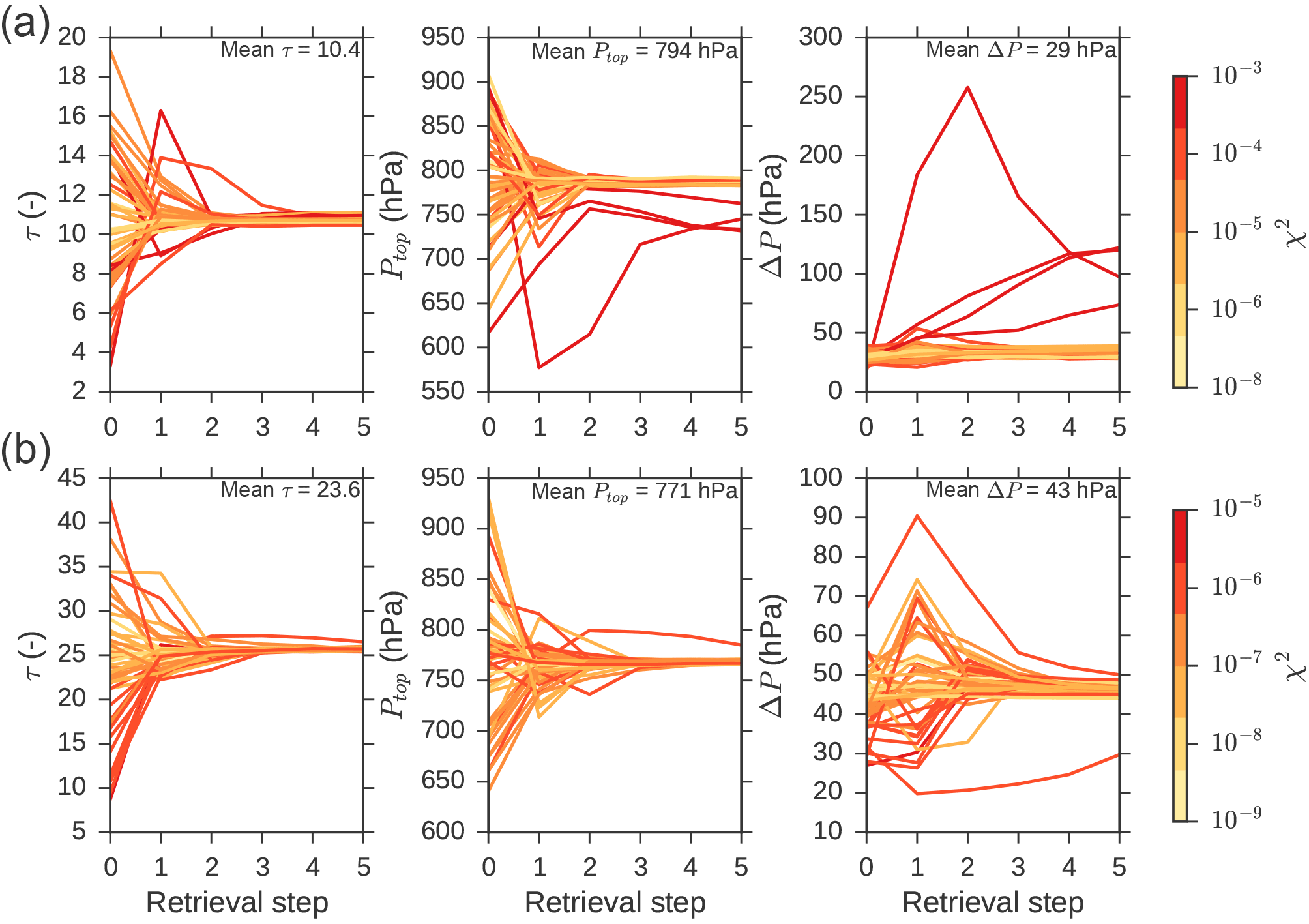
Figure 7Example iteration in retrieved cloud properties for synthetic micro-window retrievals for test cases with cloud optical depth near 10 (a) and 25 (b). Each line represents the iterations through 1 of the 50 sample retrievals. The lines are coloured according to their χ2 values; note the separate colour bars for the top and bottom rows with larger χ2 for the top cases.
OCO-2 O2 A-band spectra are rich in information about cloud properties. Continuum channels with little absorption respond strongly to cloud optical depth, while the radiance in absorption bands is dominated by photon path length, which increases with cloud-top pressure or cloud pressure thickness. A channel's response to cloud properties depends largely on its oxygen absorption coefficient (Fischer and Grassl, 1991; Koelemeijer et al., 2001; Stephens and Heidinger, 2000), and since many channels have similar absorption coefficients there is redundant cloud information in OCO-2 spectra.
We ultimately selected 75 neighbouring channels as containing the majority of the cloud information. Observation covariance matrices were developed based on uncertainty related to the atmospheric temperature and humidity profiles, in cloud droplet effective radius and instrumental uncertainty. These covariances depend on the meteorological profile, solar zenith angle and cloud properties. Additionally, instrument line shapes vary across the OCO-2 swath, so a separate covariance matrix is required for each of the eight across-track OCO-2 footprints. Fortunately, when cloud or meteorological properties change, the covariance matrix elements tend to be approximately linearly related, so an arbitrary covariance matrix can be reconstructed from a known case. There is greater spread in the reconstructed humidity component but this contributes a small fraction of the total covariance, which is dominated by uncertainty in the droplet radius whose component is well reconstructed.
Using 75 channels substantially reduces the retrieval processing time relative to the 853 available channels, and its usefulness was demonstrated in a set of eight synthetic test cases where a known cloud case was retrieved. In our perturbed tests the retrieval typically converged within two iterations, although a few cases converged on a local optimum instead of approaching the truth. Fortunately, these cases can generally be identified from the associated χ2, indicating that when this approach is applied to real OCO-2 data, it may be possible to flag cases where there is less confidence in the retrieval.
Our idealised posterior errors of ±0.75 in optical depth and better than ±3 hPa in cloud-top pressure and cloud pressure thickness are based on assuming that convergence can be identified from the χ2 values, and that the cloud is single-layered and horizontally homogeneous within the OCO-2 field of view of approximately 1.4 km × 2.2 km. This is a reasonable approximation in marine stratocumulus decks, where the typical length scale of variability in LWP can be 10–30 km (Wood and Hartmann, 2006), but will be violated in many low-level cloud cases such as at the edges of the stratocumulus–trade cumulus transition.
In addition, the assumption of a single scattering layer is commonly broken: multi-layered clouds are ubiquitous (Li et al., 2015), although for overlying cirrus it may be possible to identify and flag many of these cases based on the inferred distribution of photon path lengths from A-band measurements (Min et al., 2004). Alternatively, since OCO-2 flies in the A-Train it would also be possible to use other sensors such as CALIPSO (which is now leaving the A-Train) or MODIS to identify multi-layer cloud cases, or scenes in which there is heavy aerosol loading. Cases of heavy aerosol loading are most common over the Namibian stratocumulus region with common occurrence in June–July–August (JJA) and a peak in September–October–November (SON). A combination of CALIPSO, CloudSat and International Satellite Cloud Climatology Project (ISCCP) data imply that in the SON Namibian stratocumulus region, approximately one-third of low clouds have overlying aerosol, and approximately half of these cases are smoke (Devasthale and Thomas, 2011; Winker et al., 2010). Scattering layers overlying a marine cloud tend to reduce the effective retrieved cloud layer pressure due to the reduced mean path length of those photons reflected from the overlying layer (Vanbauce et al., 1998). Assessment of aerosol effects will be necessary in future work.
It was also assumed that the clouds will be reliably identified as liquid, and that a constant effective droplet size may be assumed. Droplet size variance has been included in terms of the observation covariance, but this limits our retrieved posterior covariance. Cloud identification is relatively simple for nadir A-band reflectance measurements over ocean, as for most solar zenith angles the surface is dark and cloudy scenes may simply be identified when reflectance exceeds some threshold. The OCO-2 instrument also carries weak and strong CO2 band spectrometers, and with ice absorbing more strongly than water in the near infrared we will be able to use well-known retrieval principles to obtain cloud phase (Nakajima and King, 1990).
Our assumptions mean that the true error of a cloud retrieval based on OCO-2 will be larger than that reported here, but our results suggest that the use of a 75-channel micro-window is justified as the basis of an OCO-2 cloud retrieval for marine liquid cloud properties.
The OCO-2 satellite carries an O2 A-band spectroradiometer with high spectral sampling. Our analysis supports that this spectral sampling is sufficient to, in principle, allow determination of the optical depth, cloud-top pressure and geometric pressure thickness of clouds. It has been demonstrated that observed OCO-2 spectra respond largely as expected to changes in cloud optical depth and cloud-top pressure (Richardson et al., 2017), but that study did not use modern Bayesian techniques. Such techniques account for relevant conditions such as line broadening due to local meteorology, and they also account for prior information and cross-correlation between the responses of individual channels.
Here we report that the OCO-2 A-band spectra contain much redundant information as a number of channels experience similar oxygen absorption. After accounting for observational errors associated with uncertainty introduced by meteorology, cloud droplet size and instrumental error, it was found that with a micro-window of 75 continuous channels, most of the information from the full 853-channel spectrum is retained. In a perfectly linear theoretical case, posterior error in cloud-top pressure and cloud pressure thickness were reduced below ±1 hPa and optical depth below ±0.05.
Using perturbed synthetic tests, the majority of cases approached the known truth and the full sample posterior errors averaged ±0.75 in optical depth and ±12.9 hPa in Ptop and cloud pressure thickness. Cases that converged to a state away from the truth could generally be identified by their large χ2 values, and removing the 10 % of worst cases reduced the posterior sample standard deviation in Ptop and ΔPc to ±2.9 and ±2.5 hPa.
These results apply in an ideal theoretical case of a uniform single-layer liquid droplet cloud, and retrieval errors will be larger in reality where these assumptions do not apply. However, violations of these assumptions such as real-world cloud heterogeneity will likely have a similar effect on both the full spectrum and on our selected 75-channel micro-window. We therefore propose that these assumptions do not affect our primary conclusion regarding the relative performance of our optimised retrieval versus a more intensive, full-spectrum retrieval.
The OCO-2 science data are available online from the NASA Goddard GES DISC at https://disc.gsfc.nasa.gov/datasets/OCO2_L1B_Science_V8r/summary (OCO-2 Science Team et al., 2017). The radiative transfer code is available from github at https://github.com/nasa/RtRetrievalFramework.
The authors declare that they have no conflict of interest.
The research described in this paper was performed
at the Jet Propulsion Laboratory, California Institute of Technology,
sponsored by NASA. Mark Richardson was funded by the OCO-2 and CloudSat projects. Mark Richardson
would like to thank James McDuffie and Jussi Leinonen for providing
radiative transfer and optimal estimation code assistance, plus Matt Lebsock, Annmarie Eldering, Mike Gunson, Chris O'Dell,
Tommy Taylor, Heather Cronk and Aronne Merrelli for helpful technical discussions.
Edited by: Alexander Kokhanovsky
Reviewed by: four anonymous referees
Baum, B. A., Menzel, W. P., Frey, R. A., Tobin, D. C., Holz, R. E., Ackerman, S. A., Heidinger, A. K., and Yang, P.: MODIS Cloud-Top Property Refinements for Collection 6, J. Appl. Meteorol. Clim., 51, 1145–1163, https://doi.org/10.1175/JAMC-D-11-0203.1, 2012.
Bennartz, R.: Global assessment of marine boundary layer cloud droplet number concentration from satellite, J. Geophys. Res., 112, D02201, https://doi.org/10.1029/2006JD007547, 2007.
Boesch, H., Brown, L., Castano, R., Christi, M., Connor, B., Crisp, D., Eldering, A., Fisher, B., Frankenberg, C., Gunson, M., Granat, R., McDuffie, J., Miller, C., Natraj, V., O'Brien, D., O'Dell, C., Osterman, G., Oyafuso, F., Payne, V., Polonsky, I., Smyth, M., Spurr, R., Thompson, D., and Toon, G.: Orbiting Carbon Observatory (OCO)-2 Level 2 Full Physics Algorithm Theoretical Basis Document, Pasadena, CA, available at: https://disc.gsfc.nasa.gov/OCO-2/documentation/oco-2-v6/OCO2_L2_ATBD.V6.pdf (last access: 5 March 2018), 2015.
Bony, S. and Dufresne, J.-L.: Marine boundary layer clouds at the heart of tropical cloud feedback uncertainties in climate models, Geophys. Res. Lett., 32, L20806, https://doi.org/10.1029/2005GL023851, 2005.
Borg, L. A. and Bennartz, R.: Vertical structure of stratiform marine boundary layer clouds and its impact on cloud albedo, Geophys. Res. Lett., 34, L05807, https://doi.org/10.1029/2006GL028713, 2007.
Brenguier, J.: Parameterization of the Condensation Process: A Theoretical Approach, J. Atmos. Sci., 48, 264–282, https://doi.org/10.1175/1520-0469(1991)048<0264:POTCPA>2.0.CO;2, 1991.
Chang, K.-W., L'Ecuyer, T. S., Kahn, B. H., and Natraj, V.: Information content of visible and midinfrared radiances for retrieving tropical ice cloud properties, J. Geophys. Res.-Atmos., 122, 4944–4966, https://doi.org/10.1002/2016JD026357, 2017.
Crisp, D.: NASA Orbiting Carbon Observatory: measuring the column averaged carbon dioxide mole fraction from space, J. Appl. Remote Sens., 2, 23508, https://doi.org/10.1117/1.2898457, 2008.
Crisp, D., Pollock, H. R., Rosenberg, R., Chapsky, L., Lee, R. A. M., Oyafuso, F. A., Frankenberg, C., O'Dell, C. W., Bruegge, C. J., Doran, G. B., Eldering, A., Fisher, B. M., Fu, D., Gunson, M. R., Mandrake, L., Osterman, G. B., Schwandner, F. M., Sun, K., Taylor, T. E., Wennberg, P. O., and Wunch, D.: The on-orbit performance of the Orbiting Carbon Observatory-2 (OCO-2) instrument and its radiometrically calibrated products, Atmos. Meas. Tech., 10, 59–81, https://doi.org/10.5194/amt-10-59-2017, 2017.
Deschamps, P.-Y., Breon, F.-M., Leroy, M., Podaire, A., Bricaud, A., Buriez, J.-C., and Seze, G.: The POLDER mission: instrument characteristics and scientific objectives, IEEE T. Geosci. Remote, 32, 598–615, https://doi.org/10.1109/36.297978, 1994.
Desmons, M., Ferlay, N., Parol, F., Mcharek, L., and Vanbauce, C.: Improved information about the vertical location and extent of monolayer clouds from POLDER3 measurements in the oxygen A-band, Atmos. Meas. Tech., 6, 2221–2238, https://doi.org/10.5194/amt-6-2221-2013, 2013.
Devasthale, A. and Thomas, M. A.: A global survey of aerosol-liquid water cloud overlap based on four years of CALIPSO-CALIOP data, Atmos. Chem. Phys., 11, 1143–1154, https://doi.org/10.5194/acp-11-1143-2011, 2011.
Ding, S., Wang, J., and Xu, X.: Polarimetric remote sensing in oxygen A and B bands: sensitivity study and information content analysis for vertical profile of aerosols, Atmos. Meas. Tech., 9, 2077–2092, https://doi.org/10.5194/amt-9-2077-2016, 2016.
Divakarla, M. G., Barnet, C. D., Goldberg, M. D., McMillin, L. M., Maddy, E., Wolf, W., Zhou, L., and Liu, X.: Validation of Atmospheric Infrared Sounder temperature and water vapor retrievals with matched radiosonde measurements and forecasts, J. Geophys. Res., 111, D09S15, https://doi.org/10.1029/2005JD006116, 2006.
Eldering, A., O'Dell, C. W., Wennberg, P. O., Crisp, D., Gunson, M. R., Viatte, C., Avis, C., Braverman, A., Castano, R., Chang, A., Chapsky, L., Cheng, C., Connor, B., Dang, L., Doran, G., Fisher, B., Frankenberg, C., Fu, D., Granat, R., Hobbs, J., Lee, R. A. M., Mandrake, L., McDuffie, J., Miller, C. E., Myers, V., Natraj, V., O'Brien, D., Osterman, G. B., Oyafuso, F., Payne, V. H., Pollock, H. R., Polonsky, I., Roehl, C. M., Rosenberg, R., Schwandner, F., Smyth, M., Tang, V., Taylor, T. E., To, C., Wunch, D., and Yoshimizu, J.: The Orbiting Carbon Observatory-2: first 18 months of science data products, Atmos. Meas. Tech., 10, 549–563, https://doi.org/10.5194/amt-10-549-2017, 2017.
Ferlay, N., Thieuleux, F., Cornet, C., Davis, A. B., Dubuisson, P., Ducos, F., Parol, F., Riédi, J., and Vanbauce, C.: Toward New Inferences about Cloud Structures from Multidirectional Measurements in the Oxygen A Band: Middle-of-Cloud Pressure and Cloud Geometrical Thickness from POLDER-3/PARASOL, J. Appl. Meteorol. Clim., 49, 2492–2507, https://doi.org/10.1175/2010JAMC2550.1, 2010.
Fischer, J. and Grassl, H.: Detection of Cloud-Top Height from Backscattered Radiances within the Oxygen A Band. Part 1: Theoretical Study, J. Appl. Meteorol., 30, 1245–1259, https://doi.org/10.1175/1520-0450(1991)030<1245:DOCTHF>2.0.CO;2, 1991.
Flatau, P. J. and Stephens, G. L.: On the fundamental solution of the radiative transfer equation, J. Geophys. Res., 93, 11037, https://doi.org/10.1029/JD093iD09p11037, 1988.
Frankenberg, C., O'Dell, C., Berry, J., Guanter, L., Joiner, J., Köhler, P., Pollock, R., and Taylor, T. E.: Prospects for chlorophyll fluorescence remote sensing from the Orbiting Carbon Observatory-2, Remote Sens. Environ., 147, 1–12, https://doi.org/10.1016/j.rse.2014.02.007, 2014.
Hanel, R. A.: Determination of cloud altitude from a satellite, J. Geophys. Res., 66, 1300–1300, https://doi.org/10.1029/JZ066i004p01300, 1961.
Heidinger, A. K. and Stephens, G. L.: Molecular Line Absorption in a Scattering Atmosphere. Part II: Application to Remote Sensing in the O2 A band, J. Atmos. Sci., 57, 1615–1634, https://doi.org/10.1175/1520-0469(2000)057<1615:MLAIAS>2.0.CO;2, 2000.
Herman, B. M.: Infra-red absorption, scattering, and total attenuation cross-sections for water spheres, Q. J. Roy. Meteor. Soc., 88, 143–150, https://doi.org/10.1002/qj.49708837604, 1962.
Huang, Y., Siems, S. T., Manton, M. J., Hande, L. B., and Haynes, J. M.: The Structure of Low-Altitude Clouds over the Southern Ocean as Seen by CloudSat, J. Climate, 25, 2535–2546, https://doi.org/10.1175/JCLI-D-11-00131.1, 2012.
Koelemeijer, R. B. A., Stammes, P., Hovenier, J. W., and de Haan, J. F.: A fast method for retrieval of cloud parameters using oxygen A band measurements from the Global Ozone Monitoring Experiment, J. Geophys. Res.-Atmos., 106, 3475–3490, https://doi.org/10.1029/2000JD900657, 2001.
L'Ecuyer, T. S. and Jiang, J. H.: Touring the atmosphere aboard the A-Train, Phys. Today, 63, 36–41, https://doi.org/10.1063/1.3463626, 2010.
Li, J., Huang, J., Stamnes, K., Wang, T., Lv, Q., and Jin, H.: A global survey of cloud overlap based on CALIPSO and CloudSat measurements, Atmos. Chem. Phys., 15, 519–536, https://doi.org/10.5194/acp-15-519-2015, 2015.
Mahfouf, J.-F., Birman, C., Aires, F., Prigent, C., Orlandi, E., and Milz, M.: Information content on temperature and water vapour from a hyper-spectral microwave sensor, Q. J. Roy. Meteor. Soc., 141, 3268–3284, https://doi.org/10.1002/qj.2608, 2015.
Martinet, P., Lavanant, L., Fourrié, N., Rabier, F. and Gambacorta, A.: Evaluation of a revised IASI channel selection for cloudy retrievals with a focus on the Mediterranean basin, Q. J. Roy. Meteor. Soc., 140, 1563–1577, https://doi.org/10.1002/qj.2239, 2014.
Merlin, G., Riedi, J., Labonnote, L. C., Cornet, C., Davis, A. B., Dubuisson, P., Desmons, M., Ferlay, N., and Parol, F.: Cloud information content analysis of multi-angular measurements in the oxygen A-band: application to 3MI and MSPI, Atmos. Meas. Tech., 9, 4977–4995, https://doi.org/10.5194/amt-9-4977-2016, 2016.
Miles, N. L., Verlinde, J., and Clothiaux, E. E.: Cloud Droplet Size Distributions in Low-Level Stratiform Clouds, J. Atmos. Sci., 57, 295–311, https://doi.org/10.1175/1520-0469(2000)057<0295:CDSDIL>2.0.CO;2, 2000.
Min, Q.-L., Harrison, L. C., Kiedron, P., Berndt, J., and Joseph, E.: A high-resolution oxygen A-band and water vapor band spectrometer, J. Geophys. Res., 109, D02202, https://doi.org/10.1029/2003JD003540, 2004.
Munro, R., Lang, R., Klaes, D., Poli, G., Retscher, C., Lindstrot, R., Huckle, R., Lacan, A., Grzegorski, M., Holdak, A., Kokhanovsky, A., Livschitz, J., and Eisinger, M.: The GOME-2 instrument on the Metop series of satellites: instrument design, calibration, and level 1 data processing – an overview, Atmos. Meas. Tech., 9, 1279–1301, https://doi.org/10.5194/amt-9-1279-2016, 2016.
Nakajima, T. and King, M. D.: Determination of the Optical Thickness and Effective Particle Radius of Clouds from Reflected Solar Radiation Measurements. Part I: Theory, J. Atmos. Sci., 47, 1878–1893, https://doi.org/10.1175/1520-0469(1990)047<1878:DOTOTA>2.0.CO;2, 1990.
Natraj, V. and Spurr, R. J. D.: A fast linearized pseudo-spherical two orders of scattering model to account for polarization in vertically inhomogeneous scattering–absorbing media, J. Quant. Spectrosc. Ra., 107, 263–293, https://doi.org/10.1016/j.jqsrt.2007.02.011, 2007.
O'Brien, D. M. and Mitchell, R. M.: Error Estimates for Retrieval of Cloud-Top Pressure Using Absorption in the A Band of Oxygen, J. Appl. Meteorol., 31, 1179–1192, https://doi.org/10.1175/1520-0450(1992)031<1179:EEFROC>2.0.CO;2, 1992.
OCO-2 Science Team, Gunson, M., and Eldering, A.: OCO-2 Level 1B calibrated, geolocated science spectra, Retrospective Processing V8r, Greenbelt, MD, USA, Goddard Earth Sciences Data and Information Services Center (GES DISC), https://doi.org/10.5067/1RJW1YMLW2F0, 2017.
O'Dell, C. W.: Acceleration of multiple-scattering, hyperspectral radiative transfer calculations via low-streams interpolation, J. Geophys. Res., 115, D10206, https://doi.org/10.1029/2009JD012803, 2010.
Osterman, G. B., Eldering, A., Avis, C., Chafin, B., O'Dell, C. W., Frankenberg, C., Fisher, B. M., Mandrake, L., Wunch, D., Granat, R., and Crisp, D.: Orbiting Carbon Observatory-2 (OCO-2) Data Product User's Guide, Operational L1 and L2 Data Versions 7 and 7R, Jet Propulsion Laboratory, Pasadena, CA, USA, 2016.
Platnick, S., Ackerman, S. A., King, M. D., Meyer, K., Menzel, W. P., Holz, R. E., Baum, B. A., and Yang, P.: MODIS atmosphere L2 cloud product (06_L2), Goddard Space Flight Center, Greenbelt, MA, USA, https://doi.org/10.5067/MODIS/MYD06_L2.006, 2015.
Rabier, F., Fourrié, N., Chafaï, D., and Prunet, P.: Channel selection methods for Infrared Atmospheric Sounding Interferometer radiances, Q. J. Roy. Meteor. Soc., 128, 1011–1027, https://doi.org/10.1256/0035900021643638, 2002.
Richardson, M., McDuffie, J., Stephens, G. L., Cronk, H. Q., and Taylor, T. E.: The OCO-2 oxygen A-band response to liquid marine cloud properties from CALIPSO and MODIS, J. Geophys. Res.-Atmos., 122, 8255–8275, https://doi.org/10.1002/2017JD026561, 2017.
Rodgers, C. D.: Inverse Methods for Atmospheric Sounding Theory and Practice, World Scientific, Singapore, 2000.
Rozanov, V. V. and Kokhanovsky, A. A.: Semianalytical cloud retrieval algorithm as applied to the cloud top altitude and the cloud geometrical thickness determination from top-of-atmosphere reflectance measurements in the oxygen A band, J. Geophys. Res., 109, D05202, https://doi.org/10.1029/2003JD004104, 2004.
Schuessler, O., Loyola Rodriguez, D. G., Doicu, A., and Spurr, R.: Information Content in the Oxygen A-Band for the Retrieval of Macrophysical Cloud Parameters, IEEE T. Geosci. Remote, 52, 3246–3255, https://doi.org/10.1109/TGRS.2013.2271986, 2014.
Shannon, C. and Weaver, W.: The Mathematical Theory of Communication, Univ. of Illinois Press, Urbana, IL, USA, 1949.
Spurr, R. J. D.: VLIDORT: A linearized pseudo-spherical vector discrete ordinate radiative transfer code for forward model and retrieval studies in multilayer multiple scattering media, J. Quant. Spectrosc. Ra., 102, 316–342, https://doi.org/10.1016/j.jqsrt.2006.05.005, 2006.
Spurr, R. J. D., Kurosu, T. P., and Chance, K. V.: A linearized discrete ordinate radiative transfer model for atmospheric remote-sensing retrieval, J. Quant. Spectrosc. Ra., 68, 689–735, https://doi.org/10.1016/S0022-4073(00)00055-8, 2001.
Stephens, G. L.: Radiation Profiles in Extended Water Clouds. II: Parameterization Schemes, J. Atmos. Sci., 35, 2123–2132, https://doi.org/10.1175/1520-0469(1978)035<2123:RPIEWC>2.0.CO;2, 1978.
Stephens, G. L. and Heidinger, A.: Molecular Line Absorption in a Scattering Atmosphere. Part I: Theory, J. Atmos. Sci., 57, 1599–1614, https://doi.org/10.1175/1520-0469(2000)057<1599:MLAIAS>2.0.CO;2, 2000.
Stephens, G. L., Vane, D. G., Tanelli, S., Im, E., Durden, S., Rokey, M., Reinke, D., Partain, P., Mace, G. G., Austin, R., L'Ecuyer, T., Haynes, J., Lebsock, M., Suzuki, K., Waliser, D., Wu, D., Kay, J., Gettelman, A., Wang, Z., and Marchand, R.: CloudSat mission: Performance and early science after the first year of operation, J. Geophys. Res., 113, D00A18, https://doi.org/10.1029/2008JD009982, 2008.
Szczodrak, M., Austin, P. H., and Krummel, P. B.: Variability of Optical Depth and Effective Radius in Marine Stratocumulus Clouds, J. Atmos. Sci., 58, 2912–2926, https://doi.org/10.1175/1520-0469(2001)058<2912:VOODAE>2.0.CO;2, 2001.
Taylor, T. E., O'Dell, C. W., Frankenberg, C., Partain, P. T., Cronk, H. Q., Savtchenko, A., Nelson, R. R., Rosenthal, E. J., Chang, A. Y., Fisher, B., Osterman, G. B., Pollock, R. H., Crisp, D., Eldering, A., and Gunson, M. R.: Orbiting Carbon Observatory-2 (OCO-2) cloud screening algorithms: validation against collocated MODIS and CALIOP data, Atmos. Meas. Tech., 9, 973–989, https://doi.org/10.5194/amt-9-973-2016, 2016.
Vanbauce, C., Buriez, J. C., Parol, F., Bonnel, B., Sèze, G., and Couvert, P.: Apparent pressure derived from ADEOS-POLDER observations in the oxygen A-band over ocean, Geophys. Res. Lett., 25, 3159–3162, https://doi.org/10.1029/98GL02324, 1998.
Vaughan, M. A., Powell, K. A., Winker, D. M., Hostetler, C. A., Kuehn, R. E., Hunt, W. H., Getzewich, B. J., Young, S. A., Liu, Z., and McGill, M. J.: Fully Automated Detection of Cloud and Aerosol Layers in the CALIPSO Lidar Measurements, J. Atmos. Ocean. Tech., 26, 2034–2050, https://doi.org/10.1175/2009JTECHA1228.1, 2009.
Vidot, J., Bennartz, R., O'Dell, C. W., Preusker, R., Lindstrot, R., and Heidinger, A. K.: CO2 Retrieval over Clouds from the OCO Mission: Model Simulations and Error Analysis, J. Atmos. Ocean. Tech., 26, 1090–1104, https://doi.org/10.1175/2009JTECHA1200.1, 2009.
Winker, D. M., Pelon, J., Coakley, J. A., Ackerman, S. A., Charlson, R. J., Colarco, P. R., Flamant, P., Fu, Q., Hoff, R. M., Kittaka, C., Kubar, T. L., Le Treut, H., McCormick, M. P., Mégie, G., Poole, L., Powell, K., Trepte, C., Vaughan, M. A., and Wielicki, B. A.: The CALIPSO Mission: A Global 3D View of Aerosols and Clouds, B. Am. Meteorol. Soc., 91, 1211–1229, https://doi.org/10.1175/2010BAMS3009.1, 2010.
Wood, R. and Hartmann, D. L.: Spatial Variability of Liquid Water Path in Marine Low Cloud: The Importance of Mesoscale Cellular Convection, J. Climate, 19, 1748–1764, https://doi.org/10.1175/JCLI3702.1, 2006.
Yamamoto, G. and Wark, D. Q.: Discussion of the letter by R. A. Hanel, “Determination of cloud altitude from a satellite”, J. Geophys. Res., 66, 3596–3596, https://doi.org/10.1029/JZ066i010p03596, 1961.
Yang, Y., Marshak, A., Mao, J., Lyapustin, A., and Herman, J.: A method of retrieving cloud top height and cloud geometrical thickness with oxygen A and B bands for the Deep Space Climate Observatory (DSCOVR) mission: Radiative transfer simulations, J. Quant. Spectrosc. Ra., 122, 141–149, https://doi.org/10.1016/j.jqsrt.2012.09.017, 2013.
Zelinka, M. D., Klein, S. A., and Hartmann, D. L.: Computing and Partitioning Cloud Feedbacks Using Cloud Property Histograms. Part I: Cloud Radiative Kernels, J. Climate, 25, 3715–3735, https://doi.org/10.1175/JCLI-D-11-00248.1, 2012.