the Creative Commons Attribution 4.0 License.
the Creative Commons Attribution 4.0 License.
 | 06 Apr 2018
The BErkeley Atmospheric CO2 Observation Network: field calibration and evaluation of low-cost air quality sensors
Jinsol Kim
Alexis A. Shusterman
Kaitlyn J. Lieschke
Catherine Newman
The newest generation of air quality sensors is small, low cost, and easy to deploy. These sensors are an attractive option for developing dense observation networks in support of regulatory activities and scientific research. They are also of interest for use by individuals to characterize their home environment and for citizen science. However, these sensors are difficult to interpret. Although some have an approximately linear response to the target analyte, that response may vary with time, temperature, and/or humidity, and the cross-sensitivity to non-target analytes can be large enough to be confounding. Standard approaches to calibration that are sufficient to account for these variations require a quantity of equipment and labor that negates the attractiveness of the sensors' low cost. Here we describe a novel calibration strategy for a set of sensors, including CO, NO, NO2, and O3, that makes use of (1) multiple co-located sensors, (2) a priori knowledge about the chemistry of NO, NO2, and O3, (3) an estimate of mean emission factors for CO, and (4) the global background of CO. The strategy requires one or more well calibrated anchor points within the network domain, but it does not require direct calibration of any of the individual low-cost sensors. The procedure nonetheless accounts for temperature and drift, in both the sensitivity and zero offset. We demonstrate this calibration on a subset of the sensors comprising BEACO2N, a distributed network of approximately 50 sensor “nodes”, each measuring CO2, CO, NO, NO2, O3 and particulate matter at 10 s time resolution and approximately 2 km spacing within the San Francisco Bay Area.


In urban environments, air quality has complex spatial and temporal patterns. Diverse emission sources are present with large variations in emission rate and source type on scales of hundreds of meters. In addition, dispersion of pollutants into the urban environment is affected by the topography of the urban landscape and the associated wind flows, which also vary on length scales of ∼ 100 m (Vardoulakis et al., 2003; Lateb et al., 2016). Conventional approaches to air quality monitoring rely on a limited number of relatively high-cost instruments that lack the spatial resolution needed to characterize these variations, opting instead to target spatial averages. This averaging hampers our attempts at source attribution and understanding of mixing, chemistry, and human exposure in cities where emissions vary on spatial scales that are small compared to typical observations or models.
One approach to obtaining higher spatial resolution observations is passive sampling, which has been implemented using inexpensive sampling devices that can be later analyzed in bulk. Passive samplers do not require electrical power to function properly and are collected and analyzed 1 to 2 weeks after deployment. Such protocols provide high spatial resolution but also have significant drawbacks. Spatial resolution is gained at the expense of temporal resolution, and analysis after collection of the samplers is time consuming; thus passive sampling has typically been used only in short-duration experiments (e.g., Krupa and Legge, 2000; Cox, 2003). Furthermore, as a result of boundary layer dynamics, passive sampling in urban areas is likely dominated by the high concentrations found at night and relatively insensitive to daytime variability.
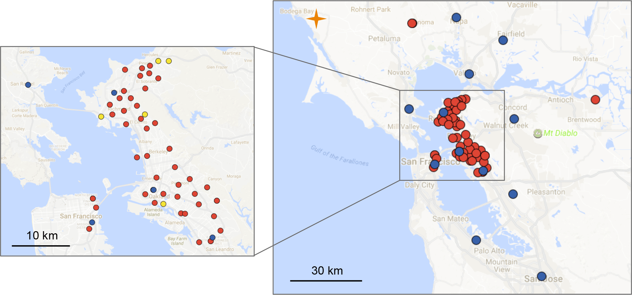
Figure 1Map of San Francisco Bay Area showing current BEACO2N node sites (red), BAAQMD reference sites with O3 measurements (blue), and the BAAQMD Bodega Bay regional greenhouse gas background site (orange). The sites used in this analysis are marked in yellow on the detailed panel.
Recent developments in low-cost sensors for trace gases and particulate matter, as well as advances in software and hardware enabling low-cost data communication, have made high-density, high-time-resolution air quality monitoring networks possible. Devices and networks of devices are emerging that are low cost, report at a time resolution of seconds, and are capable of long-term deployment, providing potential for improvement over the two major weaknesses of passive sampling. Examples include metal oxide sensors used to measure O3, CO, NO2, and total volatile organic compounds (e.g., Williams et al., 2013; Bart et al., 2014; Piedrahita et al., 2014; Moltchanov et al., 2015; Sadighi et al., 2017), and electrochemical sensors used to measure CO, NO, NO2, O3, and SO2 (e.g., Mead et al., 2013; Sun et al., 2015; Jiao et al., 2016; Hagan et al., 2017; Jerrett et al., 2017; Mueller et al., 2017). These different low-cost sensor systems have been evaluated and compared (Borrego et al., 2016; Papapostolou et al., 2017). While these studies found low-cost trace gas sensors to be successful at qualitatively characterizing the variability of air quality in an urban area, challenges related to selectivity and stability remain, hindering more quantitative interpretation of the data.
The current generation of low-cost sensors is not as easily tied to a gravimetric calibration standard as many of the passive samplers. Calibration is known to vary with sensor age, temperature, and in some cases humidity. In addition, many of the sensors have responses to gases other than the target analyte (Mead et al., 2013; Spinelle et al., 2015, 2017; Cross et al., 2017; Mueller et al., 2017; Mijling et al., 2018; Zimmerman et al., 2018). One approach to addressing this challenge is to combine periodic re-calibration and co-location with regulatory reference instruments in the lab or the field (Williams et al., 2013; Moltchanov et al., 2015; Jiao et al., 2016; Mijling et al., 2018). Field calibration is preferred as in-lab performance is often a poor approximation of sensor behavior under ambient conditions (Piedrahita et al., 2014; Masson et al., 2015). However, either method requires considerable time investment by trained personnel, especially as the number of sensors increases. The requirement of time-consuming and labor-intensive calibration then offsets the low-cost advantage of the sensors.
In this paper, we explore an automated, in situ strategy for the calibration of individual sensors embedded in an air quality sensor network that includes both low-cost sensors and anchor points of higher-grade, well-calibrated instrumentation. The BErkeley Atmospheric CO2 Observation Network (BEACO2N) is a low-cost, high-density greenhouse gas (CO2) and air quality (CO, NO, NO2, O3, and particulate matter) monitoring network located in San Francisco Bay Area, California (see Fig. 1 and Shusterman et al., 2016). As of this writing, BEACO2N consists of approximately 50 sensor “nodes”, deployed with approximately 2 km horizontal spacing. Most of the nodes are mounted on the roofs of schools and museums. In previous work, we described an approach to CO2 sensing and calibration (Shusterman et al., 2016). Here, we focus on CO, NO, NO2, and O3.
We begin by describing laboratory experiments and in-field comparisons to co-located reference instruments that give an initial characterization of the sensors and provide insight into the effects of temperature, humidity, and cross-sensitivity to non-target analytes. Then we describe an in situ calibration procedure that accounts for these variables without requiring co-location with a reference instrument. The calibration procedure is finally verified against regulatory quality measurements not used in the procedure itself.
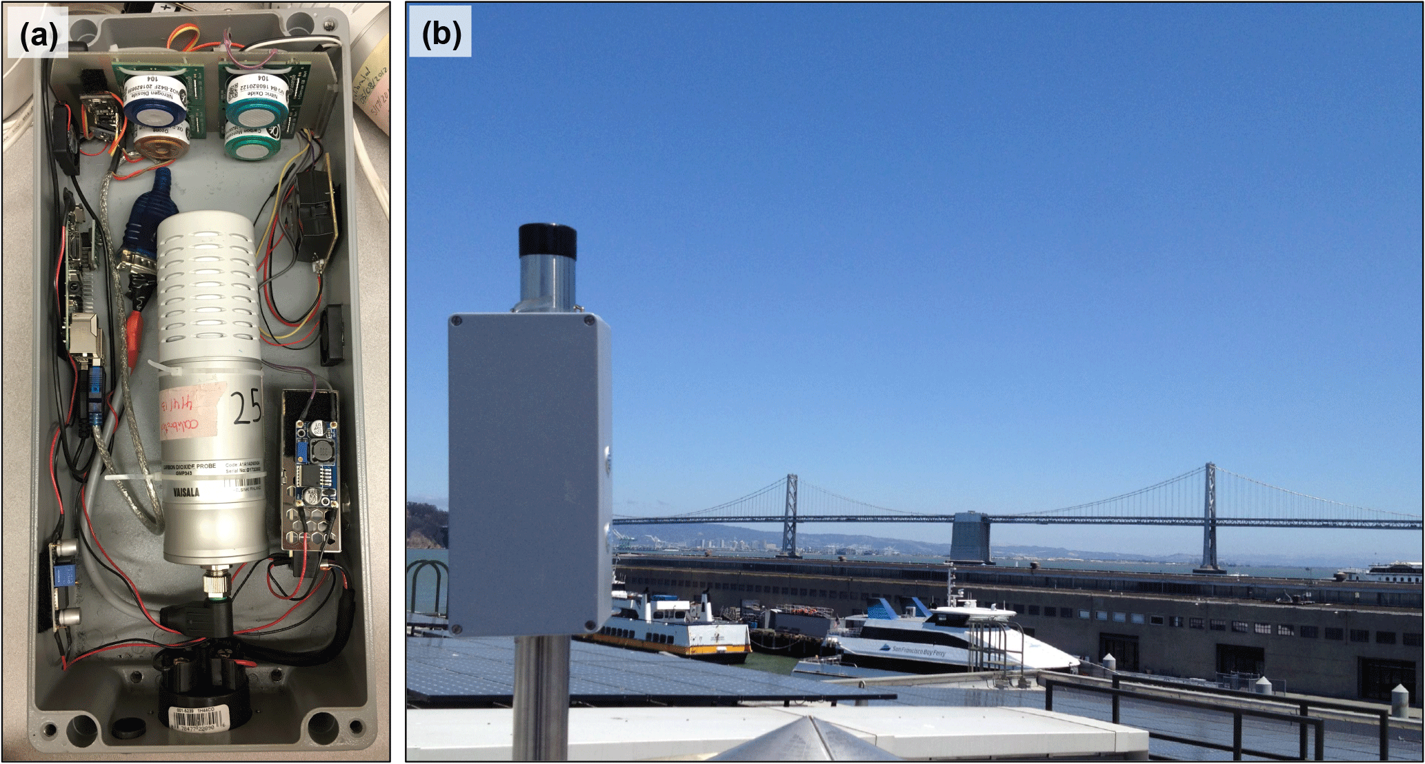
Details of the node design and deployment are described in Shusterman et al. (2016). Briefly, each BEACO2N node contains a Vaisala CarboCap GMP343 non-dispersive infrared sensor for CO2, a Shinyei PPD42NS nephelometric particulate matter sensor, and a suite of Alphasense electrochemical sensors: CO-B4, NO-B4, either NO2-B42F or NO2-B43F, and either Ox-B421 or Ox-B431. All sensors are assembled into compact, weatherproof enclosures as shown in Fig. 2. Two 30 mm fans are located on either side of the enclosure to facilitate airflow through the node. A Raspberry Pi microprocessor collects data via a serial-to-USB converter for CO2 and an Adafruit Metro Mini microcontroller for all other sensors. Then, data collected every 5 or 10 s are transmitted to a central server using a direct on-site Ethernet connection or a local Wi-Fi network.
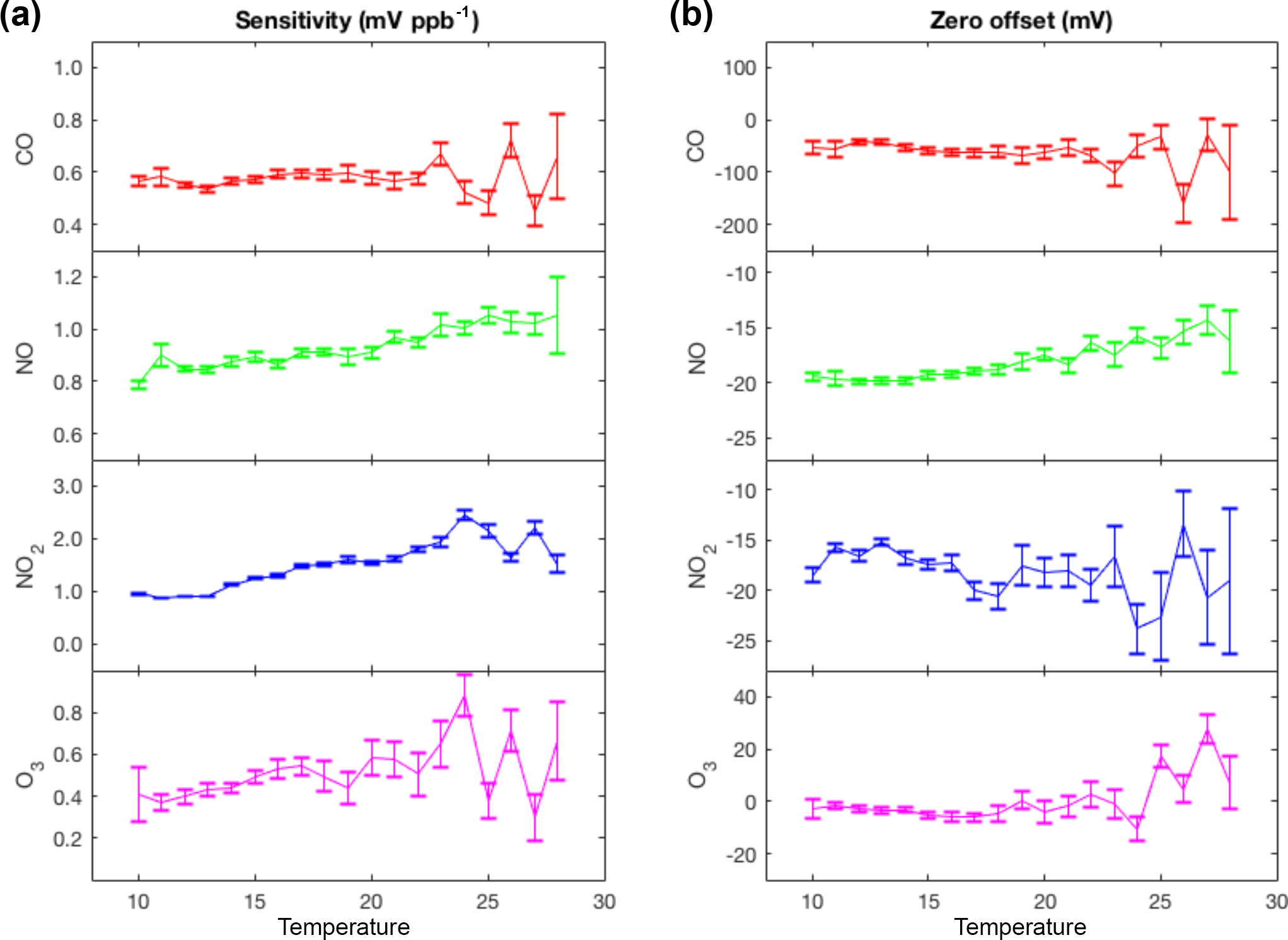
Figure 3Representative temperature-dependent sensitivities (a) and zero offsets (b) of the Alphasense electrochemical sensors calculated by comparing hourly averaged measurements from Laney College BEACO2N node to measurements from a co-located reference instrument during February to April 2016.
The Alphasense B4 electrochemical gas sensing series that we use employs a four-electrode approach. The electrodes are embedded in an electrolyte solution separated from the atmosphere by a semi-permeable membrane. The gas of interest diffuses through the membrane into the electrolyte, where it contacts a “working” electrode and is either oxidized (in the case of NO and CO) or reduced (NO2 and O3). The potential at the working electrode is maintained at a constant value with respect to a “reference” electrode. Electric charge produced at the working electrode is balanced by the complementary redox reaction at a “counter” electrode, generating an electric current. The sensor also contains an “auxiliary” electrode, which shares the working electrode's catalyst structure, but is isolated from the ambient environment, accounting for fluctuations in the background current associated with other processes at the electrode and electrolyte. Subtracting the auxiliary current from the working current gives a corrected current dependent on the gas concentration.
The working and auxiliary currents detected by the sensors are converted to working and auxiliary voltages using amplifiers in the individual sensor boards (ISBs) provided by Alphasense. Over the mixing ratio range of interest, the sensors' responses to the gases of interest are approximately linear. We derive mixing ratios from the observed voltages by subtracting an offset and then scaling by a constant (Eqs. 1–4):
Here, CO, NO, NO2, and O3 with the subscript “ambient” refer to the gas mixing ratios (ppb) in air; VCO, VNO, and are the signals (mV) measured by each sensor, which is the voltage of the auxiliary electrode subtracted from the voltage of the working electrode; zeroCO, zeroNO, zero and zero indicates the voltage measured in the absence of analyte; and kCO, kNO, and represent the linear sensitivity factor that converts mV to ppb. Additional terms corresponding to the cross-sensitivities of the NO2 and O3 sensors appear in Eqs. (3a), (3b), and (4), where is the cross-sensitivity of the NO2-B42F sensor to NO gas, is the cross-sensitivity of the NO2-B43F sensor to CO2 gas, and is the cross-sensitivity of both the O3-B421 and O3-B431 sensors to NO2 gas.
There are a total of eight sensitivities and zero offsets, as well as two cross-sensitivity terms. All of these may also vary with time, temperature, and humidity. Thus we need a calibration strategy that constrains 10 parameters in a single instant as well as the variation of those 10 parameters in response to the environmental variables and time. We begin by characterizing the sensors in both laboratory and outdoor environments.
We evaluate BEACO2N in terms of four factors: drift, noise, cross-sensitivity, and temperature dependence. The humidity dependence is included in the temperature dependence, as there is no evidence for independent humidity dependence and relative humidity exhibits an anti-correlation with temperature in the field. In the laboratory, a range of mixing ratios of target gases were delivered to a chamber containing the full suite of four Alphasense B4 sensors: CO, NO, NO2, and O3. Zero air was supplied by a Sabio 1001 compressed zero-air source and blended with calibration gases using a Thermo Scientific model 146i multi-gas calibrator.
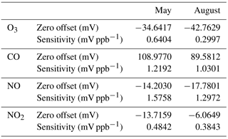
Table 1Zero offsets and sensitivities of a representative quartet of Alphasense B4 electrochemical sensors derived via comparison to delivered reference gases during two separate laboratory calibration separated by an approximately 10-week interlude.
Noise. Alphasense reports 2σ noise of ±4, ±15, ±12, and ±15 ppb for CO, NO, NO2, and O3, respectively over concentrations from 0 to 200 ppb at time resolution of a second. In our laboratory, noise (±2σ) was measured for ambient ppb levels with 10 s time resolution and was seen to be ±10 ppb for CO, ±3 ppb for NO, ±6 ppb for NO2 (NO2-B42F and NO2-B43F), and ±12 ppb for O3 (O3-B421 and O3-B431).
Cross-sensitivity. We measured the cross-sensitivity of all four of the trace gas sensors to the non-target gases. The NO2 sensors and O3 sensors were the only ones to exhibit sensitivity to other species. The O3 sensor (O3-B421 and O3-B431) demonstrated 100 % sensitivity to NO2. This sensor is now being marketed by Alphasense as an odd-oxygen ( sensor. In addition, the NO2-B42F sensor was found to possess a significant NO sensitivity (130 %) that exceeds the cross-sensitivity specified in the Alphasense documentation (< 5 %). The NO2-B43F sensor was found to have 0.002 % sensitivity to CO2 gas, which is in the range of the cross-sensitivity specified in the Alphasense documentation (< 0.1 %). However, given that typical ambient CO2 concentrations are 4 orders of magnitude larger than NO2 concentrations, this relatively small cross-sensitivity to CO2 gas manifests as a significant interference in the NO2 sensors. These cross-sensitivities are represented in Eqs. (3) and (4).
Temperature dependence. Electrochemical sensors are known to have temperature-dependent sensitivities and zero offsets. Alphasense reports sensitivities and zero offsets for a temperature range between −30 and 50 ∘C. The sensitivities in their data sheets vary with temperature by +0.1 to +0.3 % K−1 (referenced to sensitivity at 20 ∘C) and the zero offsets are indicated to vary little except at high temperatures. We observed similar but slightly larger variations via in situ comparison to co-located reference instruments. We observed temperature dependence in the sensitivities of +0.3 to +5 % K−1 and no variation in the zero offset of the CO, NO2, and O3 sensors from 10 to 24 ∘C (Fig. 3). However, the zero offset of the NO sensor exhibited a strong temperature dependence of 0.34 mV K−1.
Drift. Two laboratory calibrations were performed roughly 10 weeks apart and the zero offsets and sensitivities are shown in Table 1. Over the 10-week interval, zero drift was equivalent to −15.9, −2.3, +15.8, and −12.7 ppb for CO, NO, NO2, and O3, respectively. Alphasense reports the stability over time for the zero offset to be < ±100, 0 to 50, 0 to 20, and 0 to 20 ppb yr−1 for these sensors, respectively; over this 10-week interval, the observed zero drift was within the range of these specifications. However, it is a large fraction of the annual drift specification and further experiments would be warranted to test whether the zero measured is stable over a full year within the specified tolerances. The drift in the sensitivity (in % of kX) was −15.9, −17.7, −20.6, and −53.2 %. Alphasense reports < 10, 0 to −20, −20 to −40, and < −20 to −40 % yr−1 for CO, NO, NO2, and O3 calibration factors, respectively. We find that drift for the CO and O3 sensitivities exceeded the manufacturer specifications, but that the NO and NO2 sensitivity drifts were within the specified tolerances.
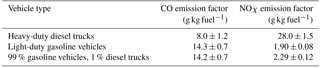
Table 2Reported emission factors of diesel and gasoline vehicles (Dallmann et al., 2011, 2012, 2013). Emissions from medium-duty and heavy-duty diesel trucks, which account for < 1 % of all vehicles, were removed to give the value for light-duty gasoline vehicles.
Here, we propose a model for field calibration that leverages (1) useful cross-sensitivities, (2) chemical conservation equations, (3) knowledge of the global and/or regional background of pollutants, and (4) assumptions based on well-known characteristics of urban air quality and local emissions. The result is a calibration procedure for the drift and temperature dependencies of the 10 calibration parameters that does not require co-location with a reference instrument or prior laboratory experiments for each sensor. The first constraint we apply is the O3 sensors' cross-sensitivity to NO2. Laboratory measurements indicate that this cross-sensitivity is 100 % and we fix it at that value.
Table 3Mean absolute error of comparison between regional O3 and hourly averaged BEACO2N O3 measurements derived from multiple linear regression models of increasing complexity between February and April 2016.
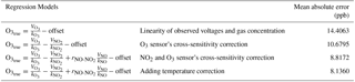
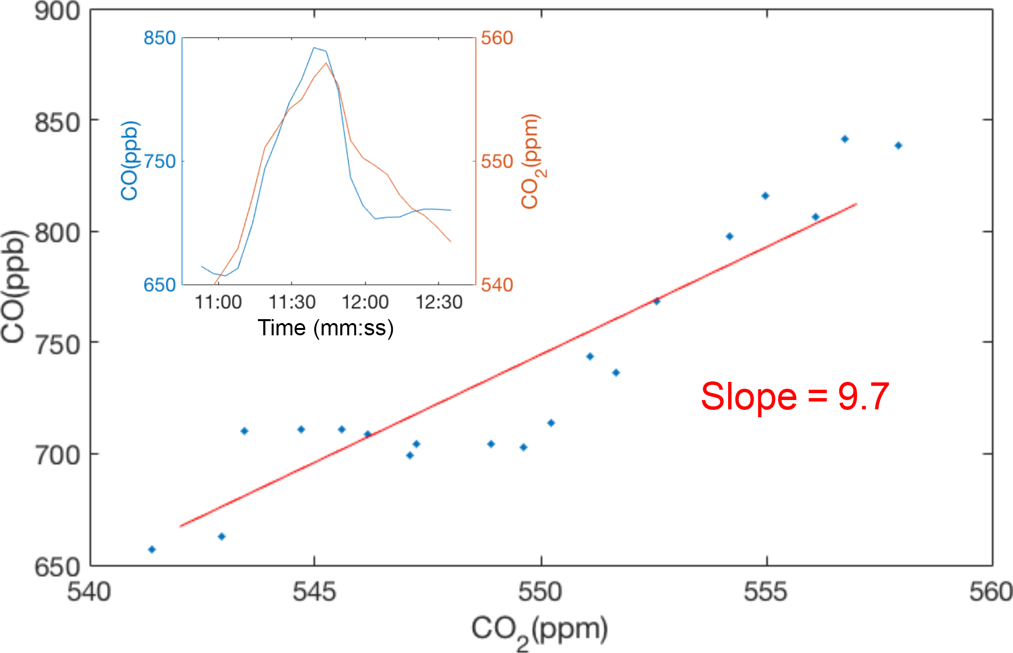
Figure 4Example of CO plume identification and regression against CO2 to find the CO emission factor using raw, 10 s data. The derived CO emission ratio (CO ∕ CO2) for this example is 9.7 ppb ppm−1.
3.1 Regional ozone uniformity to calibrate the NO2 and O3 sensors' sensitivities
The NO, NO2, and O3 sensitivity can be derived from observations with higher-quality instruments at nearby locations. Ozone is a secondary pollutant with small local-scale variation, except in the very near field of NO emissions. The Bay Area Air Quality Management District (BAAQMD) maintains four TECO model 49i ozone analyzers within the BEACO2N study area (see Fig. 1). We choose the closest site among these four regulatory monitoring sites to provide O as a constraint for multiple linear regression of Eq. (5) (derived from Eqs. 2–4). Different BEACO2N nodes are thus referenced to different reference instruments.
Here, offset is a combination of the zero offsets of the NO, NO2, and O3 sensors, all of which can be constrained as detailed in Sect. 3.2 below. The sensitivity of the O3 and NO2 sensors ( and and relationship between the NO-NO2 cross-sensitivity and the sensitivity of the NO sensor ( or ) are obtained by multiple linear regression of Eq. (5).
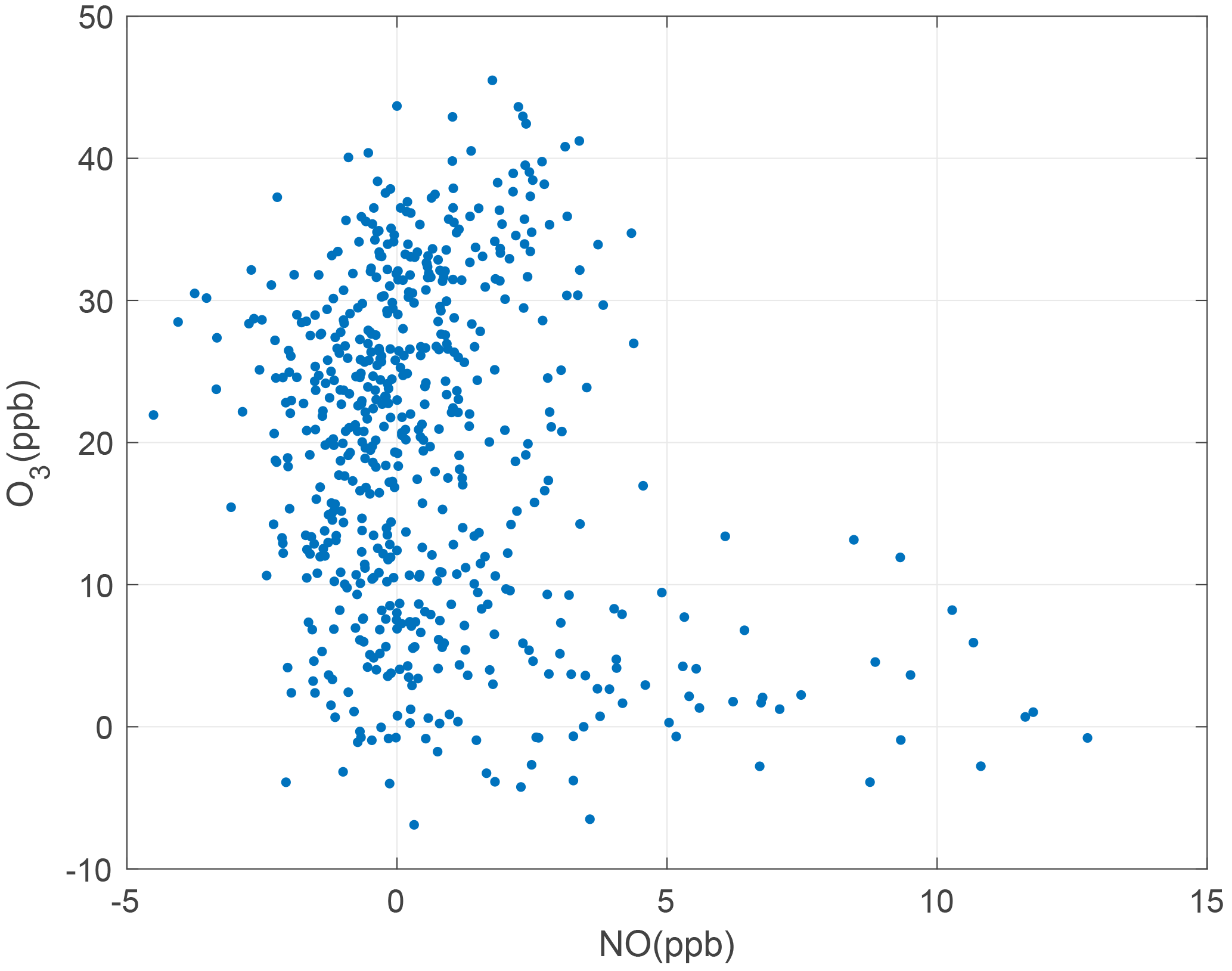
Figure 5Representative month of 1 min averaged NO and O3 measurements taken between 00:00 and 03:00; plumes excluded.
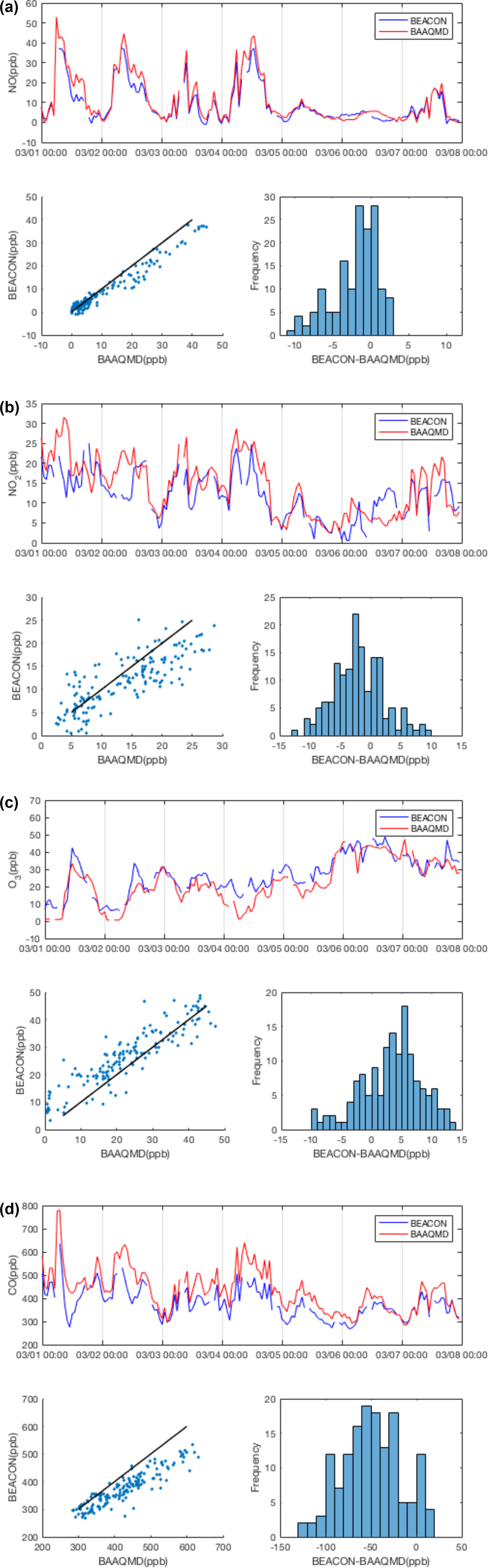
Figure 6Time series (top), direct comparison (bottom left), and histogram (bottom right) of hourly averaged (a) NO, (b) NO2, (c) O3, and (d) CO mixing ratios from a representative week of calibrated BEACO2 N and BAAQMD reference data. The black lines in the bottom left plots indicate the 1:1 line.
3.2 Use of co-emitted gases in plumes to calibrate the CO and NO sensors' sensitivity
The CO and NO sensor cannot be constrained by cross-sensitivity to the other gases. Instead, we constrain the sensitivity by insisting that the median emission factor of CO (or NO) per unit CO2 corresponds to median values reported for the U.S. vehicle fleet. We express the emission factor (EFX, ppb ppm−1) of gas X, which is CO or NO, as in Eq. (6):
Our measurements of the concentration of CO2 are described in Shusterman et al. (2016) and values for EFCO and EF are reported in (Dallmann et al., 2013; see Table 2). We constrain the sensitivity of the CO and NO sensors in the network such that the median ΔX∕ΔCO2 of the plumes is equal to emission factors characteristic of the average vehicle fleet. The NO sensors' sensitivity is constrained by the emission factor of NOX, estimating the upper limit of NO concentration.
Figure 4 shows an example of a measured plume and the derived ΔCO ∕ ΔCO2 ratio. We identify plumes as the local maximum found in a 10 min moving window, starting and ending at the local minima. Each plume is a few minutes in duration, representing an emission ratio averaged over several vehicles. Since diesel trucks have an order of magnitude higher NOX emission factors compared to gasoline vehicles, the percentage of truck traffic near each site affects the median emission factors. The median freeway truck ratio varies little across the BEACO2N network; however, regions with a larger range of median truck ratios will have larger uncertainties or require a calibration approach that accounts for this variation.
3.3 Use of chemical conservation equations near emissions to calibrate the NO, NO2, and O3 sensors' zero offsets
We are able to constrain the zero offsets of NO, NO2 and O3 sensors by taking advantage of proximity to local emission sources and the following chemical conservation equations.
These three reactions result in a steady-state relationship among the nitrogen oxides (NO and ozone. At nighttime, Reaction (R2) does not occur due to the absence of sunlight. In the absence of emissions, the NO concentration goes to zero on nights with sufficient O3. Conversely, near strong emission sources, NO is found in excess of ozone and the O3 concentration goes to zero (see Fig. 5). Using this logic, we identify times between 00:00 to 03:00, when there is zero NO or O3 to define the zero offsets of the NO and O3 sensors, using 1 min averaged data with plumes excluded (see Sect. 3.3 for details of the plume identification procedure).
The NO2 offset can be determined using the pseudo-steady-state (PSS) approximation. We estimate the NO2 concentration through Eq. (7):
Here, (in units of s−1) is the photolysis rate constant for Reaction (R2) and (in units of cm3 molecule−1 s−1) is the rate constant for Reaction (R1). [X] expresses the concentration of gas X in units of molecules cm−3. We use sensitivity corrected (see Sect. 3.1 and 3.2), 1 min average NO and O3 concentrations measured from 12:00 to 15:00, and select data with a time derivative of O3 near zero to ensure that the measurements reflect air that has achieved steady state. The NO2 concentration at PSS is derived using Eq. (7) and the NO2 offset is chosen to ensure the calculated and observed NO2 are equal. NO2 is also produced through the reaction of HO2∕RO2 with NO, but this is omitted from the right-hand side of Eq. (7), resulting in a lower bound of the true NO2 concentration. Estimated NO2 is therefore low by about 5 % in winter and as much as 30 % in summer. If higher accuracy is needed, the reaction of HO2∕RO2 with NO could be considered to reduce this bias.
3.4 Use of global background to calibrate the CO sensors' zero offset
To infer the zero offset of the CO sensor, we follow the procedure outlined in Shusterman et al. (2016) for CO2 sensors. We assume the signal measured at a given site is decomposed as in Eq. (8):
The measurement of the pollutant CO ([CO]ambient) is the sum of regional and local signals ([CO]background and [CO]local, respectively), as well as some offset from the true concentration (offset). Assuming the monthly minimum concentration measured at a given site represents [CO]background, this background signal is compared to that measured at a “supersite” of reference instruments located within the network domain, allowing the offset to be derived. We also assume that when [CO]ambient, as well as [CO]local, is minimum in each day, the concentration measured at a given site has a constant deviation from the background signal. This is a reasonable assumption for the BEACO2N domain as the dominant wind pattern frequently brings unpolluted air from the Pacific Ocean.
3.5 Temperature dependence and temporal drift
In order to account for the temperature and time dependence of calibration parameters, we apply the calibration process described in Sect. 3.1 through 3.4 for temperature increments of 1 ∘C within a 3-month running window. Then, we are able to define a temperature-dependent sensitivity and zero offset, which is used to convert the measured voltages to mixing ratios. In this way, we can also evaluate temporal drift with monthly resolution. The calibration procedure can be repeated for shorter time intervals if wider temperature windows are used.
We evaluate the efficacy of our calibration method using a BEACO2N node co-located with reference instruments at the Laney College monitoring site maintained by the Bay Area Air Quality Management District (BAAQMD). Here we consider data collected from February to April 2016, calibrate them according to the procedure described above (following Sect. 3.1 to 3.5), and compare it against the BAAQMD data. Reference data are collected by a TECO 48i CO analyzer and a TECO 42i NOx analyzer. Ozone data from the “Oakland West” location, the closest ozone-monitoring site maintained by BAAQMD, were used for multiple linear regression of Eq. (5). The zero offset for CO was calculated using BAAQMD data from the Bodega Bay background site (see Fig. 1; Guha et al., 2016) as local “supersite” data were unavailable during this period. A background site closer to the network would likely improve our ability to constrain the CO zero offset; a reference instrument for that purpose was installed in summer 2017.
In our calibration procedure, the cross-sensitivities and temperature dependence are corrected for better accuracy. Table 3 shows the reduction in mean absolute error (MAE) that results when cross-sensitivity and temperature dependence issues are considered during multiple linear regression of Eq. (5). Here, MAE is calculated after conducting the sensitivity correction explained in Sect. 3.1, but before the offset correction in Sect. 3.3. Fully calibrated, hourly averaged BEACO2N sensor data are compared to reference data in Fig. 6. For NO, NO2, O3, and CO the mixing ratio measured agrees reasonably well with the reference instrument with correlation coefficients of 0.88, 0.61, 0.69, and 0.74 and MAE of 3.63, 4.12, 5.04, and 54.93 ppb, respectively. The noise (±2σ) in the differences between the calibrated hourly BEACO2N data and reference data is 9.74 ppb for NO, 9.97 ppb for NO2, 13.04 ppb for O3, and 116.23 ppb for CO. These noise values are dominated by the Alphasense noise except in the case of CO, where noise is evenly split between the low-cost electrochemical sensors and the reference instruments.
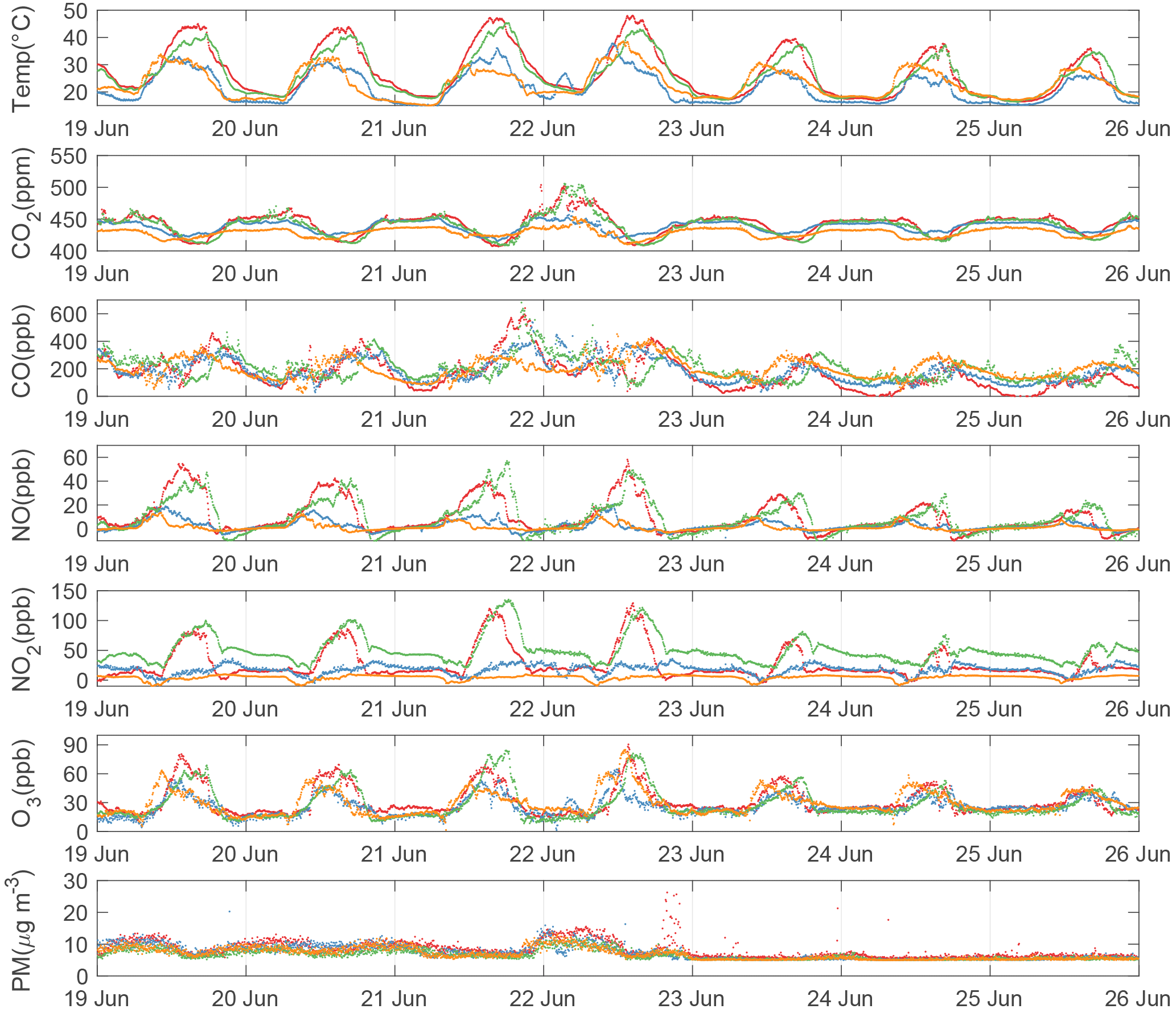
Figure 7Time series of fully calibrated 5 min averaged BEACO2N data from a representative week at four sites deployed in 2017. Observations from the Hercules, Ohlone, Washington, and Madera sites are plotted in red, green, orange, and blue, respectively. Particulate matter is converted to units of mass concentration according to Holstius et al. (2014).
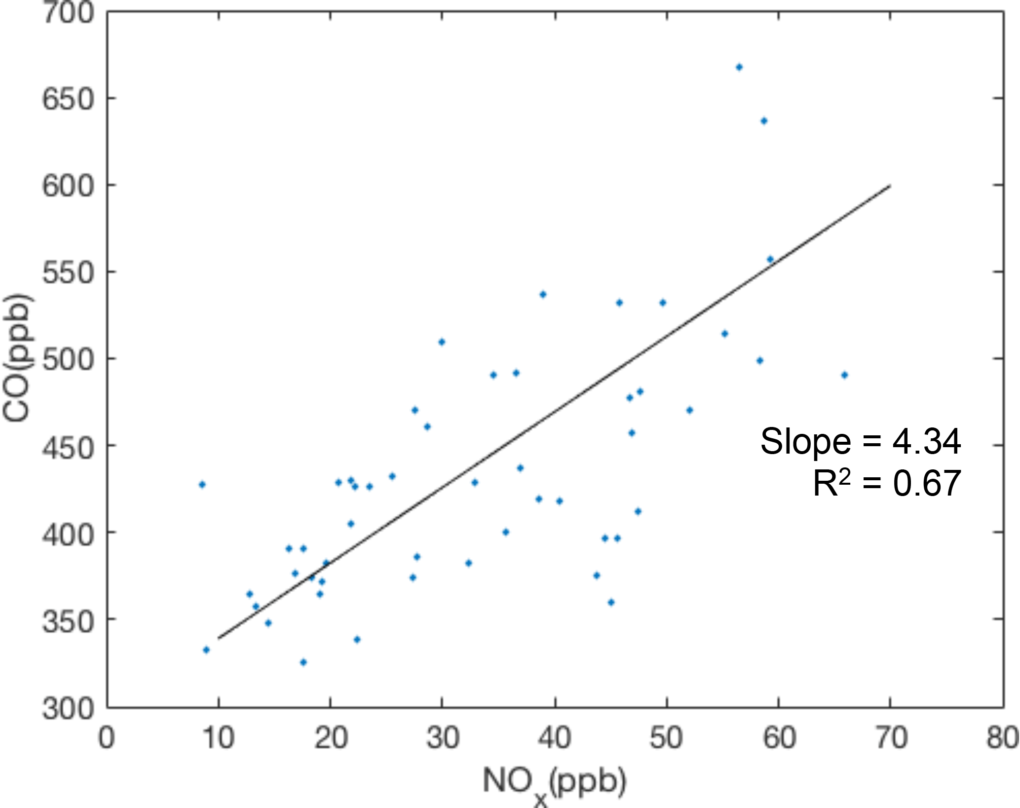
Figure 7 shows a week-long time series of fully calibrated air quality data from four BEACO2N sites in 2017 (see Fig. 1). BEACO2N nodes capture the short-term variability associated with local emissions, superimposed on the diurnal variation caused by mixing and changes in the height of the boundary layer. Large mixing ratios of NO, NO2, and O3 are observed at the Hercules and Ohlone sites, likely representing strong NOx emissions from an oil refinery nearby. The spatial variability of trace gases observed at these four BEACO2N sites provides a more diverse perspective on emissions compared to that provided by the one regulatory monitoring site in the vicinity.
The emission ratios of CO and NOx were also investigated using the BEACO2N data from sample locations. Figure 8 shows ratios observed at the Laney College site. The slope of CO ∕ NOx varies from 4.43 to 12.99 across five BEACO2N sites, reflecting spatial variations in local sources. Sites near roads with more diesel vehicles, such as Laney College, show lower CO ∕ NOx ratios, as expected given diesel vehicles' higher NOx emissions. The range of observed CO ∕ NOx emission ratios is similar to the values reported by McDonald et al. (2013).
Calibration of low-cost sensors is necessary for quantitative analysis. In this paper, we have described a truly low cost, routine in-field calibration method and the evaluation of a fully calibrated low-cost, high-density air quality sensor network. The Alphasense B4 electrochemical gas sensors are able to detect typical diurnal cycles in gas concentrations as well as short-term changes corresponding to chemical reactions and local emissions. These capabilities of the sensors are utilized for a field calibration protocol that does not require co-location with reference instrumentation, but does require reference instruments to be sited within the network domain. The calibrated dataset demonstrates the accuracy required to resolve information relevant to urban emission sources, such as CO ∕ NOx emission ratios. Through this work, we can realize the promise of low-cost, high-density sensor networks as a viable approach for atmospheric monitoring.
The data used in this study can be obtained from the authors upon request.
The authors declare that they have no conflict of interest.
This work was funded by the Bay Area Air Quality Management District
(2016.041), the Health Effects Institute (R-82811201), and the Koret
Foundation. Additional support was provided by a Kwanjeong Educational
Fellowship to Jinsol Kim, an NSF Graduate Research Fellowship to Alexis A. Shusterman, and a Hellman Family Graduate Fellowship to Kaitlyn J. Lieschke.
We acknowledge the use of data sets maintained by BAAQMD's Ambient Air
Monitoring Network, as well as David M. Holstius, Holly L. Maness, and
Virginia Teige for their contributions to BEACO2N's code base.
Edited by: Thomas F. Hanisco
Reviewed by: two anonymous referees
Bart, M., Williams, D. E., Ainslie, B., Mckendry, I., Salmond, J., Grange, S. K., Alavi-Shoshtari, M., Steyn, D., and Henshaw, G. S.: High Density Ozone Monitoring Using Gas Sensitive Semi-Conductor Sensors in the Lower Fraser Valley, British Columbia, Environ. Sci. Technol., 48, 3970–3977, 2014.
Borrego, C., Costa, A. M., Ginja, J., Amorim, M., Coutinho, M., Karatzas, K., Sioumis, T., Katsifarakis, N., Konstantinidis, K., De Vito, S., Esposito, E., Smith, P., Andre, N., Gerard, P., Francis, L. A., Castell, N., Schneider, P., Viana, M., Minguillon, M. C., Reimringer, W., Otjes, R. P., Von Sicard, O., Pohle, R., Elen, B., Suriano, D., Pfister, V., Prato, M., Dipinto, S., and Penza, M.: Assessment of air quality microsensors versus reference methods?: The EuNetAir joint exercise, Atmos. Environ., 147, 246–263, https://doi.org/10.1016/j.atmosenv.2016.09.050, 2016.
Cox, R. M.: The use of passive sampling to monitor forest exposure to O3, NO2 and SO2: a review and some case studies, Environ. Pollut., 126, 301–311, https://doi.org/10.1016/S0269-7491(03)00243-4, 2003.
Cross, E. S., Williams, L. R., Lewis, D. K., Magoon, G. R., Onasch, T. B., Kaminsky, M. L., Worsnop, D. R., and Jayne, J. T.: Use of electrochemical sensors for measurement of air pollution: correcting interference response and validating measurements, Atmos. Meas. Tech., 10, 3575–3588, https://doi.org/10.5194/amt-10-3575-2017, 2017.
Dallmann, T. R., Harley, R. A., and Kirchstetter, T. W.: Effects of Diesel Particle Filter Retrofits and Accelerated Fleet Turnover on Drayage Truck Emissions at the Port of Oakland, Environ. Sci. Technol., 10773–10779, 2011.
Dallmann, T. R., Demartini, S. J., Kirchstetter, T. W., Herndon, S. C., Onasch, T. B., Wood, E. C., and Harley, R. A.: On-Road Measurement of Gas and Particle Phase Pollutant Emission Factors for Individual Heavy-Duty Diesel Trucks, Environ. Sci. Technol., 46, 8511–8518, 2012.
Dallmann, T. R., Kirchstetter, T. W., Demartini, S. J., and Harley, R. A.: Quantifying On-Road Emissions from Gasoline-Powered Motor Vehicles: Accounting for the Presence of Medium- and Heavy-Duty Diesel Trucks, Environ. Sci. Technol., 47, 13873–13881, 2013.
Guha, A., Bower, J., Martien, P., and Perkins, I.: Timeseries of atmospheric dry air mole fractions from continuous measurements at fixed-site GHG monitoring stations in the San Francisco Bay Area, California, 2016.
Hagan, D. H., Isaacman-VanWertz, G., Franklin, J. P., Wallace, L. M. M., Kocar, B. D., Heald, C. L., and Kroll, J. H.: Calibration and assessment of electrochemical air quality sensors by co-location with regulatory-grade instruments, Atmos. Meas. Tech., 11, 315–328, https://doi.org/10.5194/amt-11-315-2018, 2018.
Holstius, D. M., Pillarisetti, A., Smith, K. R., and Seto, E.: Field calibrations of a low-cost aerosol sensor at a regulatory monitoring site in California, Atmos. Meas. Tech., 7, 1121–1131, https://doi.org/10.5194/amt-7-1121-2014, 2014.
Jerrett, M., Donaire-gonzalez, D., Popoola, O., Jones, R., Cohen, R. C., Almanza, E., Nazelle A., Mead, I., Carrasco-Turigas, G., Cole-Hunter, T., Triguero-Mas, M., Seto, E., and Nieuwenhuijsen, M.: Validating novel air pollution sensors to improve exposure estimates for epidemiological analyses and citizen science, Environ. Res., 158, 286–294, https://doi.org/10.1016/j.envres.2017.04.023, 2017.
Jiao, W., Hagler, G., Williams, R., Sharpe, R., Brown, R., Garver, D., Judge, R., Caudill, M., Rickard, J., Davis, M., Weinstock, L., Zimmer-Dauphinee, S., and Buckley, K.: Community Air Sensor Network (CAIRSENSE) project: evaluation of low-cost sensor performance in a suburban environment in the southeastern United States, Atmos. Meas. Tech., 9, 5281–5292, https://doi.org/10.5194/amt-9-5281-2016, 2016.
Krupa, S. V. and Legge, A. H.: Passive sampling of ambient, gaseous air pollutants?: an assessment from an ecological perspective, Environ. Pollut., 107, 31–45, 2000.
Lateb, M., Meroney, R. N., Yataghene, M., Fellouah, H., Saleh, F., and Boufadel, M. C.: On the use of numerical modelling for near-field pollutant dispersion in urban environments. A review, Environ. Pollut., 208, 271–283, https://doi.org/10.1016/j.envpol.2015.07.039, 2016.
Masson, N., Piedrahita, R., and Hannigan, M.: Chemical Approach for quantification of metal oxide type semiconductor gas sensors used for ambient air quality monitoring, Sensor. Actuat. B-Chem., 208, 339–345, https://doi.org/10.1016/j.snb.2014.11.032, 2015.
McDonald, B. C., Gentner, D. R., Goldstein, A. H., and Harley, R. A.: Long-Term Trends in Motor Vehicle Emissions in U.S. Urban Areas, Environ. Sci. Technol., 47, 10022–10031, https://doi.org/10.1021/es401034z, 2013.
Mead, M. I., Popoola, O. A. M., Stewart, G. B., Landshoff, P., Calleja, M., Hayes, M., Baldovi, J. J., McLeod, M. W., Hodgson, T. F., Dicks, J., Lewis, A., Cohen, J., Baron, R., Saffell, J. R., and Jones, R. L.: The use of electrochemical sensors for monitoring urban air quality in low-cost, high-density networks, Atmos. Environ., 70, 186–203, https://doi.org/10.1016/j.atmosenv.2012.11.060, 2013.
Mijling, B., Jiang, Q., de Jonge, D., and Bocconi, S.: Field calibration of electrochemical NO2 sensors in a citizen science context, Atmos. Meas. Tech., 11, 1297–1312, https://doi.org/10.5194/amt-11-1297-2018, 2018.
Moltchanov, S., Levy, I., Etzion, Y., Lerner, U., Broday, D. M., and Fishbain, B.: On the feasibility of measuring urban air pollution by wireless distributed sensor networks, Sci. Total Environ., 502, 537–547, https://doi.org/10.1016/j.scitotenv.2014.09.059, 2015.
Mueller, M., Meyer, J., and Hueglin, C.: Design of an ozone and nitrogen dioxide sensor unit and its long-term operation within a sensor network in the city of Zurich, Atmos. Meas. Tech., 10, 3783–3799, https://doi.org/10.5194/amt-10-3783-2017, 2017.
Papapostolou, V., Zhang, H., Feenstra, B. J., and Polidori, A.: Development of an environmental chamber for evaluating the performance of low-cost air quality sensors under controlled conditions, Atmos. Environ., 171, 82–90, https://doi.org/10.1016/j.atmosenv.2017.10.003, 2017.
Piedrahita, R., Xiang, Y., Masson, N., Ortega, J., Collier, A., Jiang, Y., Li, K., Dick, R. P., Lv, Q., Hannigan, M., and Shang, L.: The next generation of low-cost personal air quality sensors for quantitative exposure monitoring, Atmos. Meas. Tech., 7, 3325–3336, https://doi.org/10.5194/amt-7-3325-2014, 2014.
Sadighi, K., Coffey, E., Polidori, A., Feenstra, B., Lv, Q., Henze, D. K., and Hannigan, M.: Intra-urban spatial variability of surface ozone and carbon dioxide in Riverside, CA: viability and validation of low-cost sensors, Atmos. Meas. Tech. Discuss., https://doi.org/10.5194/amt-2017-183, in review, 2017.
Shusterman, A. A., Teige, V. E., Turner, A. J., Newman, C., Kim, J., and Cohen, R. C.: The BErkeley Atmospheric CO2 Observation Network: initial evaluation, Atmos. Chem. Phys., 16, 13449–13463, https://doi.org/10.5194/acp-16-13449-2016, 2016.
Spinelle, L., Gerboles, M., Gabriella, M., and Aleixandre, M.: Field calibration of a cluster of low-cost available sensors for air quality monitoring. Part A: Ozone and nitrogen dioxide, Sensor. Actuat. B-Chem., 215, 249–257, https://doi.org/10.1016/j.snb.2015.03.031, 2015.
Spinelle, L., Gerboles, M., Gabriella, M., and Aleixandre, M.: Field calibration of a cluster of low-cost commercially available sensors for air quality monitoring. Part B: NO, CO and CO2, Sensor. Actuat. B-Chem., 238, 706–715, https://doi.org/10.1016/j.snb.2016.07.036, 2017.
Sun, L., Wong, K. C., Wei, P., Ye, S., Huang, H., and Yang, F.: Development and Application of a Next Generation Air Sensor Network for the Hong Kong Marathon 2015 Air Quality Monitoring, Sensors, 16, 211, https://doi.org/10.3390/s16020211, 2015.
Vardoulakis, S., Fisher, B. E. A., Pericleous, K., and Gonzalez-flesca, N.: Modelling air quality in street canyons?: a review, Atmos. Environ., 37, 155–182, 2003.
Williams, D. E., Henshaw, G. S., Bart, M., Laing, G., Wagner, J., Naisbitt, S., and Salmond, J. A.: Validation of low-cost ozone measurement instruments suitable for use in an air-quality monitoring network, Meas. Sci. Technol., 24, 065803, https://doi.org/10.1088/0957-0233/24/6/065803, 2013.
Zimmerman, N., Presto, A. A., Kumar, S. P. N., Gu, J., Hauryliuk, A., Robinson, E. S., Robinson, A. L., and R. Subramanian: A machine learning calibration model using random forests to improve sensor performance for lower-cost air quality monitoring, Atmos. Meas. Tech., 11, 291–313, https://doi.org/10.5194/amt-11-291-2018, 2018.