the Creative Commons Attribution 3.0 License.
the Creative Commons Attribution 3.0 License.
Improved model for correcting the ionospheric impact on bending angle in radio occultation measurements
Sean Elvidge
Sean B. Healy
The standard approach to remove the effects of the ionosphere from neutral atmosphere GPS radio occultation measurements is to estimate a corrected bending angle from a combination of the L1 and L2 bending angles. This approach is known to result in systematic errors and an extension has been proposed to the standard ionospheric correction that is dependent on the squared L1 ∕ L2 bending angle difference and a scaling term (κ). The variation of κ with height, time, season, location and solar activity (i.e. the F10.7 flux) has been investigated by applying a 1-D bending angle operator to electron density profiles provided by a monthly median ionospheric climatology model. As expected, the residual bending angle is well correlated (negatively) with the vertical total electron content (TEC). κ is more strongly dependent on the solar zenith angle, indicating that the TEC-dependent component of the residual error is effectively modelled by the squared L1 ∕ L2 bending angle difference term in the correction. The residual error from the ionospheric correction is likely to be a major contributor to the overall error budget of neutral atmosphere retrievals between 40 and 80 km. Over this height range κ is approximately linear with height. A simple κ model has also been developed. It is independent of ionospheric measurements, but incorporates geophysical dependencies (i.e. solar zenith angle, solar flux, altitude). The global mean error (i.e. bias) and the standard deviation of the residual errors are reduced from and for the uncorrected case to rad and rad, respectively, for the corrections using the κ model. Although a fixed scalar κ also reduces bias for the global average, the selected value of κ (14 rad−1) is only appropriate for a small band of locations around the solar terminator. In the daytime, the scalar κ is consistently too high and this results in an overcorrection of the bending angles and a positive bending angle bias. Similarly, in the nighttime, the scalar κ is too low. However, in this case, the bending angles are already small and the impact of the choice of κ is less pronounced.


It has been demonstrated that, by using variational data assimilation techniques, GPS radio occultation (GPS-RO) measurements can be assimilated into operational numerical weather prediction (NWP) systems to improve the accuracy of temperatures in the upper troposphere and lower–middle stratosphere (Healy and Thépaut, 2006; Poli et al., 2009; Rennie, 2010). In particular, GPS-RO measurements reduce stratospheric temperature biases in NWP systems and this indicates that such measurements could have an increasingly important role in climate monitoring and climate reanalyses (Poli et al., 2010; Steiner et al., 2013). Notwithstanding the benefits of GPS-RO for the neutral atmosphere, it remains necessary to consider the effect of the ionosphere on the measurements.
Vorob'ev and Krasil'nikova (1994) (hereafter referred to as VK94) proposed a method of combining the GPS-RO bending angles measured at two frequencies (L1 and L2) to provide a first-order correction for the ionosphere. VK94 also showed that the first-order correction leaves a systematic bending angle bias that increases as a function of the electron density squared, integrated over the vertical profile. The relationship between the bias and electron density suggests that the bending angle biases should vary diurnally and as a function of the 11-year solar cycle. This has been demonstrated by various authors, e.g. Kursinski et al. (1997), Mannucci et al. (2011) and Danzer et al. (2013).
Healy and Culverwell (2015) have proposed a modification to the standard bending angle correction to reduce the residual systematic ionospheric errors. The modification introduces a new second-order term that is a function of the square of L1 and L2 bending angle difference and a weighting term (κ). The aim of this work is to investigate the variation of κ with height, time, season, location and solar activity (i.e. the F10.7 flux). This has been done by applying a 1-D bending angle operator to electron density profiles provided by the NeQuick monthly median ionospheric climatology model (Nava et al., 2008). As well as examining the variations in κ, a κ model has been developed. It is independent of ionospheric measurements and therefore simple to implement in an operational system, but does incorporate the relevant geophysical dependencies (i.e. solar zenith angle, solar flux). The expectation is that, since NeQuick is a reasonable median model of the ionosphere, the κ model derived from it will also exhibit reasonable statistics, though this has not been proven.
Radio occultations, the VK94 ionospheric correction procedure and the proposed modified correction are described in Sect. 2. Examples of how κ varies with height, location and solar activity are presented in Sect. 3. Models for κ are proposed and assessed in Sect. 4 and the discussion and conclusions are given in Sects. 5 and 6.
Hardy et al. (1994), Kursinski et al. (1997) and Hajj et al. (2002) provide a comprehensive description of the GPS-RO technique. In summary, the GPS satellites transmit on two L-band channels (L1, L2) at f1=1575.42 MHz and f2=1227.60 MHz and the signals are received by a satellite in low earth orbit (LEO) (Fig. 1).
Table 1Updates to produce the University of Birmingham (UoB) variant of NeQuick.
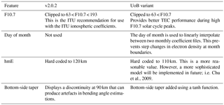
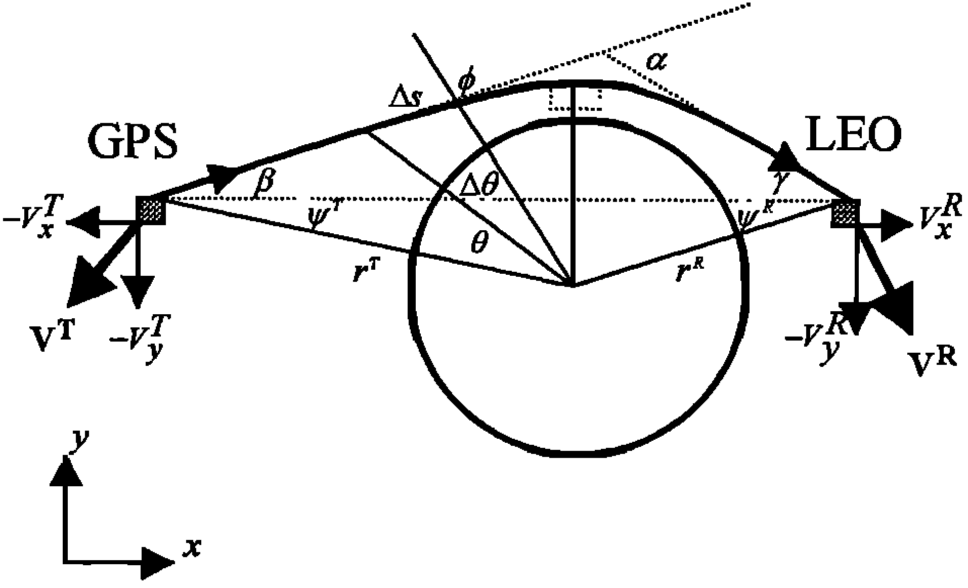
Figure 1Radio occultation geometry. Reproduced from Healy (2001).
The standard approach (Abel transform) for inverting GPS-RO measurements requires the assumption of spherical symmetry. Under that assumption, the bending angle of the ray between the GPS satellite and a receiver in LEO is
where depending on the frequency, a is the impact parameter, rt is the tangent height of the ray path and ni is the refractive index. The impact parameter is given by
Horizontal gradients will result in residual errors in the inversion. However, it is expected that these errors are random; therefore, they should not affect monthly or seasonal climatologies.
To a first-order approximation, the refractive index comprises terms dependent on the neutral atmosphere refractivity (Nn), the ionospheric electron density (ne) and the frequency (f) squared:
where . Therefore, the measured L1 and L2 bending angles are different from each other and contain both neutral and ionospheric components. The standard approach taken in operational RO processing centres is to estimate a corrected neutral atmosphere bending angle (αc) using the VK94 approach:
where the L1 and L2 bending angles (αL1 and αL2 respectively) are interpolated to a common impact parameter. The first-order approximation neglects terms involving higher powers of the frequency and the earth's magnetic field; however, these have little effect on the residual bending angle errors (Syndergaard, 2000). One benefit of this approach is that it is based on the standard parameters estimated by the RO retrieval system and does not require a priori information about the ionosphere. One downside is that a systematic bending angle error remains (see Eq. 5 of Healy and Culverwell, 2015). The bending angle error has a dependence on the electron density squared, which indicates that it will vary with the solar cycle. This has been recognised as a potential source of bias in climatology products (Danzer et al., 2013). Healy and Culverwell (2015) have proposed a modification to the standard ionospheric correction of the following form:
where the κ term compensates for the systematic residual error in the standard approach. An appropriate value for κ has been investigated using simple analytic functions for the ionosphere (Healy and Culverwell, 2015) and using a ray tracer through a 3-D ionospheric model (Danzer et al., 2015), though it should be noted that this study was limited to a low latitude band because of noise in the simulation system. It has been shown that κ generally falls in the range of 10 to 20 rad−1 and a simple scalar model, κ∼14, provides a good first approximation, improving the accuracy of the “dry” temperature retrievals (Danzer et al., 2015). Nevertheless, it is clear that κ will vary as a function of height, local time, season, location and solar activity and therefore it is possible that existing ionospheric climatology models could be used to compute an improved correction term by modelling the monthly mean, temporal and spatial variations of κ more realistically.
A monthly median 3-D ionospheric model (in this case NeQuick) and a 1-D bending angle operator (based on Eq. 1) can be used to estimate the residual ionospheric error and thereby estimate values for κ.
3.1 NeQuick

NeQuick is a monthly median ionospheric electron density model developed at the Aeronomy and Radiopropagation Laboratory (now Telecommunications/ICT for Development Laboratory) of the Abdus Salam International Centre for Theoretical Physics (ICTP), Trieste, Italy, and at the Institute for Geophysics, Astrophysics and Meteorology (IGAM) of the University of Graz, Austria (Nava et al., 2008). The model is based on the Di Giovanni–Radicella (DGR) model (Di Giovanni and Radicella, 1990), which was modified for the European Cooperation in Science and Technology (COST) Action 238 to provide electron densities from ground to 1000 km. The model has been designed to have continuously integrable vertical profiles which allows for rapid calculation of the total electron content (TEC) for transionospheric propagation applications. The current version of NeQuick can be run up to a height of 20 000 km and a variant is used in the Galileo Global Navigation Satellite System (GNSS) to calculate ionospheric corrections (Angrisano et al., 2013).
NeQuick is a “profiler” which makes use of three profile anchor points at the E layer peak, the F1 peak and the F2 peak. To specify the anchor points it uses the layer critical frequencies (foE, foF1, foF2) and the F2 maximum usable frequency factor (M3000(F2)) (Davies, 1965). foE is determined using a solar zenith angle model, foF1 is assumed to be proportional to foE during daytime and zero during nighttime, and foF2 and M3000(F2) are derived from the ITU-R (CCIR) coefficients in the same way as the International Reference Ionosphere (IRI) (Bilitza and Reinisch 2008).
Between 100 km and the peak of the F2 layer, NeQuick uses an electron density profile based on the superposition of five semi-Epstein layers (Epstein, 1930; Rawer, 1983); i.e. the Epstein layers have different thickness parameters for their top and bottom sides. The top side of NeQuick is a simplified approximation to a diffusive equilibrium. A semi-Epstein layer represents the model top side with a height-dependent thickness parameter that has been empirically determined.
The model used in this work is the University of Birmingham's translation of the NeQuick v2.0.2 from FORTRAN into Python. Very minor (negligible) differences in results are observed due to the use of different interpolation routines. The Python code has been largely vectorised to increase the speed of operation. Some additional modifications have been made and are described in Table 1.
3.2 κ estimation
In each of the examples shown in the following sections the same basic procedure has been followed to estimate the value of κ:
-
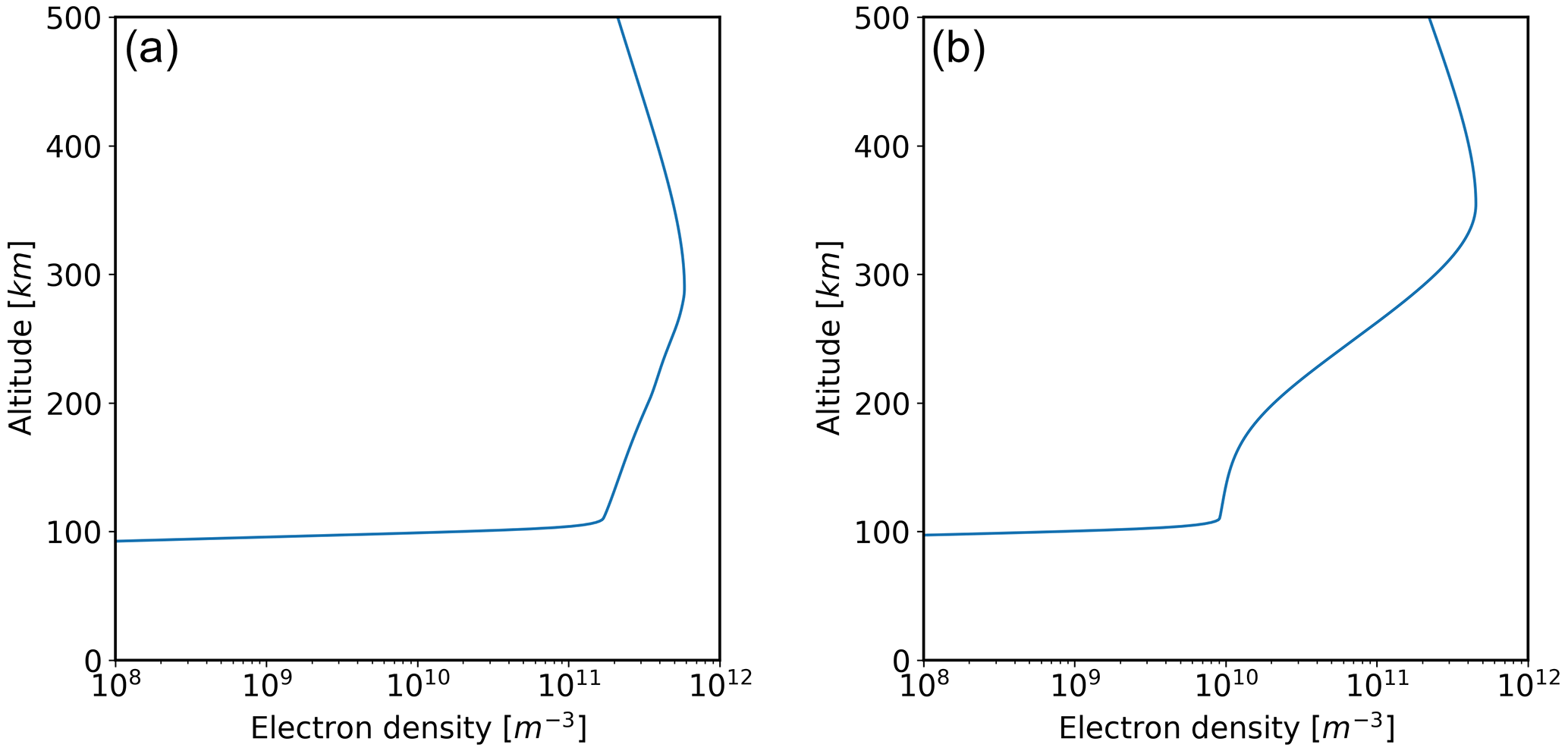
Use NeQuick to estimate a vertical profile of electron density.
-
Convert the electron density (ne) to the refractive index (ni) using the first-order approximation for each frequency (L1 and L2).
-
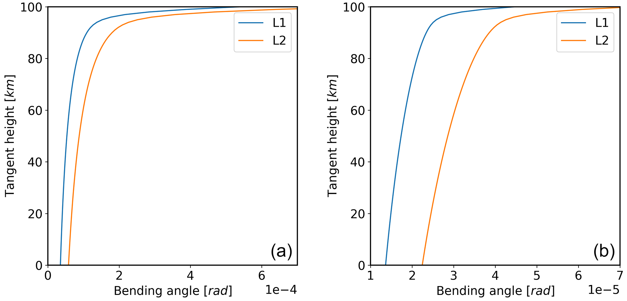
Estimate bending angle using the 1-D observation operator for L1 and L2.
-
Form the VK94 corrected bending angle (αc).
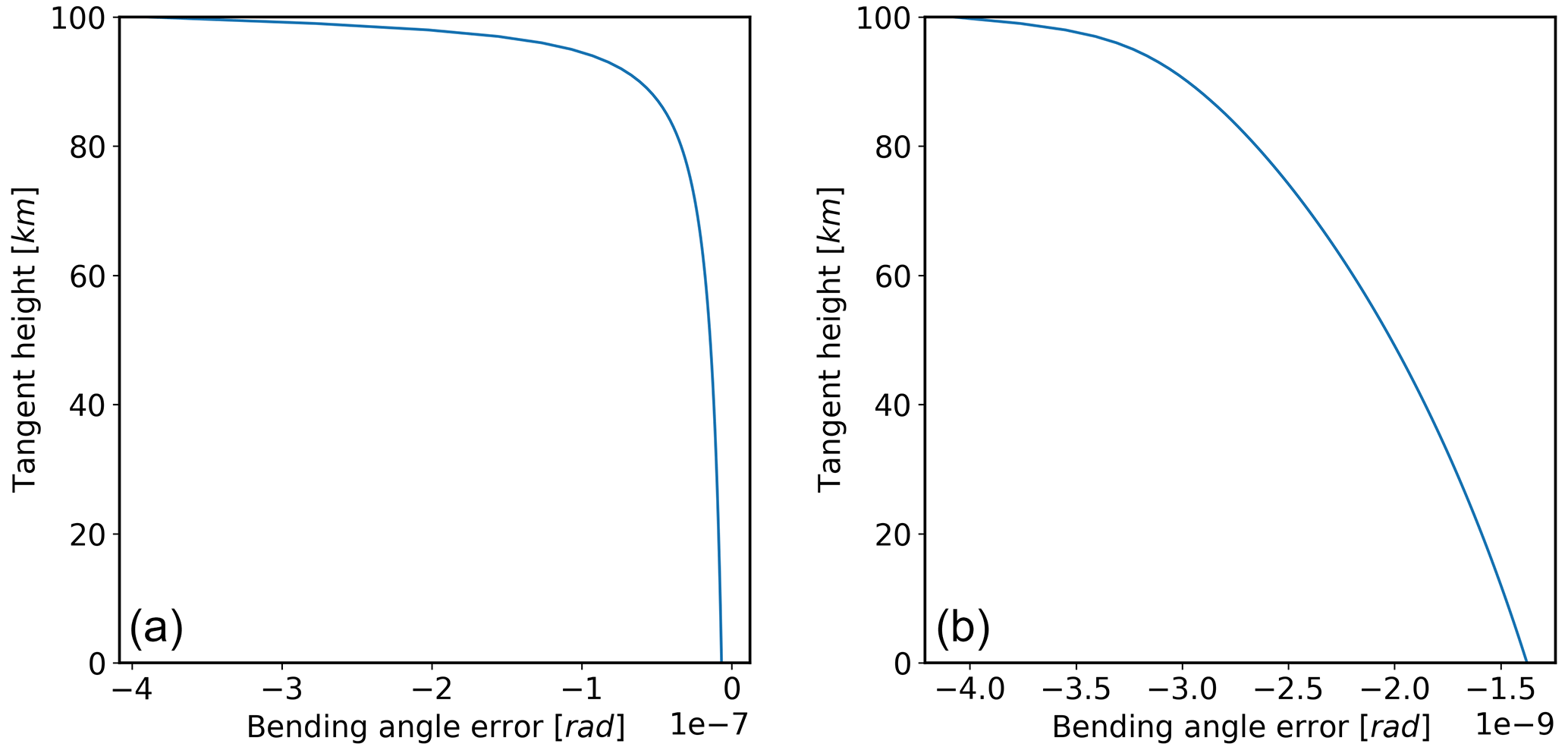
Since no neutral atmosphere is included in the estimate of the refractive index, αc should be zero if VK94 provides a perfect correction. Any non-zero values are representative of the residual ionospheric error (Δα), which, from Eq. (5), is modelled as
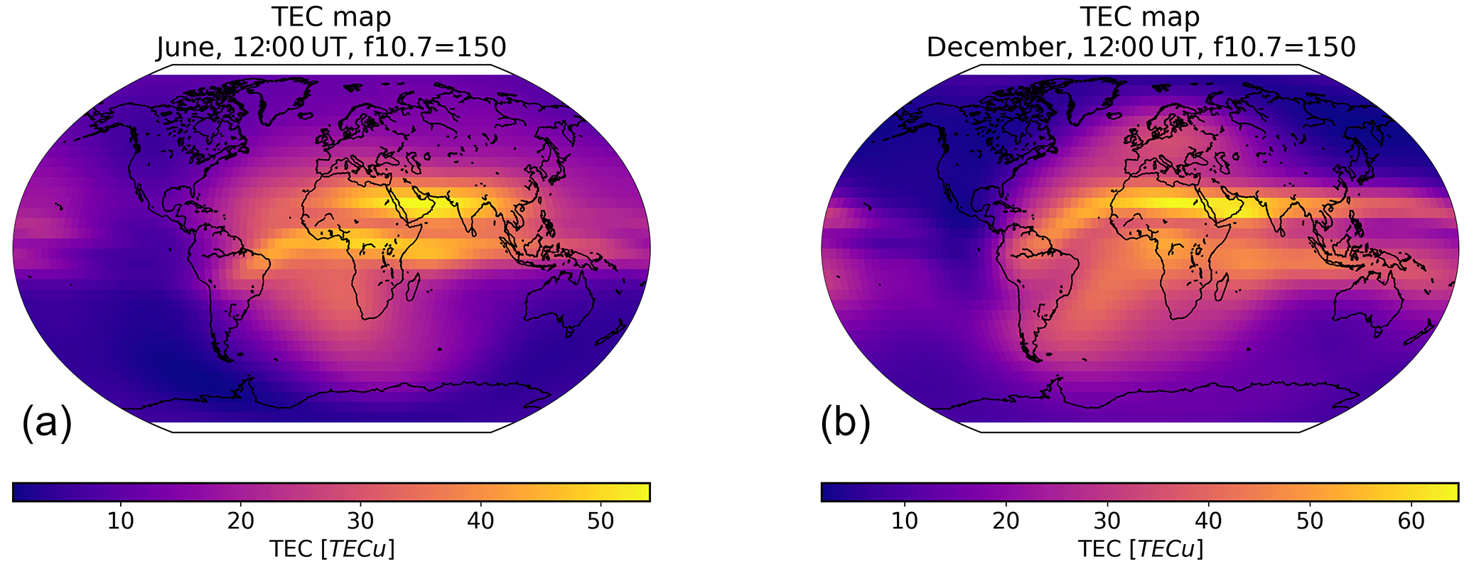
Figure 6Vertical TEC from NeQuick for 12:00 UT, F10.7 = 150: June (a) and December (b). electrons m−2.
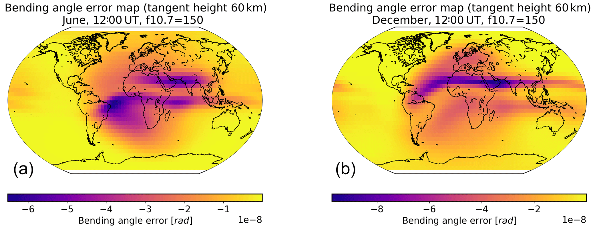
Figure 7Estimated residual bending angle error for 12:00 UT, F10.7 = 150: June (a) and December (b).
Since the bending angles are known, this can be rearranged to provide an estimate of κ as a function of the impact parameter:
In real data the corrected bending angles increase rapidly towards the surface. This means that the impact of any residual error becomes less insignificant below approximately 40 km. Furthermore, the VK94 correction assumes that the ray impact parameter/tangent height is below the ionosphere (i.e. the electron density is zero). Consequently, the main area of interest for κ estimation is between 40 and 80 km. It is in this region where the residual error from the ionospheric correction is likely to be a major contributor to the overall error budget of neutral atmosphere retrievals.
3.3 Height dependence
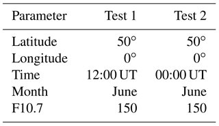
The Figs. 2 to 5 show two examples of the vertical electron density profile, the L1 ∕ L2 bending angles, the residual error and κ. The test parameters are given in Table 2. Over the height range of interest (40–80 km), Fig. 5 shows that κ is approximately linear with tangent height, but its gradient is dependent on the local time.
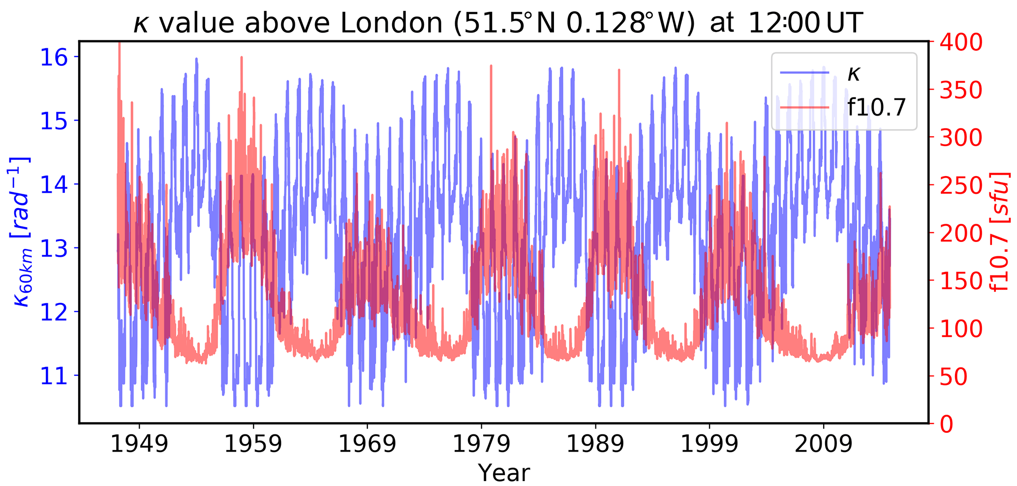
Figure 9Solar cycle dependence of κ for a fixed location (London), tangent height (60 km) and local time (12:00 UT). 1 sfu = 10−22 Wm−2 Hz−1.
3.4 Geographic dependence
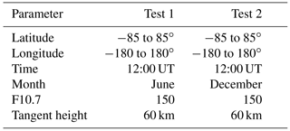
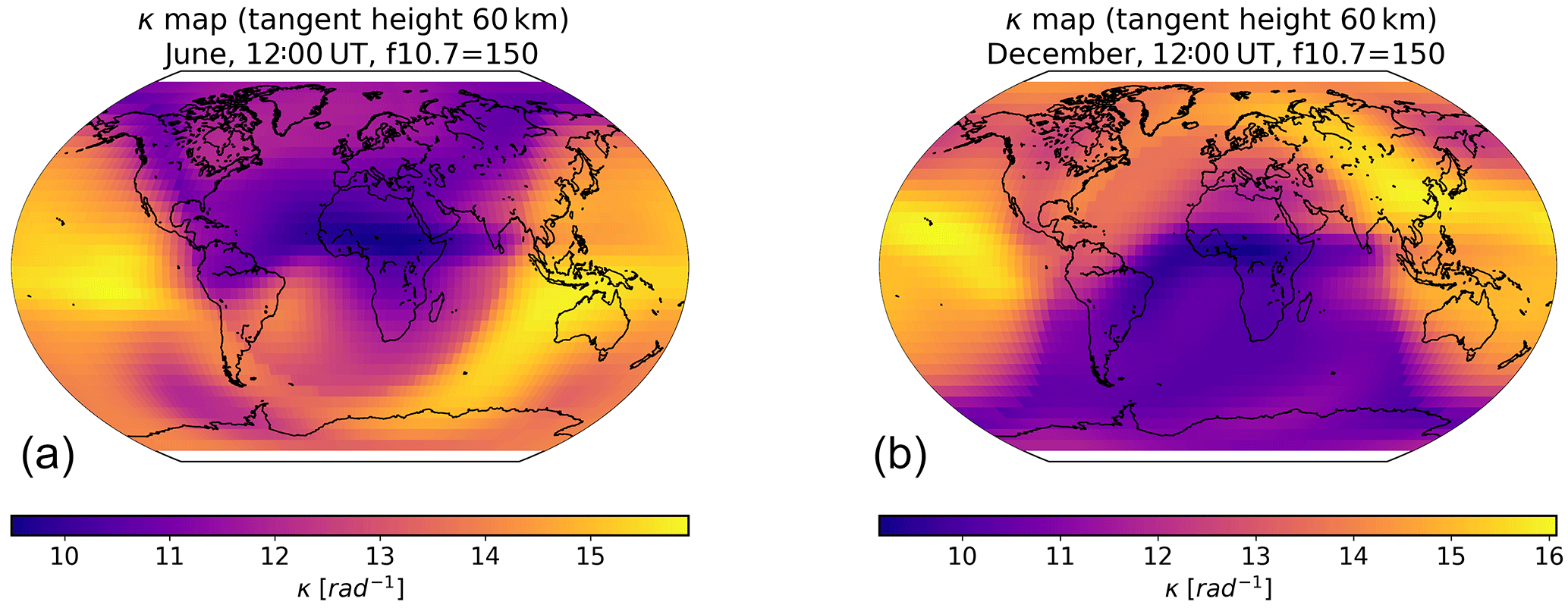
The geographic dependence of bending angle correction can be demonstrated by plotting maps of the TEC (Fig. 6), residual bending angle (Fig. 7) and κ (Fig. 8). In this case, the test parameters are given in Table 3. As expected, the residual bending angle is well correlated (negatively) with the vertical TEC. However, κ is more strongly dependent on the solar zenith angle, indicating that the TEC-dependent component of the residual error is largely modelled by the squared L1 ∕ L2 bending angle difference term in the correction and that κ is modelling other features such as changes in hmF2.
3.5 Solar cycle dependence
The solar cycle dependence of κ has been investigated by estimating κ at a tangent height of 60 km above London for each day over the last 60 years (Table 4). The results (Fig. 9) show that κ is negatively correlated with F10.7; i.e. κ is low when the vertical TEC is large, which occurs when F10.7 is high. Furthermore, the dynamic range of κ is considerably smaller than that of the F10.7 (and hence TEC and bending angle), varying by a factor of approximately 50 % compared to approximately 300 % for F10.7. This, again, is indicative of the TEC-dependent component of the residual error being largely modelled by the squared L1 ∕ L2 bending angle difference term in the correction.
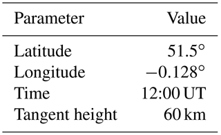
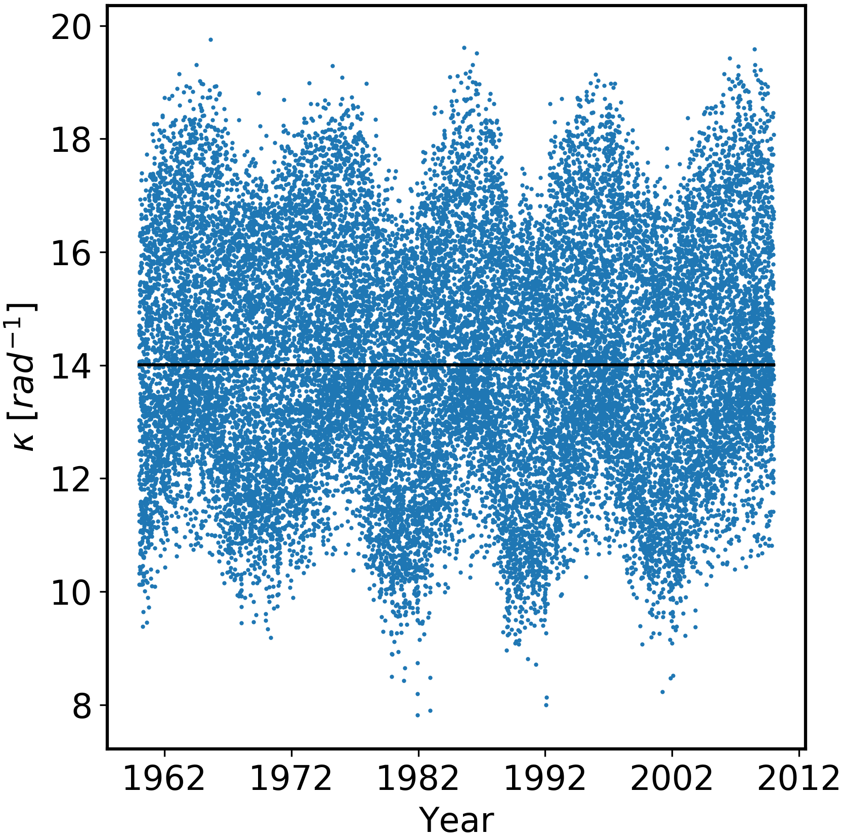
Figure 10κ values for a random set of 25 000 locations and times. The horizontal line marks the median (14 rad−1).
4.1 Introduction
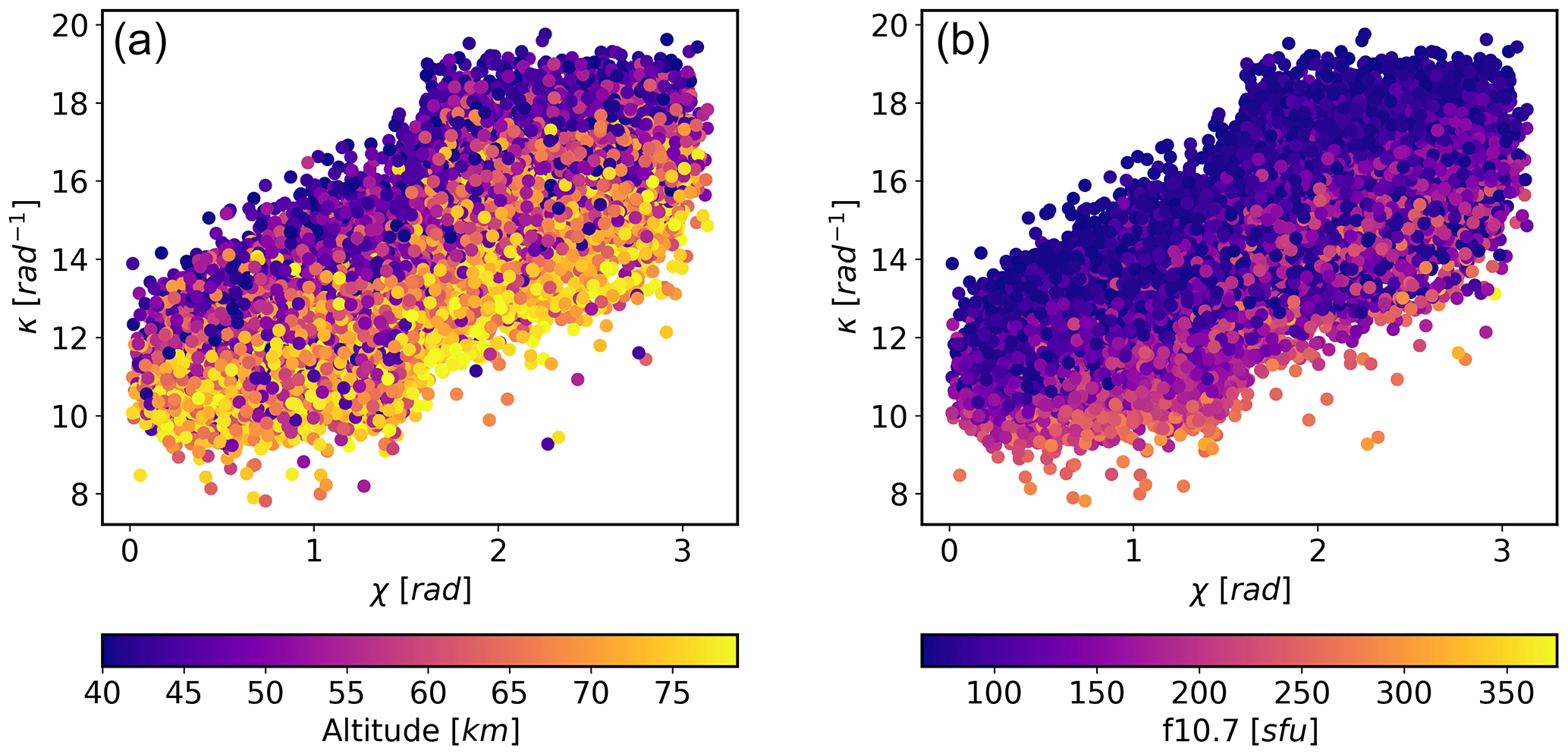
Figure 11κ vs. solar zenith angle (χ), colour coded by altitude (a) and F10.7 (b). 1 sfu = 10−22 Wm−2 Hz−1.
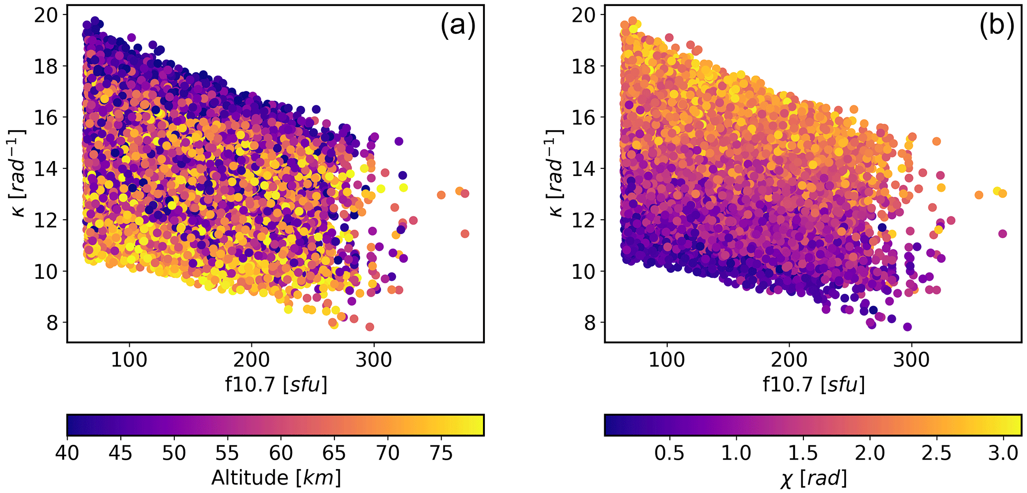
Figure 12κ vs. F10.7, colour coded by altitude (a) and solar zenith angle (χ) (b). 1 sfu = 10−22 Wm−2 Hz−1.

Figure 13κ vs. altitude, colour coded by solar zenith angle (χ) (a) and F10.7 (b). 1 sfu = 10−22 Wm−2 Hz−1.
Section 3 has presented examples of how κ can vary spatially and with solar cycle. In this section, simple models of κ will be assessed in order to evaluate their potential to reduce the residual bending angle errors in the VK94 correction. Three models will be considered:
-
κ equals zero (zero-κ): this represents the current situation with the unmodified VK94 correction.
-
κ is a scalar (scal-κ): this is the approach proposed by Healy and Culverwell (2015).
-
κ is a function of latitude, longitude, solar zenith angle and solar flux (func-κ).
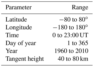
In order to build the models a set of 25 000 κ estimates were generated from NeQuick using random drivers (uniformly distributed over the ranges in Table 5). The true solar flux is used for each randomly selected day and year. A further independent set of 25 000 κ estimates was also generated using the same random parameter ranges to act as a test data set.
4.2 Scalar κ
The random κ values are shown in Fig. 10. The median value is marked by the horizontal line and has value of 14 rad−1. This value is used as the scalar model.
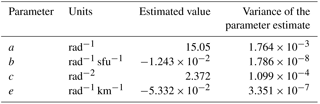
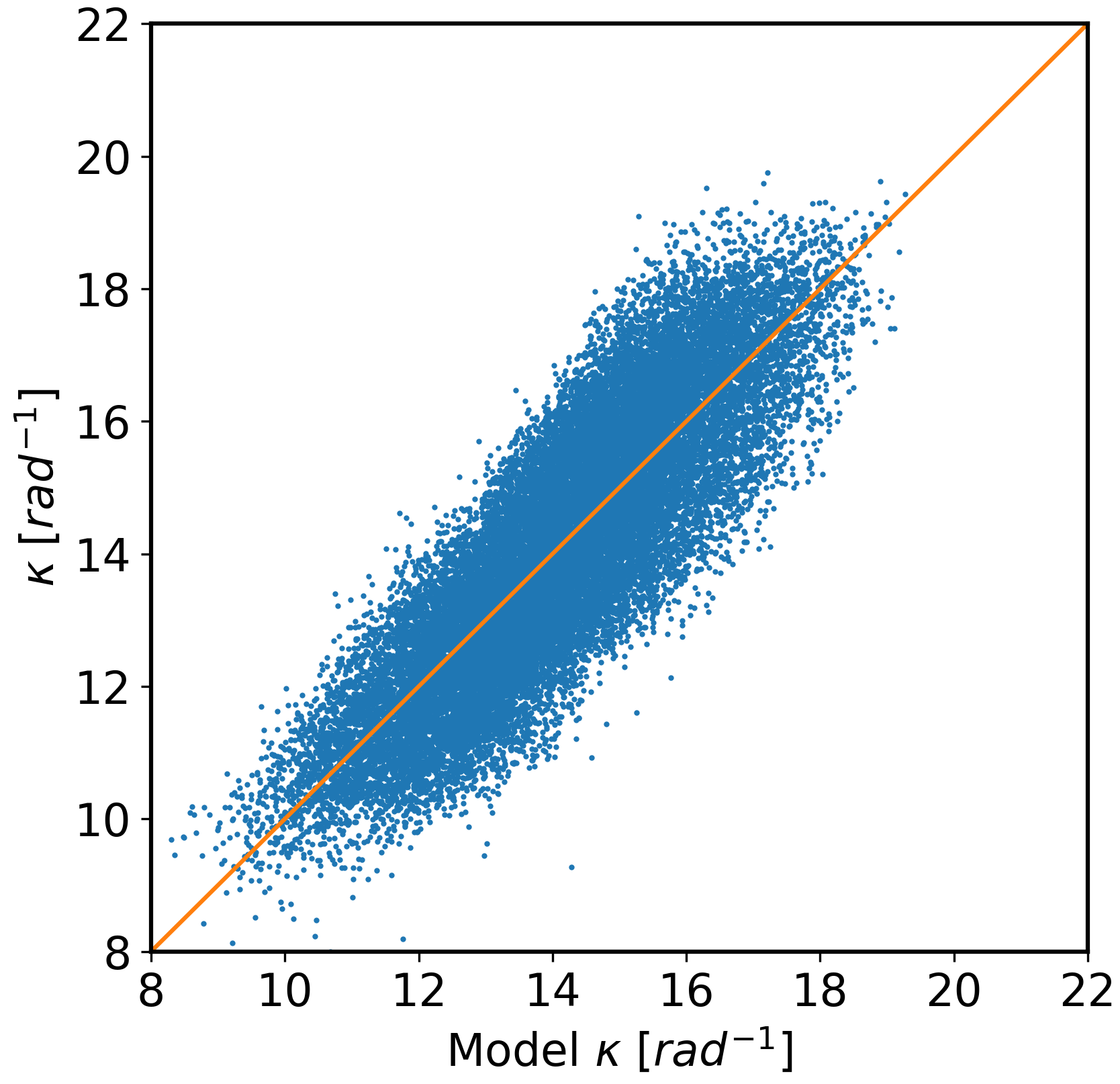
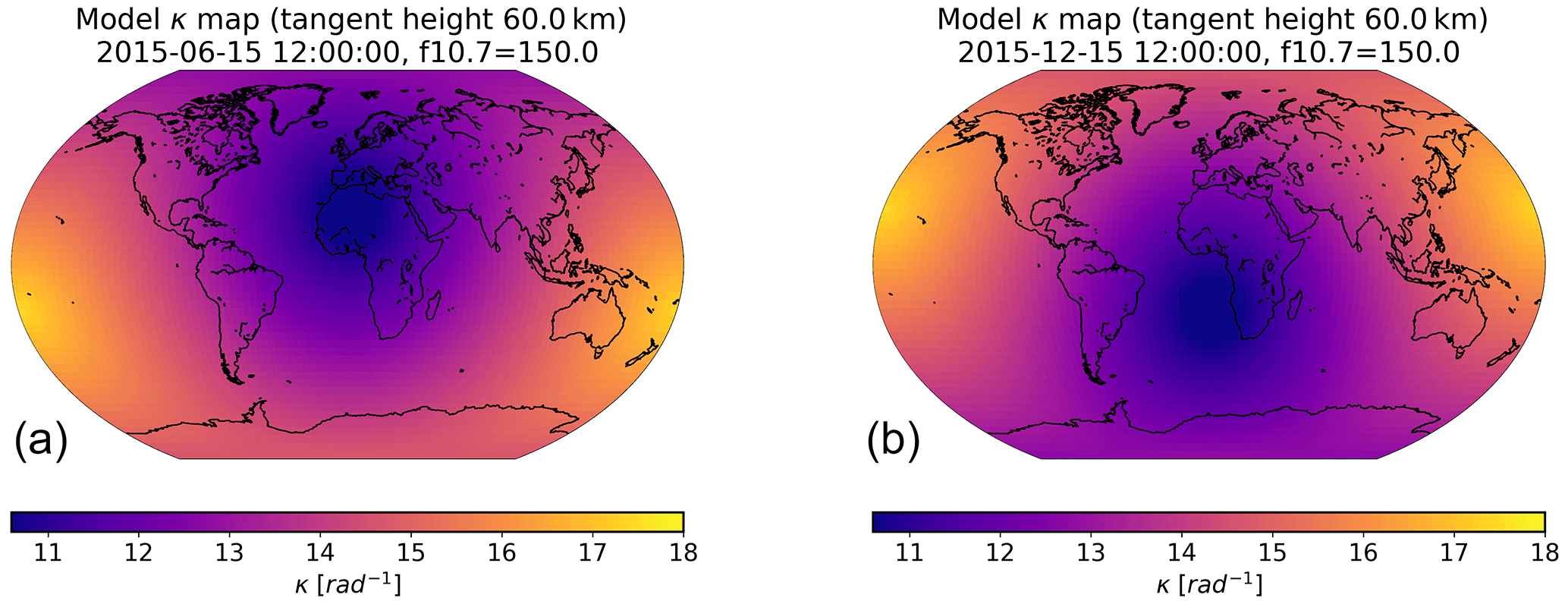
Table 7Global, daytime and nighttime bending angle errors for three models
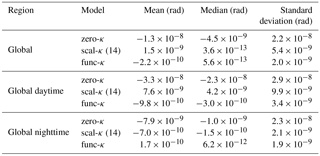
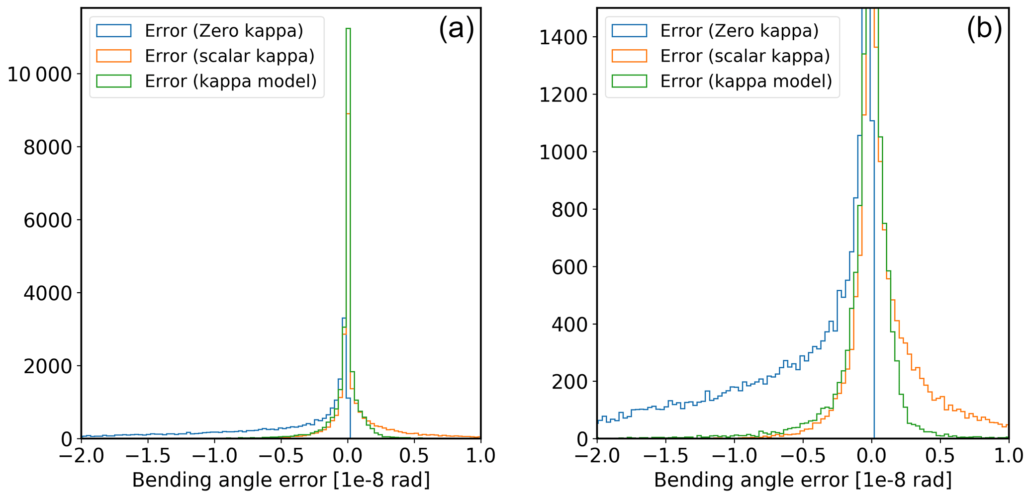
Figure 16Histograms of globally distributed bending angle errors for zero κ, scalar κ and modelled κ. (a) Full histogram. (b) Zoomed to highlight tails.
4.3 Functional form κ
The aim of this model is to produce a very simple polynomial function that mimics some of the form of κ that is not accounted for by the scalar model. Figure 8 is suggestive that κ is a function of solar zenith angle – this is a convenient parameter to use since it embodies the position, local time and season. Figures 11, 12 and 13 show κ as a function of solar zenith angle, F10.7 and altitude respectively. Note that the solar zenith angle has been extended to π radians to account for when the sun is below the horizon. The figures indicate broadly linear dependencies in all cases; therefore, the following model is proposed:
where f10.7 is the F10.7 flux (sfu, 1 sfu = 10−22 Wm−2 Hz−1), χ is the solar zenith angle (rad) and h is the height above the ground (km); and e are scalars to be found by fitting the model to the data.
The Python code curve_fit from the scipy.optimize package has been used to fit the model. The parameter results and the associated variances are shown in Table 6. A plot of the NeQuick estimated κ compared to the func-κ is shown in Fig. 14. Figure 15 shows the geographic distribution of func-κ at 12:00 UT in June and December at 60 km altitude and with an F10.7 of 150. These maps can be directly compared with those in Fig. 8.
4.4 Bending angle error reduction
The second set of 25 000 randomly distributed points has been used to assess the reduction in residual bending angle for each of the κ models (zero-κ, scal-κ and func-κ). Figure 16 shows a histogram of the residual bending angle errors for the full data set. The bending angle error statistics are in Table 7.
Both the scal-κ and func-κ results are an improvement over the zero-κ results. In the case of the scal-κ, both the standard deviation and the mean error (i.e. bias) of the residual bending angle errors are reduced by an order of magnitude compared to the zero-κ results (from and for the zero-κ case to rad and rad respectively; Table 7). In the case of the func-κ, the standard deviation and the mean error (i.e. bias) of the residual bending angle errors are further reduced to rad and rad respectively. Although the scal-κ reduces bias for the global average, the geographic variation of κ (shown in Figs. 8 and 15) makes it clear that the selected value of κ (14 rad−1) is, in fact, only appropriate for a small band of locations around the solar terminator. The effect of this is clear if the residual error statistics are considered for daytime and nighttime separately.
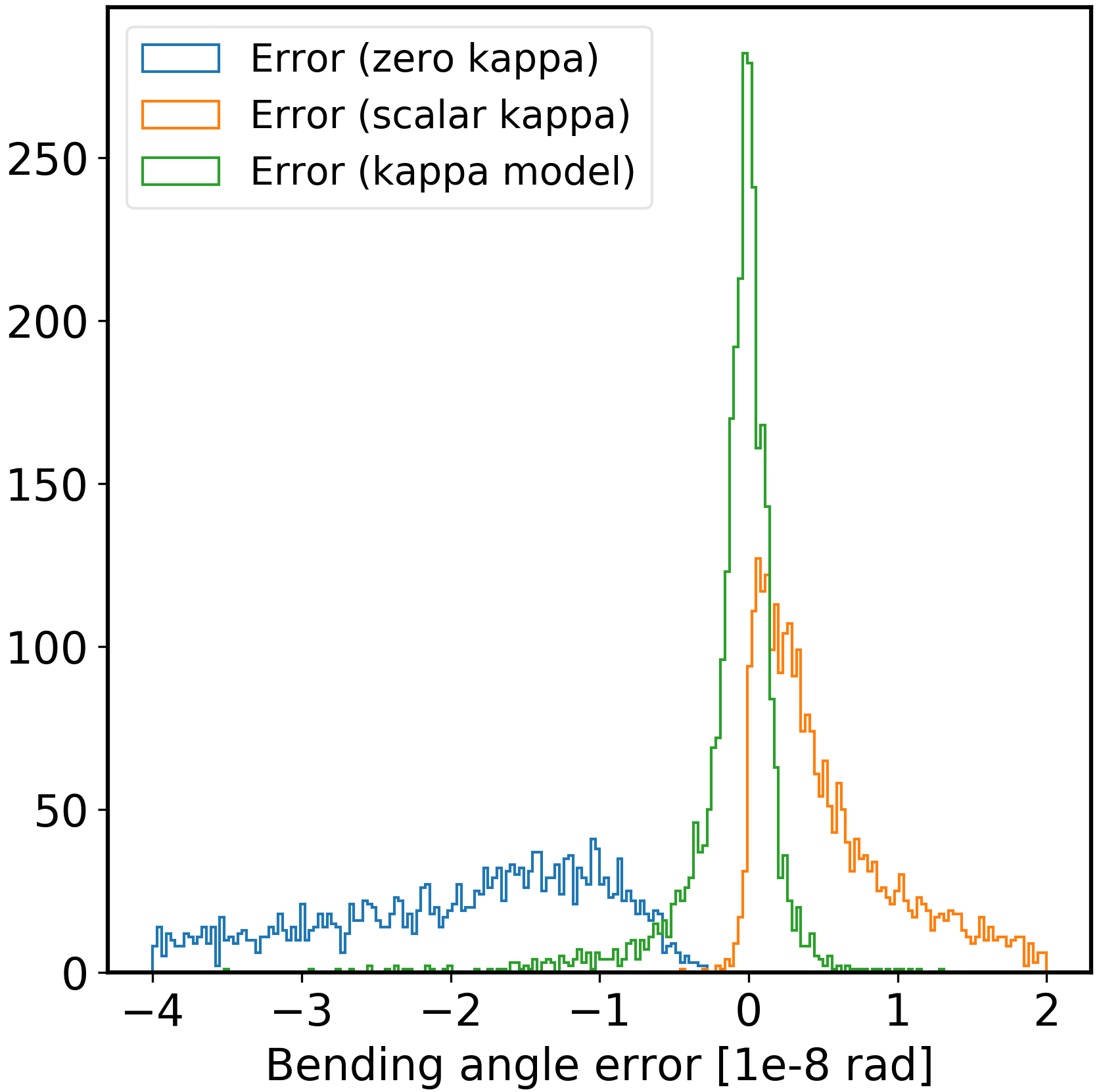
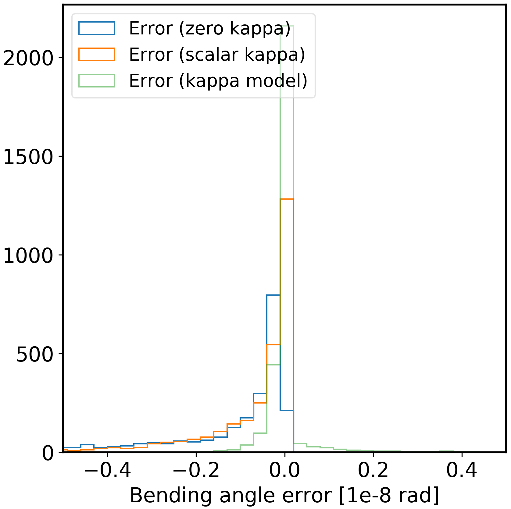
Figures 17 and 18 show histograms for residual bending angle for day and night respectively. In the daytime, the scal-κ is consistently too high and this results in an overcorrection of the bending angles and a positive bending angle bias (Table 7). Similarly, in the nighttime, scal-κ is too low and this results in a negative bending angle bias. However, in this case, the bending angles are already small and the impact of the choice of κ is less pronounced (Table 7). Conversely, the func-κ results in a negative bending angle bias in the daytime and positive bias at night. In both cases, the bending angle biases are significantly lower than those produced with scal-κ.
Many studies of ionospheric refraction of transionospheric radio waves have shown that, in addition to the level of ionisation, the shape of the vertical electron density profile plays a significant role, e.g. Jakowski et al. (1994) and Hoque and Jakowski (2008, 2010). It is important to remember that the functional model of κ has been created by fitting κ derived from NeQuick. NeQuick is based on the standard CCIR databases of foF2, foE and M3000F2 and therefore provides a reasonable median model of the F and E regions' peaks; however, it is not certain that NeQuick is a good median representation of the layer shapes. Furthermore, the κ model is derived from 1-D estimates of the bending angle and so does not take nonspherical structures into consideration. The approach, therefore, has been to model kappa with minimal complexity to avoid a close fitting to NeQuick that may be inappropriate in reality. Additional terms have been also trialled in the model (such as local time), but these have not shown any significant improvement of the model presented in this paper. Given the limitation of the ionospheric model and the bending angle estimation, the results are indicative that a simple kappa model may be used, but further testing with real data must be done to validate this.
Using the random selection of vertical profiles from the NeQuick the median κ has been shown to be 14 rad−1 and this is therefore an appropriate value for κ if it is to be represented by a single scalar. This value agrees well with the result from Healy and Culverwell (2015) and is in the range suggested by Danzer et al. (2015). Representing κ as a scalar has the advantage of simplicity and is appropriate if climate reprocessing centres are focused on ensuring that global average biases are removed. However, it has been demonstrated that such an approach can lead to significant differences in the residual bending angle bias between day and night. In the day, the results indicate that the bending angle bias switches sign from rad for no correction to rad for the scalar κ correction.
This limitation can be overcome using the simple κ function model. This approach does not require independent ionospheric measurements and so remains easy to implement. It should be noted that the κ model is based on a monthly median ionospheric model. Whilst this is a starting point it will be necessary to work with climate reprocessing centres to develop an effective validation strategies of the bending angle corrections. It would also be useful to assess the sensitivity of stratospheric climatologies to the bending angle bias and standard deviation bounds determined by this study. Furthermore, the magnitude of other error terms (i.e. non-symmetry; Zeng et al., 2016) should be assessed in light of these results.
The NeQuick variant used to produce the results in this paper can be requested from the Abdus Salam International Centre for Theoretical Physics (ICTP), Trieste, Italy.
The authors declare that they have no conflict of interest.
This article is part of the special issue “Observing Atmosphere and Climate with Occultation Techniques – Results from the OPAC-IROWG 2016 Workshop”. It is a result of the International Workshop on Occultations for Probing Atmosphere and Climate, Leibnitz, Austria, 8–14 September 2016.
This work was undertaken as part of a visiting scientist study funded by the
Radio Occultation Meteorology Satellite Application Facility (ROM SAF), which
is a decentralised processing centre under the European Organisation for the
Exploitation of Meteorological Satellites (EUMETSAT). The original NeQuick
Fortran code was provided by ITCP.
Edited by:
Anthony Mannucci
Reviewed by: Norbert Jakowski and one anonymous referee
Angrisano, A., Gaglione, S., Gioia, C., Massaro, M., and Troisi, S.: Benefit of the NeQuick Galileo Version in GNSS Single-Point Positioning, International Journal of Navigation and Observation, 2013, 302947, https://doi.org/10.1155/2013/302947, 2013.
Bilitza, D. and Reinisch, B. W.: International Reference Ionosphere 2007: Improvements and new parameters, J. Adv. Space Res., 42, 599–609, 2008.
Chu, Y.-H., Wu, K.-H., and Su, C.-L.: A new aspect of ionospheric E region electron density morphology, J. Geophys. Res., 114, A12314, https://doi.org/10.1029/2008JA014022, 2009.
Danzer, J., Scherllin-Pirscher, B., and Foelsche, U.: Systematic residual ionospheric errors in radio occultation data and a potential way to minimize them, Atmos. Meas. Tech., 6, 2169–2179, https://doi.org/10.5194/amt-6-2169-2013, 2013.
Danzer, J., Healy, S. B., and Culverwell, I. D.: A simulation study with a new residual ionospheric error model for GPS radio occultation climatologies, Atmos. Meas. Tech., 8, 3395–3404, https://doi.org/10.5194/amt-8-3395-2015, 2015.
Davies, K.: Ionospheric radio propagation, National Bureau of Standards, USA, 1965.
Di Giovanni, G. and Radicella, S. M.: An analytical model of the electron density profile in the ionosphere, Adv. Space Res., 10, 27–30, available at: http://linkinghub.elsevier.com/retrieve/pii/027311779090301F (last access: 8 August 2016), 1990.
Epstein, P. S.: Reflection of Waves in an Inhomogeneous Absorbing Medium, P. Natl. A. Sci. USA, 16, 627–637, 1930.
Hajj, G .A., Kursinski, E. R., Romans, L. J., Bertiger, W. I., and Leroy, S. S.: A Technical Description of Atmospheric Sounding By GPS, J. Atmos. Sol.-Terr. Phys., 64, 451–469, 2002.
Hardy, K. R., Hajj, G. A., and Kursinski, E. R.: Accuracies of atmospheric profiles obtained from GPS occultations, Int. J. Satell. Commun., 12, 463–473, https://doi.org/10.1002/sat.4600120508, 1994.
Healy, S. B.: Radio occultation bending angle and impact paramter errors caused by horizontal refractive index gradients in the troposhere: a simulation study, J. Geophys. Res., 106, 11875–11889, 2001.
Healy, S. B. and Culverwell, I. D.: A modification to the standard ionospheric correction method used in GPS radio occultation, Atmos. Meas. Tech., 8, 3385–3393, https://doi.org/10.5194/amt-8-3385-2015, 2015.
Healy, S. B. and Thépaut, J.-N.: Assimilation experiments with CHAMP GPS radio occultation measurements, Q. J. Roy. Meteor. Soc., 132, 605–623, https://doi.org/10.1256/qj.04.182, 2006.
Hoque, M. M. and Jakowski, N.: Estimate of higher order ionospheric errors in GNSS positioning, Radio Sci., 43, RS5008, https://doi.org/10.1029/2007RS003817, 2008.
Hoque, M. M. and Jakowski, N.: Higher order ionospheric propagation effects on GPS radio occultation signals, Adv. Space Res., 46, 162–173, available at: http://www.sciencedirect.com/science/article/pii/S0273117710001183 (last access: 16 October 2017), 2010.
Jakowski, N., Porsch, F., and Mayer, G.: Ionosphere-Induced Ray-Path Bending Effects in Precision Satellite Positioning Systems, Zeitschrift f. satellitengestützte Positionierung, Navigation und Kommunikation SPN, 1, 6–13, available at: http://elib.dlr.de/23702/ (last access: 16 October, 2017), 1994.
Kursinski, E. R., Hajj, G. A., Schofield, J. T., Linfield, R. P., and Hardy, K. R.: Observing Earth's atmosphere with radio occultation measurements using the Global Positioning System, J. Geophys. Res., 102, 23429–23465, 1997.
Mannucci, A. J., Ao, C. O., Pi, X., and Iijima, B. A.: The impact of large scale ionospheric structure on radio occultation retrievals, Atmos. Meas. Tech., 4, 2837–2850, https://doi.org/10.5194/amt-4-2837-2011, 2011.
Nava, B., Coisson, P., and Radicella, S.: A new version of the neQuick ionosphere electron density model, J. Atmos. Sol.-Terr. Phys., 70, 1856–1862, 2008.
Poli, P., Moll, P., Puech, D., Rabier, F., and Healy, S. B.: Quality Control, Error Analysis, and Impact Assessment of FORMOSAT-3/COSMIC in Numerical Weather Prediction, Terr. Atmos. Ocean. Sci., 20, 101, available at: http://tao.cgu.org.tw/index.php/articles/archive/space-science/item/817 (last acccess: 25 April 2017), 2009.
Poli, P., Healy, S. B., and Dee, D. P.: Assimilation of Global Positioning System radio occultation data in the ECMWF ERA-Interim reanalysis, Q. J. Roy. Meteor. Soc., 136, 1972–1990, https://doi.org/10.1002/qj.722, 2010.
Rawer, K.: Replacement of the Present Sub-Peark Plasma Density Profile by a Unique Expression, Adv. Space Res., 2, 183–190, 1983.
Rennie, M. P.: The impact of GPS radio occultation assimilation at the Met Office, Q. J. Roy. Meteor. Soc., 136, 116–131, https://doi.org/10.1002/qj.521, 2010.
Steiner, A. K., Hunt, D., Ho, S.-P., Kirchengast, G., Mannucci, A. J., Scherllin-Pirscher, B., Gleisner, H., von Engeln, A., Schmidt, T., Ao, C., Leroy, S. S., Kursinski, E. R., Foelsche, U., Gorbunov, M., Heise, S., Kuo, Y.-H., Lauritsen, K. B., Marquardt, C., Rocken, C., Schreiner, W., Sokolovskiy, S., Syndergaard, S., and Wickert, J.: Quantification of structural uncertainty in climate data records from GPS radio occultation, Atmos. Chem. Phys., 13, 1469–1484, https://doi.org/10.5194/acp-13-1469-2013, 2013.
Syndergaard, S.: On the ionosphere calibration in GPS radio occultation measurements, Radio Sci., 35, 865–883, https://doi.org/10.1029/1999RS002199, 2000.
Vorob'ev, V. V. and Krasil'nikova, T. G.: Estimation of the accuracy of the atmospheric refractive index recovery from the NAVSTAR system, USSR Physics of the Atmosphere and Ocean (Eng. Trans.), 29, 602–609, 1994.
Zeng, Z., Sokolovskiy, S., Schreiner, W., Hunt, D., Lin, J., and Kuo, Y.-H.: Ionospheric correction of GPS radio occultation data in the troposphere, Atmos. Meas. Tech., 9, 335–346, https://doi.org/10.5194/amt-9-335-2016, 2016.