2.1 The OMI sensor and O₂–O₂ 477 nm spectral band

The Dutch–Finnish OMI mission (Levelt et al., 2006) is a nadir-viewing push-broom imaging spectrometer launched on the National Aeronautics and Space Administration (NASA) Earth Observing System (EOS) Aura satellite. It delivers global coverage with a high temporal resolution of key air quality components derived from measurements of the backscattered solar radiation acquired in the UV–vis spectral domain (270–550 nm) with approximately 0.5 nm resolution. Based on a two-dimensional detector array concept, radiance spectra are simultaneously measured on a 2600 km wide swath within a nadir pixel size of 13×24 km² (28×150 km² at extreme off-nadir).

The O₂−O₂ 477 nm absorption band is currently operationally exploited by the OMI O₂−O₂ cloud algorithm (OMCLDO2) to derive effective cloud parameters (Acarreta et al., 2004; Veefkind et al., 2016). This spectral band directly measures the absorption of the visible part of the sunlight induced by the O₂–O₂ collision complex along the whole light path. A spectral fit, prior to the OMI effective cloud retrieval algorithm, is performed over the 460–490 nm spectral range to derive the continuum reflectance R_c (475 nm) and the O₂−O₂ slant column density $N_{{\mathrm{O}}_{\mathrm{2}}-{\mathrm{O}}_{\mathrm{2}}}^{\mathrm{s}}$. This spectral fit relies on the differential optical absorption spectroscopy (DOAS) approach (Platt and Stutz, 2008). $N_{{\mathrm{O}}_{\mathrm{2}}-{\mathrm{O}}_{\mathrm{2}}}^{\mathrm{s}}$ represents the O₂−O₂ absorption magnitude along the average light path through the atmosphere. This is the key input variable for the OMI ALH retrieval by the NN algorithm.

2.2 The OMI aerosol layer height neural network algorithm

The OMI ALH retrieval algorithm (Chimot et al., 2017) is based on the exploitation of $N_{{\mathrm{O}}_{\mathrm{2}}-{\mathrm{O}}_{\mathrm{2}}}^{\mathrm{s}}$ derived from the DOAS fit and relies on a NN approach. Here, the main elements of this algorithm are summarized, but for more details about their technical development and implementation, see Chimot et al. (2017).

This algorithm relies on how aerosols affect the length of the average light path along which the O₂−O₂ absorbs. $N_{{\mathrm{O}}_{\mathrm{2}}-{\mathrm{O}}_{\mathrm{2}}}^{\mathrm{s}}$ is then driven by the overall shielding or enhancement effect of photons by the O₂−O₂ complex in the visible spectral range due to the presence of particles. An aerosol layer located at high altitudes applies a large shielding effect on the O₂−O₂ located in the atmospheric layers below: i.e. the amount of photons coming from the top of the atmosphere (TOA) and reaching the lowest part of the atmosphere is reduced compared to an aerosol-free scene. This shielding effect is then larger when the aerosol layer is located at an elevated altitude than close to the surface.

The designed NNs belong to the family of machine learning and the artificial intelligence domain and rely on a multi-layer architecture, also named multilayer perceptron. The input and output variables are interconnected through a set of sigmoid functions present in the hidden layers and the synaptic weights W. For each single sigmoid function, two simple operations are performed: (1) a weighted sum of all the inputs given by the previous layer and (2) a transport of this sum through the sigmoid functions. The ALH retrieval problem then becomes a simple series of analytical functions.

For all the processed OMI scenes, aerosol profile is assumed as one single scattering layer (also called “box layer”) with a constant geometric thickness (100 hPa, or about 1 km). The particles included in this layer are homogeneous (i.e. same size and optical properties). ALH is then defined as the mid-altitude (a.s.l.) of this scattering layer. Furthermore, aerosol particles are assumed to cover the entire satellite observation pixel. The input layer contains seven parameters: viewing zenith angle θ, solar zenith angle θ₀, relative azimuth angle ϕ_r, surface pressure Ps, surface albedo A, aerosol optical thickness τ(550 nm), and the OMI $N_{{\mathrm{O}}_{\mathrm{2}}-{\mathrm{O}}_{\mathrm{2}}}^{\mathrm{s}}$. As explained in Chimot et al. (2017), a prior τ(550 nm) is required as input as both ALH and τ(550 nm) simultaneously affect $N_{{\mathrm{O}}_{\mathrm{2}}-{\mathrm{O}}_{\mathrm{2}}}^{\mathrm{s}}$ and need to be distinguished.

The optimal weights were estimated through a rigorous training task following the error back propagation technique and a training dataset that includes a set of representative situations for which inputs and outputs are well known. The quality of the training dataset was ensured by full physical spectral simulations, dominated by aerosol particles without clouds, generated by the Determining Instrument Specifications and Analyzing Methods for Atmospheric Retrieval (DISAMAR) software of KNMI (de Haan, 2011). Aerosol scattering is simulated by a Henyey–Greenstein (HG) scattering phase function Φ(Θ) parameterized by the asymmetry parameter g, which is the average of the cosine of the scattering angle (Hovenier and Hage, 1989). Aerosols were specified for a standard case, assuming fine particles with a unique value of the extinction Ångström exponent α = 1.5 and g=0.7. In order to investigate the assumptions related to the aerosol single scattering albedo ω₀ properties, two training datasets were generated with a different typical value: one with ω₀ = 0.95 and one with ω₀ = 0.9 in the visible spectral domain. Therefore, two OMI ALH NN algorithms were created, one for each aerosol ω₀ values.

The aerosol models in the training database were based on a HG scattering phase function for two reasons. First, both Chimot et al. (2017) and this paper are exploratory studies focusing on the potential of exploiting the O₂−O₂ spectral band for aerosol retrievals from a satellite sensor. Second, our first long-term objective is the potential use of the ALH parameter for future tropospheric NO₂ and similar trace gas retrievals over cloud-free scenes. Several studies emphasized that ALH is the key variable affecting the length of the average light path in the computation of the related air mass factor (AMF) computation through the DOAS approach (Boersma et al., 2004; Castellanos et al., 2015; Chimot et al., 2016). This is because the only quantity that is relevant for absorption by trace gases in the visible is the average light path distribution, i.e. the distribution of distances travelled by photons in the atmosphere before leaving the atmosphere. The absolute radiance at the TOA is less important. The second variable of interest is τ. This average light path distribution is mostly governed by ω₀ and g, and of course ALH and τ, and much less by details in the phase function. Studies by Leitão et al. (2010), Castellanos et al. (2015), and Chimot et al. (2016) showed the lower sensitivity of the AMF to α, ω₀, and g. These scattering parameters are included in HG scattering, and therefore this parameterized phase function can be used for AMF calculations. At this level and with respect to these mentioned objectives, it is then assumed one does not need to define more realistic aerosol models for every single OMI pixel. With g=0.7, the HG function is known to be smooth and reproduce the Mie scattering functions reasonably well for most of aerosol types, in particular for spherical particles (e.g. nitrate, sulfate) (Dubovik et al., 2002). Such an approach is used for the preparation of the operational ALH retrieval algorithms for Sentinel-4 and Sentinel-5 Precursor (Leitão et al., 2010; Sanders et al., 2015; Colosimo et al., 2016; Nanda et al., 2018) and for various explicit aerosol corrections in the AMF calculation when retrieving trace gases, such as tropospheric NO₂, over urban and industrial areas dominated by anthropogenic pollution, for example in eastern China (Spada et al., 2006; Wagner et al., 2007; Castellanos et al., 2015; Vlemmix et al., 2010). The potential impact of the modelled scattering phase discussion is kept in mind and further discussed in Sect. 4.4. However, reperforming the whole NN training process with more complex particle shape models is computationally very demanding and beyond the scope of this paper. Instead, more elements on specific error analysis are further discussed in Sect. 4.

Maximum seasonal differences between the LIdar climatology of Vertical Aerosol Structure for space-based lidar simulation studies (LIVAS) and 3-year OMI ALH, over cloud-free scenes in north-eastern Asia with MODIS τ(550 m)≥1.0, are in the range of 180–800 m (Amiridis et al., 2015; Chimot et al., 2017). The previous extended sensitive study has shown the following. (a) Due to the nature of the O₂−O₂ spectral band, a minimum particle load (i.e. τ(550 nm)=0.5) is required to be able to exploit the aerosol signal as, below this threshold, low amounts of aerosols have negligible impacts on $N_{{\mathrm{O}}_{\mathrm{2}}-{\mathrm{O}}_{\mathrm{2}}}^{\mathrm{s}}$ shielding and lead to high ALH bias. (b) The aerosol model assumptions are the most critical, in particular ω₀, as they may affect ALH retrieval uncertainty up to 660 m. (c) In addition, potential aerosol residuals in the prior surface albedo may impact up to 200 m. (d) An accuracy of 0.2 is required on prior τ(550 nm) to limit ALH bias close to zero when τ(550 nm)≥1.0 and below 500 m for τ(550 nm) values close to 0.6.

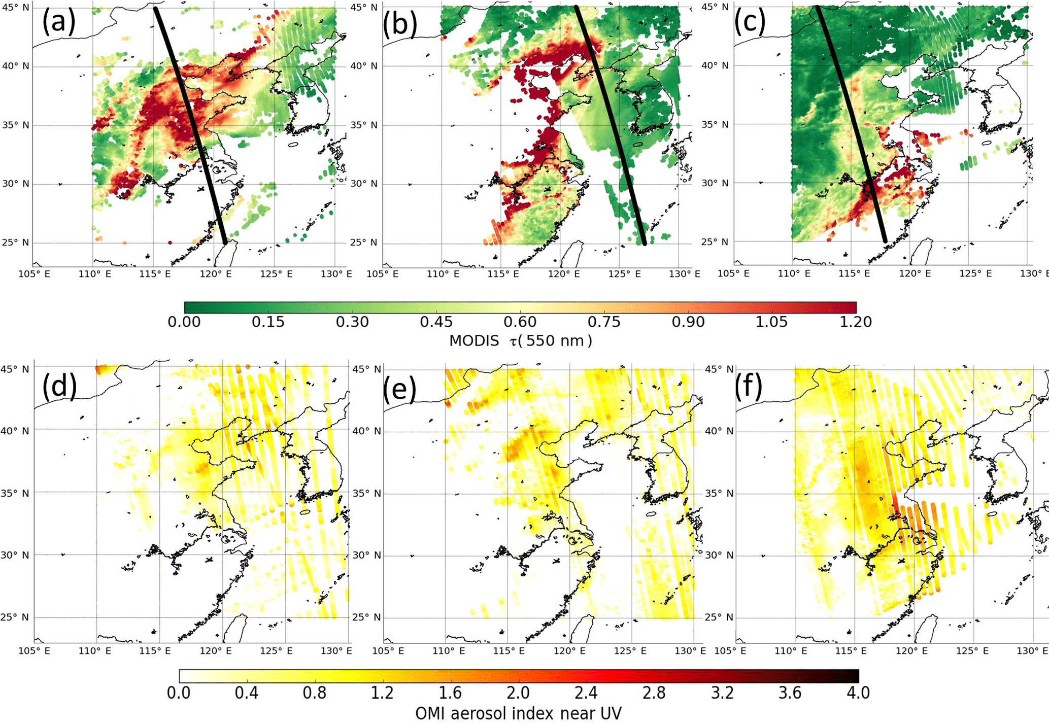
Figure 1Maps of Aqua MODIS τ(550 nm) from the combined DT and DB Collection 6 (see Sect. 2.3) and collocated OMI aerosol index from near-UV (UVAI) values (see Sect. 3) over cloud-free scenes for the urban and industrialized cases in eastern China. The dark thick lines represent the track of CALIPSO space-borne sensor over the selected case studies: (a, d) 2 October 2006, (b, e) 6 October 2006, and (c, f) 1 November 2006.

Download

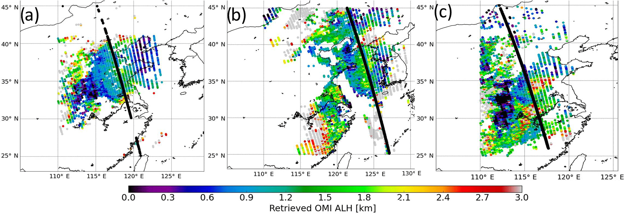
Figure 2Maps of retrieved OMI aerosol layer height (ALH) from all the cloud-free pixels collocated with Aqua MODIS τ(550 nm) (see Fig. 1). The dark thick lines represent the track of CALIPSO space-borne sensor over the selected case studies: (a) 2 October 2006, (b) 6 October 2006, and (c) 1 November 2006.

Download

2.3 The CALIOP and MODIS aerosol products

CALIOP sensor is a standard dual-wavelength elastically backscattered lidar on board the CALIPSO satellite platform, flying since 2006. Equipped with a depolarization channel at 532 nm, it probes the aerosol and cloud vertical layers, from the surface to 40 $\mathrm{km}\mathrm{a}.\mathrm{s}.\mathrm{l}.$, with a high vertical resolution (Winker et al., 2009). Level 1 scientific data products, distributed by the Atmospheric Science Data Center (ASDC) of NASA, include the lidar calibrated and geolocated measurements of high-resolution vertical profiles (between 30 and 60 m in the troposphere) of the aerosol and cloud attenuated backscatter coefficients at 532 and 1064 nm with horizontal resolutions of 1∕3, 1, and 5 km (Winker et al., 2009).

The CALIOP aerosol L2 product contains the retrieved aerosol backscatter and extinction coefficient profiles at 532 and 1064 nm, for each identified and well-located aerosol layer, at 5 km horizontal resolution. These retrievals are performed after calibration, range correction, feature detection and classification, and assumptions on lidar extinction-to-backscattering ratio (Winker et al., 2009; Young and Vaughan, 2009).

The MODIS spectrometer was launched on the NASA EOS Aqua platform in May 2002 and has been delivering continuous images of the Earth in the visible, solar, and thermal infrared approximately 15 min prior to OMI. The considered Aqua MODIS L2 aerosol product is the Collection 6 of MYD04_L2, based on the Dark Target (DT) and Deep Blue (DB) algorithms with a high enough quality assurance flag and an improved calibration of the instrument (Levy et al., 2013). While the MODIS measurement is acquired at the resolution of 1 km, the used MODIS aerosol τ(550 nm) is at 10 km × 10 km, relatively close to the OMI nadir spatial resolution. The expected uncertainties of MODIS τ(550 nm) are about $\pm \mathrm{0.05}+\mathrm{15}\mathit{\%}$ over land for DT (Levy et al., 2013) and about ±0.03 on average for DB (Sayer et al., 2013).

3.1 Methodology

OMI ALH retrievals are here obtained using MODIS L2 aerosol τ(550 nm) from the combined DT and DB product as prior input, collocated within a distance of 15 km and where τ(550 nm)≥0.55 (see Sect. 2.2). Mitigating the probability of cloud contamination within the OMI pixel is one of the first criteria for a successful ALH retrieval. For that purpose, we rely on the availability of the MODIS aerosol product with the highest quality assurance flag ensuring that Aqua MODIS τ(550 nm) is exclusively estimated when a sufficient high amount of cloud-free sub-pixels is available (i.e. at the MODIS measurement resolution of 1 km) (Levy et al., 2013). However, since this may be not completely representative of the atmospheric situation of the OMI pixel, two thresholds are added for each collocated OMI–MODIS pixel: the geometric MODIS cloud fraction to be smaller than 0.1, and the effective OMI cloud fraction lower than 0.2. For this last parameter, it was shown that values higher than 0.3 are generally likely contaminated by clouds, while values between 0.1 and 0.2 may be cloud-free but contain a substantial amount of very scattered particles that increase the scene brightness (Boersma et al., 2011; Chimot et al., 2016).

The ALH retrievals are applied to the OMI DOAS O₂−O₂ observations, available in the last reprocessed OMCLDO2 product version (Acarreta et al., 2004; Veefkind et al., 2016). A temperature correction is taken into account on the $N_{{\mathrm{O}}_{\mathrm{2}}-{\mathrm{O}}_{\mathrm{2}}}^{\mathrm{s}}$ variable, using the information available in the OMCLDO2 product, which is itself based on the temperature profiles of the National Centers for Environmental Prediction (NCEP) analysis data (Veefkind et al., 2016).

The selected case studies include (1) urban and industrial aerosol pollution over eastern China during 3 days between October and November 2006, (2) large wildfire episodes in South America in August 2006 and September 2007 and in eastern Russia in August 2010 and June 2012, and (3) a Saharan dust transport over sea in June 2012. OMI ALH retrievals are compared with collocated CALIOP products within a distance of 50–100 km for the cases over eastern China and South America and 300 km for eastern Russia. The larger OMI–CALIOP distance over these two last regions is due to the so-called “row anomaly”, which has been significantly perturbing OMI measurements of the earthshine radiance at all wavelengths since 2009. This leads to a reduced number of valid OMI ground pixels close to the CALIOP track. Details are given at http://www.knmi.nl/omi/research/product/rowanomaly-background.php (last access: 8 August 2010).

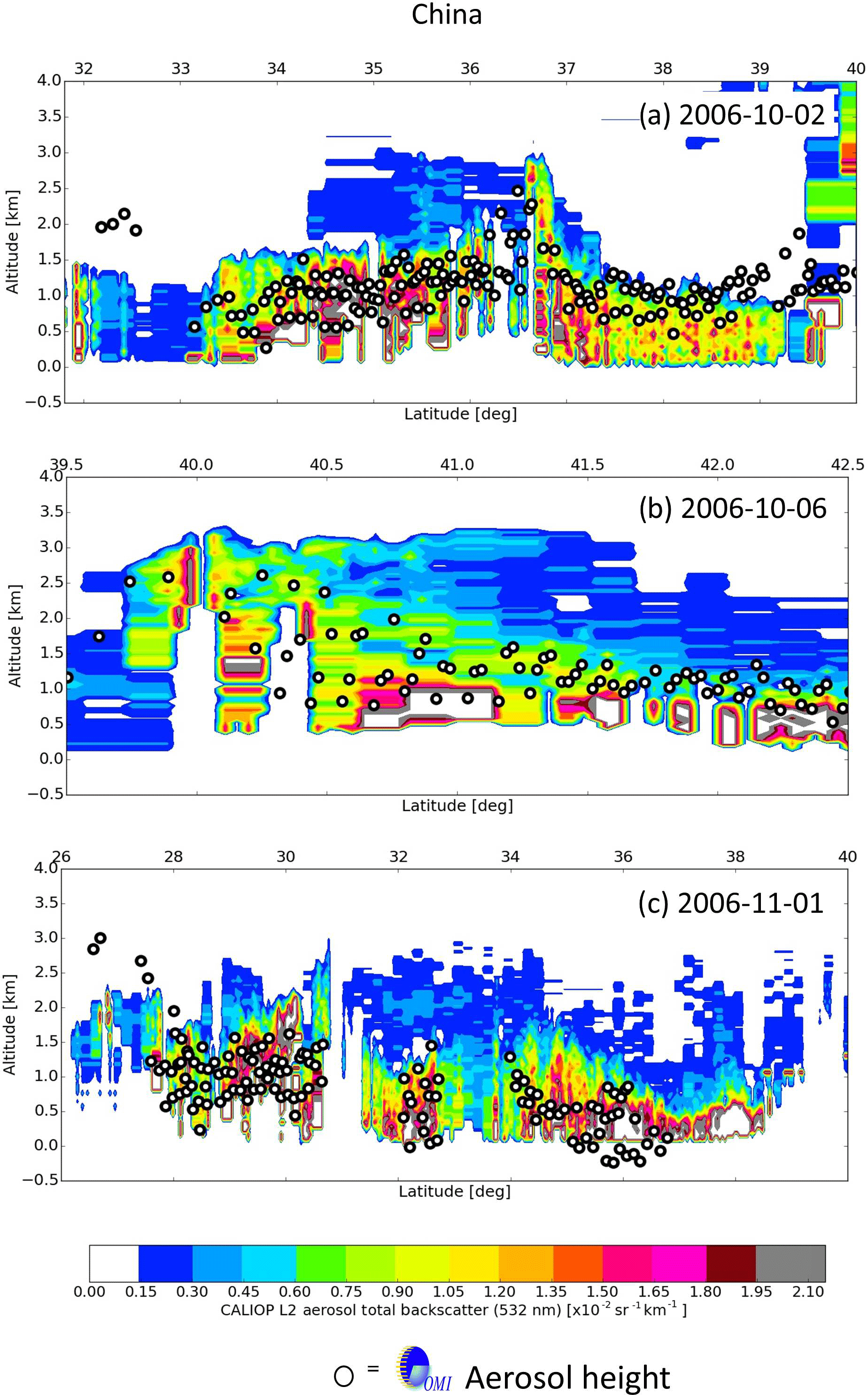
Figure 3Retrieved OMI ALH compared with vertical profile of aerosol total backscatter coefficient (532 nm) from the CALIOP L2 product. Maximal distance between OMI pixels and CALIOP ground track is 50 km. Only cloud-free OMI pixels, collocated with Aqua MODIS Collection 6 aerosol cells, τ(550 nm)≥0.55 (from the MODIS DT and DB algorithms), are selected: (a) 2 October 2006, (b) 6 October 2006, and (c) 1 November 2006.

Download

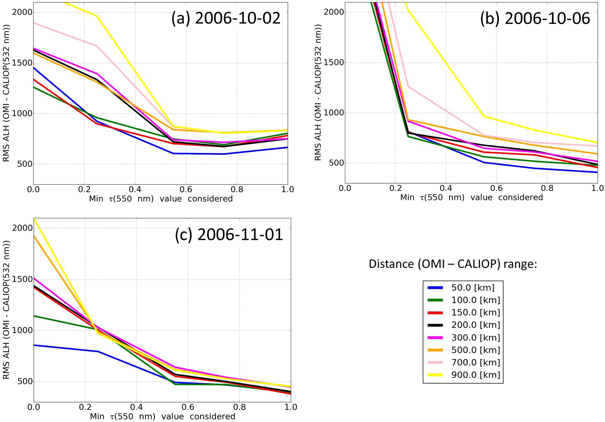
Figure 4Root-mean-square (RMS) deviation between collocated retrieved OMI ALH and derived CALIOP ALH (532 nm) (see Sect. 4.1) for urban and industrialized cases over eastern China as a function of minimum MODIS τ(550 nm) and distance between OMI and CALIOP ground pixels: (a) 2 October 2006, (b) 6 October 2006, and (c) 1 November 2006.

Download

Figure 5Scatter-plot of collocated retrieved OMI ALH and derived CALIOP ALH (532 nm) (see Sect. 4.1) for urban and industrialized cases over eastern China as a function of MODIS τ(550 nm). Distance between OMI and CALIOP pixels is 50 km: (a) 2 October 2006, (b) 6 October 2006, and (c) 1 November 2006.

Download

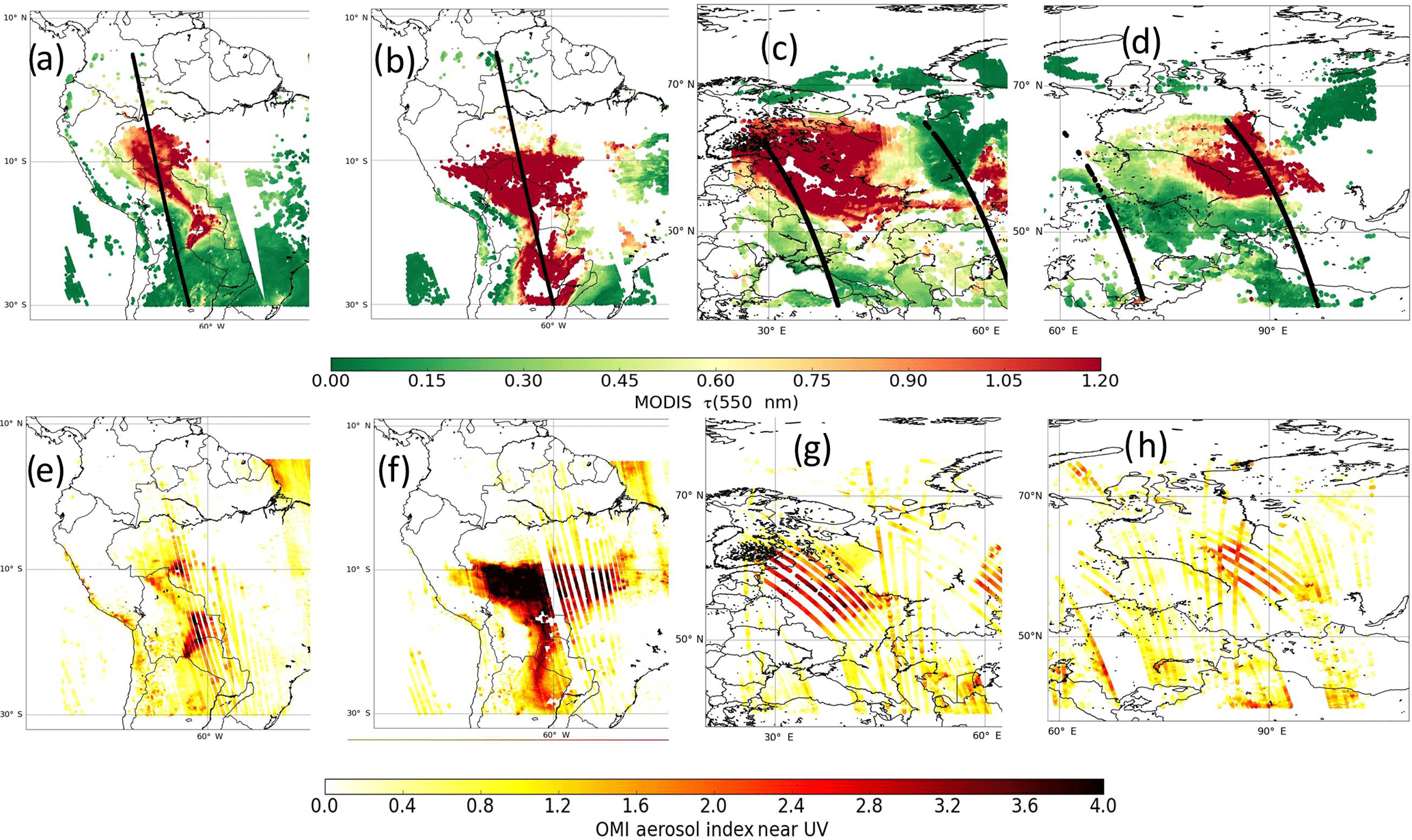
Figure 6Maps of Aqua MODIS τ(550 nm) from the combined DT and DB Collection 6 (see Sect. 2.4) and collocated OMI aerosol index from near-UV (UVAI) values (see Sect. 3) over cloud-free scenes and intensive biomass burning episodes. The dark thick lines represent the track of CALIPSO space-borne sensor over the selected case studies: (a, e) South America on 24 August 2006, (b, f) South America on 30 September 2007, (c, g) eastern Russia on 8 October 2010, and (d, h) eastern Russia on 23 June 2012.

Download

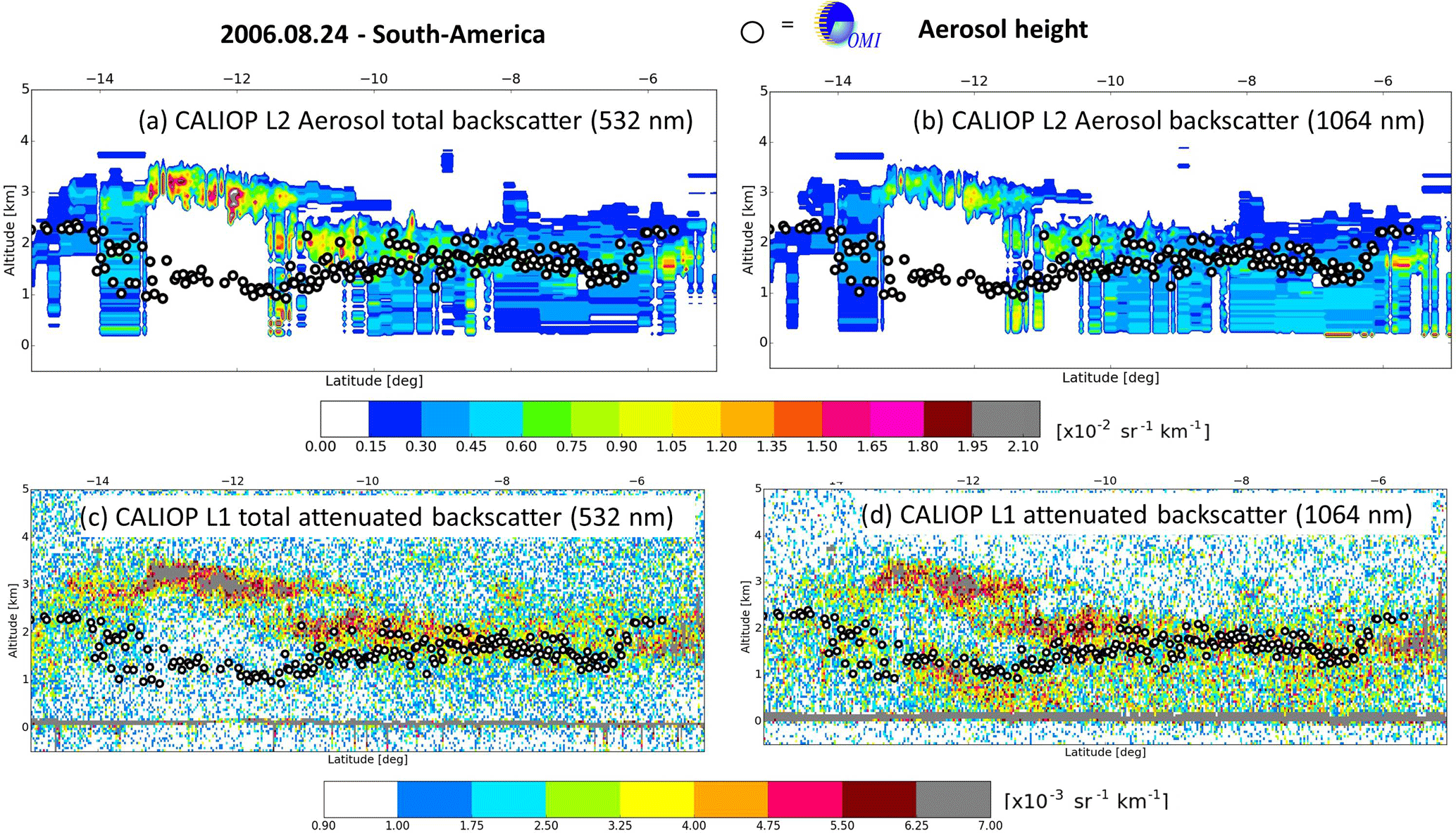
Figure 7Retrieved OMI ALH compared with CALIOP along-track vertical profile observations for biomass burning case over South America: (a) CALIOP L2 aerosol total backscattering (532 nm), (b) CALIOP L2 aerosol backscattering (1064 nm), (c) CALIOP L1 attenuated backscattering (532 nm), and (d) CALIOP L1 attenuated backscattering (1064 nm).

Download

Figure 8Retrieved OMI ALH compared with CALIOP L1 along-track vertical profile observations (532 and 1064 nm) for biomass burning cases: (a, b) 30 September 2007 in South America, (c, d) 8 August 2010 in eastern Russia, and (e, f) 23 June 2012 in eastern Russia.

Download

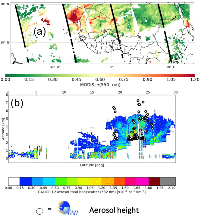
Figure 9Elevated layer due to a Saharan dust outbreak transported to western Mediterranean region over sea on 19 July 2007. (a) Map of Aqua MODIS τ(550 nm) from the combined DT and DB Collection 6 (see Sect. 2.3). (b) Retrieved OMI ALH compared with vertical profile of aerosol total backscatter coefficient (532 nm) from the CALIOP L2 aerosol total backscatter (532 nm) associated with the second left CALIPSO track over sea in Fig. 9a.

Download

For each study case, the most likely suitable NN algorithm (see Sect. 2.2) is selected by hand. We decided to rely on (1) the OMI UV aerosol absorbing index (UVAI) and (2) their well-known absorbing properties (according to the literature) in the visible spectral range in order to approximate the assumption on aerosol ω₀ at the visible (460–490 nm) spectral wavelengths. OMI UVAI is derived by the OMI near-UV aerosol algorithm (OMAERUV) in the 330–388 nm spectral band (Torres et al., 2007). It allows us to detect and distinguish UV absorbing from scattering aerosols through the measured change of spectral contrast, with respect to a pure Rayleigh atmosphere. Weakly absorbing or large non-absorbing particles are associated with near-zero or negative UVAI values. A threshold of 1 on UVAI is then specified to detect absorbing particles in the UV and then potentially in the visible.

3.2 Urban aerosol pollution

Fossil-fuel combustion is the main source of air pollution in the large urban and industrialized area of eastern China. With decreasing temperatures in autumn, coal-burning power plant activity is increased due to a higher energy consumption of heating systems. Consequently, excessive amounts of aerosol particles and their precursors are emitted (Chameides et al., 1999). Moreover, crop residue burning in the agricultural areas of eastern Asia may enhance aerosol concentrations (Xue et al., 2014). Mineral dust particles, from the Taklamakan and Gobi deserts between middle of spring and end of autumn, are transported through westerly winds (Eck et al., 2005; Proestakis et al., 2017). Collectively, the mix of all these pollutants contributes to the formation of regional brown hazes greatly threatening public health, over the North China Plain during the dry season (from October to March). They have been frequently detected by satellite and ground-based observations (Ma et al., 2010).

Figure 10Simulated ALP retrievals, based on noise-free synthetic spectra with aerosols, as a function of true τ(550 nm). All the retrievals are achieved with the NN algorithm trained with aerosol ω₀ = 0.9 and true prior τ(550 nm) value. The assumed geophysical conditions are temperature, H₂O, O₃, and NO₂ from climatology mid-latitude summer, θ₀ = 25^∘, θ = 45^∘, and P_s = 1010 hPa. The reference aerosol scenario assumes fine scattering particles (α = 1.5, g = 0.7) and two aerosol ω₀ values: 0.9 and 0.8. Its location is depicted by the grey box, between 700 and 800 hPa.

Download

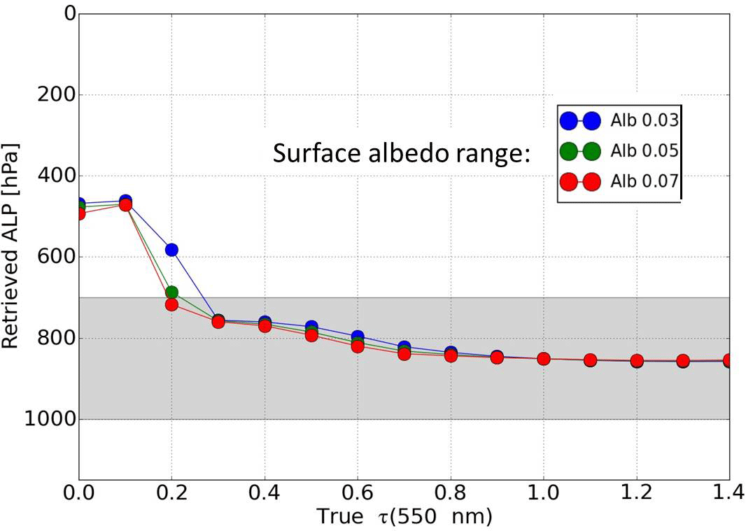
Figure 11Same as Fig. 10 but with one unique aerosol ω₀ value (=0.9) and a larger geometric extension of the aerosol layer included in the simulated spectra, i.e. between 700 and 1000 hPa.

Download

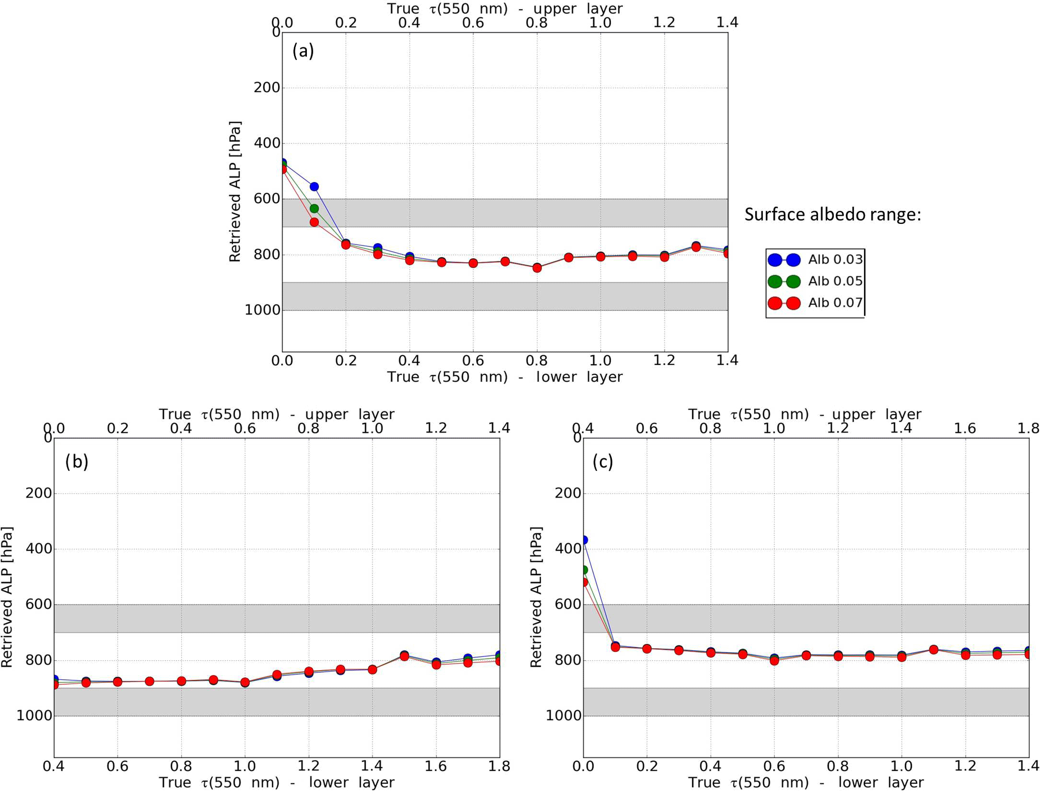
Figure 12Same as Fig. 10 but with one unique aerosol ω₀ value (=0.9) and two separate aerosol layers included in the simulated spectra. The bottom x axis corresponds to the τ(550 nm) value of the lower layer, while the top x axis is the τ(550 nm) value of the upper layer. Both layers have same geometric thickness (i.e. 100 hPa). The first is located between 600 and 700 hPa, and the second is between 900 and 1000 hPa. (a) Both aerosol layers have same optical properties and τ(550 nm) values. (b) Both aerosol layers have same optical properties but different τ(550 nm) values: the lower layer has systematically a higher τ(550 nm) (i.e. +0.4 for each scenario). (c) Both aerosol layers have same optical properties but different τ(550 nm) values: the upper layer has systematically a higher τ(550 nm) (i.e. +0.4 for each scenario).

Download

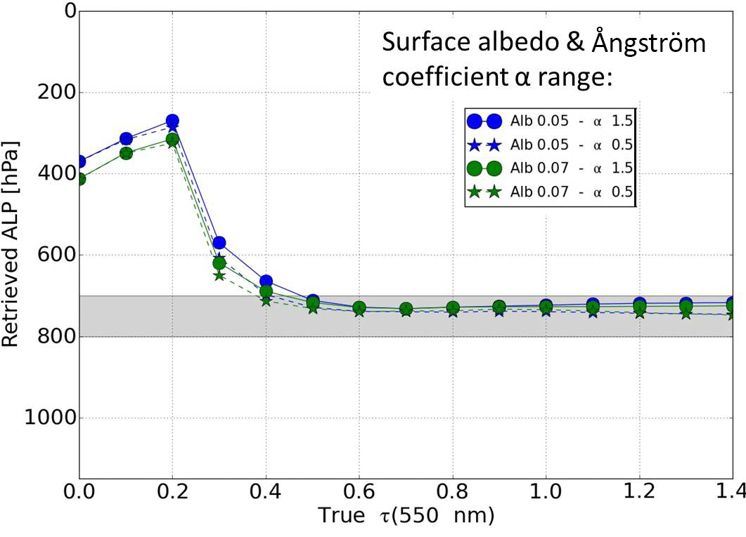
Figure 13Same as Fig. 10 but with one unique aerosol ω₀ value (=0.95) and two aerosol α (1.5 and 0.5) in the reference aerosol scenarios. ALP retrievals are estimated from the NN algorithm trained with aerosol ω₀=0.95 similarly to the desert dust case in Sect. 3.4.

Download

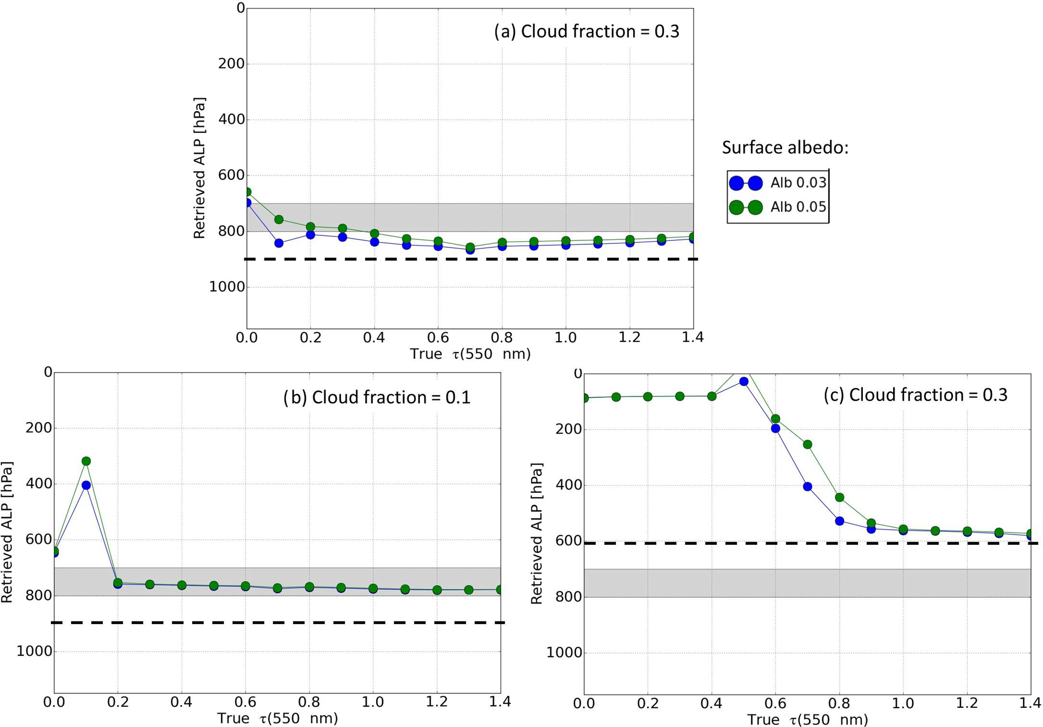
Figure 14Same as Fig. 10 but with one unique aerosol ω₀ value (0.9) and the inclusion of a cloud (dashed thick black line) in addition to the aerosol layer. The cloud reflectance is simulated via a simple opaque (cloud albedo of 0.8) and Lambertian layer. (a) Effective cloud fraction of 0.3 and cloud pressure of 900 hPa. (b) Effective cloud fraction of 0.1 and cloud pressure of 900 hPa. (c) Effective cloud fraction of 0.3 and cloud pressure of 600 hPa.

Download

Three typical days between October and November 2006 in eastern China were selected to illustrate the performance of the NN algorithm over scenes with strong urban aerosol pollution: day 1 of 2 October 2006, day 2 of 6 October 2006, and day 3 of 1 November 2006. As illustrated by the maps in Fig. 1, these days are characterized by high τ values over land as shown by Aqua MODIS: τ(550 nm) in the range of 0.5–1.6 in October 2006, and 0.5–1.3 in November 2006. Lin et al. (2015) estimated ω₀ values in summer (and likely beginning of autumn) in the range of 0.94–0.96 in the visible. This is likely a consequence of lower black carbon particle amounts at that time (compared to winter and spring) and a high dominance of anthropogenic particles such as nitrate and sulfate. These particles may also be mixed, in parts, with desert dust. Consistently, OMI UVAI depicts for the selected days values lower than or close to 1 (see Fig. 1). Therefore, we use the NN algorithm trained with ω₀=0.95 assuming low abundance of UV and visible absorbing particles.

Figure 2 depicts the spatial distribution of retrieved OMI ALH for all the selected collocated OMI–MODIS pixels, with a variability between 0.5 and 3 km. The CALIPSO suborbital tracks were mostly located inland in days 1 and 3 and between inland and over sea in day 2 (see Fig. 1 and Fig. 2). The aerosol layers in the CALIOP L2 product, based on the total backscatter coefficients (532 nm), are generally located between the surface and 1.5 km height (see Fig. 3). Maximum top heights do not exceed 2 km on 6 October 2006 or 3 km on the 2 other days. Collocated OMI ALH are mostly located in the middle aerosol layers and rarely exceed the top and bottom layer limits (see Fig. 2). Overall, for the 3 selected days, the OMI NN retrievals reproduce the spatial CALIOP L2 patterns. On 2 October 2006 in particular, OMI ALH remains relatively stable at the average altitude of 1 km, within the CALIOP L2 aerosol layers (see Fig. 3a). Only at the latitude 36.5^∘ N do both products simultaneously show an increased altitude close to 3 km. On the 2 other selected days, OMI ALH and CALIOP L2 show simultaneously descending slopes from south to north: a slope of about 2 km over 2.5^∘ latitude on 6 October 2006 and around 1.5 km over 8^∘ latitude on 1 November 2006 (see Fig. 3b and c).

An equivalent CALIOP L2 ALH can be derived by calculating an aerosol extinction weighted average altitude as follows:

where σ(l) is the CALIOP aerosol extinction (532 nm) of the vertical layer l defined by its mid-altitude h(l).

In Fig. 4, root-mean-square deviation (RMSD) between OMI and CALIOP L2 ALH lies in the range of 462–648 m when the maximum distance between the selected OMI and CALIOP ground pixels is lower than 50 km and with collocated MODIS τ(550 nm)≥0.55 (see Fig. 3). Associated bias values (i.e. average difference between OMI and CALIOP ALH per day) are between −86 and −128 m. These results significantly deteriorate, firstly when specifying a lower threshold on collocated MODIS τ(550 nm) (e.g. RMSD ≥1000 m with all MODIS τ(550 nm) values included) and secondly with a more flexible distance criterion (e.g. RMSD in the range of 594–888 m with a maximum distance of 500 km between the selected OMI and CALIOP ground pixels). The relatively low impact, noticed here, on the distance between OMI and CALIOP pixels is probably related to the large spatial extent of aerosol plumes and their relative spatial homogeneity. The impact of distance between collocated OMI–CALIOP pixels would be more detrimental over scenes with smaller and/or more heterogeneous plumes. Figure 5 shows the one-to-one comparison between OMI and CALIOP L2 ALH within a distance of 50 km per case study and as a function of associated MODIS τ(550 nm). The correlation coefficient (R) between OMI and CALIOP ALH varies per day, between 0.4 and 0.6 for all scenes with MODIS τ(550 nm)≥0.55.

3.3 Smoke and absorbing aerosol pollution from biomass-burning

Intensive biomass burning releases large amounts of carbonaceous and black carbon aerosols. The resulting dense smoke layers have a predominance of fine and strongly light-absorbing particles, especially in both the UV and visible spectral ranges. Combined with large τ values, this yields large light extinction and Ångström exponents (≥1.5) (Torres et al., 2013; Wu et al., 2014). Figure 6 shows the location and associated MODIS τ(550 nm) and OMI UVAI values for the selected biomass burning episodes: the two first events are over South America on 24 August 2006 and 30 September 2007; the two last events are over eastern Russia on 8 August 2010 and 23 June 2012. Due to the very high load of absorbing particles with MODIS τ(550 nm≥1.1), OMI UVAI values are generally higher than 2 and can locally reach 4, suggesting the use of the NN algorithm trained with ω₀=0.9 (see Fig. 6).

Several studies have identified loss of sensitivity of CALIOP attenuated backscatter profile measurements at 532 nm over scenes with dense smoke layers, such as over Canadian boreal and Amazonian fire events (Kacenelenbogen et al., 2011; Torres et al., 2013; Wu et al., 2014). Light extinction due to these layers is much larger at 532 nm than at 1064 nm (Pueschel and Livingston, 1990). Since CALIOP does not directly measure the aerosol backscattering but rather the attenuated backscattering, the range-dependent reduction in CALIOP lidar signals due to attenuation occurs more rapidly in the short wavelengths. Therefore, over scenes with heavy smoke particle loads, the attenuated backscatter coefficients (532 nm) in the lower part of the aerosol layer fall below the CALIOP's detection threshold, preventing the identification of the full vertical extent of the aerosol layers (from the top to the bottom). Being a down-looking observation lidar system, CALIOP tends then to mostly detect the top height compared to the base height of the aerosol layer as the laser's energy undergoes substantial attenuation when the beam travels through an optically thick layer (Vaughan et al., 2005; Kim et al., 2013). Therefore, the identified layers that are fully attenuated at 532 nm in the L1 product are filtered out in the L2 product. As a consequence of this filtering, CALIOP's τ of smoke layers is generally underestimated due to an overestimation of the layer base altitude (Wu et al., 2014; Kim et al., 2013).

Figure 7 depicts an example of the loss of sensitivity for a biomass burning case in South America. The CALIOP aerosol total backscatter (532 nm) and backscatter (1064 nm) coefficients in the L2 product mostly show the top layer of carbonaceous aerosols in the range of 3–4 km altitude with maximum thickness of 1 km, between 14 and 11^∘ S (see Fig. 7a and b). We found that the layers located below are flagged as totally attenuated at the wavelength of 532 nm, according to the CALIOP vertical feature mask. On the northernmost end of the detected plume, the aerosol load is around 2 km height. In contrast, the CALIOP L1 attenuated backscatter (1064 nm) profile detects an aerosol layer between the surface and 1.5 km, at the latitudes 11–14^∘ S. This layer is not observed by the CALIOP L1 total attenuated backscatter (532 nm) profile (see Fig. 7c and d) likely due to a better sensitivity of this channel to the particles located close to the surface.

The case of 24 August 2006 over South America shows the retrieved OMI ALH being well located, i.e. below the first elevated aerosol layer (at about 3 km) and at the top of the second aerosol layer, close to the surface (see Fig. 7d). Contrary to the CALIPSO L1 measurement (532 nm), our retrievals based on OMI visible measurements are not restricted to the top of the smoke or absorbing layer but correctly match with the middle of the layers detected by CALIPSO L1 (1064 nm). The reason that our OMI ALH seems closer to the top of the second layer may be due to a higher aerosol load and/or different layer properties (see Section 4.2).

Figure 8 shows that similar full CALIOP attenuation processes occur with the other selected biomass burning cases. The CALIOP L1 total attenuated backscatter (532 nm) vertical profiles mostly correlate with the top of the detected aerosol layers, while the CALIOP L1 attenuated backscatter (1064 nm) profiles reveal lower layers. On days of 30 September 2007 and 8 August 2010, the top layers are at elevated altitudes (higher than 3 km), while the lower ones extend from the surface to 1–2 km. On the last day, 23 June 2012, the top layer is lower (between 1 and 2 km). Similarly, all the OMI ALH retrievals are not restricted to the top layers but match, most of the time, with the middle of the layers, sometimes a bit closer to the base of the top layer or the top of the bottom layer. This may depend on the differences in terms of AOD and/or optical properties of each layer (see Sect. 4.2). In addition, it is worth noting the similar vertical variability (around 500 m) on 30 September 2007 in South America at the latitudes 8–15^∘ S and the remarkable descending slope, on 23 June 2012 in eastern Russia, from north to south at the latitudes 56–58^∘ S present in both OMI ALH and CALIOP L1 products.

Three reasons may explain why OMI visible spectra allow us to probe an entire absorbing aerosol layer, contrary to the active satellite visible measurement of CALIOP: (1) OMI measurements rely on the sun irradiance, which is much more intense than the laser pulse of CALIOP; (2) OMI measurements are largely issued from multiple scattering effects occurring at different altitudes, allowing a higher number of photons to reach the lower atmospheric layers; (3) the relatively higher signal-to-noise ratio (SNR) of OMI likely allows us to better detect and exploit the upcoming signal from smoke layers. In contrast, contributions of multiple scattering to the CALIOP backscattered signals are lower than single scattering effects within moderately dense dust layer and insignificant within smoke aerosol extinction (Winker, 2003; Liu et al., 2011). Furthermore, retrieving vertical profile of smoke layers from CALIOP requires a high aerosol extinction threshold due to the large associated lidar ratio and thus low SNR (Winker et al., 2013).

3.4 Desert dust transport

The case illustrated in Fig. 9a is a large desert dust plume over ocean surface, with MODIS τ(550 nm) values up to 1.1, released from the Sahara and transported through westerly winds along the African coast. It occurred in summer on 19 July 2007. Since the Sahara is the most important source of mineral particles, associated dust aerosols include hematite and other iron oxides. Spectrally, desert dust is a UV-absorbing particle but quite highly scattering in the visible (contrary to smoke) and longer wavelengths, leading to the appearance of relatively bright plumes (light brown) over the dark marine surface from a satellite point of view. The NN algorithm trained with aerosol ω₀=0.95 is therefore used here.

The vertical profile of CALIOP L2 aerosol total backscatter (532 nm) shows elevated layers, ranging from 1–2 km at 15^∘ S to 3–6 km at 23^∘ S (see Fig. 9b). Such a slope likely results from large-scale circulation governed by subtropical subsidence of the Intertropical Convergence Zone's northern branch, dry air from the desert, and the Saharan intense sensible heating effect perturbing the temperature inversion layers and thus creating convection uplifting dust from the surface (Prospero and Carlson, 1981). Generally, the OMI ALH results are consistent with CALIOP observations, with elevated values lying between 2 and 7 km. They are mostly located in the middle of the large uplifted dust plume from south to north. The average difference between OMI and CALIOP L2 ALH, collocated within a distance of 100 km, is −350 m. However, OMI ALH depicts significant variabilities compared to CALIOP ALH. The SD of the related differences is therefore quite large, about 2.1 km.

Several elements likely contribute to the difficulties encountered in this case study. Desert dust particles can be relatively coarse (thus low α value) and are irregularly shaped (i.e. non-spherical). Their optical modelling in the NN training dataset regarding their assumed size and the employed phase function model (see Sect. 2.2) may contribute to the higher ALH uncertainties than in urban cases of Sect. 3.2 (see further discussions in Sect. 4.3 and 4.4).

4.1 Aerosol single scattering albedo

Aerosol ω₀ represents the scattering vs. absorption efficiency of the particles and therefore directly drives the magnitude of the applied shielding effect on the O₂−O₂ dimers (Chimot et al., 2016). An overestimated ω₀, in the training database, directly leads to an overestimation of ALH (or underestimation of ALP) as the measured $N_{{\mathrm{O}}_{\mathrm{2}}-{\mathrm{O}}_{\mathrm{2}}}^{\mathrm{s}}$ is lower (i.e. stronger shielding) than expected if one knows the true extinction profile and assumes a biased ω₀ (Chimot et al., 2017).

Dense smoke layers from wildfires, such as those analysed in Sect. 3.2, may contain particles that are more absorbing than the assumed aerosol model. Figure 10 illustrates the impact of particles with ω₀=0.8 while the NN algorithm trained with ω₀=0.9 is used (same as in Sect. 3.2). No errors are introduced in all the other geophysical parameters. The resulting ALP values are overestimated with a bias up to 100 hPa (around 900 m) for scenes with τ(550 nm) in the range of 0.5–0.9. ALP biases are almost null over scenes with higher aerosol load as the shielding effect due to the already high amount of particles clearly dominates over their optical properties. In these conditions, the shielding effect induced by particles is less dependent on ω₀ assumptions. These results are in line with those estimated from the use of the NN algorithm trained with ω₀=0.95 in Chimot et al. (2017).

4.2 Aerosol vertical distribution

Due to the specific limitations of passive satellite sensor, the OMI ALH retrieval summarizes the description of the aerosol extinction profile in a single scalar value, assuming a specific profile shape. However, aerosol profiles in the observed scene may considerably deviate from this simplified profile description. It is then legitimate to ask the meaning of the retrieved ALH. As explained in Sect. 2, the NNs were trained based on a single “box layer” with a constant geometric thickness of about 1 km (100 hPa exactly), ALP (ALH) being then the mid-pressure (mid-altitude) of this layer. Several of the analysed cases in Sect. 3 depict more extended aerosol layers (e.g. up to 3.5 km in Fig. 8b) or two separate layers (e.g. Fig. 7b).

Figure 11 illustrates the retrievals in a case of an extended aerosol layer with thickness of 300 hPa, located between 700 and 1000 hPa. The derived ALP values are close to 850 hPa for scenes with τ(550 nm)≥0.5, which thus corresponds to the mid-level of the simulated layer. This result may be understood as the true aerosol vertical extinction profile being lower than the assumption. The retrieval then reaches the average altitude where most of the O₂−O₂ is actually shielded.

In Fig. 12, ALP is retrieved when two separate aerosol layers with same thickness (i.e. 100 hPa) are simulated: an elevated one between 600 and 700 hPa and a lower one between 900 and 1000 hPa. Assuming that both layers have same optical properties, ALP is retrieved close to 800 hPa for τ(550 nm)≥0.5 (see Fig. 12a). Here, the retrieval corresponds to the average height of both layers. However, when one of these layers has a higher aerosol load (i.e. a higher value for τ(550 nm)), the retrieval is close to the optically thicker aerosol layer for total τ(550 nm) in the range of 0.0–1.6 and reaches the average height (i.e. 850 hPa) for total τ(550 nm)≥1.6. This demonstrates the sensitivity of the retrieval to the extinction properties of the particles and its vertical distribution driving the location where most of the O₂−O₂ dimers are shielded. As a consequence, the retrieved ALP and ALH actually represent a weighted average of the actual aerosol vertical distribution, the weights being the extinction values distributed along the vertical atmospheric layers.

4.3 Aerosol size

Within the HG phase function model, particle size is primarily governed by α, which describes the spectral variation of the aerosol load τ. While the NNs were trained for fine particles emitted from anthropogenic activities such as power plants and vehicles (i.e. α=1.5), other particles such as dust can be coarser.

Figure 13 depicts the ALP retrievals assuming scattering particles with ω₀=0.95 (same as in Sect. 3.4) but with different α values: 1.5 (consistent with the training dataset) and 0.5. Overestimating α (i.e. underestimating particle size) leads to a increase (decrease) of retrieved ALP (ALH). This is because coarser particles generally extend the length of the average light path, due to reduced multiple scattering, lower the O₂−O₂ shielding, and thus increase the measured $N_{{\mathrm{O}}_{\mathrm{2}}-{\mathrm{O}}_{\mathrm{2}}}^{\mathrm{s}}$ as shown in Chimot et al. (2016). The ALP change is nevertheless about 25 hPa.

4.4 Scattering phase function

Modelling the aerosol scattering phase function requires precise information not only on their size and optical properties but also on their shape and the phase function modelling theory itself. As an example, optical modelling of desert dust can, for some applications, be done using Mie theory, which is mostly valid for homogeneous and spherical particles, whereas for other applications one could better consider alternative spheroids or T-matrix/geometric optics traditionally used for non-spherical particles (de Graaf et al., 2007; Xu et al., 2017).

For reasons explained in Sect. 2.2, the HG was employed in the NN training database. This may lead to some errors in ALH and ALP retrievals due to inaccurate scattering angular dependence, depending on the particle type and the assumed g parameter. The shape of the phase function is parameterized by g in HG modelling, which reproduces well the Mie scattering function and thus spherical particles. In Chimot et al. (2016), we demonstrated that bias on ALP does not exceed 50 hPa for a typical uncertainty of 0.1 on g over scenes with τ(550 nm)≥0.5, assuming no additional bias on α or ω₀. Comparison between Mie and HG modelling would mix errors caused by these three parameters altogether, which would then make complex to identify the actual error source. Colosimo et al. (2016) and Sanders et al. (2015) show with simulation studies comparing phase function models, although in different spectral bands, that using a scattering layer with constant particle extinction coefficient does reasonably well without additional biases than those analysed in the previous sections.

Pure desert dust particles are known to be irregularly shaped, and thus the use of the HG forward model may be inappropriate in Sect.3.3 and Fig. 9. Furthermore, by using a prior τ parameter from MODIS, that may also be derived from an inaccurate and different model, can add some inconsistencies in the OMI ALH retrieval. This may explain in part the larger uncertainties found in Sect.3.3. In further steps, to confirm the real performances of ALH retrievals over a long time series of OMI measurements and/or a potential implementation in the OMI processing chain, new NN algorithms should be designed and trained with a larger dataset that includes accurate aerosol parameters (size and ω₀) combined with different detailed models of the phase function. Each of these algorithms should be evaluated on a high number of specific observations to conclude on the exact aerosol model type to be assumed for the OMI visible spectral measurements.

4.5 Cloud contamination

When backscattered solar light measurements from UV–vis passive satellite sensors are exploited, detecting cloud-free pixels is one of the most crucial prerequisite for aerosol retrievals. In spite of a strict cloud filtering applied in Sect. 3.1, some small cloud residuals may remain in the analysed scenes, especially over biomass burning episodes where the distinction of dense smoke particles and small cloud layers can be difficult.

Presence of cloud layers have similar effects as aerosols on the OMI visible measurements and the O₂−O₂ molecules, although associated optical thickness are an order of magnitude higher. In Fig. 14, cloud layers were added to an aerosol layer located between 700 and 800 hPa. Clouds were simulated as an opaque Lambertian bright layer with an albedo of 0.8 and different effective cloud pressure and fraction values. Such a model is similar to what is employed in the OMCLDO2 algorithm to detect and characterize the presence of clouds within the OMI pixel or to implicitly correct aerosol effect in trace gas retrievals (Acarreta et al., 2004; Veefkind et al., 2016; Boersma et al., 2011; Chimot et al., 2016). It should be noted that aerosols are assumed to cover the whole scene in the simulations.

Figure 14 shows that the impact on the ALP retrieval strongly depends on the cloud altitude. If the aerosol layer is located below a cloud with an effective fraction of 0.3, the ALP is strongly biased low (i.e. ALH high) for τ(550 nm)≤0.8, while it tends towards the effective cloud pressure for τ(550 nm)≥0.8 (see Fig. 14c). Such a behavior may be explained by the high O₂−O₂ shielding caused by the clouds, much higher than what is anticipated by the retrieval algorithm through the given aerosol τ(550 nm). The assumed optical thickness of the scene is too low to match with the strongly reduced $N_{{\mathrm{O}}_{\mathrm{2}}-{\mathrm{O}}_{\mathrm{2}}}^{\mathrm{s}}$ measurement, especially over scenes with a small aerosol load. Moreover, the opaque and bright cloud shields part of the scattering layer located below and dominates over the aerosol signal. The retrieval compensates then with a strongly reduced ALP value. When a high aerosol load (both in the scene and in the prior information) roughly corresponds to the optical thickness of the scene, the ALP represents the altitude where most of the O₂−O₂ shielding occurs: at the cloud level. This last effect is also visualized in Sanders et al. (2015) with an optically thick aerosol layer and a cirrus above it, although a different spectral band in the near-infrared is employed.

In contrast, if aerosols are located above the cloud with an effective fraction of 0.3, retrieved ALP is located between both layers (see Fig. 14a). Part of the cloud signal is attenuated this time. Similarly to Sect. 4.2, ALP likely represents a weighted average of the extinction vertical profile. This average is weighted not only by the aerosol properties and the cloud altitude but also by the effective cloud fraction. In the presence of a reduced effective cloud fraction (0.1 instead of 0.3), the estimated ALP is lower (decrease of 40 hPa), close to the base height of the aerosol layer.