the Creative Commons Attribution 3.0 License.
the Creative Commons Attribution 3.0 License.
Evaluation of SCIAMACHY Level-1 data versions using nadir ozone profile retrievals in the period 2003–2011
Sweta Shah
Olaf N. E. Tuinder
Jacob C. A. van Peet
Adrianus T. J. de Laat
Piet Stammes
Ozone profile retrieval from nadir-viewing satellite instruments operating in the ultraviolet–visible range requires accurate calibration of Level-1 (L1) radiance data. Here we study the effects of calibration on the derived Level-2 (L2) ozone profiles for three versions of SCanning Imaging Absorption spectroMeter for Atmospheric ChartograpHY (SCIAMACHY) L1 data: version 7 (v7), version 7 with m-factors (v7mfac) and version 8 (v8). We retrieve nadir ozone profiles from the SCIAMACHY instrument that flew on board Envisat using the Ozone ProfilE Retrieval Algorithm (OPERA) developed at KNMI with a focus on stratospheric ozone. We study and assess the quality of these profiles and compare retrieved L2 products from L1 SCIAMACHY data versions from the years 2003 to 2011 without further radiometric correction. From validation of the profiles against ozone sonde measurements, we find that the v8 performs better than v7 and v7mfac due to correction for the scan-angle dependency of the instrument's optical degradation.
Validation for the years 2003 and 2009 with ozone sondes shows deviations of SCIAMACHY ozone profiles of 0.8–15 % in the stratosphere (corresponding to pressure range ∼ 100–10 hPa) and 2.5–100 % in the troposphere (corresponding to pressure range ∼ 1000–100 hPa), depending on the latitude and the L1 version used. Using L1 v8 for the years 2003–2011 leads to deviations of ∼ 1–11 % in stratospheric ozone and ∼ 1–45 % in tropospheric ozone.
The SCIAMACHY L1 v8 data can still be improved upon in the 265–330 nm range used for ozone profile retrieval. The slit function can be improved with a spectral shift and squeeze, which leads to a few percent residue reduction compared to reference solar irradiance spectra. Furthermore, studies of the ratio of measured to simulated reflectance spectra show that a bias correction in the reflectance for wavelengths below 300 nm appears to be necessary.


Ozone (O3) is one of the most important trace gases in our atmosphere. Stratospheric O3 absorbs the dangerous solar ultraviolet (UV) radiation, making it an important protector of life. A small amount of O3 is found in the troposphere originating from stratospheric intrusions and from air pollution and photochemistry – this ozone is considered a health risk.
Daily ozone monitoring using satellites dates back to the late 1970s with the Total Ozone Monitoring Spectrometer (TOMS, 1979) and Solar Backscatter Ultraviolet (SBUV) instruments, and since the mid-1990s also by the full ultraviolet–visible (UV–VIS) spectral coverage instruments Global Ozone Monitoring Experiment (GOME, GOME-2) (e.g. Burrows et al., 1999; Munro et al., 2016), SCanning Imaging Absorption spectroMeter for Atmospheric CHartographY (SCIAMACHY) (Bovensmann et al., 1999) and Ozone Monitoring Instrument (OMI) (Levelt et al., 2006). These successions of instruments allow us to compare long-term global ozone layer behaviour and cross-check the quality of the measured data. Long-term monitoring of the ozone layer is primarily based on analysis of total ozone time series from global satellite measurements.
The vertical profile of ozone has traditionally been measured by in situ electrochemical instruments attached to balloons, so-called ozone sondes (Deshler et al., 2008; Smit et al., 2007). Although ozone sondes provide an accurate method for ozone profile measurement, they are limited in the heights they can reach (< 35 km), and their geographical coverage is limited to approximately 70 operational stations worldwide (Staehelin, 2007). Ozone sondes provide weekly ozone profiles, and only few stations have a higher than weekly measurement frequency.
Satellite measurements provide an alternative means for obtaining global vertical ozone profiles. Ozone profile retrievals from nadir SBUV-type satellite instruments span more than 40 years (Bhartia et al., 1996, 2013). Successful retrievals are being performed from limb-viewing instruments, like Microwave Limb Sounder (MLS), Michelson Interferometer for Passive Atmospheric Sounding (MIPAS), Optical Spectrograph and Infrared Imager System (OSIRIS) and Ozone Mapping and Profiling Suite Limb Profiler (OMPS-LP), as well as from occultation instruments like Atmospheric Chemistry Experiment Fourier transform spectrometer (ACE-FTS), Global Ozone Monitoring by Occultation of Stars (GOMOS) and Stratospheric Aerosol and Gas Experiment II (SAGE II). In general, limb- and occultation-mode satellite instruments can resolve well the vertical distribution in stratospheric ozone. However, they are limited in their horizontal resolution, and they have no sensitivity to ozone in the middle and lower troposphere. For that purpose satellite measurements in nadir mode by high-resolution spectrometers are required in the thermal infrared (IR), like the Tropospheric Emission Spectrometer (TES) (Worden et al., 2007) and Infrared Atmospheric Sounding Interferometer (IASI) (Clerbaux et al., 2009), and in the UV–VIS, like GOME, GOME-2 (e.g. Cai et al., 2012; van Peet et al., 2014; Keppens et al., 2015; Miles et al., 2015), OMI (e.g. Liu et al., 2010; Kroon et al., 2011) and SCIAMACHY.
The observation principle of nadir ozone profile retrieval in the UV–VIS is based on the strong spectral variation of the ozone absorption cross section in the UV–VIS wavelength range, combined with Rayleigh scattering. The key here is that the short UV wavelengths (65–300 nm) are back-scattered from the upper part of the atmosphere whereas the longer UV wavelengths (300–330 nm) are mostly back-scattered from the lower part of the atmosphere. This transition in the ozone cross section between 265 and 330 nm is useful in retrieving its vertical profile. Nadir UV and visible spectra provide a good horizontal resolution in ozone although their observations can only be carried out in daytime. In the thermal IR measurements can be done during both night and day.
SCIAMACHY had both limb- and nadir-mode capability. There have been several studies of ozone profiles using SCIAMACHY limb data (e.g. Brinksma et al., 2006; Mieruch et al., 2012; Hubert et al., 2017). Brinksma et al. (2006) found biases in stratospheric ozone profiles of < 10 %. Also, Mieruch et al. (2012) found stratospheric ozone biases of ∼ 10 % against correlative data sets in their analysis of limb ozone profiles from SCIAMACHY for 2002–2008; the bias increased up to 100 % in the troposphere for the tropics. Similarly, Hubert et al. (2017) in their more recent study of limb profiles found that the SCIAMACHY ozone biases are about ∼ 10 % or more in the stratosphere with short-term variabilities of ∼ 10 %. There has been very little published work on ozone profile retrieval from SCIAMACHY nadir mode, probably due to calibration issues.
Table 1SCIAMACHY Level-1 data characteristics in the range 265–330 nm used for ozone profile retrieval.
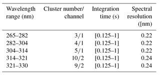
Integration time ranges from 0.125 to 1 s depending on latitude.
In this paper we compare and evaluate the three most recent versions of the SCIAMACHY Level-1 (L1) product. The comparison is based on the retrieval of the nadir ozone profiles from the SCIAMACHY UV reflectance spectra, showing the impact of L1 calibration improvements. The three different L1 data versions used are v7, v7mfac and v8. The primary difference between them is the implementation of degradation correction. These data versions are described in Sect. 2. The result of this paper shows the improved quality of the latest L1 data set version.
The results presented here highlight the need for further corrections of the L1 data. However, a detailed study of radiometric bias corrections in L1 data is beyond the scope of this paper. The focus of this study is to assess the quality of L1 data by analysing the retrieved ozone profiles. We do this for almost the entire mission length of 2003–2011 and we perform validation for the latest version of the L1 data (v8). The Ozone ProfilE Retrieval Algorithm (OPERA) retrieval algorithm is briefly reviewed in Sect. 2.2. Results of the ozone profiles and the comparison between the L1 data sets are shown in Sect. 3. This is followed by comparison to sondes in Sect. 4 for the most recent data set from the years 2003 to 2011. We discuss the possible effects of L1 radiometric bias corrections and applying slit function (SF) corrections in Sect. 5, and finally we conclude in Sect. 6.
SCIAMACHY is a space-borne spectrometer on board ESA's Environmental Satellite Envisat (Burrows et al., 1995; Bovensmann et al., 1999) that was launched in March 2002 and lasted until April 2012. The instrument measures the sunlight reflected by the Earth's atmosphere over a wide spectral range from 212 nm (UV) to 2386 nm (shortwave infrared, SWIR) spread over eight channels. SCIAMACHY can perform measurements in both nadir- and limb-viewing modes (Gottwald and Bovensmann, 2011). These modes usually alternate and the data collected are stored in blocks known as “states”. Each nadir state is essentially an observed area on the Earth's surface, consisting of multiple ground pixels.
The nadir-viewing mode of the instrument corresponds to an instantaneous field of view of 0.045∘ (across track) × 1.8∘ (along track). The observed area is determined by the scan speed of the nadir mirror in the across-track direction, the spacecraft speed in the along-track direction and the integration time (IT). This gives typical ground pixel sizes of 240 km × 30 km corresponding to an IT of 1.0 s and 60 km×30 km for an IT of 0.25 s (Gottwald and Bovensmann, 2011). Typically, a nadir state is an area of (across × along track), consisting of 64 pixels containing the spectra to which ozone profile retrieval algorithm was applied. In order to perform radiometric calibration, SCIAMACHY also observes the Sun once per day.
The L1 data provided to users are generated from raw, uncalibrated Level-0 (L0) data by spectral and radiometric calibration (Lichtenberg et al., 2006). In this paper we retrieve the vertical distribution of ozone using the 265–330 nm L1 data. This wavelength range spreads over channels 1 and 2 of SCIAMACHY, with a partial overlap. We use wavelengths 265–314 nm from Channel 1 and 314–330 nm from Channel 2. The spectrum of each channel is divided into spectral clusters which are groups of wavelengths with a common IT. These spectral clusters, and not the channels, are the organisation structure of the data. The mapping of wavelengths to clusters, the spectral resolution and the IT are listed in Table 1.
The main input quantity for retrieving the ozone profile is the Earth's reflectance spectrum, derived from the L1 product. In this paper the measured reflectance spectrum is defined as
where λ is the wavelength, I is the top-of-atmosphere radiance reflected by the Earth's atmosphere and surface and E is the incident solar irradiance at top-of-atmosphere perpendicular to the solar beam. We note that this definition of reflectance is also called the Sun-normalised radiance. An example of a SCIAMACHY measured reflectance spectrum is shown in Fig. 1 for the spectral range used for the ozone profile retrieval.
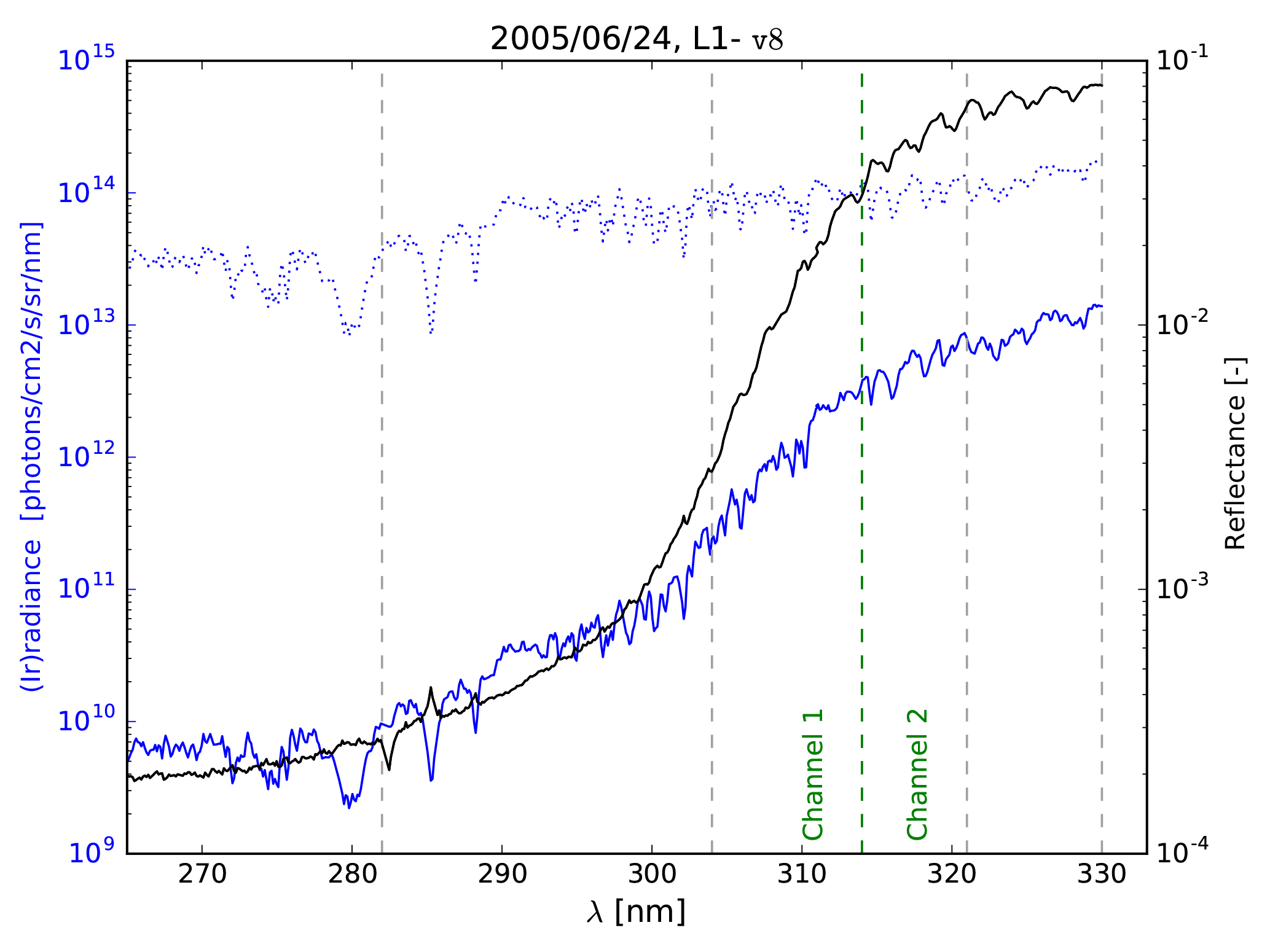
Figure 1Example of SCIAMACHY spectra used for ozone profile retrieval: Earth radiance (solid blue line) and solar irradiance (dotted blue line) in , and reflectance (solid black line) (unit-less). The vertical dashed line in green separates the two channels and the vertical grey lines separate the clusters listed in Table 1.
2.1 Versions of Level-1 data
The uncalibrated L0 data are processed into two sublevels of L1: levels 1b and 1c. The SCIAMACHY specific calibrations applied to the L0 data are described in Slijkhuis et al. (2001). The two sublevels differ in the application of calibration steps: L1c data are processed by full calibration and contains geolocated, spectral radiance and irradiance products. Specifically the calibrated L1c data are produced using ESA's SciaL1C program of v3.2.6. We make use of three different versions of L1c (hereafter called L1) data products described below:
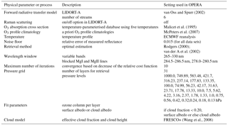
van Oss and Spurr (2002)Malicet et al. (1995)McPeters et al. (2007)Rodgers (2000)van der A et al. (2002)(Wang et al., 2008)Table 2Parameter settings in the OPERA algorithm for SCIAMACHY nadir O3 profile retrieval.
-
v7. This is SCIAMACHY L1 version 7.04−W released in early 2012, where “W” means the processing stage flag and 7.04 is the software version number used for converting L0 into L1 data.
-
v7mfac. This version is identical to the one above, except here we use the degradation correction factors, so-called “m-factors”, that were provided independently as auxiliary data files1. The data structure allows us to turn on and turn off the degradation correction independent of other calibrations. The m-factors are determined by the monitoring of the light path, which is given by the ratio of the measured spectrum of a constant source (Sun) to that obtained for the same optical path at a given time. This gives therefore the degradation of the optical path as the instrument ages. These m-factors are simple multiplication factors to the solar spectrum after the absolute radiometric calibration (Gottwald and Bovensmann, 2011).
-
v8. This is version v8.02, which is the 2016 version of the SCIAMACHY L1 product. The main difference between this version and the one above is the implicit implementation of a standard degradation correction with scan-angle dependence. Specifically the radiometric calibration uses a scan mirror model which takes into account the physical effect of the contamination layers on the mirror. The degradation using this model gives a scan-angle dependence (Bramstedt, 2014).
2.2 OPERA retrieval algorithm
The OPERA, developed in KNMI (van Oss and Spurr, 2002; van der A et al., 2002), retrieves the vertical ozone profile using nadir satellite observations of scattered UV light from the atmosphere. The algorithm makes use of radiative transfer computations of the top-of-atmosphere radiances given the atmospheric scattering and absorption parameters. The ozone absorption cross section decreases from 265 to 330 nm, which allows us to retrieve the amount of ozone as a function of atmospheric height.
In OPERA, the retrieval of ozone profiles uses the maximum a posteriori approach Rodgers (2000). The state of the atmosphere and the measurement are given by the vectors x and y, respectively, and the two vectors are related by the forward model F, according to y=F(x). The solution is given by the following three equations:
where is the retrieved state vector, xa is the a priori, A is the averaging kernel, xt is the “true” state of the atmosphere, is the retrieved covariance matrix, I is the identity matrix, Sa is the a priori covariance matrix, K is the weighting function matrix or Jacobian (which gives the sensitivity of the forward model to the state vector) and Sϵ is the measurement covariance matrix.
The matrices A and provide valuable information on the retrieval. The sum of the diagonal elements of A (i.e. the trace) is called the degrees of freedom for signal (DFS). The higher the DFS, the more the retrieval has learned from the measurement. However, with a low DFS most information in the retrieval is coming from the a priori. The total DFS gives the number of independent pieces of information present in the retrieval. The rows of A are called the smoothing functions, since they give an indication of how xt is smoothed out over the layers of the retrieval. The diagonal elements of the covariance matrix give the variance at the corresponding altitude, while the off-diagonal elements are related to the correlation between the layers in the retrieval. For a comprehensive algorithm overview and retrieval configuration, along with application of the algorithm to GOME-2 data, we refer to Mijling et al. (2010) and van Peet et al. (2014).
The OPERA configuration chosen for application to SCIAMACHY data is given in Table 2. The ozone profile retrieval grid is chosen according to the Nyquist criterion. For SCIAMACHY data we find that setting the retrieval grid to 31 layers or more gives the same value for the DFS. Following van Peet et al. (2014), we have used the McPeters et al. (2007) a priori ozone profiles, because it is a recent climatology (includes ozone depletion) and, unlike other climatologies, it does not require additional parameters like total ozone. Since the McPeters et al. (2007) a priori profiles do not contain covariance matrices, these are assumed to have an exponential decrease in pressure and are scaled with a priori errors (for details see van Peet et al., 2014). OPERA can also use the Fortuin and Kelder (1998) climatology. The reflectance measurement errors are provided in the SCIAMACHY L1 data; a systematic relative error in the measured reflectance (“noise floor”) of 0.015 is added to the measurement errors. The noise floor is assumed the same for all L1 data.
In practice, the measured reflectance spectrum Rmeas(λ) (see Eq. 1) is prepared in the beginning of the OPERA algorithm, which is then passed to the forward model. This model contains vertical atmospheric profiles, like temperature and a priori ozone profile, geolocation, cloud data and surface characteristics. The forward model computes Sun-normalised radiances at the top of the atmosphere at wavelengths determined from the measured instrumental spectral data. After multiplication with a high-resolution solar irradiance reference spectrum and convolution of simulated radiances and irradiances with the instrumental SF, the simulated reflectance spectrum Rsim(λ) is obtained. The inversion step that follows is based on the optimal estimation (OE) method requiring measurement, simulation and measurement errors in vector and matrix forms. An inversion using derivatives of simulated reflectances with respect to the desired parameter to be solved is carried out until convergence is reached or until the maximum number of iterations is reached. For a comprehensive description of the implementation, configuration and the model parameters of the algorithm, we refer to the OPERA manual (Tuinder et al., 2014).
Table 3Statistics of the uncertainties of the L2 ozone profile products that are retrieved using three different versions of L1 data sets (described in Sect. 2.1). This table contains the statistics of the curves shown in Fig. 3.
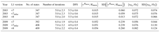
Column 1: L1 data year. Column 2: data set version. Column 3: number of states used. Column 4: median number of iterations ± standard deviation. Column 5: median degrees-of-freedom ± standard deviation. Column 6: median relative uncertainty of converged reflectance spectra in the wavelength band used. Column 7: standard deviation of quantity in Column 6. Column 8: relative uncertainty in retrieved ozone profile. Column 9: standard deviation of quantity in Column 8.
As mentioned above, the averaging kernel (AK) of a retrieval represents the measurement sensitivity with respect to the true state of the atmosphere Rodgers (2000). In Fig. 2 we show an example of the AK for an individual OPERA ozone profile retrieval for a SCIAMACHY state on 7 January 2004. The AK rows represent the smoothing of the true profile as a function of the ozone retrieval layers. These smoothing functions should peak at the corresponding retrieval level and the half-width is a measure for the vertical resolution of the retrieval at that altitude. For an ideal retrieval, the curve of each row will peak at the nominal layer height with a spread that gives the vertical resolution of the retrieval. It is clear from Fig. 2 that information on the ozone amount in a certain layer is also coming from other heights.
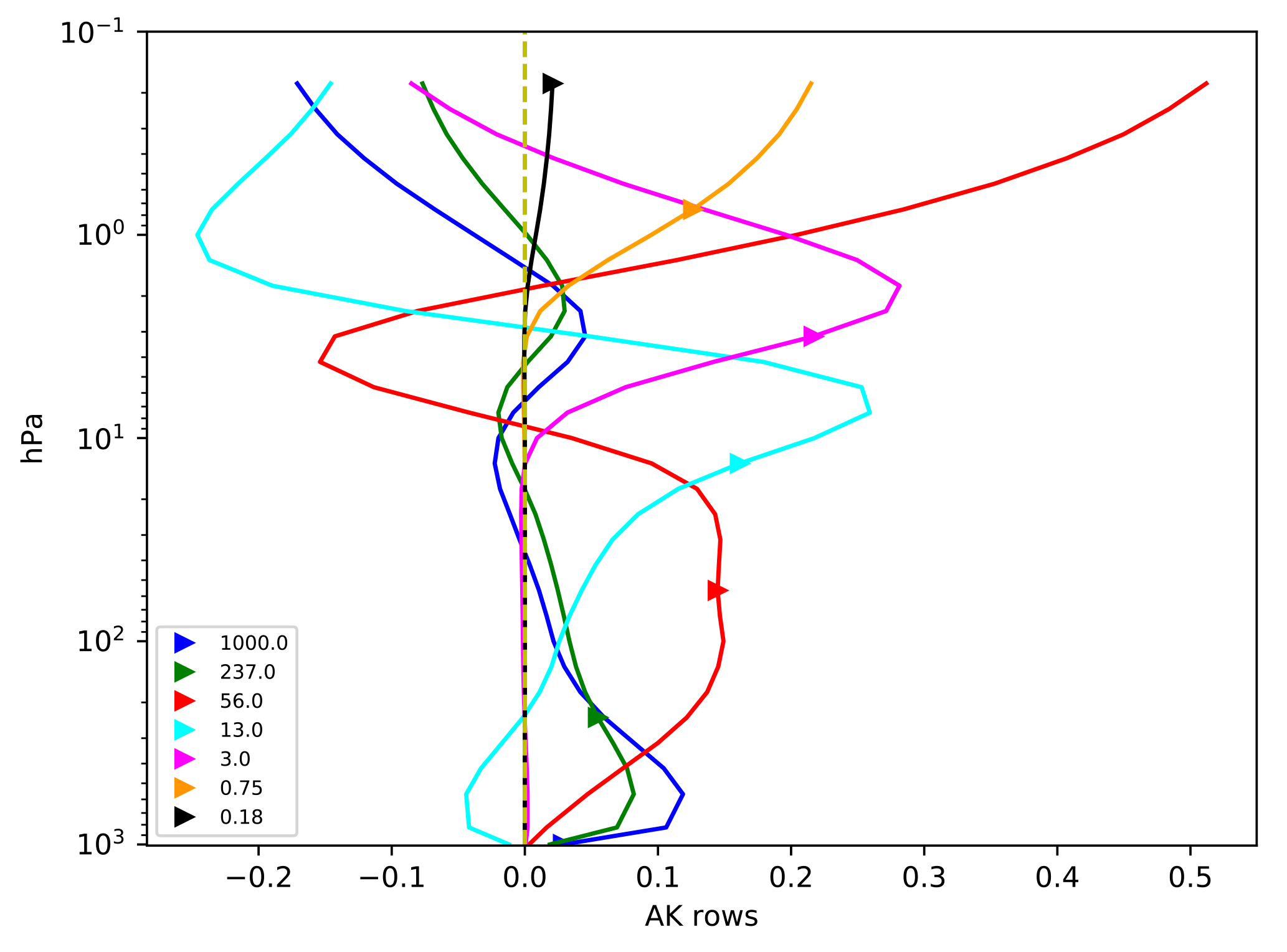
Figure 2Example of the averaging kernel shape for a subset of seven layers from a 31-layer SCIAMACHY ozone profile retrieval. The triangles are the pressure levels in hPa of the retrieval layers. This subset of seven retrieval layers was selected uniformly ranging from top to bottom for clarity.
The aim of this section is to show explicitly the differences in quality between the three different L1 data set versions. This is done by showing the derived Level-2 (L2) product (the vertical ozone profile) in a narrow band in the tropics. Thereto we have performed OPERA retrievals on SCIAMACHY nadir data for almost the entire mission length (2003–2011) for a narrow range of latitudes from 10∘ N to 10∘ S. We have excluded the years 2002 (beginning of the mission) and 2012 (end of the mission) since there are only few months of data in those years. We show the comparison between the L2 products retrieved from the three different L1 data set versions, v7, v7mfac and v8 (described in Sect. 2.1) only for the years 2003 and 2009 below.
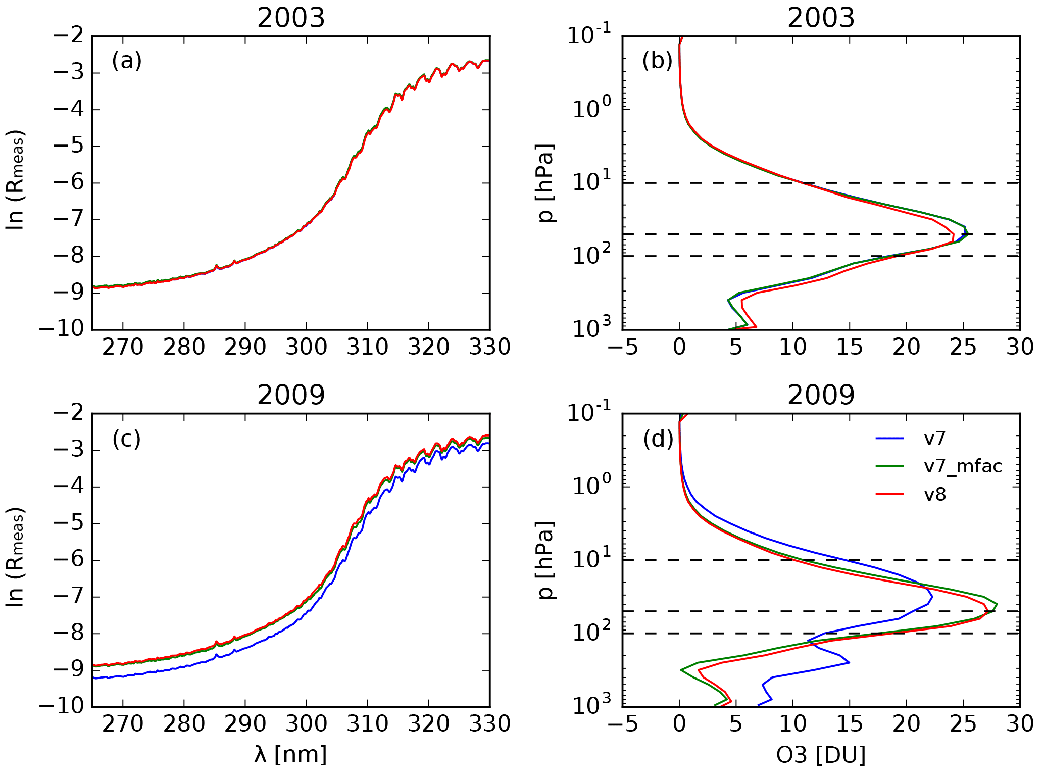
Figure 3(a) Measured reflectance spectra for the year 2003 in natural log units. The spectra are the medians for all states located close to the ozone sonde stations within the tropical latitude band 10∘ N–10∘ S. (b) Corresponding retrieved ozone profiles (in Dobson units per layer) with different colours representing various versions of L1 SCIAMACHY data used. The version 7 with and without degradation correction almost overlap (blue and green lines) whereas version 8 with improved degradation correction has a visible difference in the ozone profile. Panels (c) and (d) are the corresponding figures of panels (a) and (b) for the year 2009. Note the remarkable difference between v7 and later versions with degradation corrections. Here the later two versions almost overlap compared to the case where no degradation is taken into account. The number of states in each data set with corresponding uncertainties are listed in Table 3. The dashed horizontal lines indicates the pressure levels 10, 50 and 100 hPa.
The comparisons are performed for the years 2003 and 2009 to show how the reflectance measurements (and therefore the profiles derived from them) vary from early to late in the SCIAMACHY mission. In Fig. 3 the results for 2003 are shown in the top panels and the results for 2009 are shown in the bottom panels. The left panels show the measured reflectance spectra used by the OPERA retrieval algorithm in estimating the ozone profile shown in the right panels. Each curve is the median of many nadir states: 347 for each data set version of year 2003 and ∼ 400 for the year 2009. The spectrum and ozone profile of each nadir state is the median of all the retrieved pixels of the state, which are typically 65 pixels, sometimes less. The result in the figure is a median for all states over a narrow latitude band in the tropics from 10∘ N to 10∘ S. The different line colours represent different L1 data sets as labelled in the bottom-right panel of the figure. The curves of ozone profiles in the top-right panel for 2003 representing v7 and v7mfac almost overlap each other, showing minimal differences between the two versions; therefore the degradation corrections (m-factors) are also minimal. However, the curve representing v8 in red deviates from the other two visibly, which is hard to see in the reflectance spectra in the left panel. These differences are exacerbated for the year 2009 (later time of the mission), where the ozone profile of v7 is significantly different from v7mfac and v8 in both shape and amount of ozone. The corresponding measured spectra in the bottom-left panel confirm these differences. We also observe visible differences between v7mfac and v8, indicating the intrinsic differences in the implementation of the degradation correction between the two data sets. In the right panels of the figure are horizontal black-dashed lines demarcating the lower-middle stratosphere (100–10 hPa) with another line at 50 hPa. In data set v7 there are large variations in the troposphere (1000–100 hPa) and a significant reduction of the peak of the ozone value in the stratosphere, suggesting the unreliability of this data set for later years of the SCIAMACHY mission. The median errors and standard deviations (SD) along with number of states, number of iterations and DFS statistics of the retrievals of Fig. 3 are listed in Table 3. The maximum number of iterations, n_iter, is set to 10 (see Table 2). The decreasing DFS value going from 2003 to 2009 is further illustrated in Fig. 4, which shows tropical DFS profiles for all months in 2003 and 2009. The DFS profiles for the earlier year (2003) are systematically higher than for the later year (2009). This means that the degradation leads to reduced information content.
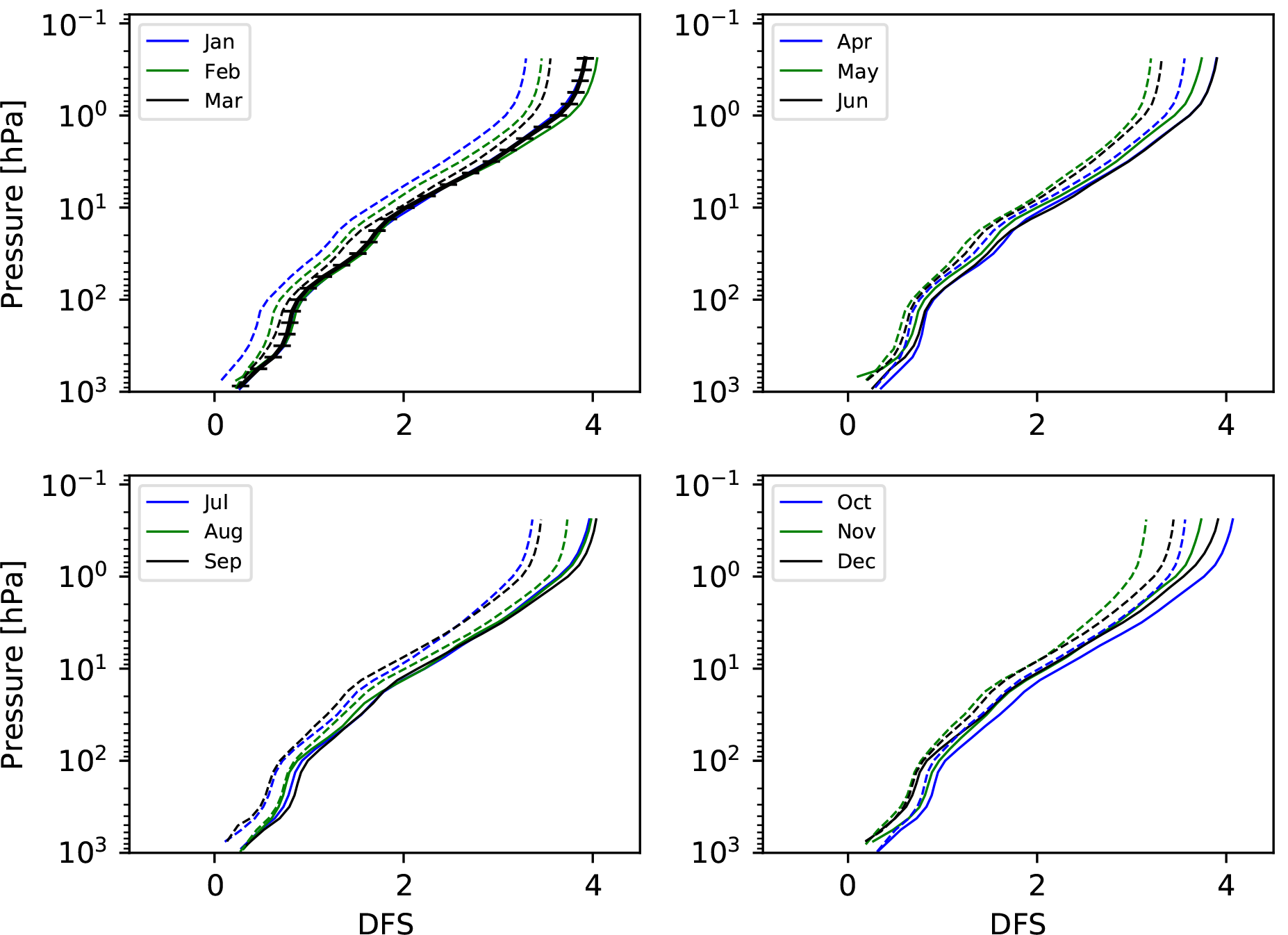
Figure 4Integrated degrees of freedom for signal (DFS) from bottom to each level of SCIAMACHY ozone profile retrievals for individual months for nadir states in the tropics between 15∘ N and 15∘ S. The levels are marked for one of the profiles in the top-left panel with horizontal ticks. The DFS profiles are shown for two years: 2003 in solid lines and 2009 in dashed lines. Here L1 v8 is used.
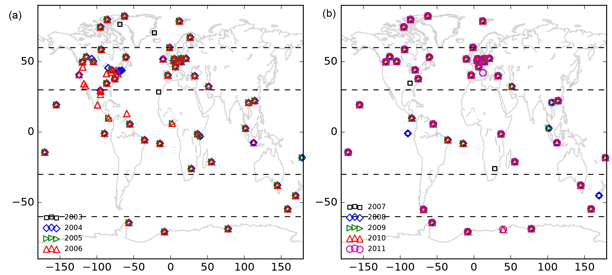
Figure 5Collocated geolocations of satellite data and ozone sonde stations used in the validation. (a) Collocations for years 2003–2006 as labelled. (b) Same for years 2007–2011. Collocations correspond to Fig. 8. The horizontal dashed lines are at 60 and 30∘ N and 30 and 60∘ S.
Table 4Statistics of relative differences between retrieved ozone profiles and ozone sondes for 2003 and 2009, per latitude zone, for the three L1 data versions. All numbers in percent. Bold numbers are exceeding ESA CCI accuracy thresholds.
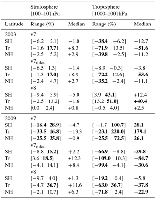
Column 1: Year followed by the latitude zones: Southern Hemisphere (SH), tropics (Tr) and Northern Hemisphere (NH). Column 2: [minimum maximum] of relative differences in the stratosphere for each latitude zone; i.e. minimum corresponds to the minimum deviation in the retrieved sublayers and correspondingly maximum refers to the maximum deviation in the retrieved sublayers. Column 3: medians of relative difference between retrieved and sonde profiles for stratosphere for SH, Tr and NH over the specified altitude range and for the corresponding latitude band. Column 4 and 5: same as Columns 2 and 3, respectively, but for the troposphere.
In this section, we validate SCIAMACHY ozone profile retrievals with ozone sondes with the aim of determining the quality of the three L1 data sets based on external data. We first perform a validation using the three different SCIAMACHY data set versions for 2003 and 2009 in Sect. 4.1, followed by validation using the v8 data set for all the years, 2003–2011 in Sect. 4.2. The aim is to analyse the quality of SCIAMACHY nadir ozone profile retrievals using v7, v7mfac and v8 L1 data. With a UV–VIS instrument it is very hard to retrieve an accurate ozone profile in the troposphere. This is clearly shown in Fig. 4, where the DFS in the troposphere, at pressure levels from ∼ 1000 to 100 hPa, has a maximum value of 1, meaning that there is at most one piece of information in the troposphere. Therefore, we focus the validation on the stratospheric part of the ozone profile between ∼ 100 and 10 hPa.
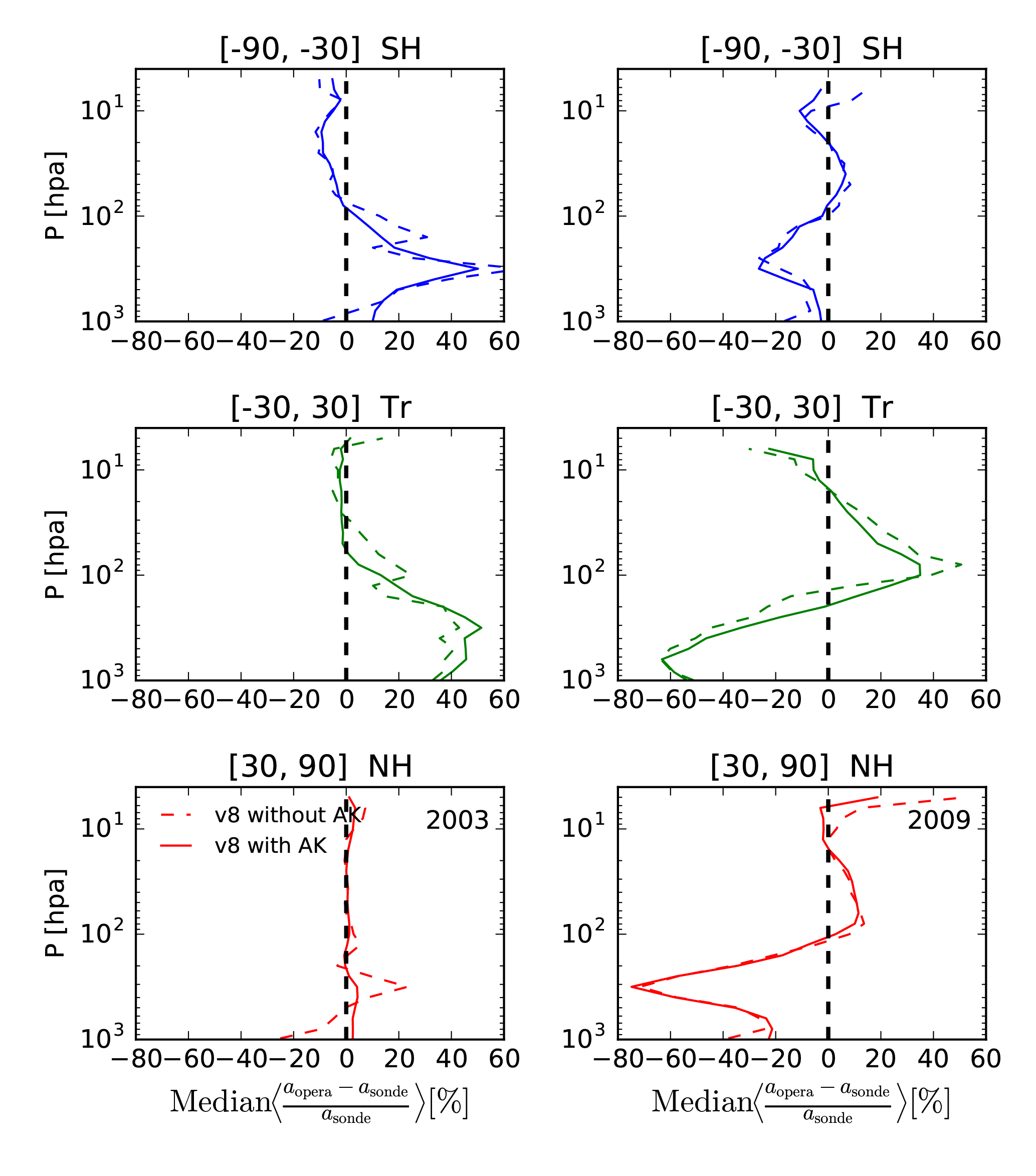
Figure 6Comparison between SCIAMACHY retrieved ozone profiles and ozone sonde profiles with applying averaging kernels (AK, solid lines) and without applying averaging kernels (dashed lines). Here the L1 v8 data set is used for 2003 and 2009.
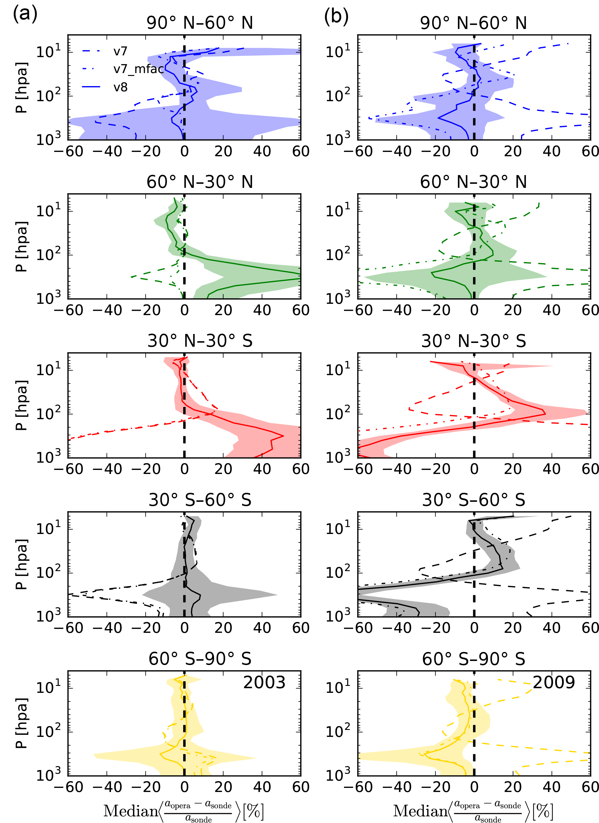
Figure 7Relative difference between ozone profiles retrieved from three different SCIAMACHY L1 data versions and convolved ozone sonde profiles. The three L1 versions are indicated as a dashed line (v7), dash-dotted line (v7mfac) and solid line (v8). The shown quantity is the relative difference in ozone column per layer: (OPERA – sonde)∕sonde. Results are shown in five rows for five latitude bands as indicated. Panel (a) shows results for the year 2003 and panel (b) for the year 2009. The uncertainty band (25–75 percentile difference) in the shaded area is shown for the v8 data set.
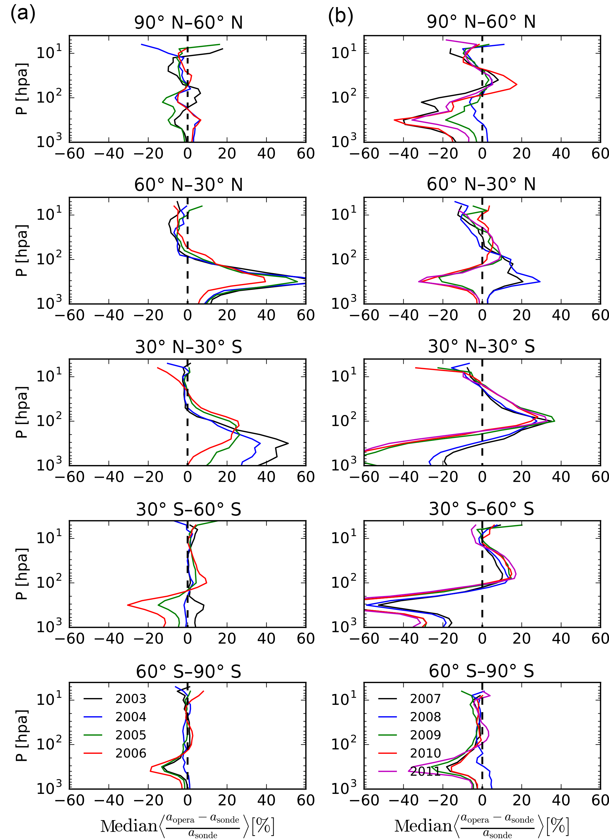
Figure 8Relative difference between ozone profiles retrieved using SCIAMACHY L1 v8 data and convolved ozone sonde profiles, for the period 2003–2011. Results are shown for five latitude bands as indicated. Panel (a) shows results for the years 2003–2006 and panel (b) for the years 2007–2011. Solid lines are median differences of retrieved profiles and sonde profiles [(retrieval – sonde)/sonde] in percent.
For validation, the retrieved ozone profiles are compared with balloon ozone sondes obtained from the World Ozone Ultraviolet Radiation Data Centre (WOUDC, 2011). The sonde is used if it is located within the four corners of the SCIAMACHY state on the ground (the size of which is about 960 km×500 km) and has a measurement date and time within 6 h of the sonde.
The resulting geolocations of the selected sondes are plotted in Fig. 5 for all years. The number of stations for the years 2003–2011 ranges from 38 to 66, with the number of sondes ranging from 1 to 55 per station. The validation algorithm implementing the collocation criteria is similar to the one used by van Peet et al. (2014). We summarise it briefly here and refer to that paper for details.
An ozone sonde profile generally has a higher vertical resolution than a satellite retrieval and can therefore observe more details in the ozone distribution. For the validation the sonde profile should be convolved according to the information present in the AK. The convolved (or smoothed) sonde profile is calculated by convolving the original sonde profile with the AK from the retrieval according to . Above the balloon burst level, the sonde profile is set to the a priori profile before the convolution is calculated. The smoothed sonde profile is then compared to the retrieved profiles from SCIAMACHY. Using a smoothed sonde profile instead of the original sonde profile to compare with the satellite-retrieved profiles influences the results in Figs. 7–8. This is discussed below. To get an impression of the shape of the SCIAMACHY AKs, we refer to Fig. 2.
In Fig. 6, we show the effect on the validation of applying the AK of the satellite retrievals to the ozone sonde profiles for the years 2003 (left panel) and 2009 (right panel). The validation results are clearly less noisy and smoother for the case where the AK was applied to the ozone sondes. For all retrievals presented in this section AK smoothing was used.
4.1 Ozone profile validation comparison between versions v7, v7mfac and v8 for 2003 and 2009
In Fig. 7 we show the ozone profile validation of the three data sets for two years, 2003 and 2009. The results are given for five latitude bands: 90 to 60∘ N, 60 to 30∘ N, 30∘ N to 30∘ S, 30 to 60∘ S and 60 to 90∘ S. For reference, the uncertainties (25–75 % percentiles) in the relative differences are shown only for v8 for all the latitude bands and both years as shaded regions. Each curve is the median difference between retrieved ozone column per layer and the averaging-kernel smoothed ozone sonde value, normalised by the ozone sonde profiles. In the lower-middle stratospheric region a better agreement of the retrieval with the sonde is expected. Qualitatively, it seems that for most latitude regions ozone profiles retrieved from L1 v8 compare better with ozone sondes than profiles retrieved from the earlier L1 versions. For v8 profiles the comparison is generally better in 2003 than in 2009. The quantitative comparison results are given in the following.
The relative differences between the retrieved profiles and the sonde profiles are given in Table 4, where the top half of the table shows the results for the years 2003 and for data sets v7, v7mfac and v8, for three zones: Southern Hemisphere (SH) from 90 to 60∘ S, tropics (Tr) from 30∘ S to 30∘ N, and Northern Hemisphere (NH) from 30 to 90∘ N. In the bottom half of the table these quantities are given for the year 2009. From Table 4 we see that the retrieved profile deviations (median differences in percent) in the stratosphere are systematically smaller than in the troposphere. These large spreads in deviations of satellite retrievals from sondes are also visible in Fig. 7. Any deviation above ∼15 % in the stratosphere and above 20 % in the troposphere are shown in bold numbers for reference, as these are the required accuracy levels in the ESA Ozone CCI project (http://www.esa-ozone-cci.org/). This behaviour is probably not only due to the relatively worsening sensitivity of UV instruments in the troposphere. Rather, it might be due to the limited quality of the SCIAMACHY L1 data. Deviations in retrieved ozone profiles in the upper troposphere and lower stratosphere have been reported due to the ozone variability in a previous study of GOME-2 data (Cai et al., 2012). However, in the stratosphere the median deviations for 2003 are smaller for v8 for Tr and NH compared to the older data set versions, whereas for the SH the three different data sets give comparable deviations. The deviations for 2009 in v8 in the stratosphere are smaller for SH and NH than in the older data sets; the deviations are comparable in the Tr zone between all data sets. Comparison of the ozone profile deviations between 2003 and 2009 show larger values for 2009, suggesting that the quality of L1 v8 data has degraded.
4.2 Validation of v8 ozone profiles for 2003–2011
After establishing the differences between the quality of the three L1 data sets above based on the ozone sondes, here we show the validation results spanning the entire SCIAMACHY observation period using the latest L1 data set. In Fig. 8 we show validation results for the entire data set based on L1 v8 from the years 2003 to 2011, for the same five latitude zones as in Fig. 7. The left column shows results for the earlier years 2003–2006 and the right column for the later years 2007–2011. The solid lines correspond to the difference between satellite and sonde (convolved with satellite AK) normalised by the sonde profile. The number of collocated pixels for all the latitude bands for each year are listed in Table 5 along with median DFS, median number of iterations required to achieve convergence, the median solar zenith angle and the median deviations in percent for each latitude band in the stratosphere and troposphere. From Fig. 8 we note that validation for all latitude bands show in general smaller deviations from the zero line for earlier years than for later years. For later years the agreement with sondes becomes worse especially for tropics and NH bands. The median deviations given in Table 5 show often values higher than 20 % (in boldface) for the troposphere whereas these values are less than 15 % for the stratosphere, deeming them within specifications according to the Ozone CCI requirements (see Sect. 4.1). It should be noted, however, that the large deviations in tropospheric ozone are systematically higher than those for the stratosphere for all zones and the years even for v8, whereas such deviations are not observed for instance with GOME-2 nadir profiles (van Peet et al., 2014).
It can be seen from Fig. 8 that the vertical pattern of differences has changed significantly (and not just the absolute differences) over the instrument lifetime. This is important to consider when applying the profiles for ozone layer studies. This validation of ozone profiles based on L1 v8 suggests that the quality of nadir SCIAMACHY L1 data can still be improved upon. It affects the lowest troposphere in the beginning of the mission and gets worse due to instrument degradation. This is still uncorrected in the UV wavelength range. Please also note the higher deviations in the year 2003 in NH and Tr latitude zones in Fig. 8 as compared to other early years. This is a unique behaviour for 2003; the cause is not clear, but it is probably related to calibration or instrument changes early in the mission. Further improvements are needed (see Sect. 5).
Table 5Validation statistics of retrieved ozone profiles from L1 v8 for the period 2003–2011. Bold numbers in the medians of relative differences are exceeding ESA CCI accuracy thresholds.
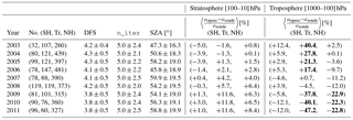
Column 1: Year. Column 2: number of states per latitude zone: Southern Hemisphere (SH), tropics (Tr) and Northern Hemisphere (NH). Column 3: median DFS. Column 4: median number of iterations. Column 5: median solar zenith angle ± standard deviation for all states in that row. Column 6: medians of relative difference between retrieved and sonde profiles for stratosphere for SH, Tr and NH over the specified altitude range and for the corresponding latitude band. Column 7: same as in Column 6 for troposphere.
The deviations found in SCIAMACHY v8 ozone profiles can be compared, for instance, with GOME-2 ozone profile validation by van Peet et al. (2014). Their validation of tropospheric ozone showed deviations ranging from a few percent to ∼ −30 % for the Northern Hemisphere, whereas we find deviations that range from ∼ −10 to −45 % for the year 2008 (blue line in right panels Fig. 8). In the Southern Hemisphere, however, we find the deviations for year 2008 to range from a few percent to ∼ 20 %, which is more comparable to the range of a few percent to found by van Peet et al. (2014).
The accuracy of the retrieved ozone profile is primarily driven by the spectral and radiometric calibration of the measured L1 spectra. In this section we describe two potential L1 corrections that could further improve the quality of the SCIAMACHY L1 spectra: (1) retrieval of the instrumental SF using solar spectra and (2) radiometric bias correction.
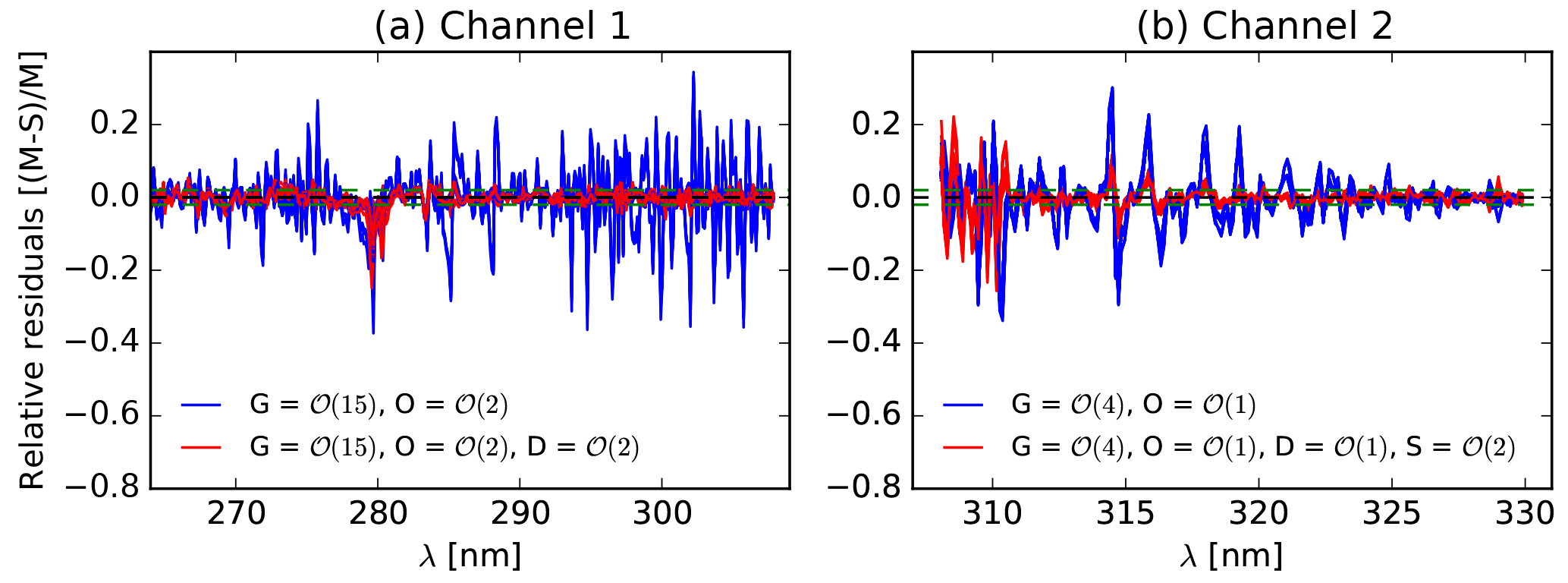
Figure 9Relative residuals of daily SCIAMACHY L1 v8 solar spectra for Channel 1 (a) and Channel 2 (b), found by optimising the slit function parameters O, G, D and S. The residual is defined as , where M is the SCIAMACHY measured irradiance and S is the solar reference spectrum. For visibility, the residuals for only ∼300 spectra are shown, which are representative of the entire mission from August 2002 to April 2012. The dashed lines mark the values of 0 and ±2 %.
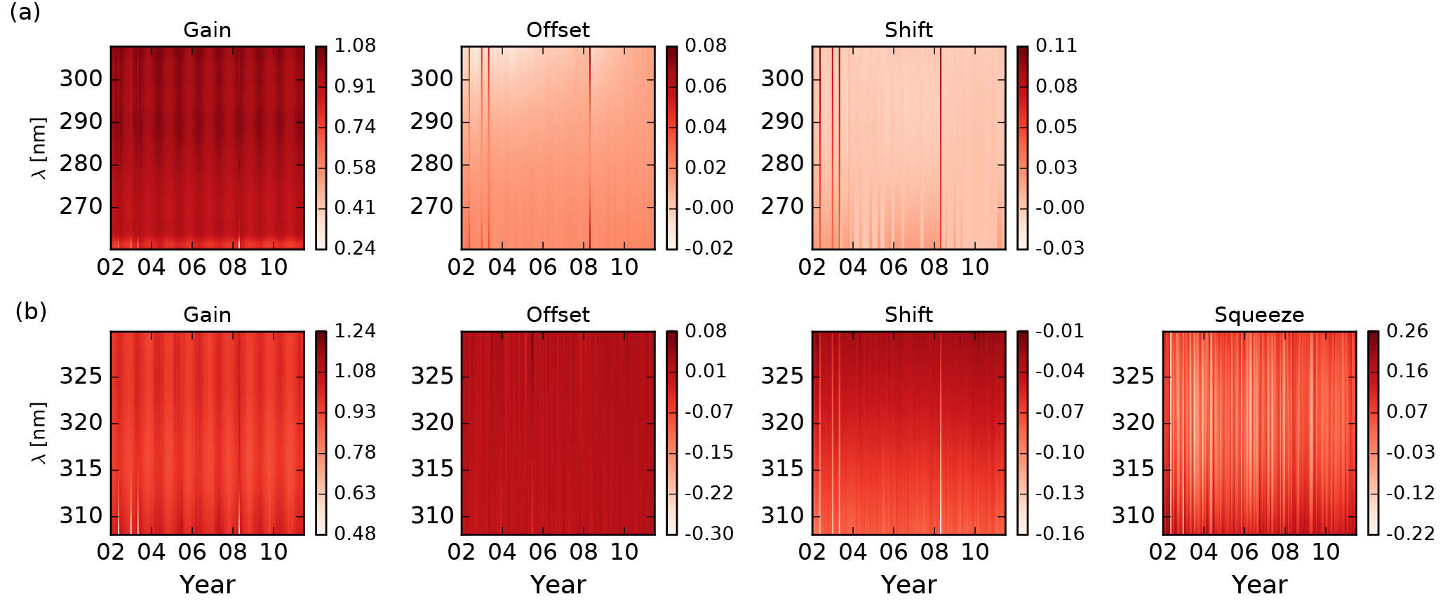
Figure 10Temporal evolution of the slit function parameters for Channel 1 (a) and Channel 2 (b). The time series spans the entire mission for 3466 days, between 2002 and 2012. The ranges of the parameter values are shown to the right to each subplot.
5.1 In-flight slit function calibration using solar measurements
One of the spectral calibrations often performed to assess the behaviour of an instrument in flight is a fit of the instrumental SF (also called instrumental spectral response function). The SF parameters of SCIAMACHY were measured pre-flight and are provided as key data in the L1 product. The slit function S of the instrument has different functional forms depending on the channel. For channels 1–2 (relevant for our ozone profile retrieval) S is described by a single hyperbolic function:
The L1 key data provide the full width half maximum (FWHM), which is related to the a parameter in the equation above. This parameter can be solved in terms of the FWHM by using the fact that at the central point (λ0) we have . Thus, . At each given solar spectrum wavelength, λi, this functional shape is numerically computed between [−1,1] nm centred at λi. This shape can be manipulated with the following four parameters: additive constant (offset, O), multiplication factor (gain, G), displacement of the spectral peak (shift, D) and expansion and contraction of the spectral peak (squeeze, S). The high-resolution solar reference spectrum from Dobber et al. (2008) is modified with these four parameters to best match the SCIAMACHY measured solar irradiance (E(λ)). First the spectral parameters, shift D and squeeze S, are applied to Eq. (5):
followed by the radiometric parameters, gain G and offset O:
The unit of D is nanometre whereas O, G and S are numeric factors. All four parameters depend on wavelength. The parameters FWHM and λ0 at each wavelength, taken from the v8 L1 key data, were identical for all the solar spectra throughout the mission. These values are given at certain wavelengths spread throughout channels 1 and 2 and were interpolated for the wavelengths in-between. An OE algorithm was used to solve for the best parameter values fitting the solar spectrum measurements in flight. The retrieved values of the four parameters at the solar spectrum wavelengths were then also applied to the Earth radiance spectra I(λ) interpolated at the solar spectrum wavelengths.
Thus for each wavelength of the solar spectrum the parameter values are computed using the above SF model. Each spectral peak of the solar reference spectrum can be transformed by manipulating the SF using offset, gain, shift and squeeze until it fits the measured spectrum. These spectral manipulations can be modelled as a polynomial of order n at the desired channels. The fit is checked by evaluating the relative difference between the solar irradiance measurement and simulation, which is the relative residual. The relative residuals for the best fit are shown in Fig. 9. Each curve is a residual for one solar spectrum, where the blue line is achieved by using only gain and offset in the model and the red line is achieved by including the shift and squeeze.
We find that the wavelength range 265–308 nm is the optimal range for obtaining the smallest residuals in Channel 1. However, the ozone profile retrieval algorithm requires spectra from 260 nm onwards. Because the part of Channel 1 above 308 nm is known to suffer of calibration problems, the SF fit in Channel 1 is performed for the range 260–308 nm. We ran the OE on all solar measurements of the SCIAMACHY mission for each day, which amounts to 3463 solar spectra. We convolved all spectra with {offset, gain, shift, squeeze} of polynomial order of = and found that the cost function for the majority of cases reaches less than 1 (as expected) within 10 iterations in the OE routine. By using a spectral shift in the range 265–308 nm instead of in the entire band 265–314 nm the residuals were significantly reduced (see left panel in Fig. 9). No SF fit was possible between 308 and 314 nm. Thus, from 308 nm onwards we used the Channel 2 spectra.
The residuals in Channel 2 are somewhat larger than those in Channel 1 (see Fig. 9). The dashed lines in both panels of the figure mark the ±2 % residuals for reference. Dividing the relevant range of 308–330 nm into smaller ranges to get smaller residuals did not reduce the residuals any further. For the optimal wavelength divisions, we found the smallest residuals given by the polynomial orders of the set of {offset, gain, shift, squeeze} = . In Channel 2, we find that using spectral shift and squeeze in the range 308–330 nm reduces the relative residuals significantly. The relative errors of the L1 solar irradiance in the wavelength range used for ozone profile retrieval, 265–330 nm, are only on the order of 10−5. However, the relative residuals are on the order of a few percent. So we expect this error to propagate into the ozone profile retrieval. There are strong residuals at around 279, 280 and 285 nm due to the MgI and MgII lines in the solar spectra. These spectral windows were therefore not used in the ozone profile retrieval (see Sect. 2).
Figure 10 shows the temporal behaviour of the SF parameters for Channel 1 (Fig. 10a) and Channel 2 (Fig. 10b) as density plots; the fitted parameter value for each wavelength and each day of the year is shown. The seasonal dependence of solar irradiance is observed, as expected, in the gain parameter for both channels. The other parameters do not show a clear seasonal dependence or a clear trend over the mission time.
5.2 Radiometric bias correction
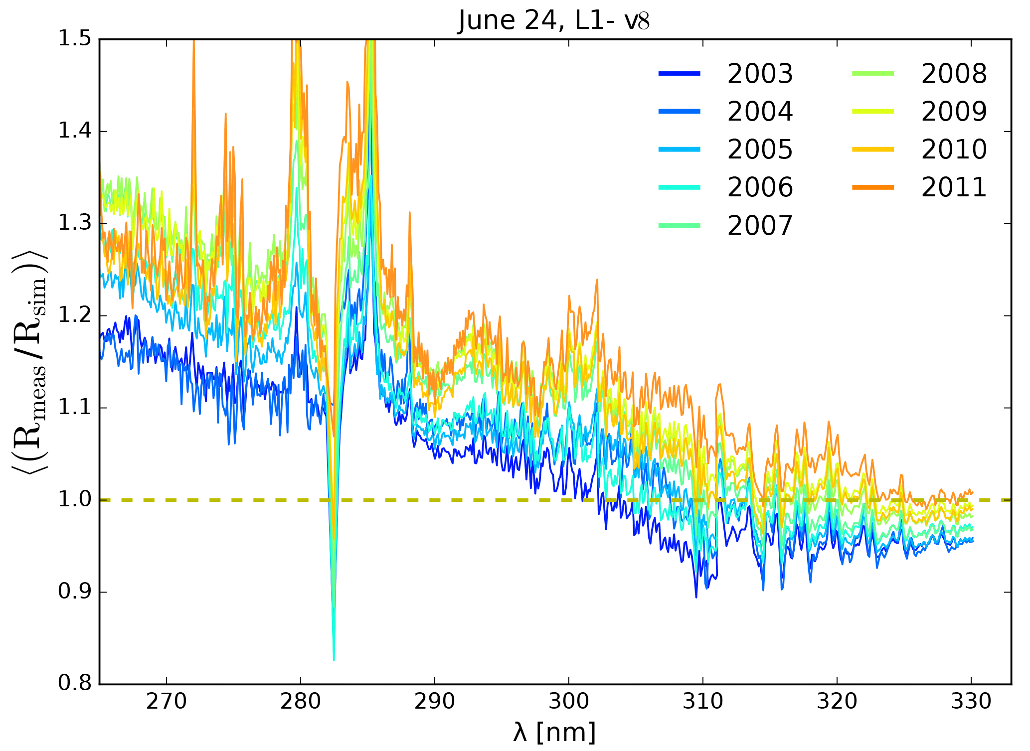
Figure 11Mean ratio of observed (Rmeas) to simulated (Rsim) reflectance spectra for 1 day for each year. The varying rainbow spectrum from blue to red colour labels the ratios for years 2003 to 2011. A horizontal line where the ratio is one is shown for reference.
As shown above, spectral corrections like shift and squeeze at UV wavelengths can further improve the solar spectra by several percent (see Fig. 9). However, the expected improvement from this is less than the degradation and other remaining potential biases for the L1 data, which are increasing with the mission time. A preliminary analysis of this is shown in Fig. 11, where the mean ratio of observed to simulated reflectance spectra (Rmeas∕Rsim) is plotted for the day of 24 June for years 2003–2011. There is a strong deviation of this ratio from one below 300 nm and this becomes worse for later years. A detailed study of this radiometric bias is beyond the scope of this paper. Please note the odd behaviour of the reflectance ratio around 283 nm. This was found to be due to a jump in the value of the Earth radiance at the transition of cluster 3 to cluster 4 owing to the difference in IT. This region is therefore blocked in our retrieval algorithm.
A L1 reflectance bias correction can significantly improve the quality of L1 data and will influence the validation and other results in this paper from their ozone retrievals. Furthermore, applying these bias corrections would also make it meaningful to apply the spectral SF corrections that can potentially improve the ozone retrievals further. Thus a detailed study of the effect of such bias corrections on the L1 data can be investigated against the quality of the ozone retrieval algorithm to better understand the quality of the SCIAMACHY nadir data.
We have performed SCIAMACHY nadir ozone profile retrievals using the OPERA algorithm from three L1 data sets, namely v7, v7mfac and v8. We have used the latest complete data set v8 for almost the entire SCIAMACHY mission length from 2003 to 2011. Differences between L1 data sets with and without degradation corrections (m-factors) were analysed in the wavelength range of 265–330 nm. The resulting L2 ozone profiles from the v8 data set shows vertically smooth profiles for years 2003 and 2009 unlike those for the v7 data set (right panels in Fig. 3). This improved quality is also reflected in the global validation of retrieved ozone profiles against ozone sondes. The comparison between different L1 versions shows that v7 gives significantly worse ozone profiles, especially later in the mission compared to v7mfac and v8, where the profiles of v7 show a double peak for the year 2009 and an overall reduced amount of ozone. Thus L1 v8 should be used for the nadir ozone profile applications of SCIAMACHY data. We have found that further improvement of L1 data is possible. Retrieving the instrument slit function in the UV range for the v8 data set gives an improvement of a few percent in the solar data through the mission length. The measured reflectance spectra show that the degradation in v8 is still significant for some wavelengths, because the ratio of the measured to simulated reflectance below 300 nm can range from ∼ 1.1 to 1.4. This could be corrected empirically by including a bias correction in the L1 data before the ozone profile retrievals
The authors declare that they have no conflict of interest.
The authors would like to thank Gijsbert Tilstra for support with
SCIAMACHY data. The authors would also like to thank all data
contributors to the World Ozone and Ultraviolet Radiation Data Centre (WOUDC)
for submitting their data to a public database and Environment Canada for
hosting the database. ESA and the SCIAMACHY Quality Working Group are
acknowledged for providing and improving the SCIAMACHY L1 data. This work was
funded by the Netherlands Space Office (NSO) through the SCIA-Visie-Extensie
project.
Edited by: Pawan K. Bhartia
Reviewed by: three anonymous referees
Bhartia, P. K., McPeters, R. D., Mateer, C. L., Flynn, L. E., and Wellemeyer, C.: Algorithm for the estimation of vertical ozone pro- files from the backscattered ultraviolet technique, J. Geophys. Res., 101, 18793–18806, https://doi.org/10.1029/96JD01165, 1996. a
Bhartia, P. K., McPeters, R. D., Flynn, L. E., Taylor, S., Kramarova, N. A., Frith, S., Fisher, B., and DeLand, M.: Solar Backscatter UV (SBUV) total ozone and profile algorithm, Atmos. Meas. Tech., 6, 2533–2548, https://doi.org/10.5194/amt-6-2533-2013, 2013. a
Bovensmann, H., Burrows, M. J. P., Buchwitz, M., Frerick, J., Noel, S., Rozanov, V. V., Chance, K. V., and Goede, A. P. H.: SCIAMACHY: Mission objectives and measurement modes, J. Atmos. Sci., 127–150, 1999. a, b
Bramstedt, K.: Scan-angle dependent degradation correction with the scanner model approach, Institute of Environmental Physics (IUP), Doc. No.: IUP-SCIA-TN-Mfactor, University of Bremen, Bremen, Germany, 5–6, 2014. a
Brinksma, E. J., Bracher, A., Lolkema, D. E., Segers, A. J., Boyd, I. S., Bramstedt, K., Claude, H., Godin-Beekmann, S., Hansen, G., Kopp, G., Leblanc, T., McDermid, I. S., Meijer, Y. J., Nakane, H., Parrish, A., von Savigny, C., Stebel, K., Swart, D. P. J., Taha, G., and Piters, A. J. M.: Geophysical validation of SCIAMACHY Limb Ozone Profiles, Atmos. Chem. Phys., 6, 197–209, https://doi.org/10.5194/acp-6-197-2006, 2006. a, b
Burrows, J. P., Holzle, E., Goede, A. P. H., Visser, H., and Fricke, W.: SCIAMACHY – Scanning Imaging Absorption Spectrometer for Atmospheric Chartography, Acta Astronaut., 35, 445–451, 1995. a
Burrows, J. P., Weber, M., Buchwitz, M., Rozanov, V. V., Ladstätter-Weißenmayer, A., Richter, A., de Beek, R., Hoogen, R., Bramstedt, K., Eichmann, K.-U., Eisinger, M., and Perner, D.: The Global Ozone Monitoring Experiment (GOME): Mission concept and first scientific results, J. Atmos. Sci., 56, 151–175, 1999. a
Cai, Z., Liu, Y., Liu, X., Chance, K., Nowlan, C. R., Lang, R., Munro, R., and Suleiman, R.: Characterization and correction of Global Ozone Monitoring Experiment 2 ultraviolet measurements and application to ozone profile retrievals, J. Geophys. Res., 148–227, 2012. a, b
Clerbaux, C., Boynard, A., Clarisse, L., George, M., Hadji-Lazaro, J., Herbin, H., Hurtmans, D., Pommier, M., Razavi, A., Turquety, S., Wespes, C., and Coheur, P.-F.: Monitoring of atmospheric composition using the thermal infrared IASI/MetOp sounder, Atmos. Chem. Phys., 9, 6041–6054, https://doi.org/10.5194/acp-9-6041-2009, 2009. a
Deshler, T., Mercer, J. L., Smit, H. G. J., Stubi, R., Levrat, G., Johnson, B. J., Oltmans, S. J., Kivi, R., Thompson, A. M., Witte, J., Davies, J., Schmidlin, F. J., Brothers, G., and Sasaki, T.: Atmospheric comparison of electrochemical cell ozonesondes from different manufacturers, and with different cathode solution strengths: The Balloon Experiment on Standards for Ozonesondes, J. Geophys. Res., 113, D04307, https://doi.org/10.1029/2007JD008975, 2008. a
Dobber, M., Voors, R., Dirksen, R., Kleipool, Q., and Levelt, P.: The High-Resolution Solar Reference Spectrum between 250 and 550 nm and its Application to Measurements with the Ozone Monitoring Instrument, Sol. Phys., 281–291, 2008. a
ESA: SCIAMACHY Geo-located atmospheric spectra (SCI_NL__1P), available at: https://earth.esa.int/web/guest/data-access/browse-data-products/-/article/sciamachy-localized-atmospheric-spectra-in-the-uvvisnear-ir-wavelength-range-1549, last access: 21 November 2016. a
Fortuin, J. P. F. and Kelder, H.: An ozone climatology based on ozonesonde and satellite measurements, J. Geophys. Res., 103, 31709–31734, 1998. a
Gottwald, M. and Bovensmann, H.: SCIAMACHY – Exploring the Changing Earth's Atmosphere, Springer, Dordrecht, the Netherlands, 225 pp., 2011. a, b, c
Hubert, D., Lambert, J.-C., Verhoelst, T., Granville1, J., Keppens1, A., Baray, J.-L., Bourassa, A. E., Cortesi, U., Degenstein, D. A., Froidevaux, L., Godin-Beekmann, S., Hoppel, K. W., Johnson, B. J., Kyrölä, E., Leblanc1, T., Lichtenberg, G., Marchand, M., McElroy, C. T., Murtagh, D., Nakane, H., Portafaix, T., Querel III, R.,, J. M. R., Salvador, J., Smit, H. G. J., Stebel, K., Steinbrecht, W., Strawbridge, K. B., Stübi, R., Swart, D. P. J., Taha, G., Tarasick, D. W., Thompson, A. M., Urban, J., van Gijsel, J. A. E., Malderen, R. V., von der Gathen, P., Walker, K. A., Wolfram, E., and Zawodny, J. M.: Ground-based assessment of the bias and long-term stability of 14 limb and occultation ozone profile data records, Atmos. Meas. Tech., 9, 2497–2534, https://doi.org/10.5194/amt-9-2497-2016, 2016. a, b
Keppens, A., Lambert, J.-C., Granville, J., Miles, G., Siddans, R., van Peet, J. C. A., van der A, R. J., Hubert, D., Verhoelst, T., Delcloo, A., Godin-Beekmann, S., Kivi, R., Stübi, R., and Zehner, C.: Round-robin evaluation of nadir ozone profile retrievals: methodology and application to MetOp-A GOME-2, Atmos. Meas. Tech., 8, 2093–2120, https://doi.org/10.5194/amt-8-2093-2015, 2015. a
Koelemeijer, R. B. A., de Haan, J. F., and Stammes, P.: A database of spectral surface reflectivity in the range 335–772 nm derived from 5.5 years of GOME observations, J. Geophys. Res.-Atmos., 108, 4070, https://doi.org/10.1029/2002JD002429, 2003.
Kroon, M., de Haan, J. F., Veefkind, J. P., Froidevaux, L., Wang, R., Kivi, R., and Hakkarainen, J. J.: Validation of operational ozone profiles from the Ozone Monitoring Instrument, J. Geophys. Res., 116, D18305, https://doi.org/10.1029/2010JD015100, 2011. a
Levelt, P. F., Hilsenrath, E., Leppelmeier, G. W., van den Oord, G. B. J., Bhartia, P. K., Tamminen, J., de Haan, J. F., and Veefkind, J.: Science objectives of the Ozone Monitoring Instrument, IEEE T. Geosci. Remote Sens., 44, 1199–1208, 2006. a
Lichtenberg, G., Kleipool, Q., Krijger, J. M., van Soest, G., van Hees, R., Tilstra, L. G., Acarreta, J. R., Aben, I., Ahlers, B., Bovensmann, H., Chance, K., Gloudemans, A. M. S., Hoogeveen, R. W. M., Jongma, R. T. N., Noël, S., Piters, A., Schrijver, H., Schrijvers, C., Sioris, C. E., Skupin, J., Slijkhuis, S., Stammes, P., and Wuttke, M.: SCIAMACHY Level 1 data: calibration concept and in-flight calibration, Atmos. Chem. Phys., 6, 5347–5367, https://doi.org/10.5194/acp-6-5347-2006, 2006. a
Liu, X., Bhartia, P. K., Chance, K., Spurr, R. J. D., and Kurosu, T. P.: Ozone profile retrievals from the Ozone Monitoring Instrument, Atmos. Chem. Phys., 10, 2521–2537, https://doi.org/10.5194/acp-10-2521-2010, 2010. a
Malicet, J., Daumont, D., Charbonnier, J., Parisse, C., Chakir, A., and Brion, J.: Ozone UV spectroscopy. II – Absorption crosssections and temperature dependence, J. Atmos. Chem., 21, 263–273, https://doi.org/10.1007/BF00696758, 1995. a
McPeters, R. D., G. J. Labow, and J. A. Logan: Ozone climatological profiles for satellite retrieval algorithms, J. Geophys. Res., 112, D05308, https://doi.org/10.1029/2005JD006823, 2007. a, b, c
Mieruch, S., Weber, M., von Savigny, C., Rozanov, A., Bovensmann, H., Burrows, J. P., Bernath, P. F., Boone, C. D., Froidevaux, L., Gordley, L. L., Mlynczak, M. G., Russell III, J. M., Thomason, L. W., Walker, K. A., and Zawodny, J. M.: Global and long-term comparison of SCIAMACHY limb ozone profiles with correlative satellite data (2002–2008), Atmos. Meas. Tech., 5, 771–788, https://doi.org/10.5194/amt-5-771-2012, 2012. a, b
Mijling, B., Tuinder, O. N. E., van Oss, R. F., and van der A, R. J.: Improving ozone profile retrieval from spaceborne UV backscatter spectrometers using convergence behaviour diagnostics, Atmos. Meas. Tech., 3, 1555–1568, https://doi.org/10.5194/amt-3-1555-2010, 2010. a
Miles, G. M., Siddans, R., Kerridge, B. J., Latter, B. G., and Richards, N. A. D.: Tropospheric ozone and ozone profiles retrieved from GOME-2 and their validation, Atmos. Meas. Tech., 8, 385–398, https://doi.org/10.5194/amt-8-385-2015, 2015. a
Munro, R., Lang, R., Klaes, D., Poli, G., Retscher, C., Lindstrot, R., Huckle, R., Lacan, A., Grzegorski, M., Holdak, A., Kokhanovsky, A., Livschitz, J., and Eisinger, M.: The GOME-2 instrument on the Metop series of satellites: instrument design, calibration, and level 1 data processing – an overview, Atmos. Meas. Tech., 9, 1279–1301, https://doi.org/10.5194/amt-9-1279-2016, 2016. a
Noel, S., Bovensmann, H., Gottwald, M. W. W. J. P. B. M., and Muller, E. K. A. P. H. G. C.: Nadir, limb, and occultation measurements with SCIAMACHY, Adv. Space Res., 29, 1819–1824, 2002.
Rodgers, C. D.: Inverse Methods for Atmospheric Sounding, World Scientific Publishing, Singapore, p. 238, 2000. a, b, c
Slijkhuis, S., Stammes, P., Levelt, P. F., and de Vries, J.: Envisat-1 SCIAMACHY Level 0 to 1c Processing Algorithm Theoretical Basis Document, ENV-ATB-DLR-SCIA-0041, Deutsches Zentrum fuer Luft- und Raumfahrt e.V., Oberpfaffenhofen, Germany, 25–110, 2001. a
Smit, H. G. J., Straeter, W., Johnson, B. J., Oltmans, S. J., Davies, J., Tarasick, D. W., Hoegger, B., Stubi, R., Schmidlin, F. J., Northam, T., Thompson, A. M., Witte, J. C., Boyd, I., and Posny, F.: Assessment of the performance of ECC-ozonesondes under quasi-flight conditions in the environmental simulation chamber: Insights from the Juelich Ozone Sonde Intercomparison Experiment (JOSIE), J. Geophys. Res., 112, 19306, https://doi.org/10.1029/2006JD007308, 2007. a
Staehelin, J.: Global atmospheric ozone monitoring, WMO Bulletin, 57, 45–54, 2008. a
Tuinder, O. N. E., van Oss, R., Mijling, B., and Tilstra, L. G.: OPERA Software User Manual, KNMI-SUM-Manual-2014-01, 2014. a
van der A, R. J., van Oss, R. F., Piters, A. J. M., Fortuin, J. P. F., Meijer, Y. J., and Kelder, H. M.: Ozone profile retrieval from recalibrated Global Ozone Monitoring Experiment data, J. Geophys. Res., 107, 4239, https://doi.org/10.1029/2001JD000696, 2002. a, b
van Oss, R. F. and Spurr, R.: Fast and accurate 4 and 6 stream linearised discrete ordinate radiative transfer models for ozone profile remote sensing retrieval, J. Quant. Spectrosc. Ra., 75, 177–220, 2002. a, b
van Peet, J. C. A., van der A, R. J., Tuinder, O. N. E., Wolfram, E., Salvador, J., Levelt, P. F., and Kelder, H. M.: Ozone ProfilE Retrieval Algorithm (OPERA) for nadir-looking satellite instruments in the UV-VIS, Atmos. Meas. Tech., 7, 859–876, https://doi.org/10.5194/amt-7-859-2014, 2014. a, b, c, d, e, f, g, h
Wang, P., Stammes, P., van der A, R., Pinardi, G., and van Roozendael, M.: FRESCO+: an improved O2 A-band cloud retrieval algorithm for tropospheric trace gas retrievals, Atmos. Chem. Phys., 8, 6565–6576, https://doi.org/10.5194/acp-8-6565-2008, 2008. a
Worden, H. M., Logan, J. A., Worden, J. R., Beer, R., Bowman, K., Clough, S. A., Eldering, A., Fisher, B. M., Gunson, M. R., Herman, R. L., Kulawik, S. S., Lampel, M. C., Luo, M., Megretskaia, I. A., Osterman, G. B., and Shephard, M. W.: Comparisons of Tropospheric Emission Spectrometer (TES) ozone profiles to ozonesondes: Methods and initial results, J. Geophys. Res., 112, D03309, https://doi.org/10.1029/2006JD007258, 2007. a
ozone holewas discovered in the 1980s. We study and assess the quality of the ozone profiles using SCIAMACHY ultraviolet data and compare them against the ozone sondes.