the Creative Commons Attribution 4.0 License.
the Creative Commons Attribution 4.0 License.
 | 26 Apr 2018
Algorithm theoretical baseline for formaldehyde retrievals from S5P TROPOMI and from the QA4ECV project
Isabelle De Smedt
Nicolas Theys
Huan Yu
Thomas Danckaert
Christophe Lerot
Steven Compernolle
Michel Van Roozendael
Andreas Richter
Andreas Hilboll
Enno Peters
Mattia Pedergnana
Diego Loyola
Steffen Beirle
Thomas Wagner
Henk Eskes
Jos van Geffen
Klaas Folkert Boersma
Pepijn Veefkind
On board the Copernicus Sentinel-5 Precursor (S5P) platform, the TROPOspheric Monitoring Instrument (TROPOMI) is a double-channel, nadir-viewing grating spectrometer measuring solar back-scattered earthshine radiances in the ultraviolet, visible, near-infrared, and shortwave infrared with global daily coverage. In the ultraviolet range, its spectral resolution and radiometric performance are equivalent to those of its predecessor OMI, but its horizontal resolution at true nadir is improved by an order of magnitude. This paper introduces the formaldehyde (HCHO) tropospheric vertical column retrieval algorithm implemented in the S5P operational processor and comprehensively describes its various retrieval steps. Furthermore, algorithmic improvements developed in the framework of the EU FP7-project QA4ECV are described for future updates of the processor. Detailed error estimates are discussed in the light of Copernicus user requirements and needs for validation are highlighted. Finally, verification results based on the application of the algorithm to OMI measurements are presented, demonstrating the performances expected for TROPOMI.


Long-term satellite observations of tropospheric formaldehyde (HCHO)1 are essential to support studies related to air quality and chemistry–climate from the regional to the global scale. Formaldehyde is an intermediate gas in almost all oxidation chains of non-methane volatile organic compounds (NMVOCs), leading eventually to CO2 (Seinfeld and Pandis, 2006). NMVOCs are, together with NOx, CO, and CH4, among the most important precursors of tropospheric ozone. NMVOCs also produce secondary organic aerosols and influence the concentrations of OH, the main tropospheric oxidant (Hartmann et al., 2013). The major HCHO source in the remote atmosphere is CH4 oxidation. Over the continents, the oxidation of higher NMVOCs emitted from vegetation, fires, traffic, and industrial sources results in important and localized enhancements of the HCHO levels (as illustrated in Fig. 1; Stavrakou et al., 2009a). With its lifetime of the order of a few hours, HCHO concentrations in the boundary layer can be related to the release of short-lived hydrocarbons, which mostly cannot be observed directly from space. Furthermore, HCHO observations provide information on the chemical oxidation processes in the atmosphere, including CO chemical production from CH4 and NMVOCs. The seasonal and interannual variations of the formaldehyde distribution are principally related to temperature changes (controlling vegetation emissions) and fire events, but also to changes in anthropogenic activities (Stavrakou et al., 2009b). For all these reasons, HCHO satellite observations are used in combination with tropospheric chemistry transport models to constrain NMVOC emission inventories in so-called top-down inversion approaches (e.g. Abbot et al., 2003; Palmer et al., 2006; Fu et al., 2007; Millet et al., 2008; Stavrakou et al., 2009a, b, 2014, 2015; Curci et al., 2010; Barkley et al., 2011, 2013: Fortems-Cheiney et al., 2012; Marais et al., 2012; Mahajan et al., 2015; Kaiser et al., 2017).
HCHO tropospheric columns have been successively retrieved from GOME on ERS-2 and from SCIAMACHY on ENVISAT, resulting in a continuous dataset covering a period of almost 16 years from 1996 until 2012 (Chance et al., 2000; Palmer et al., 2001; Wittrock et al., 2006; Marbach et al., 2009; De Smedt et al., 2008, 2010). Starting in 2007, the measurements made by the three GOME-2 instruments (EUMETSAT Metop A, B, and C) have the potential to extend by more than a decade the successful time series of global formaldehyde morning observations (Vrekoussis et al., 2010; De Smedt et al., 2012; Hewson et al., 2013; Hassinen et al., 2016). Since its launch in 2004, OMI on the NASA AURA platform has been providing complementary HCHO measurements in the early afternoon with daily global coverage and a better spatial resolution than current morning sensors (Kurosu, 2008; Millet et al., 2008; González Abad et al., 2015; De Smedt et al., 2015). On the S-NPP spacecraft, OMPS has also allowed the retrieval of HCHO columns since the end of 2011 (Li et al., 2015; González Abad et al., 2016). TROPOMI aims to continue this time series of early afternoon observations, with daily global coverage, a spectral resolution, and signal-to-noise ratio (SNR) equivalent to OMI, but combined with a spatial resolution improved by an order of magnitude, which potentially offers an unprecedented view of the spatiotemporal variability of NMVOC emissions (Veefkind et al., 2012).
To fully exploit the potential of satellite data, applications relying on tropospheric HCHO observations require high-quality, long-term time series, provided with well-characterized errors and averaging kernels, and consistently retrieved from the different sensors. Furthermore, as the HCHO observations are aimed to be used synergistically with other species observations (e.g. with NO2 for air quality applications), it is essential to homogenize the retrieval methods as well as the external databases as much as possible in order to minimize systematic biases between the observations. The design of the TROPOMI HCHO prototype algorithm, developed at BIRA-IASB, has been driven by the experience developed with formaldehyde retrievals from the series of precursor missions OMI, GOME(-2), and SCIAMACHY. Furthermore, within the Sentinel-5 Precursor (S5P) Level 2 Working Group project (L2WG), a strong component of verification has been developed involving independent retrieval algorithms for each operational prototype algorithm. For HCHO, the University of Bremen (IUP-UB) has been responsible of the algorithm verification. An extensive comparison of the processing chains of the prototype (the retrieval algorithm presented in this paper) and verification algorithm has been conducted. In parallel, within the EU FP7-project Quality Assurance for Essential Climate Variables (QA4ECV; Lorente et al., 2017), a detailed step-by-step study has been performed for HCHO and NO2 differential optical absorption spectroscopy (DOAS) retrievals, including more scientific algorithms (BIRA-IASB, IUP-UB, MPIC, KNMI, and WUR), leading to state-of-the-art European products (http://www.qa4ecv.eu). Those iterative processes led to improvements that have been included in the S5P prototype algorithm or have been proposed as options for future improvements of the operational algorithm.

Figure 1Ten-year average of HCHO vertical columns retrieved from OMI between 2005 and 2014 (http://www.qa4ecv.eu/ecv/hcho-p/data).
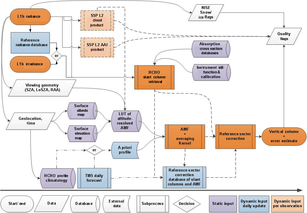
Figure 2Flow diagram of the L2 HCHO retrieval algorithm implemented in the S5P operational processor.
This paper gives a thorough description of the TROPOMI HCHO algorithm baseline, as implemented at the German Aerospace Center (DLR) in the S5P operational processor UPAS-2 (Universal Processor for UV/VIS Atmospheric Spectrometers). It reflects the S5P HCHO Level 2 (L2) Algorithm Theoretical Basis Document v1.0 (De Smedt et al., 2016) and also describes the options to be activated after the S5P launch, as implemented for the QA4ECV OMI HCHO retrieval algorithm (see illustration in Fig. 1).
In Sect. 2, we discuss the product requirements and the expected product performance in terms of precision and trueness and provide a complete description of the retrieval algorithm. In Sect. 3, the uncertainty of the retrieved columns and the error budget is presented. Results from the algorithm verification exercise are given in Sect. 4. The possibilities and needs for future validation of the retrieved HCHO data product can be found in Sect. 5. Conclusions are given in Sect. 6.
2.1 Product requirements
In the UV, the sensitivity to HCHO concentrations in the boundary layer is intrinsically limited from space due to the combined effect of Rayleigh and Mie scattering that limits the fraction of radiation scattered back from low altitudes and reflected from the surface to the satellite. In addition, ozone absorption reduces the number of photons that reach the lowest atmospheric layers. Furthermore, the absorption signatures of HCHO are weaker than those of other UV–visible absorbers, such as NO2. As a result, the retrieval of formaldehyde from space is sensitive to noise and prone to error. While the precision (or random uncertainty) is mainly driven by the SNR of the recorded spectra, the trueness (or systematic uncertainty) is limited by the current knowledge on the external parameters needed in the different retrieval steps.
The requirements for HCHO retrievals have been identified as part of “Science Requirements Document for TROPOMI” (van Weele et al., 2008), the “GMES Sentinels 4 and 5 Mission Requirements Document” (Langen et al., 2011, 2017), and the S5P Mission Advisory Group “Report of the Review of User Requirements for Sentinels-4/-5” (Bovensmann et al., 2011). The requirements for HCHO are summarized in Table 1. Uncertainty requirements include retrieval and measurement (instrument-related) errors. Absolute requirements (in total column units) relate to background conditions, while percentage values relate to elevated columns.
Table 1Requirements on HCHO vertical tropospheric column products as derived from the COPERNICUS Sentinels 4 and 5 Mission Requirements Document. Where numbers are given as a range, the first is the target requirement and the second is the threshold requirement.
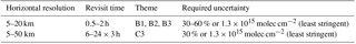
Three main COPERNICUS environmental themes have been defined as ozone layer (A), air quality (B), and climate (C) with further division into sub-themes. Requirements for HCHO have been specified for a number of these sub-themes (B1: Air Quality Protocol Monitoring; B2: Air Quality Near-Real Time; B3: Air Quality Assessment; and C3: Climate Assessment). With respect to air quality protocol monitoring, which is mostly concerned with trend and variability analysis, the requirements are specified for NMVOC emissions on monthly to annual timescales and on larger regional and country scales (Bovensmann et al., 2011). In the error analysis section, we discuss these requirements and the expected performances of the HCHO retrieval algorithm.

Figure 3Example of regional and monthly averages of the HCHO vertical columns over different NMVOC emission regions, derived from OMI observations for the period 2005–2014. Results of the retrievals in the two fitting intervals (1: 328.5–359 nm and 2: 328.5–346 nm, with BrO fitted in interval 1) are shown, as well as the magnitude of the background vertical column (Nv,0).
2.2 Algorithm description
Figure 2 displays a flow diagram of the L2 HCHO retrieval algorithm implemented in the S5P operational processor. The baseline operation flow scheme is based on the DOAS retrieval method (Platt, 1994; Platt and Stutz, 2008; and references therein). It is identical in concept to the retrieval method of SO2 (Theys et al., 2017) and very close to that of NO2 (van Geffen et al., 2017). The interdependencies with auxiliary data and other L2 retrievals, such as clouds, aerosols, or surface reflectance, are also represented.
Following the diagram in Fig. 2, the processing of S5P Level 1b (L1b) data proceeds as follows: radiance and irradiance spectra are read from the L1b file, along with geolocation data such as pixel coordinates and observation geometry (sun and viewing angles). The relevant absorption cross-section data and characteristics of the instrument are used as input for the determination of the HCHO slant columns (Ns). In parallel to the slant column fit, S5P cloud information and absorbing aerosol index (AAI) data are obtained from the operational chain. Additionally, in order to convert the slant column to a vertical column (Nv), an air mass factor (AMF) that accounts for the average light path through the atmosphere is calculated. For this purpose, several auxiliary data are read from external (operational and static) sources: cloud cover data, topographic information, surface albedo, and the a priori shape of the vertical HCHO profile in the atmosphere. The AMF is computed by combining an a priori formaldehyde vertical profile and altitude-resolved AMFs extracted from a pre-computed look-up table (LUT; also used as a basis for the error calculation and retrieval characterization module). This LUT has been created using the VLIDORT 2.6 radiative transfer model (Spurr et al., 2008a) at a single wavelength representative of the retrieval interval. It is used to compute the total column averaging kernels (Eskes and Boersma, 2003), which provide essential information on the measurement vertical sensitivity and are required for comparison with other types of data.
Background normalization of the slant columns is required in the case of weak absorbers such as formaldehyde. Before converting the slant columns into vertical columns, background values of Ns are normalized to compensate for possible systematic offsets (reference sector correction, see below). The tropospheric vertical column end product results therefore from a differential column to which the HCHO background is added due to methane oxidation, estimated using a tropospheric chemistry transport model.
The final tropospheric HCHO vertical column is obtained using the following equation:
The main outputs of the algorithm are the slant column density (Ns), the tropospheric vertical column (Nv), the tropospheric air mass factor (M), and the values used for the reference sector correction (Ns,0 and Nv,0). Complementary product information includes the clear-sky air mass factor, the uncertainty on the total column, the averaging kernel, and quality flags. Table 13 in Appendix B gives a non-exhaustive set of data fields that are provided in the L2 data product. A complete description of the L2 data format is given in the S5P HCHO Product User Manual (Pedergnana et al., 2017).
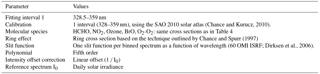
Table 2Summary of algorithm settings used to retrieve HCHO tropospheric columns from TROPOMI spectra. The last column lists additional features implemented in the QA4ECV HCHO product, which are options for future updates of the S5P Processor.
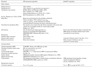
Algorithmic steps are described in more detail in the next sections, and settings are summarized in Table 2, along with algorithmic improvements developed in the framework of the EU FP7-project QA4ECV and proposed for future TROPOMI processor updates. Figure 3 presents examples of monthly averaged HCHO vertical columns over four NMVOC emission regions, along with the background correction values.
2.2.1 Formaldehyde slant column retrieval
The DOAS method relies on the application of the Beer–Lambert law. The backscattered earthshine spectrum as measured by the satellite spectrometer contains the strong solar Fraunhofer lines and additional fainter features due to interactions taking place in the Earth atmosphere during the incoming and outgoing paths of the radiation. The basic idea of the DOAS method is to separate broad and narrowband spectral structures of the absorption spectra in order to isolate the narrow trace gas absorption features. In practice, the application of the DOAS approach to scattered light observations relies on the following key approximations.
For weak absorbers the exponential function can be linearized and the Beer–Lambert law can be applied to the measured radiance to which a large variety of atmospheric light paths contributes.
The absorption cross sections are assumed to be weakly dependent on temperature and independent of pressure. This allows the expression of light attenuation in terms of the Beer–Lambert law and (together with approximation 1) separating spectroscopic retrievals from radiative transfer calculations by introducing the concept of one effective slant column density for the considered wavelength window.
Broadband variations are approximated by a common low-order polynomial to compensate for the effects of loss and gain from scattering and reflections by clouds and air molecules and/or at the Earth surface.
The DOAS equation is obtained by considering the logarithm of the radiance I(λ) and the irradiance E0(λ) (or another reference radiance selected in a remote sector) and including all broadband variations in a polynomial function:
where the measured optical depth is modelled using a highly structured part and a broadband variation .
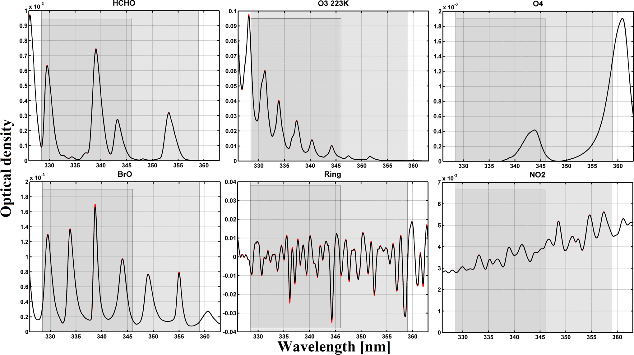
Figure 4Typical optical densities of HCHO, O3, O2-O2, BrO, Ring effect, and NO2 in the near UV. The slant columns have been taken as 1.3 × 10¹⁶ molec cm−2 for HCHO, 1019 molec cm−2 for O3, 0.4 × 1043 molec2 cm−5 for O2-O2, 1014 molec cm−2 for BrO, and 1 × 10¹⁶ molec cm−2 for NO2. A ratio of 8 % has been taken for Raman scattering (Ring effect). High-resolution absorption cross sections of Table 2 have been convolved with the TROPOMI ISFR v1.0 (row 1 is shown in red and row 225 in black; see also Fig. 5). The two fitting intervals (−1 and −2) used to retrieve HCHO slant columns are limited by grey areas.
Equation (2) is a linear equation between the logarithm of the measured quantities (I and E0), the slant column densities of all relevant absorbers (Ns,j), and the polynomial coefficients (cp), at multiple wavelengths. DOAS retrievals consist in solving an overdetermined set of linear equations, which can be done by standard methods of linear least-squares fit (Platt and Stutz, 2008). The fitting process consists in minimizing the chi-square function, i.e. the weighted sum of squares derived from Eq. (3):
where the summation is made over the individual spectral pixels included in the selected wavelength range (k is the number of spectral pixels in the fitting interval). εi is the statistical uncertainty on the measurement at wavelength λi. Weighting the residuals by the instrumental errors εi is optional. When no measurement uncertainties are used (or no error estimates are available), all uncertainties in Eq. (4) are set to εi=1, giving all measurement points equal weight in the fit.
In order to optimize the fitting procedure, additional structured spectral effects have to be considered carefully such as the Ring effect (Grainger and Ring, 1962). Furthermore, the linearity of Eq. (3) may be broken down by instrumental aspects such as small wavelength shifts between I and E0.
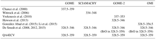
Table 3Wavelength intervals used in previous formaldehyde retrieval studies (nm).
Fitting intervals, absorption cross sections, and spectral fitting settings
Despite the relatively large abundance of formaldehyde in the atmosphere (of the order of 1016 molec cm−2) and its well-defined absorption bands, the fitting of HCHO slant columns in earthshine radiances is a challenge because of the low optical density of HCHO compared to other UV–visible absorbers. The typical HCHO optical density is 1 order of magnitude smaller than that of NO2 and 3 orders of magnitude smaller than that for O3 (see Fig. 4). Therefore, the detection of HCHO is limited by the SNR of the measured radiance spectra and by possible spectral interferences and misfits due to other molecules absorbing in the same fitting interval, mainly ozone, BrO, and O4. In general, the correlation between cross sections decreases when the wavelength interval is extended, but the assumption of a single effective light path defined for the entire wavelength interval may not be fully satisfied, leading to systematic misfit effects that may also introduce biases in the retrieved slant columns. To optimize DOAS retrieval settings, a trade-off has to be found minimizing these effects taking also into consideration the instrumental characteristics. A basic limitation of the classical DOAS technique is the assumption that the atmosphere is optically thin in the wavelength region of interest. At shorter wavelengths, the usable spectral range of DOAS is limited by rapidly increasing Rayleigh scattering and O3 absorption. The DOAS assumptions start to fail for ozone slant columns larger than 1500 DU (Van Roozendael et al., 2012). Historically, different wavelength intervals have been selected between 325 and 360 nm for the retrieval of HCHO using previous satellite UV spectrometers (e.g. GOME, Chance et al., 2000; SCIAMACHY, Wittrock et al., 2006; or GOME-2, Vrekoussis et al., 2010). The TEMIS dataset combines HCHO observations from GOME, SCIAMACHY, GOME-2, and OMI measurements retrieved in the same interval (De Smedt et al., 2008, 2012, 2015). The NASA operational and PCA OMI algorithm exploit a larger interval (Kurosu, 2008; González Abad et al., 2015; Li et al., 2015). The latest QA4ECV product uses the largest interval, thanks to the good quality of the OMI level 1 spectra. A summary of the different wavelength intervals is provided in Table 3.
As for the TEMIS OMI HCHO product (De Smedt et al., 2015), the TROPOMI L2 HCHO retrieval algorithm includes a two-step DOAS retrieval approach, based on two wavelength intervals.
-
328.5–359 nm: This interval includes six BrO absorption bands and minimizes the correlation with HCHO, allowing a significant reduction of the retrieved slant column noise. Note that this interval includes part of a strong O4 absorption band around 360 nm, which may introduce geophysical artefacts of HCHO columns over arid soils or high-altitude regions.
-
328.5–346 nm: in a second step, HCHO columns are retrieved in a shorter interval, but using the BrO slant column values determined in the first step. This approach allows us to efficiently decorrelate BrO from HCHO absorption while, at the same time, the O4-related bias is avoided.
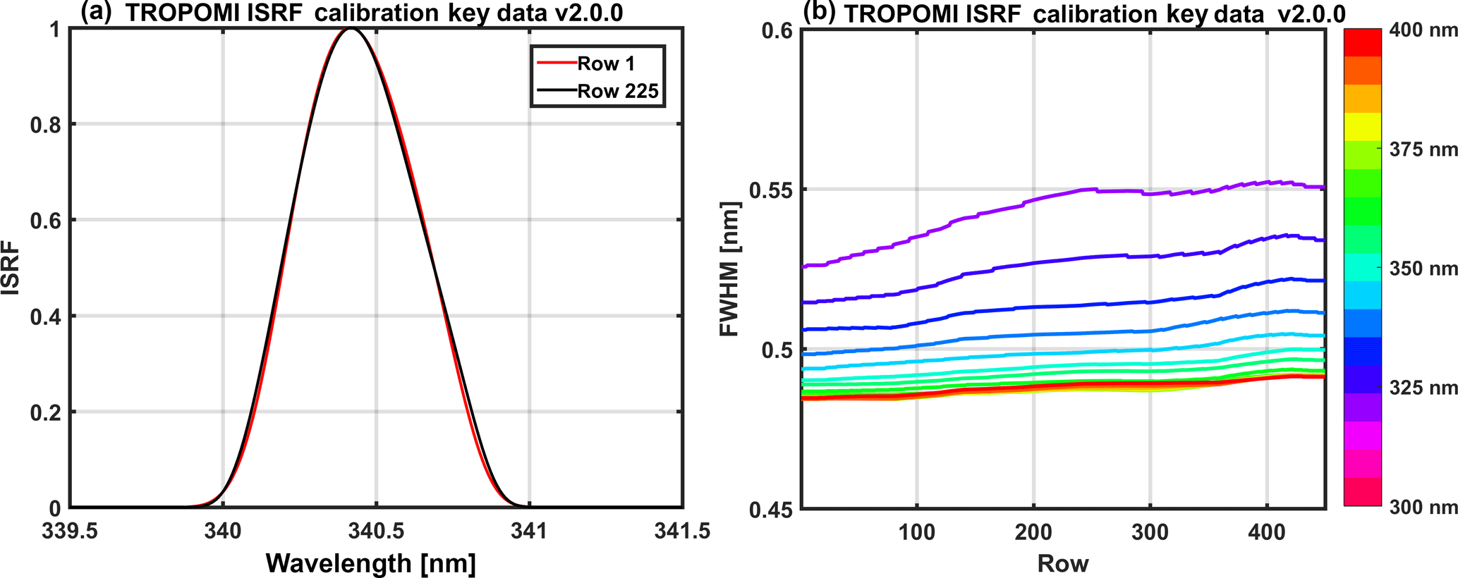
Figure 5(a) Examples of TROPOMI slit functions around 340 nm, for row 1 and row 225. (b) TROPOMI spectral resolution in channel 3, as a function of the row and the wavelength, derived from the instrument key data ISFR v2.0.0.
The use of a large fitting interval generally allows for a reduction of the noise on the retrieved slant columns. However, a substantial gain can only be obtained if the L1b spectra are of sufficiently homogeneous quality over the full spectral range. Indeed, experience with past sensors not equipped with polarization scramblers (e.g. GOME(-2) or SCIAMACHY) has shown that this gain can be partly or totally overruled due to the impact of interfering spectral polarization structures (De Smedt et al., 2012, 2015). Assuming spectra free of spectral features, the QA4ECV baseline option using one single large interval (fitting interval 1) will be applicable to TROPOMI in order to further improve the precision. Results of the retrievals from the two intervals applied to OMI are presented in Fig. 3. In this case, vertical column differences between the two intervals are generally lower than 10 %. They can, however, reach 20 % in wintertime.
In both intervals, the absorption cross sections of O3 at 223 and 243 K, NO2, BrO, and O4 are included in the fit. The correction for the Ring effect, defined as Irrs∕Ielas, where Irrs and Ielas are the intensities for inelastic (rrs: rotational Raman scattering) and elastic scattering processes, is based on the technique published by Chance and Spurr (1997). Furthermore, in order to better cope with the strong ozone absorption at wavelengths shorter than 336 nm, the method of Puķīte et al. (2010) is implemented. In this method, the variation of the ozone slant column over the fitting window is taken into account. On the first order, the method consists in adding two cross sections to the fit: and (Puķīte et al., 2010; De Smedt et al., 2012), using the O3 cross sections at 223 K (close to the temperature at ozone maximum in the tropics). It allows a much better treatment of optically thick ozone absorption in the retrieval and therefore to reduce the systematic underestimation of the HCHO slant columns by 50 to 80 %, for solar zenith angle (SZA) from 50 to 70∘.
To obtain the optical density (Eq. 2), the baseline option is to use the daily solar irradiance. A more advanced option, implemented in QA4ECV, is to use daily averaged radiances, selected for each detector row, in the equatorial Pacific (lat: [−5∘, 5∘]; long: [180∘, 240∘]). The main advantages of this approach are (1) an important reduction of the fit residuals (by up to 40 %) mainly due to the cancellation of O3 absorption and Ring effect present in both spectra; (2) the fitted slant columns are directly corrected for background offsets present in both spectra; (3) possible row-dependent biases (stripes) are greatly reduced by cancellation of small optical mismatches between radiance and irradiance optical channels; and (4) the sensitivity to instrument degradation affecting radiance measurements is reduced because these effects tend to cancel between the analysed spectra and the references that are used. It must be noted, however, that the last three effects can be mitigated when a solar irradiance is used as reference, by means of a post-processing treatment applied as part of the background correction of the slant columns (see Sect. 2.2.3). The option of using an equatorial radiance as reference will be activated in the operational processor after the launch of TROPOMI, during the commissioning phase of the instrument.
Wavelength calibration and convolution to TROPOMI resolution
The quality of the DOAS fit critically depends on the accuracy of the wavelength alignment between the earthshine radiance spectrum, the reference (solar irradiance) spectrum, and the absorption cross sections. The wavelength registration of the reference spectrum can be fine-tuned to an accuracy of a few hundredths of a nanometre by means of a calibration procedure making use of the solar Fraunhofer lines. To this end, a reference solar atlas Es accurate in wavelength to better than 0.01 nm (Chance and Kurucz, 2010) is degraded to the resolution of the instrument, through convolution by the TROPOMI instrumental slit function (see Fig. 5).
Using a non-linear least-squares approach, the shift (Δi) between the TROPOMI irradiance and the reference solar atlas is determined in a set of equally spaced sub-intervals covering a spectral range large enough to encompass all relevant fitting intervals. The shift is derived according to the following equation:
where Es is the reference solar spectrum convolved at the resolution of the TROPOMI instrument and Δi is the shift in sub-interval i. A polynomial is fitted through the individual points to reconstruct an accurate wavelength calibration Δ(λ) over the complete analysis interval. Note that this approach allows compensation for stretch and shift errors in the original wavelength assignment. In the case of TROPOMI (or OMI), the procedure is complicated by the fact that such calibrations must be performed and stored for each separate spectral field on the CCD detector array. Indeed, due to the imperfect characteristics of the imaging optics, each row of the instrument must be considered as a separate detector for analysis purposes.
In a subsequent step of the processing, the absorption cross sections of the different trace gases must be convolved with the instrumental slit functions. The baseline approach is to use slit functions determined as part of the TROPOMI key data. Slit functions, or Instrument Spectral Response Functions (ISRF), are delivered for each binned spectrum and as a function of the wavelength as illustrated in Fig. 5. Note that an additional feature of the prototype algorithm allows us to dynamically fit for an effective slit function of known line shape (Danckaert et al., 2012). This can be used for verification and monitoring purpose during commissioning and later on during the mission. This option is used for the QA4ECV OMI HCHO product.
More specifically, wavelength calibrations are made for each orbit as follows:
-
The irradiances (one for each binned row of the CCD) are calibrated in wavelength over the 325–360 nm wavelength range, using five sub-windows.
-
The earthshine radiances are first interpolated on the original L1 irradiance grid. The irradiance calibrated wavelength grid is assigned to those interpolated radiance values.
-
The absorption cross sections are interpolated (cubic spline interpolation) on the calibrated wavelength grid, prior to the analysis.
-
In the case where averaged radiances are used as reference, an additional step must be performed: the cross sections are aligned to the reference spectrum by means of shift and stretch values derived from a least-squares fit of the calibrated irradiance towards the averaged reference radiance.
-
During spectral fitting, shift and stretch parameters for the radiance are derived to align each radiance with cross sections and reference spectrum.
Spike removal algorithm
A method to remove individual hot pixels or pixels affected by the South Atlantic Anomaly has been presented for NO2 retrievals in Richter et al. (2011). Often only a few individual detector pixels are affected, and in these cases it is possible to identify and remove the outliers from the fit. However, as the amplitude of the distortion is usually only of the order of a few percent or less, it cannot always be found in the highly structured spectra themselves. Higher sensitivity for spikes can be achieved by analysing the residual of the fit where the contribution of the Fraunhofer lines, scattering, and absorption is already removed. When the residual for a single pixel exceeds the average residual of all pixels by a chosen threshold ratio (the tolerance factor), the pixel is excluded from the analysis in an iterative process. This procedure is repeated until no further outliers are identified or until the maximum number of iterations is reached (here fixed to three). Tests performed with OMI spectra show that a tolerance factor of 5 improves the HCHO fits. This is especially important to handle the sensitivity of 2-D detector arrays to high energy particles. However, this improvement of the algorithm has a non-negligible impact on the time of processing (×1.8). This option is activated in the QA4ECV algorithm and will be activated in the TROPOMI operational algorithm in the next update of the processor.
2.2.2 Tropospheric air mass factor
In the DOAS approach, an optically thin atmosphere is assumed. The mean optical path of scattered photons can therefore be considered as independent of the wavelength within the relatively small spectral interval selected for the fit. One can therefore define a single effective AMF (M) given by the ratio of the slant to the vertical optical depth of a particular absorber j:
In the troposphere, scattering by air molecules, clouds, and aerosols leads to complex light paths and therefore complex altitude-dependent air mass factors. Full multiple scattering calculations are required for the determination of the air mass factors, and the vertical distribution of the absorber has to be assumed a priori. For optically thin absorbers, the formulation of Palmer et al. (2001) is conveniently used. It decouples the height-dependent measurement sensitivity from the vertical profile shape of the species of interest, so that the tropospheric AMF can be expressed as the sum of the altitude-dependent AMFs (ml) weighted by the partial columns (nal) of the a priori vertical profile in each vertical layer l, from the surface up to the tropopause index (lt):
where As is the surface albedo, ps is the surface pressure, and fc, Acloud, and pcloud are, respectively, the cloud fraction, cloud albedo, and cloud top pressure.
The altitude-dependent AMFs represent the sensitivity of the slant column to a change of the partial columns Nv,j at a certain level. In a scattering atmosphere, ml depends on the wavelength, the viewing angles, the surface albedo, and the surface pressure, but not on the partial column amounts or the vertical distribution of the considered absorber (optically thin approximation).
LUT of altitude-dependent air mass factors
Generally speaking, m depends on the wavelength, as scattering and absorption processes vary with wavelength. However, in the case of HCHO, the amplitude of the M variation is found to be small (less than 5 % for SZA lower than 70∘) in the 328.5–346 nm fitting window and a single AMF representative for the entire wavelength interval is used at 340 nm (Lorente et al., 2017).
Table 4Parameters in the altitude-dependent air mass factor look-up table.
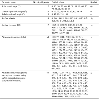
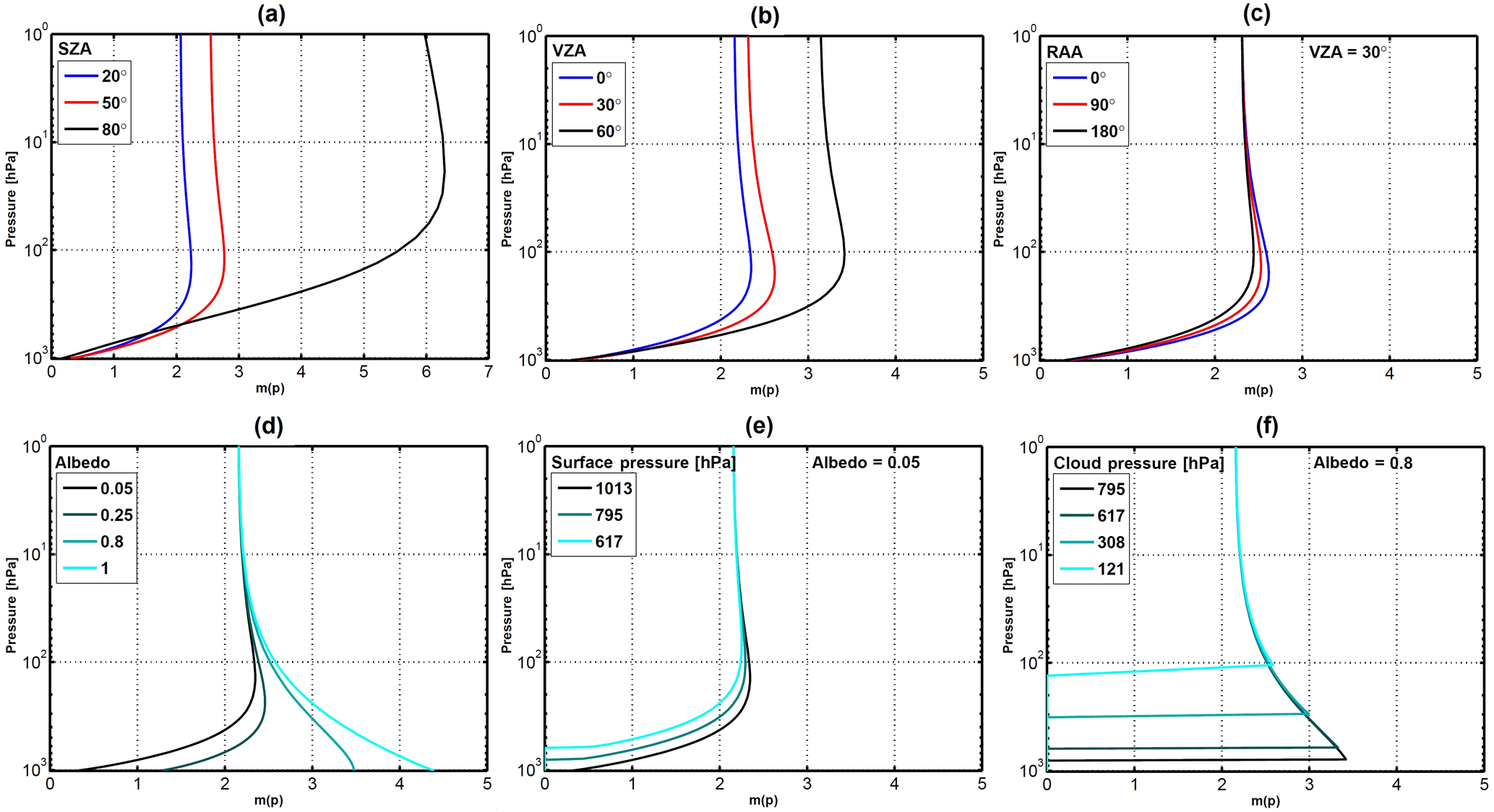
Figure 6Variation of the altitude-dependent air mass factor with (a) solar zenith angle, (b) viewing zenith angle, (c) relative azimuth angle between the sun and the satellite, (d) surface albedo, (e) surface pressure for a weakly reflecting surface, and (f) surface pressure for a highly reflecting surface. Unless specified, the parameters chosen for the radiative transfer simulations are a solar zenith angle (SZA) of 30∘, a viewing azimuth angle (VZA) of 0∘, a relative azimuth angle (RAA) of 0∘, albedo of 0.05, surface pressure of 1063 hPa, and λ = 340 nm.
Figure 6 illustrates the dependency of m with the observation angles, i.e. θ0 (a), θ (b), and φ (c), and with scene conditions like As (d) and ps for a weakly (e) or highly reflecting surface (f) (symbols in Table 4). The decrease of sensitivity in the boundary layer is more important for large solar zenith angles and wide instrumental viewing zenith angles. The relative azimuth angle does have relatively less impact on the measurement sensitivity (note, however, that aerosols and BRDF effects are not included in those simulations). In the UV, surfaces not covered with snow have an albedo lower than 0.1, while snow and clouds generally present larger albedos. For a weakly reflecting surface, the sensitivity decreases near the ground because photons are mainly scattered, and scattering can take place at varying altitudes. Larger values of the surface albedo increase the fraction of reflected compared to scattered photons, increasing measurement sensitivity to tropospheric absorbers near the surface. Over snow or ice also multiple scattering can play an important role further increasing the sensitivity close to the surface.
Altitude-dependent AMFs are calculated with the VLIDORT v2.6 radiative transfer model (Spurr, 2008a), at 340 nm, using an US standard atmosphere, for a number of representative viewing geometries, surface albedos, and surface pressures (used both for ground and cloud surface pressures), and stored in a LUT. Altitude-dependent AMFs are then interpolated within the LUT for each particular observation condition and interpolated vertically on the pressure grid of the a priori profile, defined within the TM5-MP model (Williams et al., 2017). Linear interpolations are performed in cos(θ0), cos(θ), relative azimuth angle, and surface albedo, while a nearest neighbour interpolation is performed in surface pressure. The parameter values chosen for the LUT are detailed in Table 4. In particular, the grid of surface pressure is very thin near the ground in order to minimize interpolation errors caused by the generally low albedo of ground surfaces. Indeed, as illustrated by Fig. 6e and f, the variation of the altitude-dependent AMFs is more discontinuous with surface elevation (low reflectivity) than with cloud altitude (high reflectivity). Furthermore, the LUT and model pressures are scaled to their respective surface pressures in order to avoid extrapolations outside the LUT range.
Treatment of partly cloudy scenes
The AMF calculations for TROPOMI will use the cloud fraction (fc), cloud albedo (Acloud), and cloud pressure (pcloud) from the S5P operational cloud retrieval, treating clouds as Lambertian reflectors (OCRA/ROCINN-CRB; Loyola et al., 2018). The applied cloud correction is based on the independent pixel approximation (Martin et al., 2002; Boersma et al., 2004), in which an inhomogeneous satellite pixel is considered as a linear combination of two independent homogeneous scenes, one completely clear and the other completely cloudy. The intensity measured by the instrument for the entire scene is decomposed into the contributions from the clear-sky and cloudy fractions. Accordingly, for each vertical layer, the altitude-dependent AMF of a partly cloudy scene is a combination of two AMFs, calculated, respectively, for the cloud-free and cloudy fractions of the scene:
where ml_clear is the altitude-dependent air mass factor for a completely cloud-free pixel, ml_cloud is the altitude-dependent air mass factor for a completely cloudy scene, and the cloud radiance fraction wc is defined as
Iclear and Icloud are, respectively, the radiance intensities for clear-sky and cloudy scenes whose values are calculated with VLIDORT at 340 nm and stored in LUTs with the same grids as the altitude-dependent air mass factors. ml_clear and Iclear are evaluated for a surface albedo As and a surface pressure ps, while ml_cloud and Icloud are estimated for a cloud albedo Acloud and at the cloud pressure pcloud. Note that the variations of the cloud albedo are directly related to the cloud optical thickness. Strictly speaking, in a Lambertian (reflective) cloud model approach, only thick clouds can be represented (one should keep in mind that still the penetration of photons into the cloud is not covered by the Lambertian model). An effective cloud fraction corresponding to an effective cloud albedo of 0.8 () can be defined in order to transform optically thin clouds into equivalent optically thick clouds of reduced horizontal extent. In such altitude-dependent air mass factor calculations, a single cloud top pressure is assumed within a given viewing scene. For low effective cloud fractions (feff lower than 10 %), the cloud top pressure retrieval is generally highly unstable and it is therefore reasonable to consider the observation as a clear-sky pixel (i.e. the cloud fraction is set to 0) in order to avoid unnecessary error propagation through the retrievals. This 10 % threshold might be adjusted according to the quality of the cloud product (Veefkind et al., 2016; Loyola et al., 2018).
It should be noted that this formulation of the altitude-dependent AMF for a partly cloudy pixel implicitly includes a correction for the HCHO column lying below the cloud and therefore not seen by the satellite, the so-called “ghost column”. Indeed, the total AMF calculation as expressed by Eqs. (7) and (8) assumes the same a priori vertical profile in both cloudy and clear parts of the pixel and implies an integration of the profile from the top of atmosphere to the ground, for each fraction of the scene. The ghost column information is thus coming from the a priori profiles. For this reason, observations with cloud fractions feff larger than 30 % are assigned with a poor quality flag and have to be used with caution.
Aerosols
The presence of aerosol in the observed scene may affect the quality of the retrieval. No explicit treatment of aerosols (absorbing or not) is foreseen in the operational algorithm as there is no general and easy way to treat the aerosols effect on the retrieval. At computing time, the aerosol parameters (extinction profile, single scattering albedo, etc.) are unknown. However, the information on the AAI (Stein Zweers et al., 2016) will be included in the L2 HCHO files as it gives information to the user on the presence of absorbing aerosols and the affected data should be used and interpreted with care.
A priori vertical profile shapes
Formaldehyde concentrations decrease with altitude as a result of the near-surface sources of short-lived NMVOC precursors, the temperature dependence of CH4 oxidation, and the altitude dependence of photolysis. The profile shape varies according to local NMHC sources, boundary layer depth, photochemical activity, and other factors.
To resolve this variability in the TROPOMI near-real-time (NRT) HCHO product, daily forecasts calculated with the TM5-MP chemical transport model (Huijnen et al., 2010; Williams et al., 2017) will be used to specify the vertical profile shape of the HCHO distribution. TM5-MP will also provide a priori profile shapes for the NO2, SO2, and CO retrievals. For the QA4ECV OMI products, high-resolution TM5-MP model runs were performed for the period 2004–2016, and the model profiles from this run are used for both HCHO and NO2 retrievals.
TM5-MP is operated with a spatial resolution of 1∘ × 1∘ in latitude and longitude and with 34 sigma pressure levels up to 0.1 hPa in the vertical direction. TM5-MP uses 3-hourly meteorological fields from the European Centre for Medium Range Weather Forecast (ECMWF) operational model (ERA-Interim reanalysis data for reprocessing, and the operational archive for real-time applications and forecasts). These fields include global distributions of wind, temperature, surface pressure, humidity, (liquid and ice) water content, and precipitation.
Table 5Prior information datasets used in the air mass factor calculation in the S5P HCHO operational algorithm and in the QA4ECV OMI algorithm.
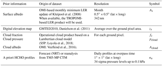
For the calculation of the HCHO air mass factors, the profiles are linearly interpolated in space and time, at pixel centre and local overpass time, through a model time step of 30 min. To reduce the errors associated to topography and the lower spatial resolution of the model compared to the TROPOMI 3.5 × 7 km2 spatial resolution, the a priori profiles need to be rescaled to effective surface elevation of the satellite pixel. Following Zhou et al. (2009) and Boersma et al (2011), the TM5-MP surface pressure is converted by applying the hypsometric equation and the assumption that the temperature changes linearly with height:
where ps,TM5 and TTM5 are the TM5-MP surface pressure and temperature, Γ=0.0065 K m−1 the lapse rate, zTM5 the TM5-MP terrain height, and zs surface elevation for the satellite ground pixel from a digital elevation map at high resolution. R = 287 J kg−1 K−1 is the gas constant for dry air, and g = 9.8 ms−2 is the gravitational acceleration.
The pressure levels for the a priori HCHO profiles are based on the improved surface pressure level ps: , al and bl being the constants that effectively define the vertical coordinate (Table 13).

Figure 7Yearly averaged map of tropospheric air mass factors at 340 nm using the QA4ECV OMI HCHO algorithm. A priori HCHO profiles from high-resolution TM5-MP model runs have been used. The IPA cloud correction is applied for effective cloud fractions feff larger than 10 %. Observations with feff larger than 30 % have been filtered out.
Yearly averaged OMI air mass factors obtained using prior information summarized in Table 5, in particular TM5-MP HCHO profiles, are presented in Fig. 7 in order to give an overview of the tropospheric AMF values and their global regional variations.
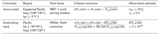
2.2.3 Across-track and zonal reference sector correction
Residual latitude-dependent biases in the columns, due to unresolved spectral interferences, are known to remain a limiting factor for the retrieval of weak absorbers such as HCHO. Retrieved HCHO slant columns can present large offsets depending on minor changes in the fit settings and minor instrumental spectral inaccuracies. Resulting offsets are generally global but also show particular dependencies, mainly with detector row (across track) and with latitude (along track). In the case of a 2-D-detector array such as OMI or TROPOMI, across-track striping can possibly arise due to imperfect calibration and different dead/hot pixel masks for the CCD detector regions. Offset corrections are also meant to handle some effects of the time-dependent degradation of the instrument.
A large part of the resulting systematic HCHO slant column uncertainty is reduced by the application of a background correction, which is based on the assumption that the background HCHO column observed over remote oceanic regions (Pacific Ocean) is only due to methane oxidation. The natural background level of HCHO is well estimated from chemistry model simulations of CH4 oxidation (). It ranges from 2 to 4 × 10¹⁵ molec cm−2, depending on the latitude and the season (De Smedt et al., 2008, 2015; González Abad et al., 2015).
For the HCHO retrieval algorithm, we use a two-step normalization of the slant columns (see Fig. 8 and Table 6).
-
textitAcross track. The mean HCHO slant column is determined for each row in the reference sector around the Equator ([−5∘, 5∘], [180∘, 240∘]). Data selection is based on the slant column errors from the DOAS fit and on the cloud fraction (threshold values are given in Table 6). Those mean HCHO values are subtracted from all the slant columns of the same day, as a function of the row. The aim is to reduce possible row-dependent offsets. In the case were solar irradiance are used as reference, those offsets can exceed 2 × 10¹⁶ molec cm−2 (see the first panel of Fig. 8). They are reduced below 1015 molec cm−2 by this first step or when row averaged radiances are used as reference, as in the QA4ECV algorithm (middle panel of Fig. 8).
-
Along track. The latitudinal dependency of the across-track corrected HCHO SCs is modelled by a polynomial fit through their mean values, all rows combined, in 5∘ latitude bins in the reference sector ([−90∘, 90∘], [180∘, 240∘]). Again, data selection is based on the slant column errors from the DOAS fit and on the cloud fraction.
These two corrections are applied to the global slant columns so that in the reference sector, the mean background corrected slant columns () are centred around zero (lower panel of Fig. 8).
To the corrected slant columns, the background HCHO values from a model have to be added. A latitude-dependent polynomial is fitted daily through 5∘ latitude bin means of those modelled values in the reference sector. Corresponding values are added to all the columns of the day. Strictly speaking, those background values should be slant columns, derived as the product of AMFs in the reference sector (M0) with HCHO vertical columns from the model () (González Abad et al., 2015). However, this option requires the storage of the slant columns, the AMFs, and their errors in a separate database (QA4ECV algorithm and S5P option; see Eq. 11). An approximate solution is to add as background the constant vertical column from the model (), thus neglecting the variability of the M0∕M ratio. This is the current implementation in the S5P algorithm, which will be updated with Eq. (11) after launch. For NRT purposes, the evaluation in the reference sector is made using a moving time window of 1 week. For offline processing, the reference sector correction can be refined by using daily evaluations.
Figure 3 presents some examples of monthly and regionally averaged vertical columns, together with the contribution of Nv,0. It should be realized that this contribution accounts for 20 to 50 % of the vertical columns, as expected from the large contribution of methane oxidation to the total HCHO column (Stavrakou et al., 2015).
Table 7Summary of the different error sources considered in the HCHO slant column uncertainty budget.
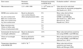
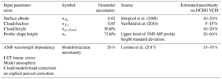
Table 8Summary of the different error sources considered in the air mass factor uncertainty budget.
3.1 Uncertainty formulation by uncertainty propagation
The total uncertainty on the HCHO vertical column is composed of many sources of (random and systematic) errors. In part those are related to the measuring instrument, such as errors due to noise or knowledge of the slit function. In a DOAS-type algorithm, those instrumental errors propagate into the uncertainty of the slant columns. Other types of error can be considered as model errors and are related to the representation of the observation physical properties that are not measured. Examples of model errors are errors on the trace gas absorption cross sections, the treatment of clouds and errors of the a priori profiles. Model errors can affect the slant columns, the AMFs, or the applied background corrections.
A formulation of the uncertainty can be derived analytically by uncertainty propagation, starting from the equation of the vertical column (Eq. 11), which directly results from the different retrieval steps. As the main algorithm steps are performed independently, they are assumed to be uncorrelated. The total uncertainty on the tropospheric vertical column can be expressed as (Boersma et al., 2004; De Smedt et al., 2008)
where σN,s, σM, , σM,0, and are, respectively, the uncertainties on the slant column, the air mass factor, the slant column correction, the air mass factor, and the model vertical column in the reference sector (indicated by suffix 0). For each of these categories, the following sections provide more details on the implementation of the uncertainty estimate in the HCHO algorithm. A discussion of the sources of uncertainties and, where possible, their estimated size are presented, as well as their spatial and temporal patterns.
Note that in the current implementation of the operational processor, M0=M, and the uncertainty formulation therefore reduces to
Complementing this uncertainty propagation analysis, total column averaging kernels (A) based on the formulation of Eskes and Boersma (2003) are estimated. Column averaging kernels provide essential information when comparing measured columns with e.g. model simulations or correlative validation datasets, because they allow removal of the effect of the a priori HCHO profile shape used in the retrieval (see Appendix C; Boersma et al., 2004, 2016).
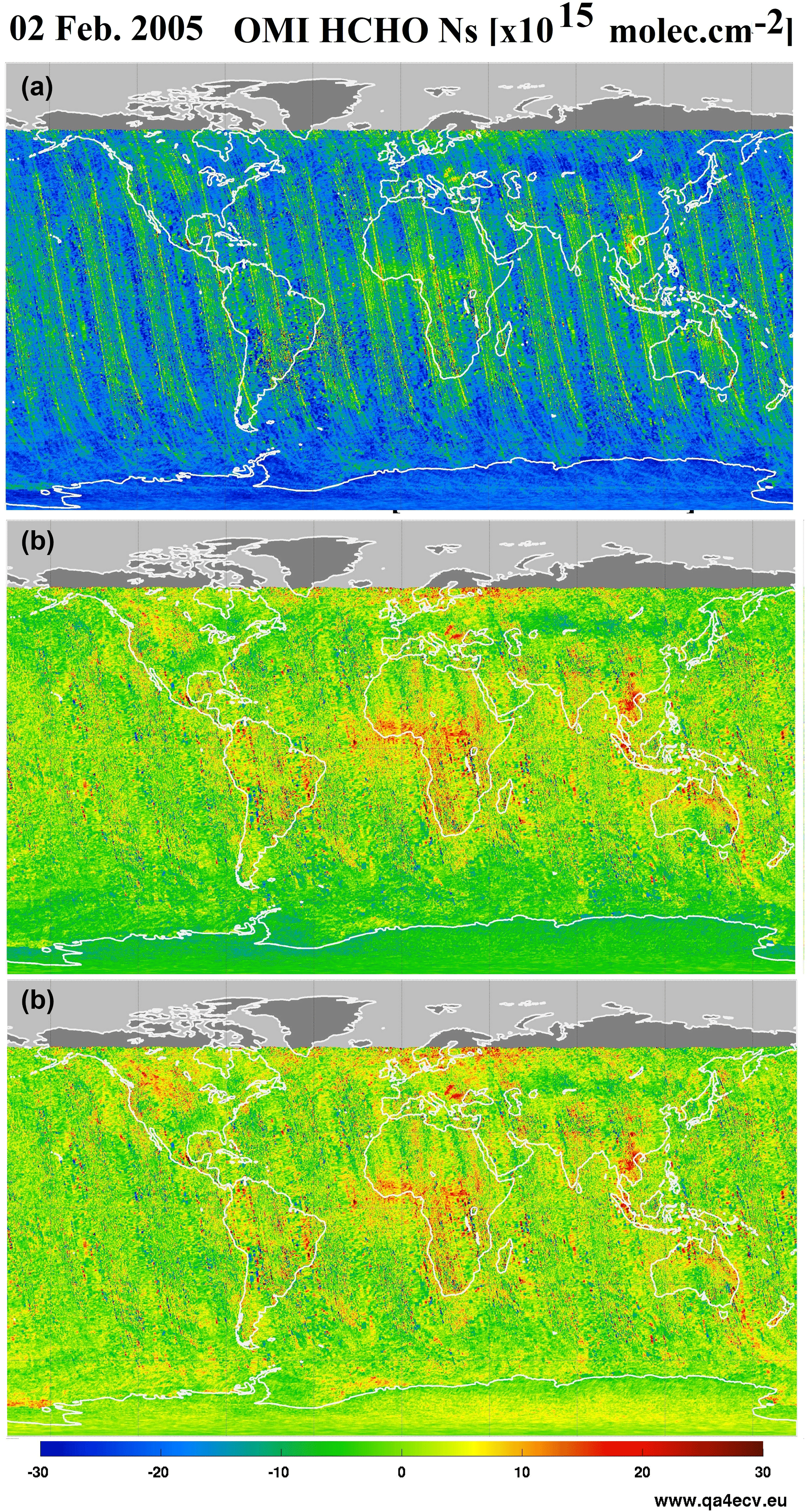
Figure 8Illustration of the across-track and zonal reference sector correction steps applied to 1 day of OMI HCHO slant columns (2 February 2005). Panel (a) shows the uncorrected slant columns obtained using as DOAS reference spectrum the solar irradiance. Panel (b) shows the same slant columns after the first across-track correction step or when row averaged radiances selected in the Pacific Ocean are used as reference. Panel (c) shows the final background corrected slant columns ΔNs.
Section 3.2 presents our current estimates of the precision (random uncertainty) and the trueness (systematic uncertainty) that can be expected for the TROPOMI HCHO vertical columns. They are discussed along with the product requirements (Sect. 2.1).
3.1.1 Errors on the slant columns
Error sources that contribute to the total uncertainty on the slant column originate both from instrument characteristics and from errors in the DOAS slant column fitting procedure itself.
The retrieval noise for individual observations is limited by the SNR of the spectrometer measurements. A good estimate of the random variance of the reflectance (which results from the combined noise of radiance and reference spectra) is given by the reduced χ2 of the fit, which is defined as the sum of squares (Eq. 4) divided by the number of degrees of freedom in the fit. The covariance matrix (Σ) of the linear least-squares parameter estimate is then given by
where k is the number of spectral pixels in the fitting interval, n is the number of parameters to fit, and the matrix A(jxk) is formed by the cross sections. For each absorber j, the value is usually called the slant column error (SCE or ).
Equation (16) does not take into account systematic errors, which are mainly dominated by slit function and wavelength calibration uncertainties, absorption cross-section uncertainties, interferences with other species (O3, BrO, or O4), or uncorrected stray light effects. The choice of the retrieval interval can have a significant impact on the retrieved HCHO slant columns. The systematic contributions to the slant column errors are empirically estimated from sensitivity tests (see Table 7) and can be viewed as part of the structural uncertainty (Lorente et al., 2017). However, remaining systematic offsets and zonal biases are greatly reduced by the reference sector correction. All effects summed in quadrature, the various contributions are estimated to account for an additional systematic uncertainty of 20 % of the background-corrected slant column:
The total uncertainty on slant columns is then

Figure 9First panel: TM5-MP HCHO profiles extracted in June over the equatorial Pacific ocean (blue) and over Beijing (red). Those profiles have been used to calculated the tropospheric air mass factors shown in the panels (a–e), representing the AMF dependence on (a) the surface albedo, (b) the cloud altitude, and (c–e) the cloud fraction. In all cases, we consider a nadir view and a solar zenith angle of 30∘. In panel (a) the pixel is cloud-free, in panel (b) the albedo is 0.02 and the effective cloud fraction is 0.5, and in panels (c–e) the ground albedo is 0.02 and the cloud pressure is, respectively, 966, 795, and 540 hPa.
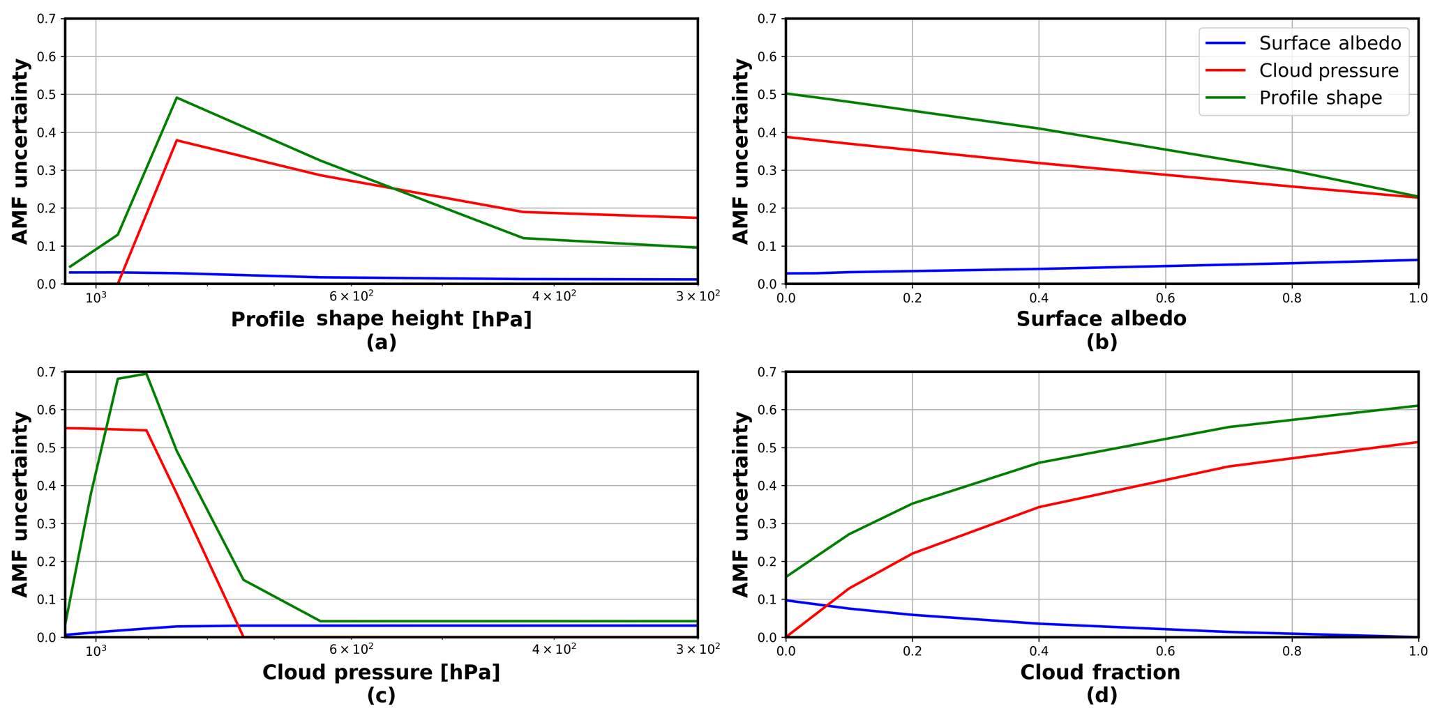
Figure 10AMF uncertainty related to profile shape, cloud pressure, and surface albedo errors, as a function of different observation conditions. In all cases, we consider a nadir-viewing and a solar zenith angle of 30∘. By default, fixed values have been used. The surface pressure is 1063 hPa, the albedo is 0.05, the effective cloud fraction is 0.5, and the profile height and cloud pressure are 795 hPa.
3.1.2 Errors on air mass factors
The uncertainties on the AMF depend on input parameter uncertainties and on the sensitivity of the AMF to each of them. This contribution is broken down into the squared sum (Boersma et al., 2004, De Smedt et al., 2008):
The contribution of each parameter to the total air mass factor error depends on the observation conditions. The air mass factor sensitivities (), i.e. the air mass factor derivatives with respect to the different input parameters, can be derived for any particular condition of observation using the altitude-dependent AMF LUT and using the model profile shapes (see Fig. 9). In practice, a LUT of AMF sensitivities has been created using coarser grids than the AMF LUT and one parameter describing the shape of the profile: the profile height, i.e. the altitude (pressure) below which resides 75 % of the integrated HCHO profile. is approached by , where sh is half of the profile height. Relatively small variations of this parameter have a strong impact on the total air mass factors, because altitude-resolved air mass factors decrease quickly in the lower troposphere, where the HCHO profiles peak (Fig. 6).
The uncertainties σA,s, , and σs,h are typical uncertainties on the surface albedo, cloud fraction, cloud top pressure, and profile shape, respectively. They are estimated from the literature or derived from comparisons with independent data (see Table 8). Together with the sensitivity coefficients, these give the first four contributions on the right of Eq. (19). The fifth term on the right of Eq. (19) represents the uncertainty contribution due to possible errors in the AMF model itself (Lorente et al., 2017). We estimate this contribution to 20 % of the AMF (see also Sect. 3.2.2).
Estimates of the AMF uncertainties and of their impact on the vertical column uncertainties are listed in Table 8 and represented in Fig. 10. They are based on the application of Eq. (19) to HCHO columns retrieved from OMI measurements. In Eq. (19), the impact of possible correlations between errors on parameters is not considered, such as the surface albedo and the cloud top pressure. Note also that errors on the solar angles, the viewing angles, and the surface pressure are supposed to be negligible, which is not totally true in practice, since Eq. (10) does not yield the true surface pressure but only a good approximation.
3.1.3 Surface albedo
A reasonable uncertainty on the albedo is 0.02 (Kleipool et al., 2008). This translates to an uncertainty on the AMF using the slope of the AMF as a function of the albedo and can be evaluated for each satellite pixel (Eq. 19). As an illustration, Fig. 9a shows the AMF dependence on the ground albedo for two typical HCHO profile shapes (remote profile in blue, emission profile in red). At 340 nm, the AMF sensitivity (the slope), is almost constant with albedo, being only slightly higher for low albedo values. As expected, the AMF sensitivity to albedo is higher for an emission profile peaking near the surface than for a background profile more spread in altitude. More substantial errors can be introduced if the real albedo differs considerably from what is expected, for example in the case of the sudden snowfall or ice cover. A snow and ice cover map will therefore be used for flagging such cases.
3.1.4 Clouds and aerosols
An uncertainty on the cloud fraction of 0.05 is considered, while an uncertainty on the cloud top pressure of 50 hPa is taken. Figure 9b shows the AMF variation with cloud altitude. The AMF is very sensitive to the cloud top pressure (the slope is steepest) when the cloud is located below or at the level of the formaldehyde peak. For higher clouds, the sensitivity of the AMF to any change in cloud pressure is very weak. As illustrated in Fig. 9c–e, for which a cloud top pressure of 966, 795, and 540 hPa is, respectively, considered, the sensitivity to the cloud fraction is mostly significant when the cloud lies below the HCHO layer.
The effect of aerosols on the AMFs are not explicitly considered in the HCHO retrieval algorithm. To a large extent, however, the effect of the non-absorbing part of the aerosol extinction is implicitly included in the cloud correction (Boersma et al., 2011). Indeed, in the presence of aerosols, the cloud detection algorithm is expected to overestimate the cloud fraction. Since non-absorbing aerosols and clouds have similar effects on the radiation in the UV–visible range, the omission of aerosols is partly compensated by the overestimation of the cloud fraction, and the resulting error on AMF is small, typically below 15 % (Millet et al., 2006; Boersma et al., 2011; Lin et al., 2014; Castellanos et al., 2015; Chimot et al., 2016). In some cases, however, the effect of clouds and aerosols will be different. For example, when the cloud height is significantly above the aerosol layer, clouds will have a shielding effect while the aerosol amplifies the signal through multiple scattering. This will result in an underestimation of the AMF. Absorbing aerosols have also a different effect on the AMFs, since they tend to decrease the sensitivity to HCHO concentration. In this case, the resulting error on the AMF can be as high as 30 % (Palmer et al., 2001; Martin et al., 2002). This may, for example, affect significantly the derivation of HCHO columns in regions dominated by biomass burning and over heavily industrialized regions. Shielding and reflecting effect can thus occur, depending on the observation, decreasing or increasing the sensitivity to trace gas absorption. It has been shown that uncertainties related to aerosols are reduced by spatiotemporal averaging (Barkley et al., 2012; Lin et al., 2014; Castellanos et al., 2015; Chimot et al., 2016). Furthermore, the applied cloud filtering effectively removes observations with the largest aerosol optical depth. In the HCHO product, observations with an elevated absorbing aerosol index will be flagged, to be used with caution.
3.1.5 Profile shape
This contribution to the total AMF error is the largest when considering monthly averaged observations. This is supported by validation results using Multi-Axis DOAS (MAX-DOAS) profiles measured around Beijing and Wuxi (see De Smedt et al., 2015; Wang et al., 2016). Taking into account the averaging kernels allows removal of the error related to the a priori profiles from the comparison, when validating the results against other modelled or measured profiles (see Appendix C).
3.1.6 Errors on the reference sector correction
This uncertainty includes contributions from the model background vertical column (see the recent study of Anderson et al., 2017), from the error on the air mass factor in the reference sector, and from the amplitude of the normalization applied to the HCHO columns. As mentioned in Sect. 3.1.1, we consider that is taken into account in Eq. (17). The uncertainty on the air mass factor in the reference sector σM,0 is calculated as in Eq. (19) and saved during the background correction step. Uncertainty on the model background has been estimated as the absolute values of the monthly averaged differences between two different CTM simulations in the reference sector: IMAGES (Stavrakou et al., 2009a) and TM5-MP (Huijnen et al., 2010). The differences range between 0.5 and 1.5 × 10¹⁵ molec cm−2.
3.2 HCHO error estimates and product requirements
This section presents estimates of the precision (random error) and trueness (systematic error) that can be expected for the TROPOMI HCHO vertical columns. These estimates are given in different NMVOC emission regions. Precision and trueness of the HCHO product are discussed against the user requirements.

Figure 11Estimated precision on the TROPOMI HCHO columns, in several NMVOC emission regions and at different spatial and temporal scales (from individual pixels to monthly averages in 20 × 20 km2 grids). These estimated are based on OMI observations in 2005, using observations with an effective cloud fraction lower than 40 %.
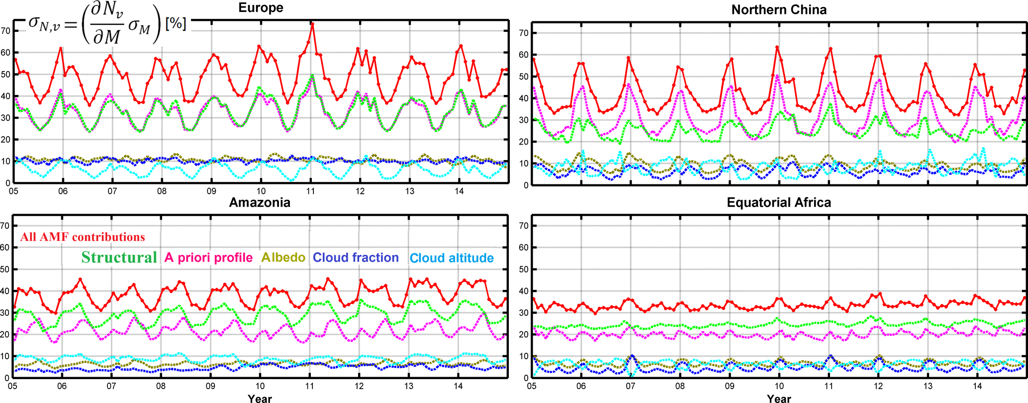
Figure 12Regional and monthly average of the relative systematic vertical column AMF-related uncertainties in several NMVOC emission regions, for the period 2005–2014. The five contributions to the systematic air mass factor uncertainty are shown: structural (green), a priori profile (pink), albedo (olive), cloud fraction (blue), and cloud altitude (cyan).
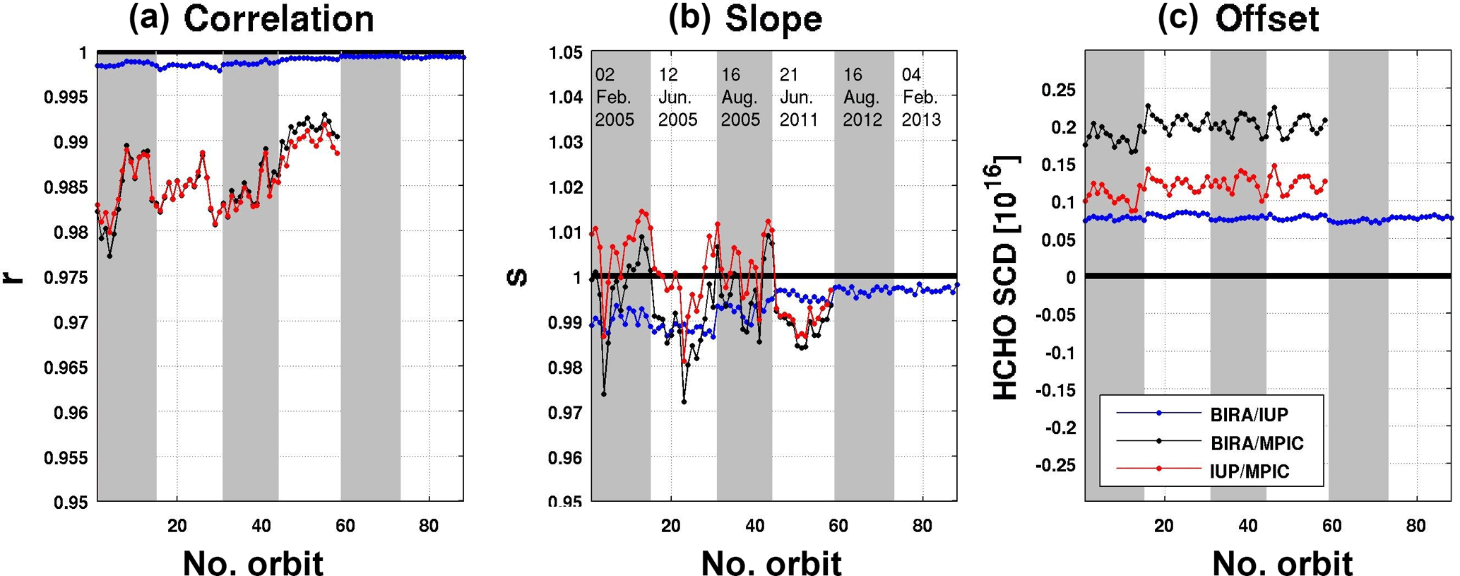
Figure 13Correlation (a), slope (b), and offset (c) from a linear regression performed for the common fit settings (see Table 11) for each orbit of OMI test days. A correlation plot for an example orbit is provided in the left panel of Fig. 14.
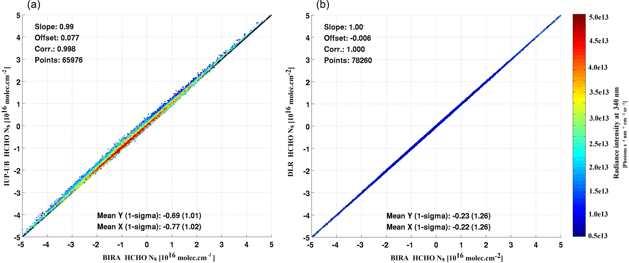
Figure 14Correlation plots of HCHO slant columns retrieved with the BIRA prototype algorithm and (a) the IUP-UB verification algorithm and (b) the operational processor, for OMI orbit number 2339 on 2 February 2005, including all pixels with SZA < 80∘.
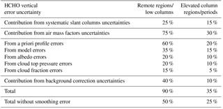
Table 10Estimated HCHO vertical column uncertainty budget for monthly averaged low and elevated columns (higher than 1 × 10¹⁶ molec cm−2). Contributions from the three retrieval steps are provided, as well as input parameter contributions.
3.2.1 Precision
When considering individual pixels, the total uncertainty is dominated by the random error on the slant columns. Our simulations and tests on real satellite measurements show that the precision by which the HCHO can be measured is well defined by the instrument signal-to-noise level. For the nominal SNR level (1000), the expected precision of single-pixel measurements is equivalent to the precision obtained with OMI HCHO retrievals (De Smedt et al., 2015), but with a ground pixel size of about 3.5 × 7 km2, i.e. 1 order of magnitude smaller in surface. Absolute values typically range between 7 and 12 × 1015 molec cm−2 for individual pixels, showing an increase as a function of the surface altitude and of the solar zenith angle. Relative values range between 100 and 300 %, depending on the observation scene. In the case of HCHO retrievals, for individual satellite ground pixels, the random error on the slant columns is the most important source of uncertainty on the total vertical column. It can be reduced by averaging the observations, but of course at the expense of a loss in time and/or spatial resolution.
The precision of the vertical columns provided in the L2 files corresponds to the precision of the slant column divided by the AMF (see Table 13). It is dependent on the AMFs and, therefore, on the observation conditions and on the cloud statistics. Figure 11 shows the vertical column precision that is expected for TROPOMI, based on OMI observations in 2005. Results are shown in several regions and at different spatial and temporal scales (from individual pixels to monthly averaged column in 20 × 20 km2 grids). The product requirements for HCHO measurements state a precision of 1.3 × 10¹⁵ molec cm−2. This particular requirement cannot be achieved with individual observations at full spatial resolution. However, as represented in Fig. 11, the requirement can be approached using daily observations at the spatial resolution of 20 × 20 km2 (close to the OMI resolution) or using monthly averaged columns at the TROPOMI resolution. The precision can be brought below 1 × 10¹⁵ molec cm−2 if a spatial resolution of 20 × 20 km2 is considered for monthly averaged columns.
3.2.2 Trueness
In this section, we present monthly averaged values of the systematic vertical columns uncertainties estimated for OMI retrievals between 2005 and 2014. The contribution of the AMF uncertainties is the largest contribution to the vertical column systematic uncertainties (see also Table 10). Figure 12 presents the VCD uncertainties due to AMF errors and the five considered contributions, over equatorial Africa and northern China, as example of tropical and mid-latitude sites. The largest contributions are from the a priori profile uncertainty and from the structural uncertainty (taken as 20 % of the AMF). In the case where the satellite averaging kernels are used for comparisons with external HCHO columns, the a priori profile contribution can be removed from the comparison uncertainty budget, leading to a total uncertainty in the range of 25 to 50 %. Table 10 wraps up the estimated relative contributions to the HCHO vertical column uncertainty in the case of monthly averaged columns for typical low and high columns.
Considering these estimates of the HCHO column trueness, the requirements for HCHO product (30 %) are achievable in regions of high emissions and for certain times of the year. In any case, observations need to be averaged to reduce random uncertainties at a level comparable or smaller than systematic uncertainties.
In the framework of the TROPOMI L2 WG and QA4ECV projects, extensive comparisons of the prototype (this paper), the verification (IUP-UB), and alternative scientific algorithms (MPIC, KNMI, WUR) have been conducted. All follow a common DOAS approach. Prototype and verification algorithms have been applied to both synthetic and OMI spectra. Here, we present a selection of OMI results. For a complete description of the verification algorithm as well as results and discussion of the retrievals applied to synthetic spectra, please refer to the TROPOMI verification report (Richter et al., 2015).
4.1 Harmonized DOAS fit settings using OMI test data
For this exercise, a common set of DOAS fit parameters has been agreed upon. The goal of the intercomparison of harmonized fit settings was to ensure that the software implementation of the different algorithms behaves as expected in a large range of realistic measurement scenarios. Another objective was to gain knowledge of the level of agreement or disagreement of results from different groups when using the same settings as well as of the main drivers for differences. Common and simple fit parameters based on the operational and verification algorithm were selected. They are summarized in Table 11.
The intercomparison of results using common settings allowed us to identify and fix several issues in the different codes, leading to an overall consolidation of the algorithms. It has been found that minor changes in the fit settings may lead to large offsets (±10 × 1015 molec cm−2) in the HCHO SCDs. However, an excellent level of agreement (±2 × 10¹⁵ molec cm−2) between the different retrieval codes was obtained after several iterations of the common settings. The main sources of discrepancies were found to be related to (1) the solar I0 correction applied on the O3 cross sections, (2) the intensity offset correction, (3) the details of the wavelength calibration of the radiance and irradiance spectra, and (4) the OMI slit functions and their implementation in the convolution tools (Boersma et al., 2015).
An overview of the final SCD comparison is shown on Fig. 13 for 6 test days at the beginning and the end of the OMI time series and for a particular OMI orbit on the left panel of Fig. 14. The correlation coefficient, slope, and offset of linear regression fits performed on each comparison orbit are displayed. The correlation of slant columns from BIRA and IUP-UB is extremely high in most cases. It is > 0.998 for all orbits. The slope of the regression line between BIRA and IUP-UB results is close to 1.0. There is a constant offset of less than 1 × 10¹⁵ molec cm−2. The comparison between MPIC results and the two other algorithms gives somehow lower correlations, but still larger than 0.98 from the beginning to the end of the OMI lifetime. Final deviations on OMI HCHO SCD when using common settings were found to be of maximum ±2 % (slope) and 2.5 × 10¹⁵ molec cm−2. When relating the remaining differences in retrieved SCDs using common settings to the slant column errors from the DOAS fit (), it can be concluded that the differences between the results are significantly smaller than the uncertainties (from 10 to 20 % of ). Moreover, remaining offsets in SCDs are further reduced by the background correction procedure.
4.2 Verification of the operational implementation
A similar intercomparison exercise was performed with the operational algorithm UPAS, developed at DLR, but using the exact settings of the prototype algorithm as detailed in Table 2. An example of resulting correlation fit is shown in the right panel of Fig. 14 for the same OMI orbit as for the comparison with the IUP-UB results. The level of agreement between the prototype and operational results is found to be almost perfect (correlation coefficient of 1, slope of 1.003 and offset of less than 0.2 × 10¹⁵ molec cm−2) and thus very satisfactory considering the sensitivity on small implementation changes.
Table 12Data and measurement types used for the validation of satellite HCHO columns. The information content of each type of measurement is qualitatively represented by the number of crosses.
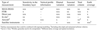
1Surface measurements that could be combined with regional
modelling. 2Including ultra-light and unmanned airborne
vehicles.
3Up to 2–3 km. 4Profiles generally need to be
extrapolated. 5Different daily coverage and spatial resolutions.
Independent validation activities are proposed and planned by the S5P Validation Team (Fehr, 2016) and within the ESA S5P Mission Performance Center (MPC). The backbone of the formaldehyde validation is the MAX-DOAS and FTIR networks operated as part of the Network for the Detection of Atmospheric Composition Change (NDACC, http://www.ndsc.ncep.noaa.gov/) complemented by Pandonia (http://pandonia.net/) and national activities. In addition, model datasets will be used for validation as well as independent satellite retrievals. Finally, airborne campaigns are planned to support the formaldehyde and other trace gases validation.
5.1 Requirements for validation
To validate the TROPOMI formaldehyde data products, comparisons with independent sources of HCHO measurements are required. This includes comparisons with ground-based measurements, aircraft observations, and satellite datasets from independent sensors and algorithms. Moreover, not only information on the total (tropospheric) HCHO column is needed but also information on its vertical distribution, especially in the lowest 3 km where the bulk of formaldehyde generally resides. In this altitude range, the a priori vertical profile shapes have the largest systematic impact on the satellite column errors. HCHO and aerosol profile measurements are therefore needed.
The diversity of the NMVOC species, lifetimes, and sources (biogenic, biomass burning, or anthropogenic) calls for validation data in a large range of locations worldwide (tropical, temperate and boreal forests, urban and suburban areas). Continuous measurements are needed to obtain good statistics (both for ground-based measurements and for satellite columns) and to capture the seasonal variations. Validation and assessment of consistency with historical satellite datasets require additional information on the HCHO diurnal variation, which depends on the precursor emissions and the local chemical regime.
The main emphasis is on quality assessment of retrieved HCHO column amounts on a global scale and over long time periods. The validation exercise will establish whether HCHO data quality meets the requirements of geophysical research applications like long-term trend monitoring on the global scale, NMVOC source inversion, and research on the budget of tropospheric ozone. In addition, the validation will investigate the consistency between TROPOMI HCHO data and HCHO data records from other satellites.
5.2 Reference measurement techniques
Table 12 summarizes the type of data and measurements that can be used for the validation of the TROPOMI HCHO columns. The advantages and limitations of each technique are discussed. It should be noted that, unlike tropospheric O3 or NO2, the stratospheric contribution to the total HCHO column can be largely neglected, which simplifies the interpretation of both satellite and ground-based measurements.
The MAX-DOAS measurement technique has been developed to retrieve stratospheric and tropospheric trace gas total columns and profiles. The most recent generation of MAX-DOAS instruments allows for measurement of aerosols and a number of tropospheric pollutants, such as NO2, HCHO, SO2, O4, and CHOCHO (e.g. Irie et al., 2011). With the development of operational networks such as Pandonia, it is anticipated that many more MAX-DOAS instruments will become available in the near future to extend validation activities in other areas where HCHO emissions are significant. The locations where HCHO measurements are required are reviewed in the next section. Previous comparisons between GOME-2 and OMI HCHO monthly averaged columns with MAX-DOAS measurements recorded by BIRA-IASB in the Beijing city centre and in the suburban site of Xianghe showed that the systematic differences between the satellite and ground-based HCHO columns (about 20 to 40 %) are almost completely explained when taking into account the vertical averaging kernels of the satellite observations (De Smedt et al., 2015; Wang et al., 2017), showing the importance of validating the a priori profiles as well.
HCHO columns can also be retrieved from the ground using FTIR spectrometers. In contrast to MAX-DOAS systems which essentially probe the first 2 km of the atmosphere, FTIR instruments display a strong sensitivity higher up in the free troposphere and are thus complementary to MAX-DOAS (Vigouroux et al., 2009). The deployment of FTIR instruments of relevance for HCHO is mostly taking place within the NDACC network. Within the project NIDFORVal (S5P Nitrogen Dioxide and Formaldehyde Validation using NDACC and complementary FTIR and UV–visible networks), the number of FTIR stations providing HCHO time series has been raised from only 4 (Vigouroux et al., 2009; Jones et al., 2009; Viatte et al., 2014; Franco et al., 2015) to 21. These stations are covering a wide range of HCHO concentrations, from clean Arctic or oceanic sites to suburban and urban polluted sites, as well as sites with large biogenic emissions such as Porto Velho (Brazil) or Wollongong (Australia).
Although ground-based remote-sensing DOAS and FTIR instruments are naturally best suited for the validation of column measurements from space, in situ instruments can also bring useful information. This type of instrument can only validate surface HCHO concentrations, and therefore additional information on the vertical profile (e.g. from regional modelling) is required to make the link with the satellite retrieved column. However, in situ instruments (where available) have the advantage to be continuously operated for pollution monitoring in populated areas, allowing for extended and long-term comparisons with satellite data (see e.g. Dufour et al., 2009). Although more expensive and with a limited time and space coverage, aircraft campaigns provide unique information on the HCHO vertical distributions (Zhu et al., 2016).

Figure 15HCHO columns over northern China as observed with GOME (in blue), SCIAMACHY (in black), GOME-2 (in green), and OMI (in red) (De Smedt et al., 2008, 2010, 2015).
5.3 Deployment of validation sites
Sites operating correlative measurements should preferably be deployed at locations where significant NMVOC sources exist. This includes the following:
-
Tropical forests (Amazonian forest, Africa, Indonesia). The largest HCHO columns worldwide are observed over these remote areas that are difficult to access. Biogenic and biomass burning emissions are mixed. A complete year is needed to discriminate the various effects on the HCHO retrieval. Clouds tend to have more systematic effects in tropical regions. Aircraft measurements are needed over biomass burning areas.
-
Temperate forests (south-eastern US, China, Eastern Europe). In summertime, HCHO columns are dominated by biogenic emissions. Those locations are useful to validate particular a priori assumptions such as model isoprene chemistry and OH oxidation scheme. Measurements are mostly needed from April to September.
-
Urban and suburban areas (Asian cities, California, European cities). Anthropogenic NMVOCs are more diverse and have a weaker contribution to the total HCHO column than biogenic NMVOCs. This type of signal is therefore more difficult to validate. Continuous observations at mid-latitudes over a full year are needed, to improve statistics.
For adequate validation, the long-term monitoring should be complemented by dedicated campaigns. Ideally such campaigns should be organized in appropriate locations such as south-eastern US and Alabama, where biogenic NMVOCs and biogenic aerosols are emitted in large quantities during summertime and should include both aircraft and ground-based components.
5.4 Satellite–satellite intercomparisons
Satellite–satellite intercomparisons of HCHO columns are generally more straightforward than validation using ground-based correlative measurements. Such comparisons are evaluated in a meaningful statistical sense focusing on global patterns and regional averages, seasonality, scatter of values and consistency between results and reported uncertainties. When intercomparing satellite measurements, special care has to be taken for
-
differences in spatial resolutions, resulting in possible offsets between satellite observations (van der A et al., 2008; De Smedt et al., 2010; Hilboll et al., 2013);
-
differences in overpass times, which hold valuable geophysical information about diurnal cycles in emissions and chemistry (De Smedt et al., 2015; Stavrakou et al., 2015);
-
differences in a priori assumptions;
-
differences in the cloud algorithms and cloud correction schemes.
Assessing the consistency between successive satellite sensors is essential to allow for scientific studies making use of the combination of several sensors. For example, trends in NMVOC emissions have been successfully derived from GOME(-2), SCIAMACHY, and OMI measurements (Fig. 15). It is anticipated that TROPOMI and the next GOME-2 instruments – OMPS, GEMS, TEMPO, and the future Sentinels 4 and 5 – will allow to extend these time series.
The retrieval algorithm for the TROPOMI formaldehyde product generation is based on the heritage from algorithms successfully developed for the GOME, SCIAMACHY, GOME-2, and OMI sensors. A double-interval fitting approach is implemented, following an algorithm baseline demonstrated on the GOME-2 and OMI sensors. The HCHO retrieval algorithm also includes a post-processing across-track reference sector correction to minimize OMI-type striping effects, if any. Additional features for future processor updates include the use of a larger fitting interval (if the quality of the recorded spectra allows it), daily earthshine radiance as reference selected in the remote Pacific, spectral outlier screening during the fitting procedure (spike removal algorithm), and a more accurate background correction scheme (as developed for the QA4ECV product).
A detailed uncertainty budget is provided for every satellite observation. The precision of the HCHO tropospheric column is expected to come close to the COPERNICUS product requirements in regions of high emissions and, at mid-latitude, for summer (high sun) conditions. The trueness of the vertical columns is also expected to be improved, owing to the use of daily forecasts for the estimation of HCHO vertical profile shapes that will be provided by a new version of the TM5-MP model, running at the spatial resolution of 1∘ × 1∘ degree in latitude and longitude.
The validation of satellite retrievals in the lower troposphere is known to be challenging. Ground-based measurements, where available, often sample the atmosphere at different spatial and temporal scales than the satellite measurements, which leads to ambiguous comparisons. Additional correlative measurements are needed over a variety of regions, in particular in the tropics and at the suburban level in mid-latitudes. These aspects are covered by a number of projects developed in the framework of the TROPOMI validation plan (Fehr, 2016).
This paper is a description of algorithm for TROPOMI/S5P. There is no existing dataset yet. The QA4ECV OMI HCHO product is available at https://doi.org/10.18758/71021031 (De Smedt et al., 2017).
| A | Averaging kernel |
| AMF | Air mass factor |
| AOD | Aerosol optical depth |
| AAI | Aerosol absorbing index |
| ATBD | Algorithm Theoretical Basis Document |
| BIRA-IASB | Royal Belgian Institute for Space Aeronomy |
| BrO | Bromine monoxide |
| BRDF | Bidirectional reflectance distribution function |
| CH4 | Methane |
| CO | Carbon monoxide |
| CAPACITY | Composition of the Atmosphere: Progress to Applications in the user CommunITY |
| CCD | Charged coupled device |
| CRB | Clouds as reflecting boundaries |
| CTM | Chemical transport model |
| DOAS | Differential optical absorption spectroscopy |
| DU | Dobson unit (1 DU = 2.6867 × 10¹⁶ molecules cm−2) |
| ECMWF | European Centre for Medium Range Weather Forecast |
| ESA | European Space Agency |
| FWHM | Full width half maximum |
| GMES | Global Monitoring for Environment and Security |
| GOME | Global Ozone Monitoring Experiment |
| HCHO | Formaldehyde (or H2CO) |
| IPA | Independent pixel approximation |
| IR | Infrared |
| ISRF L2 | Instrument Spectral Response Function Level 2 |
| L2WG | Level 2 Working Group |
| LER | Lambertian equivalent reflector |
| VLIDORT | Vector LInearized Discrete OrdinateRadiative Transfer |
| LOS | Line-of-sight angle |
| LS | Lower stratosphere |
| LUT | Look-up table |
| MAX-DOAS | Multi-Axis DOAS |
| MPC | Mission Performance Center |
| NDACC | Network for the Detection ofAtmospheric Composition Change |
| NMVOC | Non-methane volatile organic compound |
| NO2 | Nitrogen dioxide |
| NRT | Near-real time |
| OCRA | Optical Cloud Recognition Algorithm |
| OD | Optical depth |
| O3 | Ozone |
| OMI | Ozone Monitoring Instrument |
| OMPS | Ozone Mapping Profiler Suite |
| PCA | Principal component analysis |
| QA4ECV | Quality Assurance For Essential Climate Variables |
| RAA | Relative azimuth angle |
| ROCINN | Retrieval Of Cloud Information using Neural Networks |
| RTM | Radiative transfer model |
| S5P | Sentinel-5 Precursor |
| S5 | Sentinel-5 |
| SAA | Solar azimuth angle |
| SCIAMACHY | SCanning Imaging AbsorptionspectroMeter for Atmospheric ChartograpHY |
| SCD | Slant column density |
| SNR | Signal-to-noise ratio |
| SO2 | Sulfur dioxide |
| SOW | Statement of work |
| SZA | Solar zenith angle |
| TM 4/5 | Data assimilation/chemistry transport model (version 4 or 5) |
| TROPOMI | Tropospheric Monitoring Instrument |
| UPAS | Universal Processor for UV/VIS Atmospheric Spectrometers |
| UV | Ultraviolet |
| VCD | Vertical column density |
In addition to the main product results, such as HCHO slant column, tropospheric vertical column, and air mass factor, the L2 data files contain a number of additional ancillary parameters and diagnostic information.
Table B1Selective list of output fields in the TROPOMI HCHO product. Scanline and ground_pixel are, respectively, the number of pixels in an orbit along track and across track. Layer is the number of vertical levels in the averaging kernels and the a priori profiles.
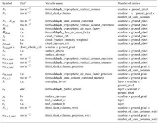
* Multiplication factor to convert mol m−2 to molec cm−2: 6.022 × 10¹⁹.
Retrieved satellite quantities always represent a weighted average over all parts of the atmosphere that contribute to the signal observed by the satellite instrument. The DOAS total column retrieval is implicitly dependant on the a priori trace gas profile na. Radiative transfer calculations account for the sensitivity of the measurement to the HCHO concentrations at all altitudes and these sensitivities are weighted with the assumed a priori profile shape to produce the vertical column. The averaging kernel (A) is proportional to the measurement sensitivity profile and provides the relation between the retrieved column Nv and the true tracer profile x (Rodgers, 2000; Rodgers and Connor, 2003):
where the profiles are expressed in partial columns (pc). For total column observations of optically thin absorbers DOAS averaging kernels are calculated as follows (Eskes and Boersma, 2003): , where m(p) is the altitude-resolved air mass factor and M is the tropospheric air mass factor. The air mass factor, and therefore the retrieved vertical column, depends on the a priori profile shape, in contrast to the altitude-resolved air mass factor, which describes the sensitivity of the slant column to changes in trace gas concentrations at a given altitude and does not depends on the a priori profile in an optically thin atmosphere. From the definition of A, we have and Eq. (21) simplifies to
The averaging kernel varies with the observation conditions. In the HCHO retrieval product, A is provided together with the error budget for each individual pixel. The provided HCHO vertical columns can be used in two ways, each with its own associated error (Boersma et al., 2004):
-
For independent study and/or comparison with other independent measurements of total column amounts, the total error related to the column consists of slant column measurement errors, reference sector correction errors, and air mass factor errors. The latter consists of errors related to uncertainties in the assumed profile na and errors related to the m parameters.
-
For comparisons with chemistry transport models or validation with independent profile measurements, if the averaging kernel information is used, the a priori profile shape error no longer contributes to the total error. Indeed, the relative difference between the retrieved column Nv and an independent profile xi is
The total AMF M cancels since it appears as the denominator of both Nv and A. Because only the total AMF depends on the a priori tracer profile na, the comparison using the averaging kernel is not influenced by the chosen a priori profile shape. The a priori profile error does not influence the comparison, but it does still influence the error on the retrieved vertical column.
The authors declare that they have no conflict of interest.
This article is part of the special issue “TROPOMI on Sentinel-5 Precursor: data products and algorithms”. It does not belong to a conference.
The TROPOMI HCHO algorithmic developments have been supported by the ESA
Sentinel-5 Precursor Level 2 Development project and by the Belgian
PRODEX (TRACE-S5P project). Multi-sensor HCHO developments have been funded
by the EU FP7 QA4ECV project (grant no. 607405), in close cooperation with
KNMI, University of Bremen, MPIC-Mainz, and WUR.
Edited by: Jhoon Kim
Reviewed by: two anonymous referees
Abbot, D. S., Palmer, P. I., Martin, R. V., Chance, K. V., Jacob, D. J., and Guenther, A.: Seasonal and interannual variability of North American isoprene emissions as determined by formaldehyde column measurements from space, Geophys. Res. Lett., 30, 1886, https://doi.org/10.1029/2003GL017336, 2003.
Anderson, D. C., Nicely, J. M., Wolfe, G. M., Hanisco, T. F., Salawitch, R. J., Canty, T. P., Dickerson, R. R., Apel, E. C., Baidar, S., Bannan, T. J., Blake, N. J., Chen, D., Dix, B., Fernandez, R. P., Hall, S. R., Hornbrook, R. S., Gregory Huey, L., Josse, B., Jöckel, P., Kinnison, D. E., Koenig, T. K., Le Breton, M., Marécal, V., Morgenstern, O., Oman, L. D., Pan, L. L., Percival, C., Plummer, D., Revell, L. E., Rozanov, E., Saiz-Lopez, A., Stenke, A., Sudo, K., Tilmes, S., Ullmann, K., Volkamer, R., Weinheimer, A. J., and Zeng, G.: Formaldehyde in the Tropical Western Pacific: Chemical Sources and Sinks, Convective Transport, and Representation in CAM-Chem and the CCMI Models, J. Geophys. Res.-Atmos., 122, 11201–11226, https://doi.org/10.1002/2016JD026121, 2017.
Barkley, M. P., Palmer, P. I., Ganzeveld, L. N., Arneth, A., Hagberg, D., Karl, T., Guenther, A. B., Paulot, F., Wennberg, P. O., Mao, J., Kurosu, T. P., Chance, K. V, Müller, J.-F., De Smedt, I., Van Roozendael, M., Chen, D., Wang, Y., and Yantosca, R. M.: Can a state of the art chemistry transport model simulate Amazonian tropospheric chemistry?, J. Geophys. Res., 116, D16302, https://doi.org/10.1029/2011JD015893, 2011.
Barkley, M. P., Kurosu, T. P., Chance, K., Smedt, I. De, Van Roozendael, M., Arneth, A., Hagberg, D., Guenther, A., and De Smedt, I.: Assessing sources of uncertainty in formaldehyde air mass factors over tropical South America: Implications for top-down isoprene emission estimates, J. Geophys. Res., 117, D13304, https://doi.org/10.1029/2011JD016827, 2012.
Barkley, M. P., De Smedt, I., Van Roozendael, M., Kurosu, T. P., Chance, K. V, Arneth, A., Hagberg, D., Guenther, A. B., Paulot, F., Marais, E. A., and Mao, J.: Top-down isoprene emissions over tropical South America inferred from SCIAMACHY and OMI formaldehyde columns, J. Geophys. Res.-Atmos., 118, https://doi.org/10.1002/jgrd.50552, 2013.
Boersma, K. F., Eskes, H. J., and Brinksma, E. J.: Error analysis for tropospheric NO2 retrieval from space, J. Geophys. Res., 109, https://doi.org/10.1029/2003JD003962, 2004.
Boersma, F. K., Eskes, H. J., Dirksen, R. J., van der A, R. J., Veefkind, J. P., Stammes, P., Huijnen, V., Kleipool, Q. L., Sneep, M., Claas, J., Leitão, J., Richter, A., Zhou, Y., Brunner, D., and Veefkind, P.: An improved tropospheric NO2 column retrieval algorithm for the Ozone Monitoring Instrument, Atmos. Meas. Tech., 4, 2329–2388, https://doi.org/10.5194/amt-4-1905-2011, 2011.
Boersma, K. F., Lorente, A., Muller, J., and the QA4ECV consortium: Recommendations (scientific) on best practices for retrievals for Land and Atmosphere ECVs, QA4ECV D4.2, v0.8, http://www.qa4ecv.eu/sites/default/files/D4.2.pdf (last access: 20 April 2018), 2015.
Boersma, K. F., Vinken, G. C. M., and Eskes, H. J.: Representativeness errors in comparing chemistry transport and chemistry climate models with satellite UV–Vis tropospheric column retrievals, Geosci. Model Dev., 9, 875–898, https://doi.org/10.5194/gmd-9-875-2016, 2016.
Bovensmann, H., Peuch, V.-H., van Weele, M., Erbertseder, T., and Veihelmann, B.: Report Of The Review Of User Requirements For Sentinels-4/-5, ESA, EO-SMA-/1507/JL, issue: 2.1, 2011.
Castellanos, P., Boersma, K. F., Torres, O., and de Haan, J. F.: OMI tropospheric NO2 air mass factors over South America: effects of biomass burning aerosols, Atmos. Meas. Tech., 8, 3831–3849, https://doi.org/10.5194/amt-8-3831-2015, 2015.
Chance, K. and Kurucz, R. L.: An improved high-resolution solar reference spectrum for earth's atmosphere measurements in the ultraviolet, visible, and near infrared, J. Quant. Spectrosc. Radiat. Transf., 111, 1289–1295, 2010.
Chance, K. and Spurr, R. J.: Ring effect studies: Rayleigh scattering including molecular parameters for rotational Raman scattering, and the Fraunhofer spectrum, Appl. Optics, 36, 5224–5230, 1997.
Chance, K. V., Palmer, P. I., Martin, R. V., Spurr, R. J. D., Kurosu, T. P., and Jacob, D. J.: Satellite observations of formaldehyde over North America from GOME, Geophys. Res. Lett., 27, 3461–3464, https://doi.org/10.1029/2000GL011857, 2000.
Chimot, J., Vlemmix, T., Veefkind, J. P., de Haan, J. F., and Levelt, P. F.: Impact of aerosols on the OMI tropospheric NO2 retrievals over industrialized regions: how accurate is the aerosol correction of cloud-free scenes via a simple cloud model?, Atmos. Meas. Tech., 9, 359–382, https://doi.org/10.5194/amt-9-359-2016, 2016.
Curci, G., Palmer, P. I., Kurosu, T. P., Chance, K., and Visconti, G.: Estimating European volatile organic compound emissions using satellite observations of formaldehyde from the Ozone Monitoring Instrument, Atmos. Chem. Phys., 10, 11501–11517, https://doi.org/10.5194/acp-10-11501-2010, 2010.
Danckaert, T., Fayt, C., Van Roozendael, M., De Smedt, I., Letocart, V., Merlaud, A., Pinardi, G: Qdoas Software User Manual, Version 2.1, http://uv-vis.aeronomie.be/software/QDOAS/QDOAS_manual.pdf (last access: 20 April 2018), 2012.
Danielson, J. J. and Gesch, D. B.: Global multi-resolution terrain elevation data 2010 (GMTED2010): U.S. Geological Survey Open-File Report 2011–1073, 26 pp., 2011.
De Smedt, I., Müller, J.-F., Stavrakou, T., van der A, R., Eskes, H., and Van Roozendael, M.: Twelve years of global observations of formaldehyde in the troposphere using GOME and SCIAMACHY sensors, Atmos. Chem. Phys., 8, 4947–4963, https://doi.org/10.5194/acp-8-4947-2008, 2008.
De Smedt, I., Stavrakou, T., Müller, J. F., van Der A, R. J., and Van Roozendael, M.: Trend detection in satellite observations of formaldehyde tropospheric columns, Geophys. Res. Lett., 37, L18808, https://doi.org/10.1029/2010GL044245, 2010.
De Smedt, I., Van Roozendael, M., Stavrakou, T., Müller, J.-F., Lerot, C., Theys, N., Valks, P., Hao, N., and van der A, R.: Improved retrieval of global tropospheric formaldehyde columns from GOME-2/MetOp-A addressing noise reduction and instrumental degradation issues, Atmos. Meas. Tech., 5, 2933–2949, https://doi.org/10.5194/amt-5-2933-2012, 2012.
De Smedt, I., Stavrakou, T., Hendrick, F., Danckaert, T., Vlemmix, T., Pinardi, G., Theys, N., Lerot, C., Gielen, C., Vigouroux, C., Hermans, C., Fayt, C., Veefkind, P., Müller, J.-F., and Van Roozendael, M.: Diurnal, seasonal and long-term variations of global formaldehyde columns inferred from combined OMI and GOME-2 observations, Atmos. Chem. Phys., 15, 12519–12545, https://doi.org/10.5194/acp-15-12519-2015, 2015.
De Smedt, I., Theys, N., van Gent, J., Danckaert, T., Yu, H., and Van Roozendael, M.: S5P/TROPOMI HCHO ATBD, S5P-BIRA-L2-400F-ATBD, v1.0.0, 2016-02-19, Level-2 Algorithm Developments for Sentinel-5 Precursor, http://www.tropomi.eu/sites/default/files/files/S5P-BIRA-L2-ATBD-HCHO_400F_TROPOMI_v1p0p0-20160205.pdf, 2016.
De Smedt, I., Yu, H., Richter, A., Beirle, S., Eskes, H., Boersma, K. F., Van Roozendael, M., Van Geffen, J., Lorente, A., and Peters, E.: QA4ECV HCHO tropospheric column data from OMI (Version 1.1) [Data set], Royal Belgian Institute for Space Aeronomy, https://doi.org/10.18758/71021031, 2017.
Dirksen, R., Dobber, M., Voors, R., and Levelt, P.: Prelaunch characterization of the Ozone Monitoring Instrument transfer function in the spectral domain, Appl. Opt., 45, 3972–3981, 2006.
Dufour, G., Wittrock, F., Camredon, M., Beekmann, M., Richter, A., Aumont, B., and Burrows, J. P.: SCIAMACHY formaldehyde observations: constraint for isoprene emission estimates over Europe?, Atmos. Chem. Phys., 9, 1647–1664, https://doi.org/10.5194/acp-9-1647-2009, 2009.
Eskes, H. J. and Boersma, K. F.: Averaging kernels for DOAS total-column satellite retrievals, Atmos. Chem. Phys., 3, 1285–1291, https://doi.org/10.5194/acp-3-1285-2003, 2003.
Fehr, T.: Sentinel-5 Precursor Scientific Validation Implementation Plan, EOP-SM/2993/TF-tf, 1.0, https://doi.org/10.5281/zenodo.165739, 2016.
Fleischmann, O. C., Hartmann, M., Burrows, J. P., and Orphal, J.: New ultraviolet absorption cross-sections of BrO at atmospheric temperatures measured by time-windowing Fourier transform spectroscopy, J. Photochem. Photobiol. A, 168, 117–132, 2004.
Fortems-Cheiney, A., Chevallier, F., Pison, I., Bousquet, P., Saunois, M., Szopa, S., Cressot, C., Kurosu, T. P., Chance, K., and Fried, A.: The formaldehyde budget as seen by a global-scale multi-constraint and multi-species inversion system, Atmos. Chem. Phys., 12, 6699–6721, https://doi.org/10.5194/acp-12-6699-2012, 2012.
Franco, B., Hendrick, F., Van Roozendael, M., Müller, J.-F., Stavrakou, T., Marais, E. A., Bovy, B., Bader, W., Fayt, C., Hermans, C., Lejeune, B., Pinardi, G., Servais, C., and Mahieu, E.: Retrievals of formaldehyde from ground-based FTIR and MAX-DOAS observations at the Jungfraujoch station and comparisons with GEOS-Chem and IMAGES model simulations, Atmos. Meas. Tech., 8, 1733–1756, https://doi.org/10.5194/amt-8-1733-2015, 2015.
Fu, T.-M., Jacob, D. J., Palmer, P. I., Chance, K. V., Wang, Y. X., Barletta, B., Blake, D. R., Stanton, J. C., and Pilling, M. J.: Space-based formaldehyde measurements as constraints on volatile organic compound emissions in east and south Asia and implications for ozone, J. Geophys. Res., 112, D06312, 2007.
González Abad, G., Liu, X., Chance, K., Wang, H., Kurosu, T. P., and Suleiman, R.: Updated Smithsonian Astrophysical Observatory Ozone Monitoring Instrument (SAO OMI) formaldehyde retrieval, Atmos. Meas. Tech., 8, 19–32, https://doi.org/10.5194/amt-8-19-2015, 2015.
González Abad, G., Vasilkov, A., Seftor, C., Liu, X., and Chance, K.: Smithsonian Astrophysical Observatory Ozone Mapping and Profiler Suite (SAO OMPS) formaldehyde retrieval, Atmos. Meas. Tech., 9, 2797–2812, https://doi.org/10.5194/amt-9-2797-2016, 2016.
Grainger, J. F. and Ring, J.: Anomalous Fraunhofer line profiles, Nature, 193, p. 762, 1962.
Hartmann, D. L., Klein Tank, A. M. G., Rusticucci, M., Alexander, L. V., Brönnimann, S., Charabi, Y., Dentener, F. J., Dlugo- kencky, E. J., Easterling, D. R., Kaplan, A., Soden, B. J., Thorne, P.W.,Wild, M., and Zhai, P. M.: Observations: Atmosphere and Surface, in: Climate Change 2013: The Physical Science Basis. Contribution of Working Group I to the Fifth Assessment Report of the Intergovernmental Panel on Climate Change, edited by: Stocker, T. F., Qin, D., Plattner, G.-K., Tignor, M., Allen, S. K., Boschung, J., Nauels, A., Xia, Y., Bex, V., and Midgley P. M., Cambridge University Press, Cambridge, United Kingdom and New York, NY, USA, 159–254, 2013.
Hassinen, S., Balis, D., Bauer, H., Begoin, M., Delcloo, A., Eleftheratos, K., Gimeno Garcia, S., Granville, J., Grossi, M., Hao, N., Hedelt, P., Hendrick, F., Hess, M., Heue, K.-P., Hovila, J., Jønch-Sørensen, H., Kalakoski, N., Kauppi, A., Kiemle, S., Kins, L., Koukouli, M. E., Kujanpää, J., Lambert, J.-C., Lang, R., Lerot, C., Loyola, D., Pedergnana, M., Pinardi, G., Romahn, F., Van Roozendael, M., Lutz, R., De Smedt, I., Stammes, P., Steinbrecht, W., Tamminen, J., Theys, N., Tilstra, L. G., Tuinder, O. N. E., Valks, P., Zerefos, C., Zimmer, W., and Zyrichidou, I.: Overview of the O3M SAF GOME-2 operational atmospheric composition and UV radiation data products and data availability, Atmos. Meas. Tech., 9, 383–407, https://doi.org/10.5194/amt-9-383-2016, 2016.
Hewson, W., Bösch, H., Barkley, M. P., and De Smedt, I.: Characterisation of GOME-2 formaldehyde retrieval sensitivity, Atmos. Meas. Tech., 6, 371–386, https://doi.org/10.5194/amt-6-371-2013, 2013.
Hilboll, A., Richter, A., and Burrows, J. P.: Long-term changes of tropospheric NO2 over megacities derived from multiple satellite instruments, Atmos. Chem. Phys., 13, 4145–4169, https://doi.org/10.5194/acp-13-4145-2013, 2013.
Huijnen, V., Williams, J., van Weele, M., van Noije, T., Krol, M., Dentener, F., Segers, A., Houweling, S., Peters, W., de Laat, J., Boersma, F., Bergamaschi, P., van Velthoven, P., Le Sager, P., Eskes, H., Alkemade, F., Scheele, R., Nédélec, P., and Pátz, H.-W.: The global chemistry transport model TM5: description and evaluation of the tropospheric chemistry version 3.0, Geosci. Model Dev., 3, 445–473, https://doi.org/10.5194/gmd-3-445-2010, 2010.
Jones, N. B., Riedel, K., Allan, W., Wood, S., Palmer, P. I., Chance, K., and Notholt, J.: Long-term tropospheric formaldehyde concentrations deduced from ground-based fourier transform solar infrared measurements, Atmos. Chem. Phys., 9, 7131–7142, https://doi.org/10.5194/acp-9-7131-2009, 2009.
Kaiser, J., Jacob, D. J., Zhu, L., Travis, K. R., Fisher, J. A., González Abad, G., Zhang, L., Zhang, X., Fried, A., Crounse, J. D., St. Clair, J. M., and Wisthaler, A.: High-resolution inversion of OMI formaldehyde columns to quantify isoprene emission on ecosystem-relevant scales: application to the Southeast US, Atmos. Chem. Phys. Discuss., https://doi.org/10.5194/acp-2017-1137, in review, 2017.
Kleipool, Q. L., Dobber, M. R., de Haan, J. F., and Levelt, P. F.: Earth surface reflectance climatology from 3 years of OMI data, J. Geophys. Res., 113, D18308, https://doi.org/10.1029/2008JD010290, 2008.
Kurosu, T. P.: OMHCHO README FILE, http://www.cfa.harvard.edu/tkurosu/SatelliteInstruments/OMI/PGEReleases/READMEs/OMHCHO_README.pdf, last access: 14 August 2012, 2008.
Langen, J., Meijer, Y., Brinksma, E., Veihelmann, B., and Ingmann, P.: GMES Sentinels 4 and 5 Mission Requirements Document (MRD), ESA, EO-SMA-/1507/JL, 2011.
Langen, J., Meijer, Y., Brinksma, E., Veihelmann, B., and Ingmann, P.: Copernicus Sentinels 4 and 5 Mission Requirements Traceability Document (MRTD), ESA, EO-SMA-/1507/JL, 2017.
Li, C., Joiner, J., Krotkov, N. A., and Dunlap, L.: A New Method for Global Retrievals of HCHO Total Columns from the Suomi National Polar-orbiting Partnership Ozone Monitoring and Profiler Suite, Geophys. Res. Lett., 42, 2515–2522, https://doi.org/10.1002/2015GL063204, 2015.
Lin, J. T., Martin, R. V., Boersma, K. F., Sneep, M., Stammes, P., Spurr, R., Wang, P., Van Roozendael, M., Clemer, K., and Irie, H.: Retrieving tropospheric nitrogen dioxide from the Ozone Monitoring Instrument: Effects of aerosols, surface reflectance anisotropy, and vertical profile of nitrogen dioxide, Atmos. Chem. Phys., 14, 1441–1461, https://doi.org/10.5194/acp-14-1441-2014, 2014.
Lorente, A., Folkert Boersma, K., Yu, H., Dörner, S., Hilboll, A., Richter, A., Liu, M., Lamsal, L. N., Barkley, M., De Smedt, I., Van Roozendael, M., Wang, Y., Wagner, T., Beirle, S., Lin, J.-T., Krotkov, N., Stammes, P., Wang, P., Eskes, H. J., and Krol, M.: Structural uncertainty in air mass factor calculation for NO2 and HCHO satellite retrievals, Atmos. Meas. Tech., 10, 759–782, https://doi.org/10.5194/amt-10-759-2017, 2017.
Loyola, D. G., Gimeno García, S., Lutz, R., Argyrouli, A., Romahn, F., Spurr, R. J. D., Pedergnana, M., Doicu, A., Molina García, V., and Schüssler, O.: The operational cloud retrieval algorithms from TROPOMI on board Sentinel-5 Precursor, Atmos. Meas. Tech., 11, 409–427, https://doi.org/10.5194/amt-11-409-2018, 2018.
Mahajan, A. S., De Smedt, I., Biswas, M. S., Ghude, S., Fadnavis, S., Roy, C., and van Roozendael, M.: Inter-annual variations in satellite observations of nitrogen dioxide and formaldehyde over India, Atmos. Environ., 116, 194–201, https://doi.org/10.1016/j.atmosenv.2015.06.004, 2015.
Marais, E. A., Jacob, D. J., Kurosu, T. P., Chance, K., Murphy, J. G., Reeves, C., Mills, G., Casadio, S., Millet, D. B., Barkley, M. P., Paulot, F., and Mao, J.: Isoprene emissions in Africa inferred from OMI observations of formaldehyde columns, Atmos. Chem. Phys., 12, 6219–6235, https://doi.org/10.5194/acp-12-6219-2012, 2012.
Marbach, T., Beirle, S., Platt, U., Hoor, P., Wittrock, F., Richter, A., Vrekoussis, M., Grzegorski, M., Burrows, J. P., and Wagner, T.: Satellite measurements of formaldehyde linked to shipping emissions, Atmos. Chem. Phys., 9, 8223–8234, https://doi.org/10.5194/acp-9-8223-2009, 2009.
Martin, R. V., Chance, K. V, Jacob, D. J., Kurosu, T. P., Spurr, R. J. D., Bucsela, E. J., Gleason, J., Palmer, P. I., Bey, I., Fiore, A. M., Li, Q., et al.: An improved retrieval of tropospheric nitrogen dioxide from GOME, J. Geophys. Res., 107, https://doi.org/10.1029/2001JD001027, 2002.
Meller, R. and Moortgat, G. K.: Temperature dependence of the absorption cross section of HCHO between 223 and 323 K in the wavelength range 225–375 nm, J. Geophys. Res., 105, 7089–7102, https://doi.org/10.1029/1999JD901074, 2000.
Millet, D. B., Jacob, D. J., Turquety, S., Hudman, R. C., Wu, S., Fried, A., Walega, J. G., Heikes, B. G., Blake, D., Singh, H. B., Anderson, B. E., and Clarke, A.: Formaldehyde distribution over North America: Implications for satellite retrievals of formaldehyde columns and isoprene emission, J. Geophys. Res., 111, 1–17, https://doi.org/10.1029/2005JD006853, 2006.
Millet, D. B., Jacob, D. J., Boersma, K. F., Fu, T.-M., Kurosu, T. P., Chance, K. V., Heald, C. L., and Guenther, A.: Spatial distribution of isoprene emissions from North America derived from formaldehyde column measurements by the OMI satellite sensor, J. Geophys. Res., 113, 1–18, https://doi.org/10.1029/2007JD008950, 2008.
Palmer, P. I., Jacob, D. J., Chance, K. V, Martin, R. V., Spurr, R. J. D., Kurosu, T. P., Bey, I., Yantosca, R. M., and Fiore, A. M.: Air mass factor formulation for spectroscopic measurements from satellites: Application to formaldehyde retrievals from the Global Ozone Monitoring Experiment, J. Geophys. Res., 106, 14539–14550, https://doi.org/10.1029/2000JD900772, 2001.
Palmer, P. I., Abbot, D. S., Fu, T.-M., Jacob, D. J., Chance, K. V., Kurosu, T. P., Guenther, A., Wiedinmyer, C., Stanton, J. C., Pilling, M. J., Pressley, S. N., et al.: Quantifying the seasonal and interannual variability of North American isoprene emissions using satellite observations of the formaldehyde column, J. Geophys. Res., 111, 1–14, https://doi.org/10.1029/2005JD006689, 2006.
Pedergnana, M., Loyola, D., Apituley, A., Sneep, M., and Veefkind, J. P.: Sentinel-5 precursor/TROPOMI Level 2 Product User Manual Formaldehyde HCHO, S5P-L2-DLR-PUM-400F, 0.11.4, http://www.tropomi.eu/sites/default/files/files/S5P-L2-DLR-PUM-400F-Product_User_Manual_for_the_Sentinel_5_precursor_Formaldehyde_HCHO-00.11.04-20170601_signed.pdf (last access: 20 April 2018), 2017.
Pinardi, G., Van Roozendael, M., Abuhassan, N., Adams, C., Cede, A., Clémer, K., Fayt, C., Frieß, U., Gil, M., Herman, J., Hermans, C., Hendrick, F., Irie, H., Merlaud, A., Navarro Comas, M., Peters, E., Piters, A. J. M., Puentedura, O., Richter, A., Schönhardt, A., Shaiganfar, R., Spinei, E., Strong, K., Takashima, H., Vrekoussis, M., Wagner, T., Wittrock, F., and Yilmaz, S.: MAX-DOAS formaldehyde slant column measurements during CINDI: intercomparison and analysis improvement, Atmos. Meas. Tech., 6, 167–185, https://doi.org/10.5194/amt-6-167-2013, 2013.
Platt, U.: Differential optical absorption spectroscopy (DOAS), in Air Monitoring by Spectroscopic Techniques, edited by: Sigrist, M. W., Chemical Analysis Series, Wiley, New York, 127, 27–84, 1994.
Platt, U. and Stutz, J.: Differential Optical Absorption Spectroscopy: Principles and Applications (Physics of Earth and Space Environments), Springer-Verlag, Berlin, Heidelberg, ISBN 978-3540211938, 2008.
Puķīte, J., Kühl, S., Deutschmann, T., Platt, U., and Wagner, T.: Extending differential optical absorption spectroscopy for limb measurements in the UV, Atmos. Meas. Tech., 3, 631–653, https://doi.org/10.5194/amt-3-631-2010, 2010.
Richter, A., Begoin, M., Hilboll, A., and Burrows, J. P.: An improved NO2 retrieval for the GOME-2 satellite instrument, Atmos. Meas. Tech., 4, 213–246, https://doi.org/10.5194/amt-4-1147-2011, 2011.
Richter, A. and S5-P verification teams: S5P/TROPOMI Science Verification Report, S5P-IUP-L2-ScVR-RP, v2.1, 2015-12-22, in Level-2 Algorithm Developments for Sentinel-5 Precursor, 2015.
Rodgers, C. D.: Inverse Methods for Atmospheric Sounding, Theory and Practice, World Scientific Publishing, Singapore-New-Jersey-London-Hong Kong, 2000.
Rodgers, C. D. and B. J. Connor: Intercomparison of remote sounding instruments, J. Geophys. Res., 108, 4116, https://doi.org/10.1029/2002JD002299, 2003.
Seinfeld, J. H. and S. N. Pandis, Atmospheric Chemistry and Physics: From air pollution to climate change, second edition, John Wiley and Sons, New-York, 38–47, 2006.
Serdyuchenko, A., Gorshelev, V., Weber, M., Chehade, W., and Burrows, J. P.: High spectral resolution ozone absorption cross-sections – Part 2: Temperature dependence, Atmos. Meas. Tech., 7, 625–636, https://doi.org/10.5194/amt-7-625-2014, 2014.
Spurr, R. J. D.: LIDORT and VLIDORT: Linearized pseudo-spherical scalar and vector discrete ordinate radiative transfer models for use in remote sensing retrieval problems, in Light Scattering Reviews, edited by: Kokhanovsky, A., 229–271, Berlin, 2008a.
Spurr, R. J. D., de Haan, J., van Oss, R., and Vasilkov, A.: Discrete ordinate radiative transfer in a stratified medium with first-order rotational Raman scattering, J. Quant. Spectrosc. Rad. T., 109, 404425, https://doi.org/10.1016/j.jqsrt.2007.08.011, 2008b.
Stavrakou, T., Müller, J.-F., De Smedt, I., Van Roozendael, M., van der Werf, G. R., Giglio, L., and Guenther, A.: Global emissions of non-methane hydrocarbons deduced from SCIAMACHY formaldehyde columns through 2003–2006, Atmos. Chem. Phys., 9, 3663–3679, https://doi.org/10.5194/acp-9-3663-2009, 2009a.
Stavrakou, T., Müller, J.-F., De Smedt, I., Van Roozendael, M., van der Werf, G. R., Giglio, L., and Guenther, A.: Evaluating the performance of pyrogenic and biogenic emission inventories against one decade of space-based formaldehyde columns, Atmos. Chem. Phys., 9, 1037–1060, https://doi.org/10.5194/acp-9-1037-2009, 2009b.
Stavrakou, T., Müller, J.-F., Bauwens, M., De Smedt, I., Van Roozendael, M., Guenther, a., Wild, M., and Xia, X.: Isoprene emissions over Asia 1979–2012: impact of climate and land-use changes, Atmos. Chem. Phys., 14, 4587–4605, https://doi.org/10.5194/acp-14-4587-2014, 2014.
Stavrakou, T., Müller, J.-F., Bauwens, M., De Smedt, I., Van Roozendael, M., De Maziére, M., Vigouroux, C., Hendrick, F., George, M., Clerbaux, C., Coheur, P.-F., and Guenther, A.: How consistent are top-down hydrocarbon emissions based on formaldehyde observations from GOME-2 and OMI?, Atmos. Chem. Phys., 15, 11861–11884, https://doi.org/10.5194/acp-15-11861-2015, 2015.
Stein Zweers, D. C.: TROPOMI ATBD of the UV aerosol index, S5P-KNMI-L2-0008-RP, 1.0, http://www.tropomi.eu/sites/default/files/files/S5P-KNMI-L2-0008-RP-TROPOMI_ATBD_UVAI-v1p0p0-20160203.pdf (last access: 20 April 2018), 2016.
Thalman, R. and Volkamer, R.: Temperature dependent absorption cross-sections of O2-O2 collision pairs between 340 and 630 nm and at atmospherically relevant pressure., Phys. Chem. Chem. Phys., 15, 15371–15381, https://doi.org/10.1039/c3cp50968k, 2013.
Theys, N., De Smedt, I., Yu, H., Danckaert, T., van Gent, J., Hörmann, C., Wagner, T., Hedelt, P., Bauer, H., Romahn, F., Pedergnana, M., Loyola, D., and Van Roozendael, M.: Sulfur dioxide retrievals from TROPOMI onboard Sentinel-5 Precursor: algorithm theoretical basis, Atmos. Meas. Tech., 10, 119–153, https://doi.org/10.5194/amt-10-119-2017, 2017.
Vandaele, A. C., Hermans, C., Simon, P. C., Carleer, M., Colin, R., Fally, S., Mérienne, M. F., Jenouvrier, A., and Coquart, B.: Measurements of the NO2 absorption cross-section from 42000 cm−1 to 10000 cm−1 (238–1000 nm) at 220 K and 294 K, J. Quant. Sci. Res. Trans., 59, 171–184, 1998.
van der A., R. J., Eskes, H. J., Boersma, K. F., van Noije, T. P. C., Van Roozendael, M., De Smedt, I., Peters, D. H. M. U., and Meijer, E. W.: Trends, seasonal variability and dominant NOx source derived from a ten year record of NO2 measured from space, J. Geophys. Res., 113, D04302, https://doi.org/10.1029/2007JD009021, 2008.
van Geffen, J. H. G. M., Boersma, K. F., Eskes, H. J., Maasakkers, J. D., and Veefkind, J. P.: TROPOMI ATBD of the total and tropospheric NO2 data products, S5P-KNMI-L2-0005-RP, 1.1.0, http://www.tropomi.eu/sites/default/files/files/S5P-KNMI-L2-0005-RP-TROPOMI_ATBD_NO_2_data_products-v1p1p0-20170816_signed.pdf, 2017.
Van Roozendael, M., Spurr, R., Loyola, D., Lerot, C., Balis, D., Lambert, J.-C., Zimmer, W., Van Gent, J., Van Geffen, J., Koukouli, M., Granville, J., Doicu, A., Fayt, C., and Zehner, C.: Sixteen Years Of GOME/ERS-2 Total Ozone Data: The New Direct-Fitting Gome Data Processor (Gdp) Version 5 – Algorithm Description, J. Geophys. Res., 117, D03305, https://doi.org/10.1029/2011jd016471, 2012.
van Weele, M., Levelt, P., Aben, I., Veefkind, P., Dobber, M., Eskes, H., Houweling, S., Landgraf, J., and Noordhoek, R.: Science Requirements Document for TROPOMI, Volume 1, KNMI & SRON, RS-TROPOMI-KNMI-017, issue: 2.0, 2008.
Veefkind, J. P., Aben, I., McMullan, K., Förster, H., de Vries, M., Otter, G., Claas, J., Eskes, H. J., de Haan, J. F., Kleipool, Q. L., van Weele, M., Hasekamp, O., Hoogeveen, R., Landgraf, J., Snel, R., Tol, P., Ingmann, P., Voors, R., Kruizinga, B., Vink, R., Visser, H., Levelt, P. F., and de Vries, J.: TROPOMI on the ESA Sentinel-5 Precursor: A GMES mission for global observations of the atmospheric composition for climate, air quality and ozone layer applications, Remote Sens. Environ., 120, 70–83, 2012.
Veefkind, J. P., de Haan, J. F., Sneep, M., and Levelt, P. F.: Improvements to the OMI O2–O2 operational cloud algorithm and comparisons with ground-based radar–lidar observations, Atmos. Meas. Tech., 9, 6035–6049, https://doi.org/10.5194/amt-9-6035-2016, 2016.
Viatte, C., Strong, K., Walker, K. A., and Drummond, J. R.: Five years of CO, HCN, C2H6, C2H2, CH3OH, HCOOH and H2CO total columns measured in the Canadian high Arctic, Atmos. Meas. Tech., 7, 1547–1570, https://doi.org/10.5194/amt-7-1547-2014, 2014.
Vigouroux, C., Hendrick, F., Stavrakou, T., Dils, B., De Smedt, I., Hermans, C., Merlaud, A., Scolas, F., Senten, C., Vanhaelewyn, G., Fally, S., Carleer, M., Metzger, J.-M., Müller, J.-F., Van Roozendael, M., and De Maziére, M.: Ground-based FTIR and MAX-DOAS observations of formaldehyde at Réunion Island and comparisons with satellite and model data, Atmos. Chem. Phys., 9, 9523–9544, https://doi.org/10.5194/acp-9-9523-2009, 2009.
Vrekoussis, M., Wittrock, F., Richter, A., and Burrows, J. P.: GOME-2 observations of oxygenated VOCs: what can we learn from the ratio glyoxal to formaldehyde on a global scale?, Atmos. Chem. Phys., 10, 10145–10160, https://doi.org/10.5194/acp-10-10145-2010, 2010.
Williams, J. E., Boersma, K. F., Le Sager, P., and Verstraeten, W. W.: The high-resolution version of TM5-MP for optimized satellite retrievals: description and validation, Geosci. Model Dev., 10, 721–750, https://doi.org/10.5194/gmd-10-721-2017, 2017.
Wittrock, F., Richter, A., Oetjen, H., Burrows, J. P., Kanakidou, M., Myriokefalitakis, S., Volkamer, R., Beirle, S., Platt, U., and Wagner, T.: Simultaneous global observations of glyoxal and formaldehyde from space, Geophys. Res. Lett., 33, 1–5, https://doi.org/10.1029/2006GL026310, 2006.
Zhu, L., Jacob, D. J., Kim, P. S., Fisher, J. A., Yu, K., Travis, K. R., Mickley, L. J., Yantosca, R. M., Sulprizio, M. P., De Smedt, I., González Abad, G., Chance, K., Li, C., Ferrare, R., Fried, A., Hair, J. W., Hanisco, T. F., Richter, D., Jo Scarino, A., Walega, J., Weibring, P., and Wolfe, G. M.: Observing atmospheric formaldehyde (HCHO) from space: validation and intercomparison of six retrievals from four satellites (OMI, GOME2A, GOME2B, OMPS) with SEAC4RS aircraft observations over the southeast US, Atmos. Chem. Phys., 16, 13477–13490, https://doi.org/10.5194/acp-16-13477-2016, 2016.
Zhou, Y., Brunner, D., Boersma, K. F., Dirksen, R., and Wang, P.: An improved tropospheric NO2 retrieval for OMI observations in the vicinity of mountainous terrain, Atmos. Meas. Tech., 2, 401–416, https://doi.org/10.5194/amt-2-401-2009, 2009.
Acronyms and abbreviations used in the paper are listed in Appendix A.
- Abstract
- Introduction
- TROPOMI HCHO algorithm
- Uncertainty analyses
- Verification
- Validation
- Conclusions
- Data availability
- Appendix A: Acronyms and abbreviations
- Appendix B: High L2 HCHO data product description
- Appendix C: Averaging kernel
- Competing interests
- Special issue statement
- Acknowledgements
- References