the Creative Commons Attribution 4.0 License.
the Creative Commons Attribution 4.0 License.
 | 07 May 2018
How well can global chemistry models calculate the reactivity of short-lived greenhouse gases in the remote troposphere, knowing the chemical composition
Clare M. Flynn
Xin Zhu
Stephen D. Steenrod
Sarah A. Strode
Arlene M. Fiore
Gustavo Correa
Lee T. Murray
Jean-Francois Lamarque
We develop a new protocol for merging in situ measurements with 3-D model simulations of atmospheric chemistry with the goal of integrating these data to identify the most reactive air parcels in terms of tropospheric production and loss of the greenhouse gases ozone and methane. Presupposing that we can accurately measure atmospheric composition, we examine whether models constrained by such measurements agree on the chemical budgets for ozone and methane. In applying our technique to a synthetic data stream of 14 880 parcels along 180∘ W, we are able to isolate the performance of the photochemical modules operating within their global chemistry-climate and chemistry-transport models, removing the effects of modules controlling tracer transport, emissions, and scavenging. Differences in reactivity across models are driven only by the chemical mechanism and the diurnal cycle of photolysis rates, which are driven in turn by temperature, water vapor, solar zenith angle, clouds, and possibly aerosols and overhead ozone, which are calculated in each model. We evaluate six global models and identify their differences and similarities in simulating the chemistry through a range of innovative diagnostics. All models agree that the more highly reactive parcels dominate the chemistry (e.g., the hottest 10 % of parcels control 25–30 % of the total reactivities), but do not fully agree on which parcels comprise the top 10 %. Distinct differences in specific features occur, including the spatial regions of maximum ozone production and methane loss, as well as in the relationship between photolysis and these reactivities. Unique, possibly aberrant, features are identified for each model, providing a benchmark for photochemical module development. Among the six models tested here, three are almost indistinguishable based on the inherent variability caused by clouds, and thus we identify four, effectively distinct, chemical models. Based on this work, we suggest that water vapor differences in model simulations of past and future atmospheres may be a cause of the different evolution of tropospheric O3 and CH4, and lead to different chemistry-climate feedbacks across the models.
- Article
(6277 KB) -
Supplement
(2697 KB) - BibTeX
- EndNote


The daily passage of sunlight through the lower atmosphere drives photochemical reactions that control many short-lived greenhouse gases (GHGs) and other pollutants. This daily cycle occurs across a range of different chemical compositions; such that even neighboring air parcels can exhibit a wide range in their reactivity with respect to GHGs (Prather et al., 2017; henceforth P2017). This paper selects a tomographic sampling of air parcels from a high-resolution chemistry-transport model, meant to simulate what an aircraft mission might measure (e.g., NASA's Atmospheric Tomography Mission: ATom, 2017), and asks if a cohort of six global chemistry models can agree on the reactivity of these parcels. To do this, we develop a new protocol and set of diagnostics for merging in situ measurements with 3-D model simulations of atmospheric chemistry. We focus here on tropospheric ozone production and loss (P-O3, L-O3) and methane loss (L-CH4), as these two gases are the most important GHGs controlled through tropospheric chemistry. Further, control of CH4 and O3 provides an important pathway for limiting near term climate change (Shindell et al., 2012). These reactivities are defined in terms of the following specific rates:
L-O3 is rate (R1); P-O3 is rates (R2a and b); L-O3 is rates (R3a–c). All of the analysis here occurs at pressures > 200 hPa and thus the P-O3 term from photolysis of O2, important at 100–200 hPa in the tropics, can be ignored. How reactivities can be calculated for an air parcel, is found in P2017 and the Supplement to this paper.
From the early model and measurement assessments that were initiated to support the stratospheric ozone assessments (NAP, 1984; NASA, 1993), through to the most recent multi-model evaluations of atmospheric chemistry to be used in upcoming climate assessments (Eyring et al., 2006; Collins et al., 2017; Morgenstern et al., 2017; Myhre et al., 2017), there is one truism: the models always produce different results even when they agree upon the protocols, and intend to do the same simulation. For assessments one seeks common ground to find a robust result; whereas for science one seeks a cause of disagreement to identify how models can be improved. This paper focuses on the latter. Given the scale and complexity of current 3-D global chemistry models, potential causes of differences in model-simulated distributions of chemical tracers are many. The numerical algorithms and parameterizations for the transport, mixing, and thus dispersion of emissions is clearly one cause (Prather et al., 2008; Lauritzen et al., 2014; Orbe et al., 2016); while photochemical mechanisms that produce and destroy species are another (Olson et al., 1997; PhotoComp, 2010).
This paper initiates a new technique for multi-model comparison that uses prescribed initial chemical composition of air parcels, which we refer to as the modeling data stream. We presuppose that we can accurately measure or otherwise know atmospheric composition, and then ask if models calculate the same global chemical budgets for ozone and methane. Our approach eliminates many of the factors that drive model differences and allows us to focus on the photochemical reactivities as integrated over a day. Instantaneous reactivities can be inferred from measurements of reactive chemical species and the radiation field combined with laboratory cross sections and reaction rate coefficients, e.g., Olson et al. (2012). Attempts to follow the chemical evolution of air parcels with aircraft measurements is limited and quasi-Lagrangian at best (Nault et al., 2016). Even the concept of isolated Lagrangian parcels is limited, since parcels shear and mix rapidly as they go from a large, chemically coherent air mass to a heterogeneous mix of smaller features (Batchelor, 1952; Prather and Jaffe, 1990). Yet, simulating the photochemical changes in CH4 and O3 requires integration over the daily cycle of photolytic rates, which change greatly and irregularly over the day based on the interaction of the sun and cloud systems. Unfortunately, there is no known approach to track and measure the 24 h net change in ozone or methane for an air parcel in the free troposphere. Here and in P2017, we approximate the reactivity of an air parcel by running our global chemistry models with their regular meteorology and chemical modules, but with transport and mixing of tracers shut down to keep the grid cells isolated. Effectively, we are able to use the standard full 3-D model as a collection of box models (i.e., one per grid cell), while incorporating its diurnal cycle of photolysis and cloud fields. Such simulations, named the A-runs, are artificial since real air parcels constantly move and mix with their environment. Statistical comparison of A-run reactivities from the six models with those using the standard 3-D versions is examined in P2017, and shows agreement with some minor biases due to the A-run formulation.
The participating models and the modeling data stream are described in Sect. 2. This effort was completed before the release of the ATom aircraft data (ATom, 2017) and thus we use a 1/2∘-resolution model to generate the data stream. Section 3 presents and compares the statistics of P-O3, L-O3, and L-CH4 and J-values from the 14 880 parcels, including five different days in August to sample variability in cloud systems. Sorted distributions show the models' agreement on the most highly reactive parcels. The final discussion in Sect. 4 considers the role of inherent uncertainty in modeling parcel reactivity, of basic differences in the models, and whether the new statistics developed here identify and characterize differences in the photochemical modules. For insight on the most reactive air parcels of the remote troposphere, we await a repeat of this work with the ATom data stream.
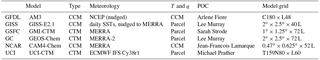
The six global chemistry models here are basically the same as those in P2017: Geophysical Fluid Dynamics Laboratory (GFDL), Goddard Institute for Space Studies (GISS), Goddard Space Flight Center (GSFC), GEOS-Chem (GC), National Center for Atmospheric Research (NCAR), and UC Irvine (UCI). For model versions and updates, see Tables 1 and S1a, b in the Supplement.
A model-simulated data stream of air parcels was prepared from an older version of the UCI model (v72a) with higher than usual resolution (T319L60, ∼ 0.55∘) and sampled at 00:00 UT 15 August 2005 at aircraft flight levels along three meridians next to 180∘ E. All the model grid cells are used with no attempt to follow ATom profiling. This set of 14 880 points is similar in number to 10 s data from an aircraft mission logging 50 flight hours in the Pacific basin, such as each seasonal deployment of ATom. Prescribed species are: O3, NOx (= NO + NO2), HNO3, HNO4, PAN (peroxyacetyl nitrate), RNO3 (CH3NO3 and all alkyl nitrates), HOOH, ROOH (CH3OOH and smaller contribution from C2H5OOH), HCHO, CH3CHO (acetaldehyde), C3H6O (acetone), CO, CH4, C2H6, alkanes (all C3H8 and higher), alkenes (all C2H4 and higher), aromatics (benzene, toluene, xylene), C5H8 (isoprene plus terpenes), plus temperature (T) and specific humidity (q). Zonal mean latitude by pressure plots of O3, CO, HCHO, NOx, PAN and q are shown in Fig. S1 in the Supplement.
The implementation of this data stream of reactive species is model dependent. All models begin with their own 3-D initialization data set that is used to restart a model simulation beginning on 16 August. The specified air-parcel NOx, for example, will be initialized as separate NO and NO2 abundances by scaling the model's restart values for NO and NO2 to match the specified parcel NOx. Similarly, a single value for aromatics will be partitioned over benzene, toluene, and xylene by models that resolve these species in accord with the restart values. The models place each parcel (i.e., overwrite the restart values) in the grid cell containing the latitude, longitude, and pressure specified for that parcel. If that preferred grid cell is already occupied with an air parcel, then an alternate adjacent grid cell is selected. It is recommended that alternate cells be shifted to minimize the change in photolytic environment (e.g., shift by longitude but maintain surface albedo and atmospheric mass). Two chemistry-climate models (GFDL, NCAR) were unable to completely overwrite the modeled T and q values with data stream values (see sensitivity tests below). See also Supplement for additional details.
Implications for reactivities are discussed below. It is difficult, if not impossible, to specify 24 h cloud fields, from observations or a model, in a way that all models here could implement consistently. Treatment of photolysis rates in uniform cloud layers is still quite different across models, and fractional overlapping cloud fields are often ignored, (e.g., Prather, 2015). Likewise, we do not attempt to control the profiles of O3 and aerosol above and below the air parcels insofar as they impact photolysis. Hence we diagnose photolysis rates (J-values) in addition to reactivities.
An inherent uncertainty is the day-to-day variability of clouds experienced by each parcel. Thus for the single data stream, each model calculates reactivities using the same chemical initialization but beginning with 5 different days in August: 1, 6, 11, 16, and 21. This 5-day variance gives us a measure of the uncertainty due to cloud variability, is similar across models, and thus provides a lower limit on the detection of model–model differences, i.e., a measure of “as good as it gets” in this comparison.
Several uncertainties are not answered with the standard protocol of 5-day runs: models ran with different calendar years and so how do 5-day means vary from year to year? Does the changing solar declination matter? Will different restart files (affecting O3 and aerosol profiles) alter the results? What if the 24 h integrations began at midnight rather than noon? How different are the CCMs because they use their own T and q for the parcels? The UCI CTM ran additional sensitivity calculations to address these questions, see Sect. 3.5 and figures in the Supplement.
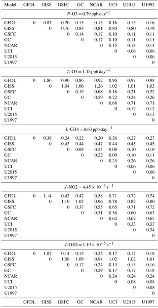
The difference in modeled reactivities for each parcel combines variations in cloud fields with basic differences in the chemical models (i.e., chemical mechanisms, numerical methods, photolysis treatment of cloudy and clear sky). The 5-day means reduce the effect of cloud variations but leave the fundamental differences in the photochemical modules, both photolytic and kinetic reactions. Our comparison looks at the parcel by parcel differences including the scatter (root mean square ,rms, differences) and average values across the models. To provide a standard for comparisons, we seek a reference case based on several models, and this is easily identified with the rms differences across all model pairs in Table 2). UCI ran 3 different model years to estimate the rms value caused by interannual variability (blue in Table 2), i.e., when the cross-model differences approach this value, we can accept that the photochemical modules including clouds cannot be said to be different in this study. For the reactivities (P-O3, L-O3, L-CH4), none of the cross-model pairs reached this lower limit, but certain groupings were consistently close, within a factor of 2 of this limit. For L-O3 and L-CH4, any pair of GSFC-GC-UCI fall within this range, while GFDL, GISS and NCAR are a factor of 5–10 above it. For the two CCMs this is likely caused by their use of different T and q's, while for GISS it probably lies in the chemical model. For P-O3, only the pair GC-UCI is within a factor of 2, but GFDL-GSFC-GC-UCI form a distinct cluster. The J-values, J-O1D (O3+ hv = > O2+ O(1D)) and J-NO2 (NO2+ hv = > NO + O), show groupings similar to this cluster, reflecting their common use of Fast-J versions (Wild et al., 2000; Prather, 2015), although this is unlikely to explain their similarity in P-O3.
Based on the average of the 5-day parcel means, we find a cluster of 3 similar models and three independent models. We need to find a common reference case against which to plot and statistically evaluate the models. Rather than pick one model, we take the 3-model average, GSFC-GC-UCI, as our reference. This clustering may be due to similar heritage: GSFC and GC are derived from a common tropospheric chemistry module; all three models and GISS have a common heritage for photolysis module. In the comparisons below, we will use terms like “bias” to describe differences with respect to this reference model. Such biases are not meant to be model errors since we do not know the correct answer; they are just model–model differences.
Table 2RMS differences of 5-day mean parcels across model pairs.
3.1 Average profiles
Altitude profiles of reactivities and J-values averaged over 24 h, 5 days in August, and latitude blocks (50–20∘ S, 20∘ S–20∘ N and 20–50∘ N) are shown in Fig. 1 (6 models, 3 blocks, 18 profiles per panel). As expected for August, the 50–20∘ S values are very low, while the 20∘ S–20∘ N and 20–50∘ N ones are equally high. This basic latitude-season pattern holds across all models. The variability across the five separate days in the UCI model (Fig. S2) is primarily a smooth trend through August reflecting the changing solar declination from 18∘ to 12∘, but instances of highly variable cloud fields occur, even when averaged over 30∘ in latitude.
For J-O1D, five models (GFDL, GSFC, GC, NCAR, UCI) agree well over all pressures and latitude blocks, but NCAR is, unusually, 10 % higher only in the 20∘ S–20∘ N block. J-O1D from GISS is 80 % larger than other models for all pressure and latitude blocks, but this does not translate directly or simply into reactivities, where GISS L-O3 is higher (expected) but L-CH4 is lower (unexpected). For J-NO2, model differences are not so great and show largest values at 20–50∘ N consistent with the longer summer daytime hours. The spread in J-NO2 is partly understandable because of ambiguous choices in interpolating the temperature dependence of recommended NO2 cross sections and quantum yields (i.e., the absorption cross sections are given at 220 and 294 K; the quantum yields, at 248 and 298 K; and the choice of whether to interpolate linearly or logarithmically, or whether to extrapolate or not, affects J-NO2, especially in the upper troposphere). This ambiguity does not exist for J-O1D recommended cross section and quantum yields. J-O1D is strongly dependent on the overhead O3 column, and the zonal mean total O3 column from the models is compared with recent satellite measurements in Fig. S3. NCAR's O3 column is anomalously lower only in the 20∘ S–20∘ N region and likely explains their higher J-O1D noted above.
Reactivity profiles for the five non-GISS models show excellent agreement for P-O3 but noticeable differences for L-CH4 and even larger ones for L-O3 (Fig. 1). The altitude profiles are similar for the five models, indicating that the cause of the L-O3 spread is likely related to HOX. The GISS results are anomalous, with much higher P-O3 and an L-O3 vs. L-CH4 relationship that seems counter to known chemistry in which both L-O3 and L-CH4 maximize with the high HOX values in the warmer, wetter, lower troposphere of the tropical Pacific.

Figure 1Different models' profiles of reactivities (P-O3; L-O3; L-CH4; all ppb day−1) and photolysis rates (J-NO2; J-O1D; all s−1) calculated for the data stream of 14 880 air parcels. Models are identified by color (black, GFDL; red, GISS; blue, GSFC; green, GC; magenta, NCAR; cyan, UCI). Latitude bands are identified by line style (solid, 20∘ S–20∘ N; dotted, 50–20∘ S; dashed, 20–50∘ N). Averages are over the five simulated dates in August, and all parcels are weighted equally.
3.2 14 880 parcels
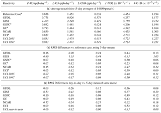
We examine the relationship between the three reactivities in each model with scatter plots of P-O3 and L-CH4 against L-O3 in Fig. 2. Each plot has 14 880 points (5-day parcel means) and is split by location: 60–20∘ S and 20–60∘ N (extra tropics, gray); tropics upper (20∘ S–20∘N, p < 600 hPa, cyan) and lower (p > 600 hPa, blue). Percentiles (10th, 50th, 90th) in each dimension are plotted as red dash-dot lines, and thus most points in the well correlated L-CH4 vs. L-O3 lie along the 3 quasi-diagonal intersections of red lines. The right-angle separation of high P-O3 and high L-O3 in the tropics reflects the high NOx (P-O3) in this data stream is in the upper troposphere and the largest L-O3 is from wet environments of the lower troposphere. GFDL has the most compact distribution of parcels and GISS, the most scattered. Four models (GSFC, GC, NCAR, UCI) have remarkably similar patterns in terms of the percentiles and structure, e.g., for L-CH4 vs. L-O3 they show the lower tropics dominating the upper part of the distribution and the extra-tropics, the lowermost points. GFDL has similar percentiles for P-O3 and L-CH4, but a much smaller spread for L-O3 that explains their compacted scatter plots. GISS is unique with much larger spread in both P-O3 and L-O3 but a compressed distribution in L-CH4. From these scatter plots, we can say that the four models are remarkably consistent, that GFDL is similar but should reexamine their L-O3 diagnostic, and that GISS has a “uniqueness” in its L-O3 vs. L-CH4 relationship as well as large scatter in both P-O3 and L-O3. While consistency does not guarantee correct implementation of the photochemical model (i.e., rate coefficients, cross sections), uniqueness is something that needs more investigation as it may be an error or may lead to fixes in the “consistent” models. Scatter plots of J-NO2 and J-O1D vs. L-O3 (Fig. S4) show similar J-value statistics for the five non-GISS models, and all models show a similar location of the three sets of points (extra-tropics, lower-tropics, upper-tropics) within their own percentiles.
On a parcel by parcel basis we compare in Fig. 3 the 5-day means from all six models against the reference case for the three reactivities and two J-values. If the models were all alike, they would fall tightly on the 1 : 1 line (black dashed). In each panel there are 89 280 points, with many overlapping. The order of plotting (shown by the legend) is important for visual impression since the latter points often overlie the earlier ones and the choice of order was based partly on the rms differences, with greatest first and smallest last. Here we can clearly see the type of scatter, the pattern of discrepancies across models, and at what levels of reactivity such discrepancy it occurs. It provides a focus for model development: UCI should reexamine its J-NO2 at the higher values and its P-O3 in the 1–3 ppb day−1 range; NCAR should examine why it has so much scatter in L-O3 and L-CH4 (see discussion of T and q later); GFDL has similar scatter (see T and q) but also has a low-bias in L-O3; and GISS has many differences that can be examined. As a cross-model question, are the above-the-line (UCI) and below-the-line (GSFC) differences in P-O3 and L-CH4 related to the same pattern in J-NO2?
Table 3Average reactivities and standard deviations with respect to the reference case (average of three models).
A simple summary of these statistics – averages and rms differences relative to the reference case – is given in Table 3. We have selected (italics) those entries that seem anomalous as also found in Fig. 3. For example, average P-O3 ranges from 0.77 to 0.84 ppb day−1 for five models but is 1.40 ppb day−1 for GISS. Likewise, average L-O3 ranges from 1.44 to 1.54 ppb day−1 for 4 models, but is 0.83 for GFDL and 2.25 ppb day−1 for GISS. The rms differences with respect to the reference case favors the three models that define that case, but also shows that GFDL and NCAR are close to the reference case for P-O3, but farther away for L-O3 and L-CH4 probably caused by their T and q values (see later).
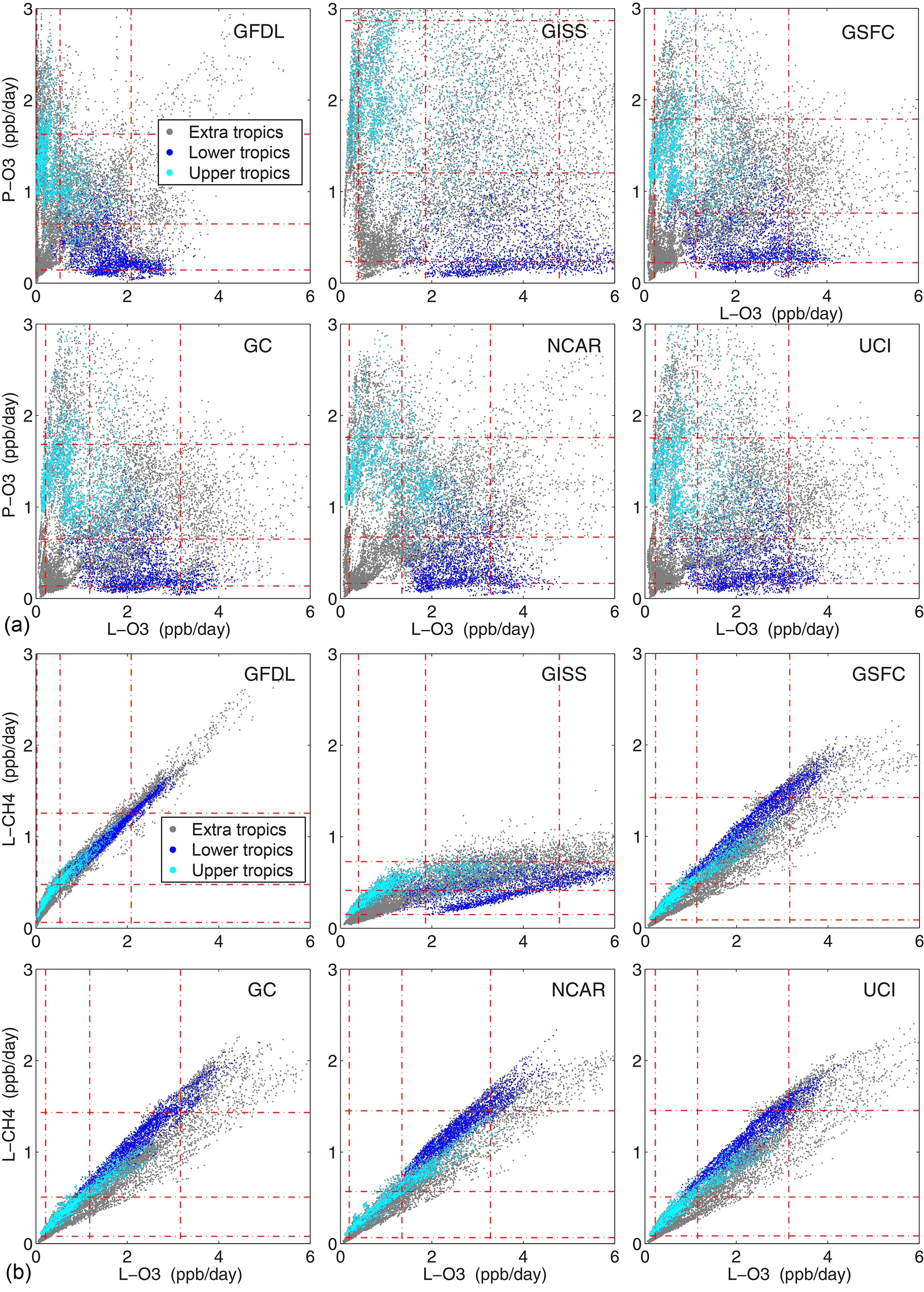
Figure 2Parcel reactivities of (a) P-O3 and (b) L-CH4 vs. L-O3 for each of the models. Points are colored by location: 60–20∘ S and 20–60∘ N (extra tropics, gray); tropics (20∘ S–20∘ N) upper (p < 600 hPa, cyan) and lower (p > 600 hPa, blue). The 10th, 50th, and 90th percentiles in each dimension are plotted as red dash-dot lines.

Figure 3Direct parcel by parcel comparison of modeled reactivities (a, P-O3; b, L-O3; c, L-CH4; all ppb day−1) and photolysis rates (d, J-NO2; e, J-O1D; all s−1) calculated for the 14 880 simulated air parcels. Each point is an average over the five simulated dates in August (01/8, 06/8, 11/8, 16/8, 21/8). The 1 : 1 line is shown (black dashed) for each plot. The reference values (x axis) are the average of three similar models (GSFC, GC, UCI) selected by examining the rms differences across all the models (see text). For this plot alone, models are plotted in the following order with the most disperse points being first for visibility: NCAR, GFDL, GISS, GC, UCI. GSFC. The model colors throughout this paper are consistent, but the order of plotting is shown in the legend.
3.3 Five days vs. 5-day mean
The variability of the five days in August tells us about the synoptic variability of clouds and possibly O3 columns in each model. The rms difference between the five individual days and the 5-day mean for each model (Table 3c) shows that GISS and NCAR have much larger variability in reactivities, caused by and mirrored by those in J-values. These rms differences in J-values for GISS and NCAR are surprising. Collectively, we should reexamine this variability in all the models to ascertain its cause. In general, the slopes of the individual vs. reference model for reactivities are close to 1 (Table S2) because the slope is determined by the large gradients with latitude and pressure that most models agree on. In comparing individual days vs. 5-day mean, it is encouraging that this slope averages 1 ± 0.04 for all reactivities and models (using each model's 5-day mean as its reference case, Table S3). Also, the slope decreases from about 1.01 to 0.96 through August as expected with declining photolysis rates in the north.
The rms difference across the five days is also a measure of how well the 5-day parcel mean can represent the true chemical model. Assuming that the cloud variability is random, the 5-day means with respect to other models are not really different unless that model–model rms exceeds some fraction of the day-to-day rms of the models involved. Using the UCI test with different model years, we find that the year-to-year rms differences are about two thirds of the day-to-day rms over 5-days. Thus, we cannot be sure that the rms differences between NCAR and the reference case are due to the inadequacy of the 5-day mean to represent the mean NCAR chemistry model (Table 3b, c). Conversely, some other source of model error is likely responsible for the large day-to-day rms.
3.4 The “hot” air parcels
Following the “which air matters” theme of P2017, we look at the more reactive air parcels to find out if the models agree on these. For each reactivity, we sort the 5-day parcel means in increasing order and integrate the cumulative reactivity. The value at 100 % (all 14 880 parcels) is equal to the average reactivity of the sample (Table 3a), and this is renormalized to 1 for comparison across models (Fig. 4, Table S4). With sorting, these curves must be monotonic and convex. The steeper the curve, the more important the top reactive parcels are in determining the total. For most models, these reactivity curves are remarkably similar and fall within the range seen for five different days with the same model (UCI, Fig. S5, Table S5). Focusing on the upper 10 %, the outliers are unusual and reactivity specific: for L-O3, GFDL is much steeper that the other models, consistent with the feature identified earlier in the scatter plots; and for L-CH4, GISS is much shallower. Surprisingly, with this diagnostic GISS is not an obvious outlier for P-O3 and L-O3 as seen in previous comparisons.
From this cumulative reactivity figure, one can see that the top 5 % of parcels comprise 15 % of the total reactivity, effectively a slope of 3 : 1. With the exceptions noted, total reactivity for the top 5, 10, 25, and 50 % of the parcels (Table S4) is similar across models and across days within a model (Table S5). Focusing on the top 10 % of parcels for each reactivity, we plot their latitude-by-pressure distribution for each model in Fig. 5. Top P-O3 are in the upper troposphere where NOx was highest in the specified data stream; and top L-O3 and L-CH4 are in the lower troposphere associated with warmer temperatures and higher water vapor, with L-CH4 being at lower altitude than L-O3 (all models except GISS). There is a region of top P-O3 parcels about 40∘ N that extends into the lower troposphere, although the shape varies across models. The vertical pattern of top-10 % parcels about 22∘ S clearly varies across models with GISS-GC-UCI not selecting these parcels.
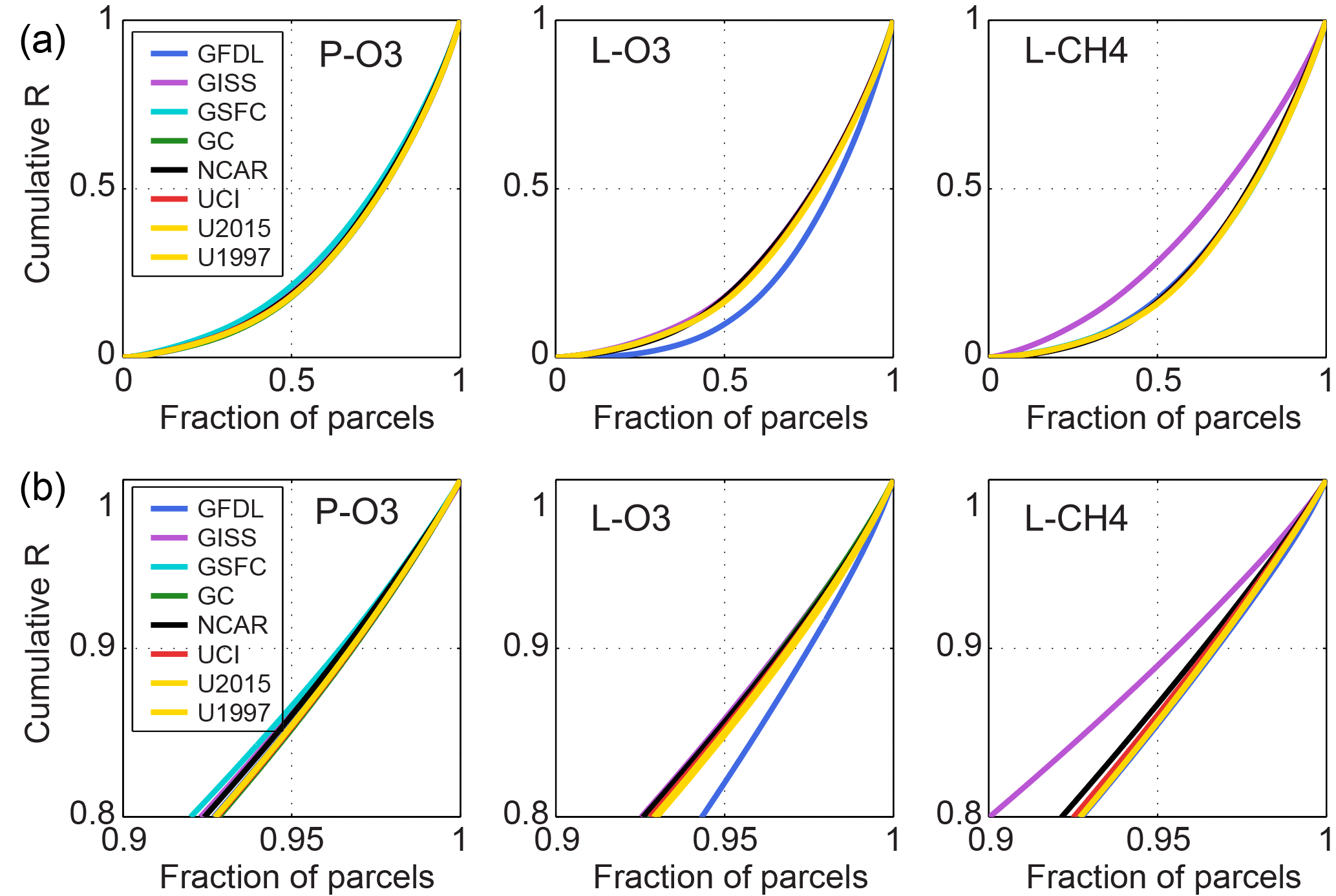
Figure 4Cumulative reactivity of the 14 880 parcels (equally weighted) scaled to the average of each model and reactivity. The lower panel shows a blowup of the top 20 % (Cumulative = 0.8 to 1.0). Results for the 6 models plus two different years for UCI are shown.

Figure 5Latitude (degrees) by pressure (hPa) location of the top 10 % of reactive parcels for the six models: P-O3 (red, large circles); L-O3 (blue, medium); L-CH4 (green, small).
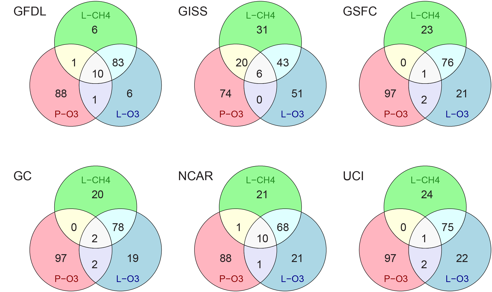
Figure 6Venn diagrams for each model showing the overlap (%) of the top 10 % parcels in each reactivity, using 5-day means for each parcel.
Overlap of these three sets of parcels are quantified as Venn diagrams for each model in Fig. 6. Very few top-10 parcels are in the triple-overlap area (1–10 %); but when P-O3 parcels coincide with either L-O3 or L-CH4 parcels, they generally lie in this triple-overlap area. The only major exception to this pattern is GISS. In terms of L-O3 and L-CH4 overlap, 4 models are very consistent (76–80 %); but GISS is unusually low (49 %) and GFDL is unusually high (93 %). These patterns help identify distinctly different chemistries in these models that have been identified with other diagnostics. The Venn overlap diagrams will become more interesting with an observational data stream as they point to the co-occurrence of unusual atmospheric parcels.
At what level do the models agree on the hot, top-10 % parcels? We use the reference case defined above and sort each reactivity to identify the top-10 %, retain those parcel numbers and compare across models. Table S6 gives each model's overlap of their top-X % parcels in terms of the percent that also occur in the top-X % reference case. For a range of X, 5, 10, 25, and 50 %, the overlap increases successively with many models having 90 % overlap for the top-50 %. The exceptions are GFDL with lower than typical overlap for L-O3 at all top-X % levels, and GISS, with lower overlap for L-CH4. This new diagnostic is helpful in understanding these model differences because it implies that the L-O3 and L-CH4 differences identified previously are not caused by a systematic offset in all parcels, but rather by a selection of different parcels.
As expected, the three models GSFC-GC-UCI that define the reference case all have about 90 % overlap for the top-10 % parcels, and so we do not learn much with this. In terms of linking models with similar chemistries, probably 80 % overlap is a good mark, because we see that the different UCI years drop off to 85 % in L-O3 and L-CH4. Overlap in P-O3 is much easier to achieve as the few high-NOx parcels drive high P-O3 in all models: at the top-25 % parcels, the P-O3 overlap is about 84 % or better for all models.
On a day-to-day basis, we examine the top-10 % overlap for GC–GSFC–NCAR–UCI models, using their own 5-day mean as the reference (Table S7). Cloud variations across the five days lead to overlaps for the top-10 % parcels ranging from 78 to 92 % at best. NCAR has similar self-overlaps for P-O3 but only 58 to 72 % for L-O3 and L-CH4, because the modeled T and q changes with each day in August and greatly reduces the overlap of the hot parcels. This further supports T and q as being important drivers of L-O3 and L-CH4. The use of 5-day calculations with varying cloud fields is essential in identifying the top reactive parcels.
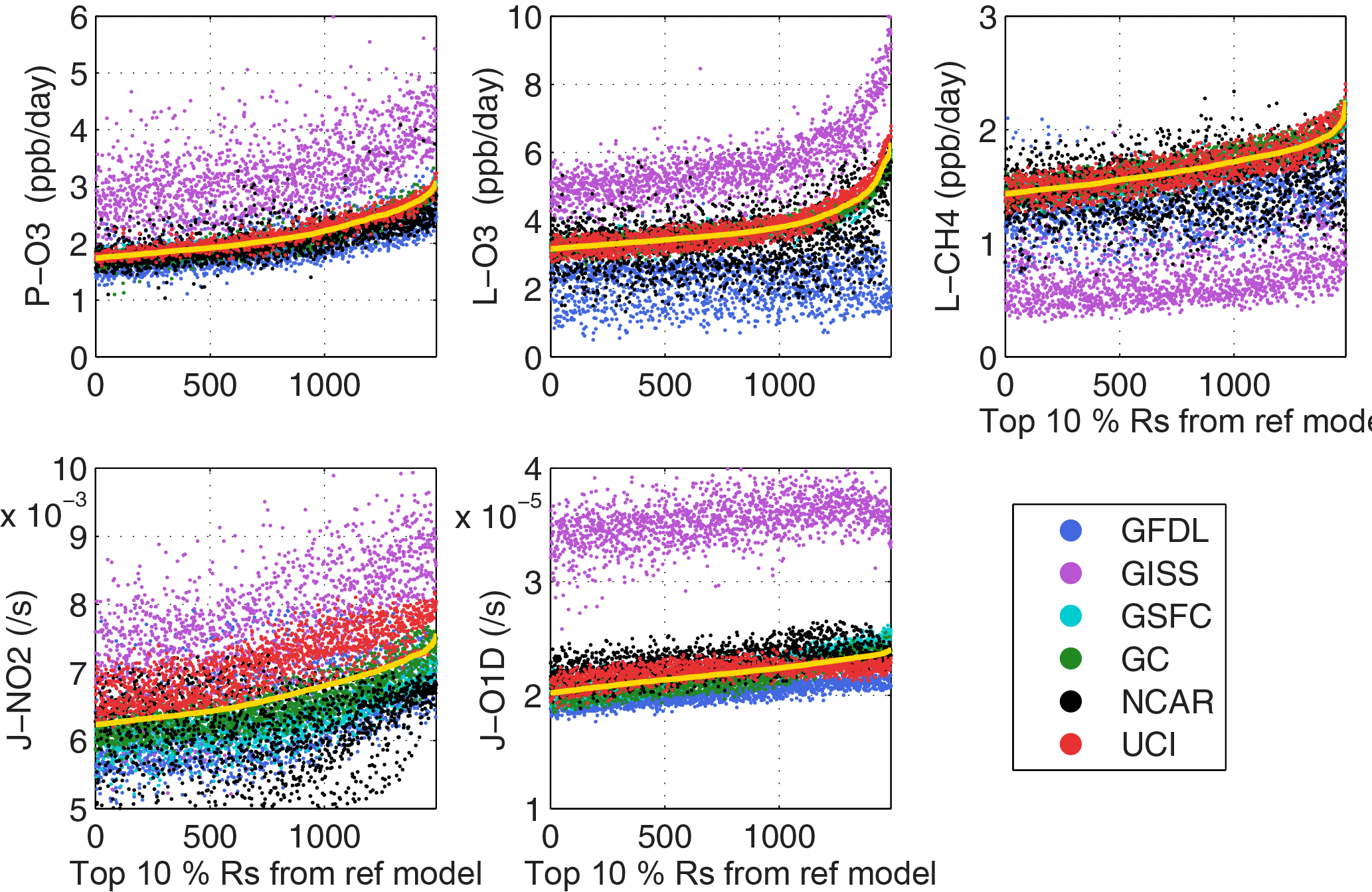
Figure 7Modeled Reactivity and J-values for 5-day mean parcels plotted using the top-10 % in the reference case in ascending order along the x axis. The black dashed monotonically increasing line is the reference case parcels.
We plot the modeled reactivity of individual model 5-day mean parcels in ascending order based on the sorted top-10 % parcels in the reference case (Fig. 7). Hence the reference case (black line) is a monotonically increasing curve; while the individual models produce a scattered distribution of points. As expected, the three models defining the reference case have some scatter but mostly overlap with the reference case. UCI is typically higher and GSFC is lower. For J-NO2 in these most reactive parcels, UCI is notably higher as is GISS, a result seen in the average profiles (Fig. 1), but it does not affect the reactivities. The mean bias of models relative to the reference case is also seen in Fig. 7 with the offset of the points. The results here are similar to what has been identified earlier: GISS has unusual offsets for all reactivities and J-O1D; agreement for P-O3 is much better than for L-O3 and L-CH4; four models show the upward curve matching the top-1 % parcels; for L-O3 and L-CH4, GFDL-NCAR have a flat scatter of points and miss the upward curve because they reset the q of the data stream. Day-to-day scatter for the top-10 % (defined by the 5-day mean) is tested with the UCI model in Fig. S6. This one-model synoptic cloud variability has similar scatter to that seen for the more central models (Fig. 7) including the rapid increase in L-O3 at the top-1 % and the much greater scatter in J-NO2. The year-to-year variability in the top-10 % parcels is shown (Fig. S7) for the UCI model with year 2016 as the reference case (solid line) and years 1997 and 2015 as separate models. The patterns of scatter here are similar to but less than the day-to-day (Fig. S6), again showing the importance of 5-day averages, and identifying the lower limit of scatter at which this diagnostic can discern differences in model chemistry. Overall, the top-10 % J-O1D parcels (all in uppermost troposphere) have better agreement than the top-10 % J-NO2 which are more sensitive to clouds.
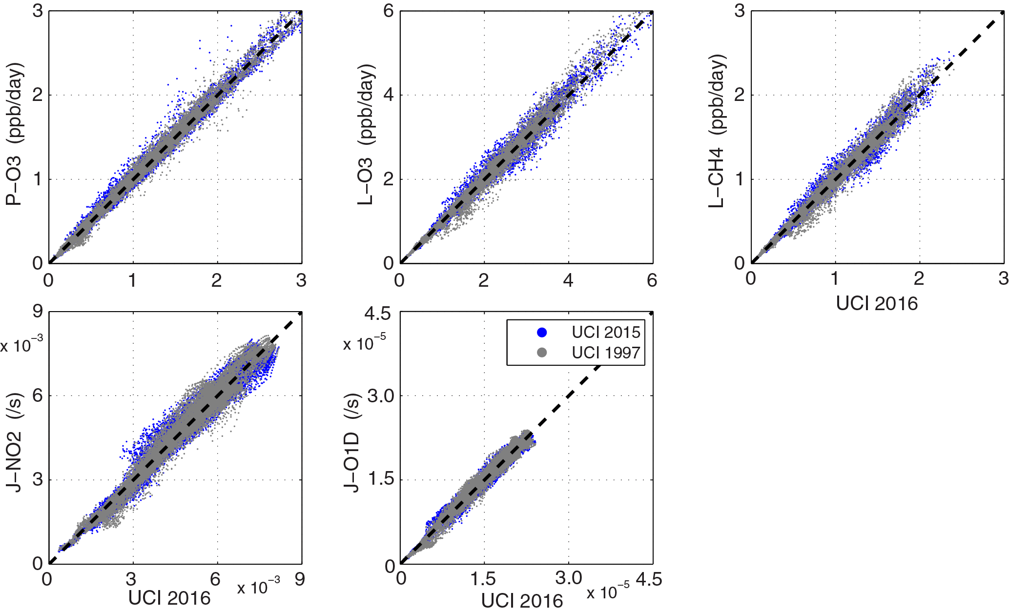
Figure 8Scatter plot of reactivities and J-values for 5d-mean air parcels for UCI alternate meteorological years (2015, 1997) against the standard year 2016.
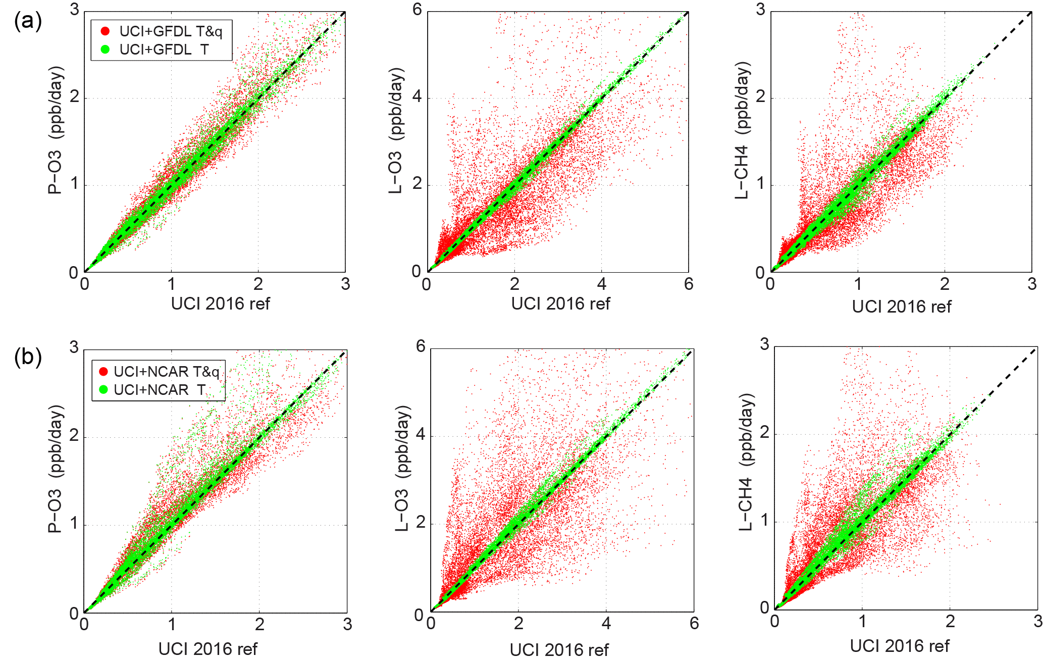
Figure 9Scatter plot of reactivities of the 14 880 air parcels showing the effect of the GFDL (a) and NCAR (b) models using T and q from their climate models, instead of from the specified data stream. The UCI model for a single day (16 August 2016) calculated reactivities using the GFDL and NCAR parcel values for T alone (green) and for T and q (red) and compared with the UCI reference model for 16 August 2016.
3.5 Assumptions and uncertainties in the experiment design
How interannual variability might affect the results is tested with the UCI CTM running the simulated data stream for five August days using years 1997 and 2015 meteorology to compare with year 2016 (see previous Tables, Table S8, and Fig. 8). The scatter plots in Fig. 8 do not look much different from those for the three models used in the reference case (Fig. 3). For the 5-day parcel means, the rms differences across any pairing of the three UCI years is about 8–10 % of the average reactivity, which is about half of that across the three models used in the reference case. Using this criterion (< 20 %) for distinctness, we effectively have only four independent distinctly different models here: GFDL, GISS, NCAR and the GSFC–GC–UCI group. The four models all differ from one another at the 30–100 % level of the UCI year-to-year variations. However, in terms of the overall average reactivities (Table 3), the different years of the UCI model are almost identical (< 1 %), while the differences across the three reference models are much larger (±5 %) and clearly distinguishable.
How the time-of-day of parcels in the data stream might affect reactivity is tested with the UCI model initializing the calculation at midnight (12:00 UT) instead of noon (see Fig. S8, Table S8). In this study, we chose parcels at 180∘ W and, since the global models begin each day at 00:00 UT, the photochemistry starts at local noon. A measurement data stream, such as from ATom (2017), will include measurements over a range of longitudes and taken with a wide range of local solar times. We need to ensure that the protocol here does not depend on when the 24 h integration of reactivity is initiated. The UCI model selected one day (16 August 2016) and shifted the local solar time by 12 h, thus initiating each parcel at local midnight. In addition, the cloud fields needed to be rearranged so that the pairing of clouds and solar zenith angles were the same in both cases. The start-at-midnight version has larger reactivities by at most 1 % with no changes in the J-values as expected for the protocol (e.g., keeping the morning clouds in the morning for both calculations). The rms differences between the two cases are 2–10 times less than the year-to-year differences. We conclude that the initiation time produces discernible differences but not at the level to affect the any of the results here, even with high levels of lightning-NO in daytime. The initiation time might affect highly polluted regions where the NOx reservoirs could be converted at night to less photolabile nitrates.
Two additional sensitivity tests included running the five days in August with a fixed solar declination (Fig. S9) and with different restart file (Fig. S10). As shown in these figures and Table S8, these two tests change the overall average in the fourth decimal place and have rms differences < 0.01 ppb day−1. For these choices, the protocol adopted here is adequate.
The GFDL and NCAR CCMs could not maintain the fixed, data-stream T and q values over the 24 h integration, which leads to larger rms differences because reactivities depend on both T and q. This explains in part why the GFDL and NCAR models in Fig. 3 have larger scatter for reactivities than the other non-GISS models, but similar scatter in J-values. This effect may also contribute to the larger day-to-day rms, for NCAR at least, and is examined more extensively with the UCI CTM running with the T and q's from both models (Sect. 3.5).
How overwriting of the data stream's T and q (with a CCM climate) impacts these results is tested with the UCI CTM re-running a one day (16 August 2016) data stream using T and q's reported from the GFDL and NCAR models. The rms reactivity differences for these two models are 2–3 times larger than those of the reference models (GSFC, GC, UCI, see Table 3); while J-value differences (much less affected by temperature) are similar.
For the five days, each with 14 880 parcels, the mean values of either GFDL or NCAR T and q's are similar to the data stream but their rms differences are large: about 3.6∘ K and 0.4 in log10(q), see Table S9. Both models have similar scatter patterns for T and for q (Fig. S11) with a number of parcels having log10(q) more than a factor of 10 different from the stream. In this sensitivity test, UCI CTM ran with just T from GFDL and NCAR, and then with both T and q (4 cases in all). The results are shown in Tables S8 and Fig. 9. For T alone, the reactivity differences were at the lower limit of detectable model–model differences but, with both T and q, the model showed surprisingly large shifts in L-O3 and L-CH4 along with standard deviations 2–10 times larger than the lower limit based on different UCI model years. In fact, the UCI model using GFDL and NCAR T and q has about the same rms reactivity differences with respect to the reference case as do the full models (Compare Tables S8 and 3, noting that Table 3 is a 5-day mean result and not 1-day result). Thus, without a model being able to use the specified T and q, we are unable to determine if its photochemical module is similar to another model. Moreover, with climate-varying T and q's the modeled reactivities from an observed data stream will also be too noisy for an analysis of the top-10 % parcels, i.e., which air matters.
We develop a new protocol for merging in situ measurements with 3-D model simulations of atmospheric chemistry as calculated by chemistry-transport models through to Earth system models. The goal is to take a time stream of species-rich, high-resolution (100–300 m), spatially sparse observations, such as from an aircraft mission (e.g., ATom, 2017), and have the current 3-D global or regional models use that observed data directly to evaluate chemical reactivity in each parcel. With this protocol, we avoid model artifacts in the data stream, such as occur in assimilated data, but must account for the density and bias in sampling. Here, we focus on tropospheric production and loss of the greenhouse gases ozone and methane, but the protocol can be readily applied to other chemical transformations such as the formation and growth of secondary organic aerosols.
In applying the protocol here to a synthetic data stream, we demonstrate a second major use: detailed diagnostics of model performance, specific to the photochemical modules operating within the global chemistry-climate and chemistry-transport models. Six such models are evaluated here, and their differences and similarities in simulating the chemistry are clearly identified. The protocol specifies the detailed chemical composition of a constrained set of air parcels including temperature and water vapor, embeds these parcels in an appropriate grid cell of each model, turns off processes that mix adjacent grid cells, and integrates the 3-D model for 24 h (see P2017). The photochemical module is thus dependent only on the chemical mechanism and the diurnal cycle of photolysis rates, which are driven in turn by temperature, water vapor, solar zenith angle, clouds, possibly aerosols and overhead ozone, which are calculated as they would be in each model.
Typical 3-D multi-model evaluations cannot separate differences in photochemistry from differences in emissions, transport, scavenging, and even numerical methods, all of which help define the mix of chemical species in each grid cell. The new protocol established in this paper combines the no-transport A-run from P2017 with the data stream of specified-composition air parcels. The approach is generic and can be implemented in any model. Here, using six global chemistry-transport or chemistry-climate models, we can see how it opens a window focusing specifically on the photochemical modules embedded in 3-D models.
Overall, the models show surprisingly good agreement on calculating the reactivity (P-O3, L-O3, L-CH4) and photolysis rates (J-NO2, J-O1D) in air parcels. We can identify unique features in each model: e.g., UCI's high J-NO2 values; GSFC's lower P-O3 at high reactivity; GISS's inverted results for L-O3 vs. L-CH4; GFDL and NCAR's large scatter due to use of model-generated vs. parcel-specified water vapor; and large variability in J-values for NCAR and GISS. Models with effectively the same chemistry module will appear distinct if they use a different data stream for water vapor. It is impossible to tell if overall, among the six models, GISS has the most unique features, and GC the least. These anomalous features can really only be explained by the model developers who understand the coding, yet these diagnostics point to a focus for the analysis of individual models. Being a standout in any diagnostic, does not necessarily imply that uniqueness is an error, but it should encourage self-evaluation to determine if that unique feature is intentional and can be shown to be a more accurate simulation.
Cloud variations on synoptic scales are primary sources of noise in this study. These are difficult to standardize from either model or observation, given the wide range of methods for treating cloud scattering and overlap. Cloud-driven changes in reactivity are clear in comparisons across models and also within the same model. Use of a single day for comparison is inadequate. This protocol selects five days across the month to sample cloud fields, and this provides a stable average for identifying model–model difference. The protocol also makes several simplifying assumptions that may affect results: the solar declination over the month is fixed at the mid-month value; and the 24 h integration is always started globally at the same universal time, meaning at different local solar times across the longitudes. These issues were tested with a single model and found to be unimportant compared with the synoptic variability in clouds and other model–model differences.
Using day-to-day and year-to-year variability in a single model, we can define a lower limit to the differences, which is essentially the noise in this protocol, such that models are not distinguishably different. For the most part, we find that the GSFC, GC and UCI models fall into this “indistinguishable from one another” class because their differences are within a factor of 2 of the estimated noise level. This grouping may be explained in part by the common heritage of GSFC and GC's tropospheric chemical model, but UCI's chemical mechanism is completely different and much abbreviated. All other model pairings show much larger differences.
All models agree that the more highly reactive parcels dominate the chemistry; for example, the hottest 10 % of parcels control 25–30 % of the total reactivities. Unfortunately, they do not agree on which parcels comprise the top 10 %. This diagnostic will become more acute as we move from the smoothed synthetic data stream derived from model output (50 × 50 × 1 km averages) to the high variability of in situ ATom observations (2 × 2 × ∼ 0.1 km averages).
Based on our experience comparing models that differ largely by temperature and water vapor, we conclude that water vapor differences in CCM simulations of past and future atmospheres may be a major cause of the changes in O3 and CH4 and may lead to different chemistry-climate feedbacks across the models.
This new protocol for multi-model evaluations helps identify and provide insights into inter-model differences, as well as providing for a direct link with measurements made at a much finer scale than the models.
The merged ATom data stream is now at the Oak Ridge National Laboratory DAAC (https://doi.org/10.3334/ORNLDAAC/1581) (Wofsy et al., 2018), and these model data and results are also available at Prather et al. (2018) at https://doi.org/10.3334/ORNLDAAC/1597.
The supplement related to this article is available online at: https://doi.org/10.5194/amt-11-2653-2018-supplement.
The authors declare that they have no conflict of interest.
This work was supported by the ATom investigation under National
Aeronautics and Space Administration's Earth Venture program (grants
NNX15AJ23G, NNX15AG57A). We thank Jingqiu Mao and Larry Horowitz for
assistance with GFDL AM3, and Drew Shindell for assistance with GISS model
2E.
Edited by: Ronald Cohen
Reviewed by: two anonymous referees
ATom: Measurements and modeling results from the NASA Atmospheric Tomography Mission, available at: https://espoarchive.nasa.gov/archive/browse/atom (last access: 30 April 2018), 2017.
Batchelor, G. K.: The Effect of Homogeneous Turbulence on Material Lines and Surfaces, Proc. R. Soc. Lon. Ser.-A, 213, 349–366, https://doi.org/10.1098/rspa.1952.0130, 1952.
Collins, W. J., Lamarque, J.-F., Schulz, M., Boucher, O., Eyring, V., Hegglin, M. I., Maycock, A., Myhre, G., Prather, M., Shindell, D., and Smith, S. J.: AerChemMIP: quantifying the effects of chemistry and aerosols in CMIP6, Geosci. Model Dev., 10, 585–607, https://doi.org/10.5194/gmd-10-585-2017, 2017.
Eyring, V., Butchart, N., Waugh, D. W., Akiyoshi, H., Austin, J., Bekki, S., Bodeker, G. E., Boville, B. A., Brühl, C., Chipperfield, M. P., Cordero, E., Dameris, M., Deushi, M., Fioletov, V. E., Frith, S. M., Garcia, R. R., Gettelman, A., Giorgetta, M. A., Grewe, V., Jourdain, L., Kinnison, D. E., Mancini, E., Marchand, M., Marsh, D. R., Nagashima, T., Newman, P. A., Nielsen, J. E., Pawson, S., Pitari, G., Plummer, D. A., Rozanov, E., Schraner, M., Shepherd, T. G., Shibata, K., Stolarski, R. S., Struthers, H., Tian, W., and Yoshiki, M.: Assessment of temperature, trace species, and ozone in chemistry-climate model simulations of the recent past, J. Geophys. Res.-Atmos., 111, D22308, https://doi.org/10.1029/2006jd007327, 2006.
Lauritzen, P. H., Ullrich, P. A., Jablonowski, C., Bosler, P. A., Calhoun, D., Conley, A. J., Enomoto, T., Dong, L., Dubey, S., Guba, O., Hansen, A. B., Kaas, E., Kent, J., Lamarque, J.-F., Prather, M. J., Reinert, D., Shashkin, V. V., Skamarock, W. C., Sørensen, B., Taylor, M. A., and Tolstykh, M. A.: A standard test case suite for two-dimensional linear transport on the sphere: results from a collection of state-of-the-art schemes, Geosci. Model Dev., 7, 105–145, https://doi.org/10.5194/gmd-7-105-2014, 2014.
Morgenstern, O., Hegglin, M. I., Rozanov, E., O'Connor, F. M., Abraham, N. L., Akiyoshi, H., Archibald, A. T., Bekki, S., Butchart, N., Chipperfield, M. P., Deushi, M., Dhomse, S. S., Garcia, R. R., Hardiman, S. C., Horowitz, L. W., Jöckel, P., Josse, B., Kinnison, D., Lin, M., Mancini, E., Manyin, M. E., Marchand, M., Marécal, V., Michou, M., Oman, L. D., Pitari, G., Plummer, D. A., Revell, L. E., Saint-Martin, D., Schofield, R., Stenke, A., Stone, K., Sudo, K., Tanaka, T. Y., Tilmes, S., Yamashita, Y., Yoshida, K., and Zeng, G.: Review of the global models used within phase 1 of the Chemistry–Climate Model Initiative (CCMI), Geosci. Model Dev., 10, 639–671, https://doi.org/10.5194/gmd-10-639-2017, 2017.
Myhre, G., Aas, W., Cherian, R., Collins, W., Faluvegi, G., Flanner, M., Forster, P., Hodnebrog, Ø., Klimont, Z., Lund, M. T., Mülmenstädt, J., Lund Myhre, C., Olivié, D., Prather, M., Quaas, J., Samset, B. H., Schnell, J. L., Schulz, M., Shindell, D., Skeie, R. B., Takemura, T., and Tsyro, S.: Multi-model simulations of aerosol and ozone radiative forcing due to anthropogenic emission changes during the period 1990–2015, Atmos. Chem. Phys., 17, 2709–2720, https://doi.org/10.5194/acp-17-2709-2017, 2017.
NAP: Causes and Effects of Changes in Stratospheric Ozone: Update 1983, ISBN 0-309-03443-4, National Academy Press, Washington D.C., USA, 1984.
NASA: Report of the 1992 Stratospheric Models and Measurements Workshop, edited by: Prather, M. J. and Remsberg, E. E.), Satellite Beach, FL, USA, February 1992, NASA Ref. Publ. 1292, 144 + 268 + 352 pp., 1993.
Nault, B. A., Garland, C., Wooldridge, P. J., Brune, W. H., Campuzano-Jost, P., Crounse, J. D., Day, D. A., Dibb, J., Hall, S. R., Huey, L. G., Jimenez, J. L., Liu, X. X., Mao, J. Q., Mikoviny, T., Peischl, J., Pollack, I. B., Ren, X. R., Ryerson, T. B., Scheuer, E., Ullmann, K., Wennberg, P. O., Wisthaler, A., Zhang, L., and Cohen, R. C.: Observational Constraints on the Oxidation of NOx in the Upper Troposphere, J. Phys. Chem. A, 120, 1468–1478, https://doi.org/10.1021/acs.jpca.5b07824, 2016.
Olson, J., Prather, M., Berntsen, T., Carmichael, G., Chatfield, R., Connell, P., Derwent, R., Horowitz, L., Jin, S. X., Kanakidou, M., Kasibhatla, P., Kotamarthi, R., Kuhn, M., Law, K., Penner, J., Perliski, L., Sillman, S., Stordal, F., Thompson, A., and Wild, O.: Results from the Intergovernmental Panel on Climatic Change Photochemical Model Intercomparison (PhotoComp), J. Geophys. Res.-Atmos., 102, 5979–5991, 1997.
Olson, J. R., Crawford, J. H., Brune, W., Mao, J., Ren, X., Fried, A., Anderson, B., Apel, E., Beaver, M., Blake, D., Chen, G., Crounse, J., Dibb, J., Diskin, G., Hall, S. R., Huey, L. G., Knapp, D., Richter, D., Riemer, D., Clair, J. St., Ullmann, K., Walega, J., Weibring, P., Weinheimer, A., Wennberg, P., and Wisthaler, A.: An analysis of fast photochemistry over high northern latitudes during spring and summer using in-situ observations from ARCTAS and TOPSE, Atmos. Chem. Phys., 12, 6799–6825, https://doi.org/10.5194/acp-12-6799-2012, 2012.
Orbe, C., Waugh, D. W., Newman, P. A., and Steenrod, S.: The Transit-Time Distribution from the Northern Hemisphere Midlatitude Surface, J. Atmos. Sci., 73, 3785–3802, https://doi.org/10.1175/Jas-D-15-0289.1, 2016.
PhotoComp: Chapter 6 – Stratospheric Chemistry SPARC Report No. 5 on the Evaluation of Chemistry-Climate Models, World Meteorological Organization, Geneva, Switzerland, 194–202, 2010.
Prather, M. and Jaffe, A. H.: Global Impact of the Antarctic Ozone Hole – Chemical Propagation, J. Geophys. Res.-Atmos., 95, 3473–3492, 1990.
Prather, M., Flynn, C., Fiore, A., Correa, G., Strode, S. A., Steenrod, S., Murray, L., and Lamarque, J.-F.: ATom: Simulated Data Stream for Modeling ATom-like Measurements. ORNL DAAC, Oak Ridge, Tennessee, USA, available at: https://doi.org/10.3334/ORNLDAAC/1597, last access: 1 May 2018.
Prather, M. J., Zhu, X., Strahan, S. E., Steenrod, S. D., and Rodriguez, J. M.: Quantifying errors in trace species transport modeling, P. Natl. Acad. Sci. USA, 105, 19617–19621, https://doi.org/10.1073/pnas.0806541106, 2008.
Prather, M. J.: Photolysis rates in correlated overlapping cloud fields: Cloud-J 7.3c, Geosci. Model Dev., 8, 2587–2595, https://doi.org/10.5194/gmd-8-2587-2015, 2015.
Prather, M. J., Zhu, X., Flynn, C. M., Strode, S. A., Rodriguez, J. M., Steenrod, S. D., Liu, J., Lamarque, J.-F., Fiore, A. M., Horowitz, L. W., Mao, J., Murray, L. T., Shindell, D. T., and Wofsy, S. C.: Global atmospheric chemistry – which air matters, Atmos. Chem. Phys., 17, 9081–9102, https://doi.org/10.5194/acp-17-9081-2017, 2017.
Shindell, D., Kuylenstierna, J. C. I., Vignati, E., van Dingenen, R., Amann, M., Klimont, Z., Anenberg, S. C., Muller, N., Janssens-Maenhout, G., Raes, F., Schwartz, J., Faluvegi, G., Pozzoli, L., Kupiainen, K., Hoglund-Isaksson, L., Emberson, L., Streets, D., Ramanathan, V., Hicks, K., Oanh, N. T. K., Milly, G., Williams, M., Demkine, V., and Fowler, D.: Simultaneously Mitigating Near-Term Climate Change and Improving Human Health and Food Security, Science, 335, 183–189, https://doi.org/10.1126/science.1210026, 2012.
Wild, O., Zhu, X., and Prather, M. J.: Fast-J: Accurate simulation of in- and below-cloud photolysis in tropospheric chemical models, J. Atmos. Chem., 37, 245–282, 2000.
Wofsy, S. C., Apel, E., Blake, D. R., Brock, C. A., Brune, W. H., Bui, T. P., Daube, B. C., Dibb, J. E., Diskin, G. S., Elkiins, J. W., Froyd, K., Hall, S. R., Hanisco, T. F., Huey, L. G., Jimenez, J. L., McKain, K., Montzka, S. A., Ryerson, T. B., Schwarz, J. P., Stephens, B. B., Weinzierl, B., and Wennberg, P.: ATom: Merged Atmospheric Chemistry, Trace Gases, and Aerosols. ORNL DAAC, Oak Ridge, Tennessee, USA, available at: https://doi.org/10.3334/ORNLDAAC/1581, last access: 30 April 2018.