the Creative Commons Attribution 4.0 License.
the Creative Commons Attribution 4.0 License.
 | 18 May 2018
Derivation of gravity wave intrinsic parameters and vertical wavelength using a single scanning OH(3-1) airglow spectrometer
Thomas Offenwanger
Carsten Schmidt
Michael Bittner
Christoph Jacobi
Gunter Stober
Jeng-Hwa Yee
Martin G. Mlynczak
James M. Russell III
For the first time, we present an approach to derive zonal, meridional, and vertical wavelengths as well as periods of gravity waves based on only one OH* spectrometer, addressing one vibrational-rotational transition. Knowledge of these parameters is a precondition for the calculation of further information, such as the wave group velocity vector.
OH(3-1) spectrometer measurements allow the analysis of gravity wave ground-based periods but spatial information cannot necessarily be deduced. We use a scanning spectrometer and harmonic analysis to derive horizontal wavelengths at the mesopause altitude above Oberpfaffenhofen (48.09∘ N, 11.28∘ E), Germany for 22 nights in 2015. Based on the approximation of the dispersion relation for gravity waves of low and medium frequencies and additional horizontal wind information, we calculate vertical wavelengths. The mesopause wind measurements nearest to Oberpfaffenhofen are conducted at Collm (51.30∘ N, 13.02∘ E), Germany, ca. 380 km northeast of Oberpfaffenhofen, by a meteor radar.
In order to compare our results, vertical temperature profiles of TIMED-SABER (thermosphere ionosphere mesosphere energetics dynamics, sounding of the atmosphere using broadband emission radiometry) overpasses are analysed with respect to the dominating vertical wavelength.
- Article
(3752 KB) - Full-text XML
- BibTeX
- EndNote


In order to analyse atmospheric motions like gravity waves, the upper mesosphere and lower thermosphere is studied by a variety of measurement techniques: airglow spectroscopy and imaging, as well as lidar systems, are probably the most prominent ones in the Network for the Detection of Mesospheric Change (NDMC, https://www.wdc.dlr.de/ndmc).
Depending on the instrument and the retrieval, different techniques are sensitive to different wave parameters. While lidar measurements, for example, allow the measurement of vertical wavelengths (see, e.g. Rauthe et al., 2006, 2008; Yamashita et al., 2009; Mzé et al., 2014; Chen et al., 2016), horizontal wavelengths of gravity waves can be directly extracted from airglow images (for instance, Garcia et al., 1997; Taylor et al., 2003; Paulino et al., 2011). OH-airglow spectroscopy and typical meteor radar measurements deliver gravity wave periods (e.g. Mulligan et al., 1995; Bittner et al., 2000; Hocking, 2001; Oleynikov et al., 2005).
Further wave parameters can be calculated if additional information is available, which allows the application of the dispersion relation. Also, the instrument setup can be changed in order to compute further wave parameters.
Wachter et al. (2015) show that the combination of three airglow spectrometers measuring different azimuth angles allows the derivation of horizontal wavelengths. Due to the setup of the three instruments, their fields of view (FoVs) and the data analysis technique, the retrieved wavelengths lie mostly in the range of a few hundred kilometres, the addressed wave periods range from 1 to 14 h, with a maximum number of waves between 2 and 4 h. Small-scale horizontal features in the order of some kilometres to a few hundred metre or even turbulent structures, which are observed with OH* cameras as shown by Sedlak et al. (2016) and Hannawald et al. (2016), cannot be investigated based on this approach.
Schmidt et al. (2017) introduced a method to derive vertical wavelengths from OH* spectrometer measurements by observing two vibrational transitions, OH(3-1) and OH(4-2). Following the work of von Savigny (2012), the radiation emitted by the different vibrational transitions originates from slightly different heights, which are separated by a few 100 m. For approximately 40 % of the wave events, a vertical wavelength can be derived which lies in the range of 5–40 km. Of course, the same approach can be applied to measurements of different airglow species peaking at different heights, for example, OH(6-2) and O2b(0-1), which are separated by ca. 7 km.
Here, we combine the approach of Wachter at al. (2015) in order to derive horizontal wavelengths (but based on only one OH* spectrometer) with additional information about the horizontal wind and the Brunt–Väisälä frequency and compute vertical wavelengths. Thus, every component of the wave vector is known. This is a precondition for the calculation of further information like the wave group velocity vector or the vertical flux of horizontal wave pseudo-momentum, for example (see e.g. Fritts and Alexander, 2003). However, the derivation of these values is beyond the scope of this manuscript.
The wave vector is related to the intrinsic wave frequency, i.e. the frequency that would be observed in a frame of reference moving with the horizontal background wind, via the Brunt–Väisälä frequency and the Coriolis parameter (dispersion equation, see Eq. 38 in Fritts and Alexander, 2003). Based on the work of Wachter et al. (2015), we constructed a scanning OH* spectrometer (Sect. 2.1) which allows the derivation of periods and zonal as well as meridional wavelengths (method: Sect. 3.1, and results: Sect. 4.1). We then use literature values of the Brunt–Väisälä frequency (see e.g. Wüst et al., 2016, 2017b) and the nearest mesopause wind measurements, which are performed by a meteor radar (Sect. 2.3) in order to estimate the vertical wavelengths (method: Sect. 3.1, and results: Sect. 4.2). The scanning spectrometer operates at Oberpfaffenhofen (48.09∘ N, 11.28∘ E), Germany, the meteor radar is deployed at Collm (51.30∘ N, 13.02∘ E), Germany, ca. 380 km northeast of Oberpfaffenhofen; therefore, specific focus is put on a thorough uncertainty estimation (Sect. 3.2). Finally, the results are compared to vertical wavelengths extracted from collocated TIMED-SABER temperature profiles (Sects. 2.2, and 4.2).
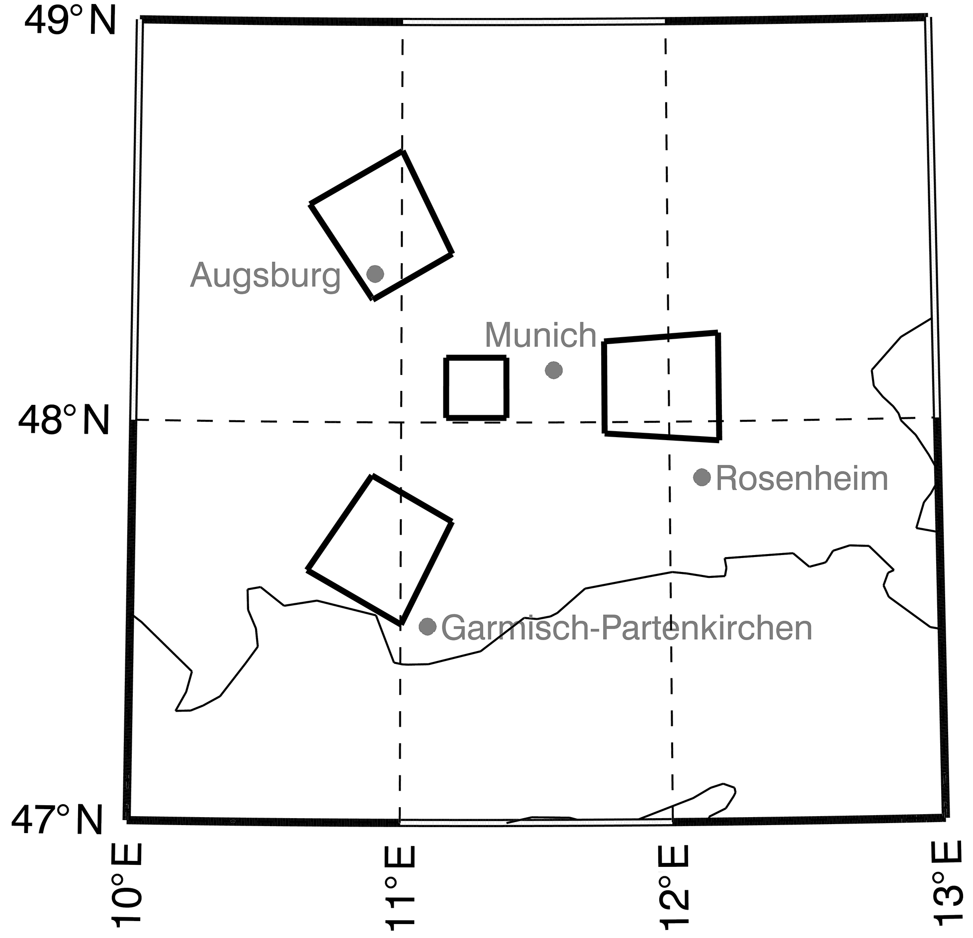
Figure 1The scanning GRIPS points in four different directions. The FoV in the zenith direction is the smallest one with an edge length of 23–24 km at the mesopause height resulting in a covered area of ca. 560 km2. The remaining three FoVs are larger (approximately 880 km2). All four FoVs together form an equilateral triangle, whose sides are approximately 90 km long.
2.1 Infrared spectrometer GRIPS
The nightly airglow observations presented here are performed with the scanning infrared spectrometer GRIPS 14 (Ground based Infrared P-branch Spectrometer) at Oberpfaffenhofen (48.09∘ N, 11.28∘ E), Germany, July–November 2015. The instrument operates in the spectral range of 1.5 to 1.6 µm. Therefore, observations are only possible under (nearly) cloudless conditions. They address a height of ca. 86 km (e.g. Wüst et al., 2016, 2017b).
Concerning its basic components and its data processing, GRIPS 14 is identical to the GRIPS instruments described by Schmidt et al. (2013). The technical layout of the scanning mirror is designed to result in three FoVs forming an equilateral triangle (zenith angles: 30∘) in the mesopause region with the fourth FoV being in the centre of the triangle, in the zenith direction. The edge length of the FoV triangle amounts to 90 km. Due to the finite aperture of the GRIPS 14, each FoV covers approximately 880 km2, excluding the one in the zenith direction. The latter is smaller with approximately 560 km2 (see Fig. 1). The instrument acquires spectra with a temporal resolution of 15 s. Thus, it is possible to get airglow spectra from four FoVs in approximately one minute.
The rotational temperature derived from an individual spectrum can typically exhibit an uncertainty of ±8 K. In order to improve the signal-to-noise ratio for the intended analysis, 5 min mean values are calculated for each FoV. Only comparatively good individual values are used here (individual error 4.5 K and less as in Wüst et al., 2016). The error of the 5-minute values reaches ca. 3.2 K on average with a standard deviation of 0.3 K. Additional care has been taken to ensure that the data quality of each FoV is comparable to the others by manually inspecting each night: due to the geographic location of Oberpfaffenhofen, just north of the Alps, clouds frequently form predominantly in the southern FoV or the moon passes through one of the FoVs. These cases are excluded from further analysis.
2.2 TIMED-SABER
On 7 December 2001, the TIMED satellite was launched. Soon, the on-board limb-sounder SABER started to deliver vertical profiles of kinetic temperature on a routine basis. The profiles cover the height range from approximately 10 km to more than 100 km. The vertical resolution is ca. 2 km (Mertens et al., 2004; Mlynczak, 1997), which is suitable for the investigation of gravity wave activity. On a given day, the latitudinal coverage extends from about 52∘ latitude in one hemisphere to 83∘ in the other (Russell et al., 1999). This viewing geometry alternates once every 60 days due to 180∘ yaw manoeuvres of the TIMED satellite (Russell et al., 1999). In total, approximately 1200 temperature profiles are available per day. An overview of the large number of SABER publications is available at http://saber.gats-inc.com/publications.php.
Measurements of infrared emission from carbon dioxide in the 15 µm spectral interval are used in the SABER temperature retrieval. It is based on a comprehensive forward radiance model incorporating dozens of vibration-rotation bands of CO2, including isotopic and hot bands, and solving the full set of coupled radiative transfer equations under non-LTE, i.e. under conditions that depart from local thermodynamic equilibrium. From the temperature retrieval version 1.03 on, NLTE algorithms for kinetic temperature were employed (López-Puertas et al., 2004; Mertens et al., 2004, 2008). This is certainly one of the main challenges for CO2 based temperature retrievals in the mesosphere and upper levels. Comparisons with reference data sets generally confirm good quality of SABER temperatures (Remsberg et al., 2008).
We use nightly TIMED-SABER temperature data between 45.4 and 50.8∘ N and 8.6 and 14.0∘ E (∼ 300 km distance from Oberpfaffenhofen (48.09∘ N, 11.28∘ N)) in its latest version (2.0). They were downloaded from the SABER homepage (http://saber.gats-inc.com). The exact time can be looked up in Table 1. Only SABER profiles that were measured at the same time as GRIPS data series were used.
The data were detrended between 100 km and their height minimum using an iterative cubic spline approach as it is described in Wüst et al. (2017a) with a distance of 10 km between two spline sampling points. This results in a maximal detectable wavelength of 20 km (in the detrended data series). We restrict further analysis to a relatively small height interval of 60–80 km which is just below the height range addressed by GRIPS. This is due to the following reasons. Especially during summer (May–August), a time period which is also covered in this study, the mesopause is low and reaches ca. 86 km ± 3 km (von Zahn et al., 1996; She et al., 2000). Sharply changing temperature gradients are always a challenge for a de-trending procedure and artificial signals in the detrended data cannot be excluded here. This is the reason why we investigate only heights below 80 km with the harmonic analysis. The majority of commonly used spectral analysis techniques like the fast fourier transform, the maximum entropy method and also the harmonic analysis approach, all assume the waves are stationary and therefore a constant wave amplitude. Alternative analyses suited for non-stationary time series like, the wavelet analysis, for example, often suffer from a relatively coarse spectral resolution. Therefore, we restrict our analysis to the smallest possible height interval which is equal to the maximal wavelength detectable in the detrended data series.
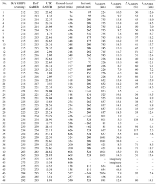
Table 1Ground-based period T, intrinsic frequency σ, vertical and horizontal wavelengths, λz and λh, as well as error of the vertical wavelength Δλz, derived from GRIPS, and vertical wavelength λz (if calculated) derived from SABER measurements during different nights (DoY = day of year when the measurement started), and date as well as time of the co-located SABER measurements.
2.3 Meteor wind radar
The VHF SKiYMET meteor radar located at Collm has been operated nearly continuously since July 2004 (Jacobi et al., 2007, 2009). It measures winds, temperatures, and some meteor parameters at altitudes between approximately 80 and 100 km.
The radar operates at a frequency of 36.2 MHz, with 15 kW peak power at a pulse repetition frequency of 625 Hz. The transmit antenna is a crossed dipole one, while the 5 receiving antennas during 2015 were 2-element Yagi antennas, forming an interferometer to detect the meteor position.
The radar uses the Doppler shift of the reflected radio wave from ionized meteor trails to obtain radial velocities along the line of sight of the radio wave. Hourly mean horizontal wind values are obtained from a least squares fit of the projection of the horizontal hourly wind components to all individual radial winds within 1 h and within a defined height gate under the assumption that vertical winds are small. We used height gates of 4 km width for the fit, without weighting the individual meteors and assuming that the wind field within the time-height bin is homogeneous. Horizontal homogeneity of the horizontal wind field within the radar observation volume is also assumed. The procedure is described in Hocking et al. (2001). A more recent version of the wind fitting technique and error estimation of meteor radar winds can be found in Stober et al. (2017).
In order to estimate the error that arises from using the Collm observations for the wind field over Oberpfaffenhofen at a distance of about 380 km, we evaluated the differences of winds measured by the Collm radar and the 53.5 MHz OSWIN VHF radar (Latteck et al., 1999) at Kühlungsborn (54.1∘ N, 11.8∘ E), about 330 km distance from Collm, during a half-year campaign in 2004/05 (Viehweg, 2006). The OSWIN radar had been operated as a meteor radar (Singer at al., 2003), with the same analysis procedure than applied at Collm. The Collm–Kühlungsborn differences were increasing from −0.7 ± 22.3 m s−1 at 85 km to −2.5 ± 25.5 m s−1 at 94 km for the zonal component, and −0.1 ± 20.3 m s−1 at 85 km to −2.05 ± 24.9 m s−1 at 94 km for the meridional component. The small biases may be explained by the mean northward gradients of the horizontal winds, which at these heights in winter are positive for both the zonal and meridional wind components. The standard deviation is due to waves, turbulence, and uncertainties of both systems.
Therefore, when using Collm data for estimating winds over Oberpfaffenhofen, the standard deviation of about 20 m s−1 may be considered as a good guess for the dynamically induced wind differences.
3.1 Derivation of 3-D wave vector
The basic idea of the algorithm applied here for the calculation of horizontal wavelengths from a scanning GRIPS instrument is already mentioned in Wachter et al. (2015). In contrast to their publication, we derive OH-temperatures for four instead of three FoVs with one scanning GRIPS instrument instead of three individual (non-scanning) ones. Since three FoVs are sufficient for the calculation of horizontal wavelengths, we use the additional information for the estimation of uncertainty intervals.
We apply the harmonic analysis (all-step mode, see for example Bittner et al., 1994, or Wüst and Bittner, 2006) to the four nightly time series and search for four identical (ground-based, not intrinsic) periods throughout the entire night. Further analysis steps are restricted to results which are characterized by a period longer (shorter) than 60 min (the measurement time) and an amplitude larger than or equal to 1 K. This is in accordance with the approach and the results of Wachter et al. (2015) (see their Sect. 2.2).
Since four different triangles can be derived from four different FoVs, we apply the algorithm described in Wachter et al. (2015) to each possible triangle combination. So, we get information about the horizontal wavelengths λh(wave numbers kh) from each of the four triangle combinations for four waves at maximum. Zonal and meridional wavelengths (numbers) λx(k) and λy(l), phase velocities, and propagation directions can be derived. The mean parameters are calculated for each wave, and the mean absolute difference between the individual values and the mean parameters are taken as a measure of uncertainty.
Since phase velocities reported in the literature do not in most cases exceed 150 m s−1 (e.g. Nakamura et al., 1999; Taylor et al., 2009; Tang et al., 2014; Wachter et al., 2015), only waves with a mean phase velocity of 150 m s−1 at maximum and a mean horizontal wavelength of less than or equal to 3600 km are subject of further analysis. Additionally, a maximal difference of 90∘ between the four different wave vectors is accepted. It turned out that this criterion is the strictest one: if it is fulfilled, the others are met as well.
Going one step further than Wachter et al. (2015), we then use the dispersion relation for the estimation of vertical wavelengths. According to linear theory (see, for example, Fritts and Alexander, 2003), it holds the following:
where m is the vertical wave number, N is the Brunt–Väisälä frequency, is the intrinsic frequency (the frequency that would be observed in a frame of reference moving with the background wind ), ω is the frequency derived by the harmonic analysis, is the Coriolis parameter with respect to the latitude β, which reaches typically 10−4 s−1 for mid-latitudes, and H is the density scale height.
For low- and medium-frequency waves (σ∼f or the dispersion relation simplifies to the following:
where kh is the horizontal wave number (see Eq. 38 in Fritts and Alexander, 2003). The term can be neglected since it is small compared to the squared vertical wave number. Due to the selection criteria for frequency and horizontal wave numbers, ω, k, and l are rather small and the use of this approximation is justifiable.
Information about mesopause wind velocities above Oberpfaffenhofen is not available. Since tides, which are variable from day to day, play an important role in this height range, we do not rely on climatological wind values but make use of wind measurements performed with the wind meteor radar at Collm in order to estimate the intrinsic frequency.
Since GRIPS only measures the temperature at about 86 km height, but not the temperature gradient, the Brunt–Väisälä (angular) frequency is calculated based on the collocated TIMED-SABER measurements.
3.2 Error estimation
Since ω is calculated using four different time series and applying a variety of quality criteria, we argue that the error of ω is negligible. Following error propagation, the error of λz then sums up to the following:
with the following equations:
Following Wüst et al. (2016) and Wüst et al. (2017b), is ca. 10 %. This might be overestimated, since N is calculated from collocated TIMED-SABER profiles. However, the satellite-based measurements do not agree exactly in space with the GRIPS measurements. They represent only a snapshot and analyses concerning the general temporal and spatial variability of N within 300 km are difficult due to the distance of individual TIMED-SABER profiles. Δu and Δv are approximately 20 m s−1 (see Sect. 2.3), and Δk and Δl are estimated as stated above (see Sect. 3.1). Now, Δλz an be calculated.
Errors which may arise due to tidal effects on the OH-layer height are not considered here. Strong tidal perturbations lead to airglow-altitude changes from typically 2–7 km (Zhao et al., 2005). If all four FoVs are affected to the same extent (the OH-airglow altitude is shifted by a constant value), our results are not influenced. If the OH-airglow layer height increases or decreases for each FoV individually, the derived horizontal wavelengths can change. However, our results rely on spatial and temporal averages. The FoVs cover 880 km2 (560 km2); all values which we derive are averaged over this area. Furthermore, we analyse time series of 7 h and longer. So, effects of motions of these scales cancel out. The four FoVs are rather near to each other. This reduces the possible effect of large scale motions like tides on our analysis results tremendously. Due to the redundancy of the system (we get four values for the horizontal wavelength), we dismiss results which do not agree sufficiently (as mentioned in Sect. 3.1). This might be the case when not all but only one or two FoVs are influenced by a higher or lower airglow altitude.
There is a secondary tidal effect. If the OH-airglow layer height disagrees significantly from 86 km, we use the wind information of the wrong altitude bin. Due to the width of the altitude bins, we might be one bin off in the case of strong tidal perturbations as mentioned above. The error depends on the vertical wind shear. Placke et al. (2011) show histograms of the zonal and meridional wind shear values (prevailing and tidal wind) for the years 2005–2009 referring to July measured by the radar at Collm. On average, the zonal (meridional) wind shear is ca. 5 m s−1 km−1 (0 m s−1 km−1). So if we are one bin off, this is equivalent to 20 m s−1. This agrees with the error which we assumed for each wind component.

Figure 2The histogram of the horizontal wavelengths (a) shows that the majority of detected wave events reaches up to 1000 km. The distribution of phase velocities (relative to the ground) (b) is smoother and has a maximum between 20 and 40 m s−1. The diagram of horizontal propagation directions (c) does not show a conclusive picture. The different grey colours refer to the different months.
4.1 Horizontal parameters
Due to the rather strict quality criteria, horizontal wavelengths for 31 wave events in only 22 nights can be identified during the measurement period. For the majority of cases, the horizontal wavelength is shorter than 1000 km, with a maximum of the distribution between 600 and 800 km (Fig. 2a). The phase velocity (relative to the ground) reaches 140 m s−1 at maximum and ranges mostly between 20 and 40 m s−1 (Fig. 2b). A preferred propagation direction cannot easily be identified (Fig. 2c). The data cover the time period from July to November; since the propagation direction is supposed to show seasonal variations (see Wachter et al., 2015, and references therein) and our data base is rather small, a conclusive picture cannot be drawn here.
The values for the different parameters agree well with literature. Phase velocities up to 80–100 m s−1 are reported, for example, by Nakamura et al. (1999), Suzuki et al. (2004), and Taylor et al. (2009). For example, Tang et al. (2014) and Wachter et al. (2015) find horizontal phase speeds of up to 160–180 m s−1. The horizontal wavelengths cannot easily be compared since many authors focus on smaller horizontal scales (see, for example, Tang et al., 2014; Taylor et al., 2009; Hannawald et al., 2016; Sedlak et al., 2016). However, Reid (1986) presents in his Fig. 6a good overview of horizontal wavelengths measured by different techniques at various locations between 60 and 100 km height. Here, it becomes clear that horizontal wavelengths of the order of 103 km were already observed in earlier studies. However, in order to be careful, the results of the following subsection are separated according to the horizontal wavelength (up to 1500 km and all wavelengths, provided in brackets if the results disagree).
4.2 Vertical wavelengths
Vertical wavelengths derived from the scanning GRIPS are compared to vertical wavelengths extracted from TIMED-SABER temperature profiles. Therefore, we identify all nights with co-located TIMED-SABER measurements around Oberpfaffenhofen. Depending on the orbit of TIMED, it can happen that no vertical temperature profile is suitable for any given day. However, the on other days more than one profile may be available. In this case, multiple nearby SABER profiles, which may show different vertical wavelengths, can be used for comparison. Since the wind velocity changes considerably during the night, we calculate linearly weighted wind speeds from the hourly means of the wind data according to the overflight time of TIMED. If multiple nearby SABER profiles are available, the detected wave from the airglow is combined with different wind values. This leads to different vertical wavelengths based on the GRIPS-radar combination for one night. In one case, the respective hourly averaged wind data do not exist. Therefore, 19 horizontal wavelengths of the 31 mentioned in Sect. 4.1 referring to 14 of 22 nights can be used for further analysis. The data availability of TIMED-SABER and meteor wind measurements allows the calculation of 48 vertical wavelengths (see Table 2).
In three cases, the wavelengths are shorter than 2 km (no. 23, 30 and 32 in Table 1). This does not seem to be a realistic value for a layer with a full width at half maximum of 8–9 km (see Fig. 9 in Wüst et al., 2016, 2017b). Furthermore, as Trinh et al. (2015) show in their Fig. 7a, SABER is not sensitive for vertical wavelengths shorter than ∼ 2.5 km. In five cases (twice two nearly simultaneously measured SABER profiles), the wavelengths are rather long with ca. 38.0 km (no. 36 and 37 in Table 1), 45.9 km (no. 44 and 45 in Table 1) and 33.4 km (no. 47 in Table 1). This is in principle possible and was already observed in the past (see, for example, Manson, 1990, and Stober et al., 2013) but hard to verify here since we use SABER profiles only between 60 and 80 km – see Sect. 2.2 for an explanation. In two cases (two nearly simultaneously measured SABER profiles), the result is imaginary (no. 42 and 43 in Table 1), which means that the wave cannot propagate vertically. We cannot verify this case either. So, 38 cases (79 % of 48 vertical wavelengths) show reasonable and verifiable results.
The mean vertical wavelength derived by the combination of GRIPS and the meteor radar is 11.6 km (Fig. 3a). This agrees well with literature: Rauthe et al. (2008), for example, investigated vertical lidar temperature profiles between 1 and 105 km height recorded at Kühlungsborn (54.1∘ N, 11.8∘ E), which is located about 800 km north of Oberpfaffenhofen, with a wavelet analysis. In their Fig. 5b, they show the dominating vertical wavelength depending on month. For a maximum height of 80 km, it ranges between 13 and 15 km. Senft et al. (1991) report a similar finding for Urbana (40.1∘ N, 88.2∘ W), USA. Based on 60 nights of Na-lidar measurements, they find that characteristic vertical wavelengths vary between 8.9 and 27 km. The annual mean reaches 14.1 km if one refers only to summer values, it is 12.7 km, winter values show a mean of 15.5 km.
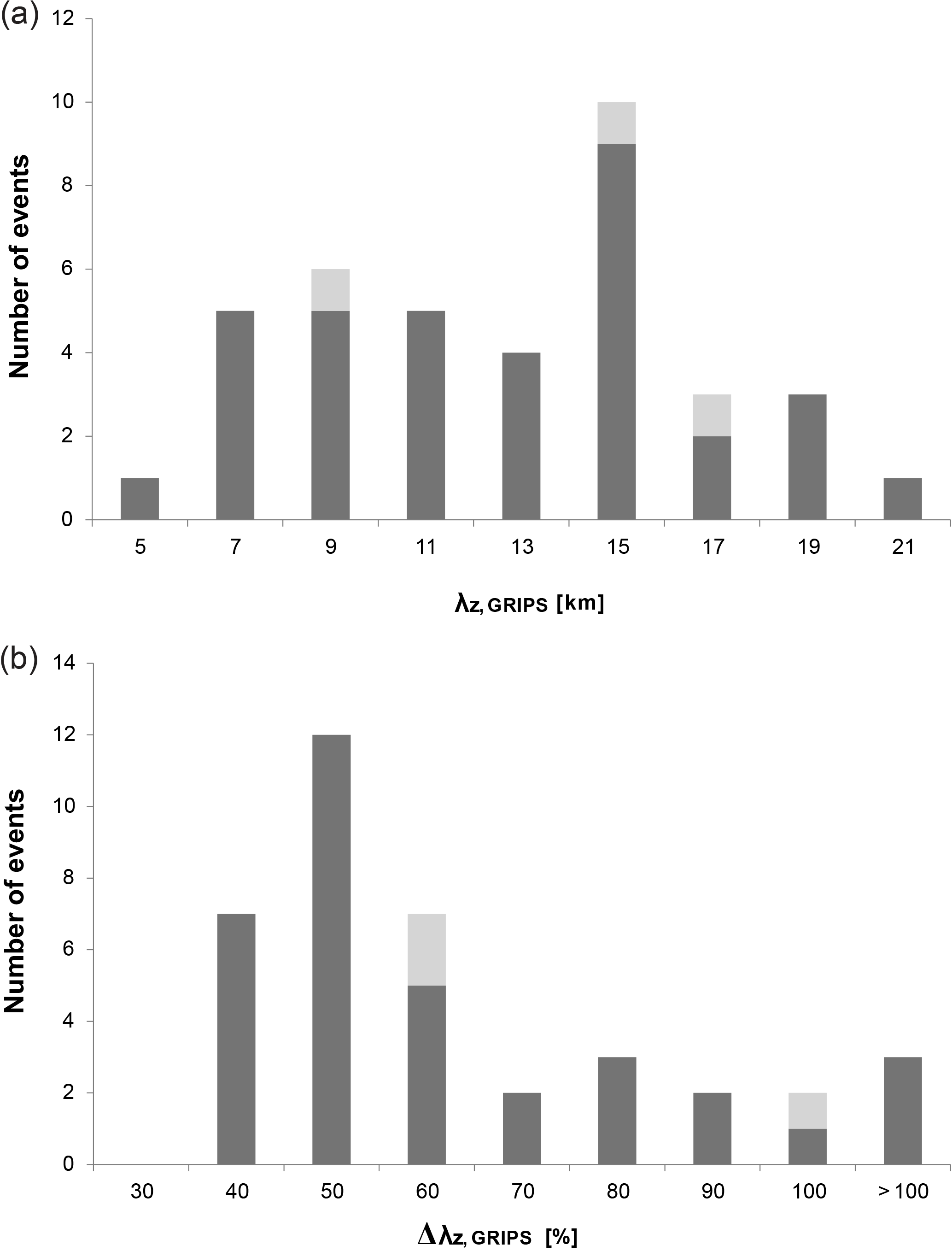
Figure 3The mean calculated vertical wavelength is ca. 11.6 km, while the individual values spread from 5 to 19–20 km (a), the x axis labels are the upper limits of the respective intervals. The mean error of the vertical wavelength Δλz based on error propagation calculations reaches ca. 59 % (b). At minimum, it ranges between 30 and 40 %; in three cases, it is more than 100 %. The values for the waves with horizontal wavelengths larger than 1500 km are marked in light grey.
The mean error following Eq. (3) sums up to 59 % (Fig. 3b). In nearly all cases, the largest contribution to the individual Δλz is due to the wind uncertainty (Eqs. 7 and 8).
In order to compare the vertical wavelengths derived by GRIPS with SABER measurements, the harmonic analysis is used for searching the detrended TIMED-SABER temperature profiles for two vertical wavelengths between 2.5 km (minimal vertical wavelengths detectable in SABER measurements according to Trinh et al., 2015) and 20 km (height interval length). Two wavelengths are chosen since an inspection shows at least two oscillations in the SABER profiles. The sensitivity of TIMED-SABER depends on the vertical and horizontal wavelength along the line of sight. For a wave with 12.5 km vertical wavelength, the horizontal wavelength (along the line of sight) needs to be 450 km at least, to ensure that SABER captures it with 50 % and more of its original amplitude (see Trinh et al., 2015, for example). The horizontal wavelength along the line of sight is always larger or equal to the true horizontal wavelength. The TIMED-SABER data are therefore suitable for our purpose (compare Fig. 2a).
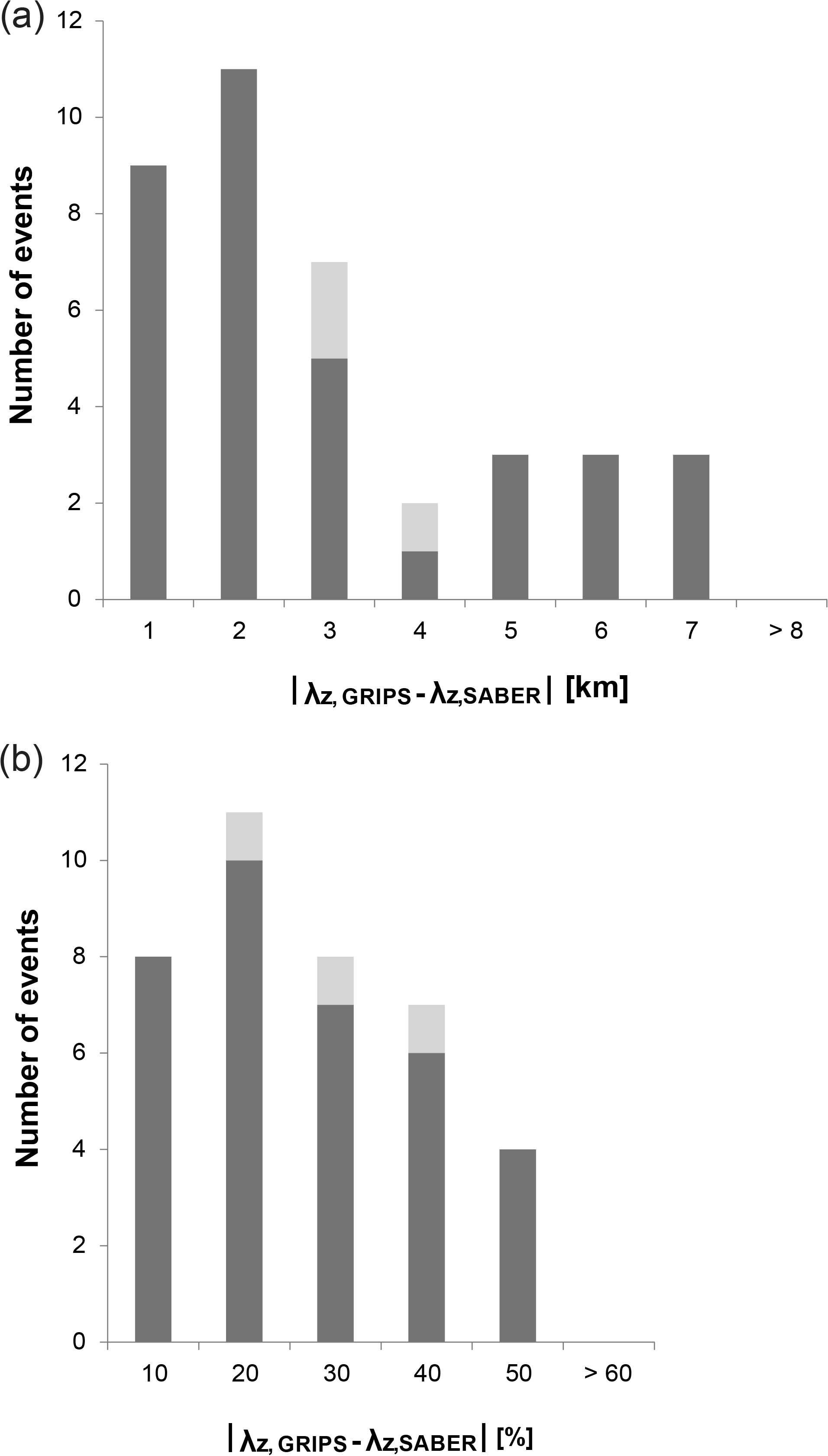
Figure 4The mean difference between the vertical wavelength derived by the scanning GRIPS λz,GRIPS and the most similar vertical wavelength identified in collocated TIMED-SABER vertical temperature profiles λz,SABER is ca. 2.5 km (a) or 21 % (b). It reaches 6–7 km or 40–50 % at maximum.
The two oscillations identified by the harmonic analysis explain ca. 81 % (80 %) of the TIMED-SABER temperature variability on average which can be judged as a good value. The oscillation which agrees best with the vertical wavelength derived from the GRIPS-radar combination is used for further comparison (this value is given in Table 1). The mean individual difference between the vertical wavelengths of both data sets then reaches ca. 2.5 km or 21 % relative to the GRIPS wavelength (Fig. 4a and b). The vertical wavelengths agree within the error bars in all but four cases; here, the vertical wavelengths derived from SABER are slightly smaller by 0.2–0.8 km.
We conclude that the presented approach provides reasonable results for the 3-D wave vector. However, the data basis is not very large. Like other measurement techniques or approaches, this one is also sensitive to certain horizontal and vertical wavelengths: the vertical extension of the OH*-layer limits the sensitivity of the GRIPS-instrument for vertical wavelengths to a few kilometres at least (see Wüst et al., 2016 for a comprehensive overview). The sensitivity for horizontal wavelengths is determined by the distance between the different FoVs (∼ 90 km here) and their sizes (see Wüst et al., 2016, for an estimation of this effect), as well as by the quality of the data, which strongly depends on the weather: only if a phase difference unequal to zero for the individual time series can be identified, the derivation of the horizontal wave vector and subsequently of the vertical wave number is possible.
Using a scanning OH-spectrometer at Oberpfaffenhofen (48.09∘ N, 11.28∘ E), Germany, we derive periods and horizontal wavelengths at the mesopause which are typical for gravity waves (ca. 1–10 h, 100–1000s km). Based on the dispersion relation, additional horizontal wind information allows the calculation of vertical wavelengths. The nearest mesopause wind measurements are carried out at Collm (51.30∘ N, 13.02∘ E), Germany, approximately 380 km northeast of Oberpfaffenhofen by a meteor radar. We assume that these values are also valid for Oberpfaffenhofen within an uncertainty of ±20 m s−1.
Ca. 79 % of the vertical wavelengths range between 5 km and 19–20 km. These values appear reasonable compared to literature and taking into account the vertical extension of the OH-layer. In three cases (ca. 6 %), the values are not plausible.
The results are compared to vertical wavelengths derived from collocated detrended TIMED-SABER measurements. Although the spectrometer and the meteor radar are deployed about 380 km apart from each other, the vertical wavelengths based on the spectrometer-radar data combination and the satellite data only show a mean difference of 2.5 km or 21 % (relative to the GRIPS wavelength). We conclude that the presented combination of measurements provides a good estimate of the vertical wavelengths on average.
The SABER data are available at the SABER homepage http://saber.gats-inc.com/data.php (SABER, 2018). The NDMC are available at https://doi.org/10.1594/WDCRSAT.R4OAR50I (Offenwanger et al., 2018). Collm hourly radar wind data are available from Christoph Jacobi upon request.
The authors declare that they have no conflict of interest.
We thank the Bavarian State Ministry of the Environment and Consumer Protection (BayStMinUV, VAO-project LUDWIG, TP I/3, project number TUS01 UFS-67093) and the German Ministry for Education and Research (BMBF, Grant agreement No: 01LG1206A) for funding.
Furthermore, we thank Ricarda Linz, formerly at DLR, for detrending the SABER data and Paul Wachter, DLR, for a preliminary setup of the scanning GRIPS-instrument.
Processing and long-term archiving of the data is provided by the World Data Center for Remote Sensing of the Atmosphere (WDC-RSAT, http://wdc.dlr.de). The measurements are part of the Network for the Detection of Mesospheric Change, NDMC (https://www.wdc.dlr.de/ndmc).
Finally, we thank the reviewers for their valuable comments.
The article processing charges for this open-access
publication were covered by a Research
Centre
of the Helmholtz Association.
Edited by:
William Ward
Reviewed by: Alan Liu and two anonymous referees
Bittner, M., Offermann, D., Bugaeva, I. V., Kokin, G. A., Koshelkov, J. P., Krivolutsky, A., Tarasenko, D. A., Gil-Ojeda, M., Hauchecorne, A., Lübken, F.-J., de la Morena, B. A., Mourier, A., Nakane, H., Oyama, K. I., Schmidlin, F. J., Soule, I., Thomas, L., and Tsuda, T.: Long period/large scale oscillations of temperature during the DYANA campaign, J. Atmos. Sol.-Terr. Phys., 56, 1675–1700, https://doi.org/10.1016/0021-9169(94)90004-3, 1994.
Bittner, M., Offermann, D., and Graef, H.-H.: Mesopause temperature variability above a midlatitude station in Europe, J. Geophys. Res., 105, 2045–2058, 2000.
Chen, C., Chu, X., Zhao, J., Roberts, B. R., Yu, Z., Fong, W., Lu, X., and Smith, J. A.; Lidar observations of persistent gravity waves with periods of 3–10 h in the Antarctic middle and upper atmosphere at McMurdo (77.83∘ S, 166.67∘ E), J. Geophys. Res.-Space, 121, 1483–1502, 2016.
Committee on Space Research, NASA National Space Science Data Center: COSPAR International Reference Atmosphere (CIRA-86): Global Climatology of Atmospheric Parameters. NCAS British Atmospheric Data Centre, http://catalogue.ceda.ac.uk/uuid/4996e5b2f53ce0b1f2072adadaeda262 (last access: 13 March 2017), 2006.
Fritts, D. C. and Alexander, M. J.: Gravity wave dynamics and effects in the middle atmosphere, Rev. Geophys., 41, 1003, https://doi.org/10.1029/2001RG000106, 2003.
Garcia, F. J., Taylor, M. J., and Kelly, M. C.: Two-dimensional spectral analysis of mesospheric airglow image data, Appl. Opt., 36, 7374–7385, https://doi.org/10.1364/AO.36.007374, 1997.
Hannawald, P., Schmidt, C., Wüst, S., and Bittner, M.: A fast SWIR imager for observations of transient features in OH airglow, Atmos. Meas. Tech., 9, 1461–1472, https://doi.org/10.5194/amt-9-1461-2016, 2016.
Hocking, W. K., Fuller, B., and Vandepeer, B.: Real-time determination of meteor-related parameters utilizing modern digital technology, J. Atmos. Sol.-Terr. Phys., 63, 155–169, 2001, https://doi.org/10.1016/S1364-6826(00)00138-3, 2001.
Jacobi, Ch., Fröhlich, K., Viehweg, C., Stober, G., and Kürschner, D.: Midlatitude mesosphere/lower thermosphere meridional winds and temperatures measured with Meteor Radar, Adv. Space Res., 39, 1278–1283, https://doi.org/10.1016/j.asr.2007.01.003, 2007.
Jacobi, Ch., Arras, C., Kürschner, D., Singer, W., Hoffmann, P., and Keuer, D.: Comparison of mesopause region meteor radar winds, medium frequency radar winds and low frequency drifts over Germany, Adv. Space. Res., 43, 247–252, https://doi.org/10.1016/j.asr.2008.05.009, 2009.
Latteck, R., Singer, W., and Höffner, J.: Mesosphere Summer Echoes as observed by VHF Radar at Kühlungsborn 54∘ N, Geophys. Res. Lett., 26, 1533–1536, https://doi.org/10.1029/1999GL900225, 1999.
López-Puertas, M., Garcia-Comas, M., Funke, B., Picard, R. H., Winick, J. R., Wintersteiner, P. P., Mlynczak, M. G., Mertens, C. J., Russell III, J. M., and Gordley, L. L.: Evidence for an OH(v) excitation mechanism of CO2 4.3 µm nighttime emission from SABER/TIMED measurements, J. Geophys. Res., 109, D09307, https://doi.org/10.1029/2003JD004383, 2004.
Mertens, C. J., Schmidlin, F. J., Goldberg, R. A., Remsberg, E. E., Pesnell, W. D., Russell III, J. M., Mlynczak, M. G., López-Puertas, M., Wintersteiner, P. P., Picard, R. H., Winick, J. R., and Gordley, L. L.: SABER observations of mesospheric temperatures and comparisons with falling sphere measurements taken during the 2002 summer MaCWAVE campaign, Geophys. Res. Lett., 31, L03105, https://doi.org/10.1029/2003GL018605, 2004.
Mertens, C. J., Fernandez, J. R., Xu, X., Evans, D. S., Mlynczak, M. G., and Russell III, J. M.: A new source of auroral infrared emission observed by TIMED/SABER, Geophys. Res. Lett., 35, 17–20, https://doi.org/10.1029/2008GL034701, 2008.
Mlynczak, M. G.: Energetics of the mesosphere and lower thermosphere and the SABER experiment, Adv. Space Res., 20, 1177–1183, https://doi.org/10.1016/S0273-1177(97)00769-2, 1997.
Mulligan, F. J., Horgan, D. F., Galligan, J. G., and Griffin, E. M.: Mesopause temperatures and integrated band brightnesses calculated from airglow OH emissions recorded at Maynooth (53.2∘ N, 6.4∘ W) during 1993, J. Atmos. Sol.-Terr. Phys., 57, 1623–1637, 1995.
Mzé, N., Hauchecorne, A., Keckhut, P., and Thétis, M.: Vertical distribution of gravity wave potential energy from long-term Rayleigh lidar data at a northern middle latitude site, J. Geophys. Res., 119, 12069–12083, https://doi.org/10.1002/2014JD022035, 2014.
Nakamura, T., Higashikawa, A., Tsuda, T., and Matsushita, Y.: Seasonal variations of Gravity wave structures in OH airglow with a CCD imager at Shigaraki, Earth Planets Space, 51, 897–906, https://doi.org/10.1186/BF03353248, 1999.
Offenwanger, T., Schmidt, C., Wüst, S., and Bittner, M.: Five minute means of OH(3-1) airglow rotational temperatures from the mesopause region obtained with GRIPS 14 located at the German Remote Sensing Data Center, Oberpfaffenhofen, https://doi.org/10.1594/WDCRSAT.R4OAR50I, 2018.
Oleynikov, A. N., Jacobi, Ch., and Sosnovchik, D. M.: Parameters of internal gravity waves in the mesosphere-lower thermosphere region derived from meteor radar wind measurements, Ann. Geophys., 23, 3431–3437, https://doi.org/10.5194/angeo-23-3431-2005, 2005.
Paulino, I., Takahashi, H., Medeiros, A. F., Wrasse, C. M., Buriti, R. A., Sobral, J. H. A., and Gobbi, D.: Mesospheric gravity waves and ionospheric plasma bubbles observed during the COPEX campaign, J. Atmos. Sol.-Terr. Phys., 73, 1575–1580, 2011.
Placke, M., Stober, G., and Jacobi, C.: Gravity wave momentum fluxes in the MLT–Part I: Seasonal variation at Collm (51.3∘ N, 13.0∘ E), J. Atmos. Sol.-Terr. Phys., 73, 904–910, 2011.
Rauthe, M., Gerding, M., Höffner, J., and Lübken, F.-J.: Lidar temperature measurements of gravity waves over Kühlungsborn (54∘ N) from 1 to 105 km: A winter-summer comparison, J. Geophys. Res., 111, D24108, https://doi.org/10.1029/2006JD007354, 2006.
Rauthe, M., Gerding, M., and Lübken, F.-J.: Seasonal changes in gravity wave activity measured by lidars at mid-latitudes, Atmos. Chem. Phys., 8, 6775–6787, https://doi.org/10.5194/acp-8-6775-2008, 2008.
Reid, I. M.: Gravity wave motions in the upper middle atmosphere (60–110 km), J. Atmos. Sol.-Terr. Phys., 48, 1057–1072, https://doi.org/10.1016/0021-9169(86)90026-7, 1986.
Remsberg, E. E., Marshall, B. T., Garcia-Comas, M., Krueger, D., Lingenfelser, G. S., Martin-Torres, J., Mlynczak, M. G., Russell III, J. M., Smith, A. K., Zhao, Y., Brown, C., Gordley, L. L., Lopez-Gonzalez, M. J., Lopez-Puertas, M., She, C.-Y., Taylor, M. J., and Thompson, R. E.: Assessment of the quality of the version 1.07 temperature versus pressure profiles of the middle atmosphere from TIMED/SABER, J. Geophys. Res., 113, D17101, https://doi.org/10.1029/2008JD010013, 2008.
Russell III, J. M., Mlynczak, M. G., Gordley, L. L., Tansock Jr., J. J., and Esplin, R. W.: Overview of the SABER experiment and preliminary calibration results, Proc. SPIE 3756, Optical Spectroscopic Techniques and Instrumentation for Atmospheric and Space Research III, 277–288, https://doi.org/10.1117/12.366382, 1999.
SABER: SABER dataset, available at: http://saber.gats-inc.com/data.php (28 October 2015), 2018.
Schmidt, C., Höppner, K., and Bittner, M.: A ground-based spectrometer equipped with an InGaAs array for routine observations of OH(3-1) rotational temperatures in the mesopause region, J. Atmos. Sol.-Terr. Phys., 102, 125–139, https://doi.org/10.1016/j.jastp.2013.05.001, 2013.
Schmidt, C., Dunker, T., Lichtenstern, S., Scheer, J., Wüst, S., Hoppe, U. P., and Bittner M.: Derivation of vertical wavelengths of gravity waves in the MLT-region from multispectral airglow observations, J. Atmos. Sol.-Terr. Phys., https://doi.org/10.1016/j.jastp.2018.03.002, online first, 2017.
Sedlak, R., Hannawald, P., Schmidt, C., Wüst, S., and Bittner, M.: High-resolution observations of small-scale gravity waves and turbulence features in the OH airglow layer, Atmos. Meas. Tech., 9, 5955–5963, https://doi.org/10.5194/amt-9-5955-2016, 2016.
Senft, D. C. and Gardner, C. S.: Seasonal variability of gravity wave activity and spectra in the mesopause region at Urbana, J. Geophys. Res., 96, 17229–17264, https://doi.org/10.1029/91JD01662, 1991.
She, C. Y., Chen, S., Hu, Z., Sherman, J., Vance, J. D., Vasoli, V., White, M. A., Yu, J., and Krueger, D. A.: Eight-year climatology of nocturnal temperature and sodium density in the mesopause region (80 to 105 km) over Fort Collins, Co (41∘ N, 105∘ W), Geophys. Res. Lett., 27, 3289–3292, 2000.
Singer, W., Bremer, J., Hocking, W. K., Weiß, J., Latteck, R., and Zecha M.: Temperature and wind tides around the summer mesopause at middle and Arctic latitudes, Adv. Space Res., 31, 2055–2060, https://doi.org/10.1016/S0273-1177(03)00228-X, 2003.
Stober, G., Sommer, S., Rapp, M., and Latteck, R.: Investigation of gravity waves using horizontally resolved radial velocity measurements, Atmos. Meas. Tech., 6, 2893–2905, https://doi.org/10.5194/amt-6-2893-2013, 2013.
Stober, G., Matthias, V., Jacobi, C., Wilhelm, S., Höffner, J., and Chau, J. L.: Exceptionally strong summer-like zonal wind reversal in the upper mesosphere during winter 2015/16, Ann. Geophys., 35, 711–720, https://doi.org/10.5194/angeo-35-711-2017, 2017.
Suzuki, S., Shiokawa, K., Otsuka, Y., Ogawa, T., and Wilkinson, P.: Statistical characteristics of gravity waves observed by an all-sky imager at Darwin, Australia, J. Geophys. Res., 109, D20S07, https://doi.org/10.1029/2003JD004336, 2004.
Tang, Y., Dou, X., Li, T., Nakamura, T., Xue, X., Huang, C., Manson, A., Meek, C., Thorsen, D., and Avery, S.: Gravity wave characteristics in the mesopause region revealed from OH airglow imager observations over Northern Colorado, J. Geophys. Res.-Space, 119, 630–645, https://doi.org/10.1002/2013JA018955, 2014.
Taylor, M. J., Pendleton Jr., W. R., Seo, S. H., and Picard, R. H.: Remote sensing of gravity wave intensity and temperature signatures at mesopause heights using the nightglow emissions, Proc. SPIE, 4882, 122–133, 2003.
Taylor, M. J., Pautet, P.-D., Medeiros, A. F., Buriti, R., Fechine, J., Fritts, D. C., Vadas, S. L., Takahashi, H., and São Sabbas, F. T.: Characteristics of mesospheric gravity waves near the magnetic equator, Brazil, during the SpreadFEx campaign, Ann. Geophys., 27, 461–472, https://doi.org/10.5194/angeo-27-461-2009, 2009.
Trinh, Q. T., Kalisch, S., Preusse, P., Chun, H.-Y., Eckermann, S. D., Ern, M., and Riese, M.: A comprehensive observational filter for satellite infrared limb sounding of gravity waves, Atmos. Meas. Tech., 8, 1491–1517, https://doi.org/10.5194/amt-8-1491-2015, 2015.
Viehweg, C.: Statistische Analyse von Meteorradardaten, Diploma Thesis, University of Leipzig, 86 pp., 2006.
von Savigny, C., McDade, I. C., Eichmann, K.-U., and Burrows, J. P.: On the dependence of the OH* Meinel emission altitude on vibrational level: SCIAMACHY observations and model simulations, Atmos. Chem. Phys., 12, 8813–8828, https://doi.org/10.5194/acp-12-8813-2012, 2012.
von Zahn, U., Höffner, J., Eska, V., and Alpers, M.: The mesopause altitude: Only two distinctive levels worldwide?, Geophys. Res. Lett., 23, 3231–3234, 1996.
Wachter, P., Schmidt, C., Wüst, S., and Bittner, M.: Spatial gravity wave characteristics obtained from multiple OH(3–1) airglow temperature time series, J. Atmos. Sol.-Terr. Phys., 135, 192–201, https://doi.org/10.1016/j.jastp.2015.11.008, 2015.
Wüst, S. and Bittner, M.: Non-linear resonant wave–wave interaction (triad): Case studies based on rocket data and first application to satellite data. J. Atmos. Sol.-Terr. Phys., 68, 959–976, https://doi.org/10.1016/j.jastp.2005.11.011, 2006.
Wüst, S., Wendt, V., Schmidt, C., Lichtenstern, S., Bittner, M., Yee, J.-H., Mlynczak, M. G., and Russell III, J. M.: Derivation of gravity wave potential energy density from NDMC measurements, J. Atmos. Sol.-Terr. Phys., 138, 32–46, https://doi.org/10.1016/j.jastp.2015.12.003, 2016.
Wüst, S., Wendt, V., Linz, R., and Bittner, M.: Smoothing data series by means of cubic splines: quality of approximation and introduction of a repeating spline approach, Atmos. Meas. Tech., 10, 3453–3462, https://doi.org/10.5194/amt-10-3453-2017, 2017a.
Wüst, S., Bittner, M., Yee, J.-H., Mlynczak, M. G., and Russell III, J. M.: Variability of the Brunt–Väisälä frequency at the OH* layer height, Atmos. Meas. Tech., 10, 4895–4903, https://doi.org/10.5194/amt-10-4895-2017, 2017b.
Yamashita, C., Chu, X., Liu, H.-L., Espy, P. J., Nott, G. J., and Huang, W.: Stratospheric gravity wave characteristics and seasonal variations observed by lidar at the South Pole and Rothera, Antarctica, J. Geophys. Res., 114, D12101, https://doi.org/10.1029/2008JD011472, 2009.
Zhao, Y., Taylor, M. J., and Chu, X.: Comparison of simultaneous Na lidar and mesospheric nightglow temperature measurements and the effects of tides on the emission layer heights, J. Geophys. Res., 110, D09S07, https://doi.org/10.1029/2004JD005115, 2005.