the Creative Commons Attribution 4.0 License.
the Creative Commons Attribution 4.0 License.
 | 30 May 2018
Snowfall retrieval at X, Ka and W bands: consistency of backscattering and microphysical properties using BAECC ground-based measurements
Marta Tecla Falconi
Annakaisa von Lerber
Davide Ori
Frank Silvio Marzano
Dmitri Moisseev
Radar-based snowfall intensity retrieval is investigated at centimeter and millimeter wavelengths using co-located ground-based multi-frequency radar and video-disdrometer observations. Using data from four snowfall events, recorded during the Biogenic Aerosols Effects on Clouds and Climate (BAECC) campaign in Finland, measurements of liquid-water-equivalent snowfall rate S are correlated to radar equivalent reflectivity factors Ze, measured by the Atmospheric Radiation Measurement (ARM) cloud radars operating at X, Ka and W frequency bands. From these combined observations, power-law Ze–S relationships are derived for all three frequencies considering the influence of riming. Using microwave radiometer observations of liquid water path, the measured precipitation is divided into lightly, moderately and heavily rimed snow. Interestingly lightly rimed snow events show a spectrally distinct signature of Ze–S with respect to moderately or heavily rimed snow cases. In order to understand the connection between snowflake microphysical and multi-frequency backscattering properties, numerical simulations are performed by using the particle size distribution provided by the in situ video disdrometer and retrieved ice particle masses. The latter are carried out by using both the T-matrix method (TMM) applied to soft-spheroid particle models with different aspect ratios and exploiting a pre-computed discrete dipole approximation (DDA) database for rimed aggregates. Based on the presented results, it is concluded that the soft-spheroid approximation can be adopted to explain the observed multi-frequency Ze–S relations if a proper spheroid aspect ratio is selected. The latter may depend on the degree of riming in snowfall. A further analysis of the backscattering simulations reveals that TMM cross sections are higher than the DDA ones for small ice particles, but lower for larger particles. The differences of computed cross sections for larger and smaller particles are compensating for each other. This may explain why the soft-spheroid approximation is satisfactory for radar reflectivity simulations under study.


Radar-based quantitative precipitation estimation (QPE) is a challenging task. To derive a relation between radar observables and precipitation rate knowledge of the particle size distribution (PSD) is required. For snowfall, this problem is compounded by the uncertainty in ice particle microphysical and microwave scattering properties. Due to the large variability of snow particle properties (such as size, shape, density and fall velocity), snowfall QPE using radar measurements is more uncertain if compared to rainfall estimation (Matrosov, 1992; Rasmussen et al., 2003; von Lerber et al., 2017).
The relation between equivalent reflectivity factor, Ze, and snowfall intensity, S, is usually assumed to follow a power-law form defined by two parameters, i.e. the prefactor a and exponent b. These parameters have been derived for weather radars operating in the centimeter wavelength range, either by using observations of radar reflectivity and snowflake size distribution (Gunn and Marshall, 1958; Sekhon and Srivastava, 1970; von Lerber et al., 2017) or by exploiting measurements of radar reflectivity values and coinciding data of snowfall rate (Boucher and Wieler, 1985; Carlson and Marshall, 1972; Fujiyoshi et al., 1990). The Ze–S relationships applicable to millimeter-wavelength radars were derived in Matrosov (2007) and Matrosov et al. (2008). These studies have showed that cloud radars at Ka and W bands can be used to estimate snowfall accumulation and the vertical structure of snowfall rate (Mitchell, 1988).
Accurate snowfall retrieval algorithms using millimeter wavelengths are needed considering the increasing number of ongoing and planned satellite cloud and precipitation radar missions, and proliferation of ground observatories that operate millimeter-wavelength cloud radars; see for example Kollias et al. (2007) and Illingworth et al. (2007). The National Aeronautics and Space Administration (NASA) is currently operating the CloudSat (Stephens et al., 2002) mission carrying the W-band nadir pointing Cloud Profiling Radar (CPR). The NASA/JAXA Global Precipitation Measurement (GPM) core observatory was launched in 2014 (Skofronick-Jackson et al., 2017) and carries the Dual-frequency (Ku and Ka band) Precipitation Radar (DPR). Finally, the European–Japanese (ESA/JAXA/NICT) EarthCARE mission (Illingworth et al., 2015) is planned to be launched in 2019 and will carry a W-band Doppler radar on-board.
In Petty and Huang (2010), Botta et al. (2010) and Tyynelä et al. (2011) it was argued that for millimeter-wavelength radars the connection between scattering and microphysical properties of snowflakes is not as straightforward as was previously expected. It was shown that the use of soft-spheroid model, where ice particles are modeled as spheroids with dielectric properties derived from particle density using an effective medium approximation (EMA), may result in a significant underestimation of the radar cross sections. Kneifel et al. (2011) have demonstrated that deviations from the soft-spheroid particle model can be detected in the triple-frequency space, observations of which were reported by Leinonen et al. (2012) and Kulie et al. (2014). Kneifel et al. (2015) have shown that the soft-spheroid particle model tend to fail in cases where large low-density aggregates are observed. Given the mounting body of evidence that the relatively simple soft-spheroid models may not be capable of capturing the complexity of ice particle and therefore establish the link between physical and scattering particle properties, the applicability of the Ze–S relationships derived for millimeter-wavelength radars needs to be re-evaluated.
To address this topic, the present study aims to establish and evaluate Ze–S relations at X, Ka and W bands by combining the multi-frequency radar measurements and collocated ground observations. The presented dataset is collected during the Biogenic Aerosols Effects on Clouds and Climate (BAECC) measurement campaign that took place at the University of Helsinki research station in Hyytiälä, Finland (Petäjä et al., 2016). Four snowfall cases, comprising various snowfall regimes and snow microphysical properties, are analyzed. In order to check whether the derived multi-frequency Ze–S relations can be explained by using soft-spheroid particle models, scattering simulation using TMM and DDA were carried out. Observations from a video disdrometer (Particle Imaging Package (PIP); Newman et al., 2009; Tiira et al., 2016) were used to constrain these scattering computations. The PIP measures PSD, particle dimensions and fall velocities (Tiira et al., 2016). From these observations particle masses were derived (von Lerber et al., 2017) using the hydrodynamic theory (Böhm, 1989; Mitchell and Heymsfield, 2005). Given particle dimension and mass, corresponding scattering properties were retrieved from a scattering database (Leinonen and Szyrmer, 2015) and the equivalent refractive index was computed using Maxwell Garnett effective medium approximation (Sihvola, 1999) and applied to TMM scattering computations. From the computed equivalent radar reflectivity factors and measured snowfall rates, Ze–S relations were derived and compared against the previously retrieved radar-based relations.
This paper is organized as follows. The BAECC campaign setup, including an analysis of the calibration and attenuation corrections applied to radar measurements, is given in Sect. 2. The methodology used to derive Ze–S relationships from empirical measurements and the details about the single-scattering computations are described in Sect. 3. Results from the field observations and numerical analysis are shown and discussed in Sect. 4. Section 5 draws final conclusions and remarks.
In 2014 the University of Helsinki Hyytiälä Forestry Field Station hosted an 8-month measurement campaign, BAECC (Petäjä et al., 2016). BAECC was jointly organized by the University of Helsinki (UH), the US Department of Energy ARM program, the Finnish Meteorological Institute (FMI) and other international collaborators. During the main campaign, the snowfall intensive observation period (BAECC SNEX IOP) took place between 1 February and 30 April 2014. It was carried out in collaboration with the NASA GPM ground validation program (Petäjä et al., 2016). BAECC SNEX IOP focused on surface observations of snowfall microphysical properties in combination with multi-frequency radar measurements to establish a link between physical and scattering properties of ice particles. In this study IOP observations are used. The surface-based snowfall measurements were carried out by the PIP and an OTT Pluvio2 weighing precipitation gauge. The second Mobile Facility (AMF2) two-channel microwave radiometer (MWR) measurements were used to classify the data into three riming classes using the retrieved liquid water path (LWP) (Cadeddu, 2014; Moisseev et al., 2017). The multi-frequency radar observations were obtained by the X-band scanning ARM cloud radar (XSACR), Ka-band ARM zenith radar (KAZR), and the Marine W-band ARM Cloud Radar (MWACR), which were part of the AMF2 deployed at the measurement site during BAECC. In addition to these radars, an operational C-band dual-polarization Doppler weather radar of FMI is utilized as a reference in the cross-calibration of the ARM radars, as discussed below.
2.1 Surface precipitation measurements
The PIP video disdrometer measures hydrometeor size, fall velocity, an estimate of particle shape and PSD. In this study PIP data are used for characterizing the microphysical properties of the snowfall, which include estimates of the mass-dimensional m(D) relations. The PIP instrument works in the same way as its predecessor, the Snow Video Imager (SVI) (Newman et al., 2009), but using a camera with a higher frame rate of 380 frames per second. The 2-D grayscale images of falling particle are obtained, when it falls between the camera and the lamp (distance between the two is 2 m) and from these multiple images the particle fall velocity is derived. The camera focal plane is at 1.3 m and the field of view is 64 mm × 48 mm with a resolution of 0.01 mm2. Sampling volume of PIP depends on particle size and fall velocity (Newman et al., 2009). For each particle, the PIP processing software automatically records the disk-equivalent diameter DDeq, which is the diameter of a disk with the same area as the particle shadow.
Particles smaller than 14 pixels (approximately DDeq < 0.2 mm) or particles only partly observed or out of focus (blurred) are rejected by the software (Newman et al., 2009). Because of the blurring effect, the sizing standard error is estimated to be 18 % (Newman et al., 2009). Also, other shape-descriptive particle parameters are retrieved with the image processing software (National Instruments IMAQ) such as particle orientation, total area, and bounding box width and height. Particle fall velocities are recorded as a function of DDeq and values are considered reliable if there are more than two observations of the identified particle and values are higher or equal to 0.5 ms−1 (PIP software release 1308). In later software versions the fall velocity threshold is removed. The PIP dataset includes PSD in for every minute. The PSD is also determined as a function of DDeq and subdivided into 105 bins (from 0.125 to 25.875 mm) with the last bin containing particles larger than 25.875 mm. The observed maximum diameter Dmax for each particle is determined by fitting an ellipse inside the bounding box with considering the particle orientation angle as explained in von Lerber et al. (2017), and the mean ratio between Dmax and DDeq is approximately 1.38. For simplicity, D will be used hereinafter to replace DDeq.
In this study 5 min time series of the observed PSD, the fitted v(D) and the retrieved m(D) relations are utilized (Tiira et al., 2016; von Lerber et al., 2017) as a function of the diameter D. Typically during the 5 min period 103 particles are observed. The PSD is averaged from 1 min observations, after spurious particle records are filtered out. The v(D) relation is derived by a linear regression fit in the log space for the observed particles during every 5 min (Tiira et al., 2016). The m(D) relation is retrieved by utilizing the general hydrodynamic theory (Böhm, 1989; Mitchell and Heymsfield, 2005), where a snow particle mass is computed from the observed dimension, fall velocity and area ratio of a snow particle. The PIP observes falling particles from the side, whereas the particle dimensions projected to the flow are needed for the hydrodynamic calculations. In von Lerber et al. (2017), errors associated with the observation geometry, and also with the measured PSD were addressed by devising a simple correction procedure; the value of the correction was chosen for each snow event by comparing the estimated liquid water equivalent (LWE) accumulation to precipitation gauge measurements. Similar to the v(D) relation, the power-law m(D) = fit is determined by a linear regression fit in the log space for the computed particle masses every 5 min. The uncertainty in the retrieved factors of m(D) relation are discussed in detail in von Lerber et al. (2017).
The weighing precipitation gauge, OTT Pluvio2 200, records every minute the bucket weight expressed in mm. The gauge is located on a platform at 2 m height surrounded by a double wind fence similar to Double Fence Intercomparison Reference (DFIR) fence (Goodison et al., 1998). In addition, the gauge has a Tretyakov wind shield. The Hyytiälä measurement site is surrounded by boreal forest, and therefore the wind effects are usually moderate. The PIP measurement volume is open and typically affected less by the wind than instruments with enclosed sampling volumes (Nešpor et al., 2000). Therefore, in these wind conditions, the expected wind-induced errors are expected to be small.
2.2 AMF2 two-channel MWR
The AMF2 two-channel MWR, located 20 m away from PIP, is a sensitive microwave receiver that provides time-series measurements of column-integrated amounts of water vapor and liquid water. Two channels, respectively 23.8 and 31.4 GHz, allow simultaneously to obtain water vapor and liquid water along line-of-sight (LOS) path. The LWP is estimated on a weighted difference of the optical thicknesses of the two channels. In von Lerber et al. (2017) the LWP was used as a proxy of riming, and in this study we use the LWP as the driven observable for the k-means clustering of the dataset.
Table 1Radar technical specifications are shown for C-band polarimetric Doppler weather radar and for the ARM cloud radar systems at X, Ka and W band.
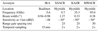
∗ Sensitivity for 2 s integration time and for nominal ARM radar settings.
2.3 Ikaalinen C-band weather radar
The Ikaalinen dual-polarization Doppler weather radar (IKA), used for cross-calibration analysis, belongs to the Finnish weather radar network (Saltikoff et al., 2010). It operates at C band and is located circa 64 km west of Hyytiälä. The antenna has a half-power beam width of 1∘. The radar performs volume scans, repeated every 5 min, and range height indicator (RHI) scans over the Hyytiälä site every 15 min.
The IKA data are quality-controlled and calibrated using a number of techniques. The engineering calibration, where different radar components are characterized, is performed during the radar installation and after major system modifications (Saltikoff et al., 2010). In addition to the engineering calibration, the radar receiver and antenna pointing are monitored using sun observations (Huuskonen and Holleman, 2010). The differential reflectivity calibration is monitored using a combination of vertically pointing scans and sun observations. During the summer months, the IKA radar absolute calibration was checked using the polarimetric self-consistency principle (Gorgucci et al., 1992; Gourley et al., 2009).
Given the continuous monitoring of the radar stability and regular calibration, we use the IKA observations as the calibration standard for the ARM radars. This approach allows us to cross-calibrate the ARM radars even in the presence of radome attenuation caused by, for example, large snow accumulation.
2.4 ARM cloud radar system calibration at X, Ka and W band
The ARM cloud radar systems operating at X, Ka and W band are integral part of the BAECC snowfall IOP. The antennas of the XSACR and KAZR are mounted on top of two containers located 17 m away from each other. The MWACR is mounted on the same container as KAZR. All the ARM radars make zenith-pointing observations. Looking at the radar technical properties in Table 1, the range gate spacing and the temporal sampling are comparable, but there is a difference in the beam width between XSACR and the other two systems. To reduce the beam mismatch and to facilitate the intercomparison with the ground-based sensors, all the radar data are averaged to 5 min. To derive consistent X-, Ka- and W-band Ze–S relations, the measured radar reflectivity factors were calibrated and corrected for attenuation. The absolute calibration of ARM cloud radars has been performed at the beginning and during the BAECC IOP using engineering calibration and external standard target procedure.

Figure 1Panel (a) shows radar profiles at C, X, Ka and W band for 15 February 2014 at 17:13 UTC where calibration is performed within the most stable height interval between 4 and 6 km. Panel (b) shows calibration error histograms related to the differences (Δ) between X- and C-band radars (dark red), Ka- and X-band radars (orange), and W and Ka radars (yellow).
We have also performed a cross-calibration in order to reduce biases between different radar systems. The cross-calibration method is based on the assumption that in the low reflectivity region at the cloud top the small crystals basically scatter in the Rayleigh regime (Hogan et al., 2000). We have compared the radar measurements in regions close to cloud top (height higher than 5 km) in non-precipitating ice clouds. The selected radar reflectivity profiles have reflectivity values of less than 0 dB. Furthermore, only cases where no lower clouds or precipitation were detected were used for calibration. The cross calibration was performed for all the cases before and after the snowfall events. Only events where the cross-calibration values did not change are used in this study. As mentioned in Sect. 2.3, the IKA radar observations are considered to be the reference for this analysis. The main reason for this selection is that the IKA radar is very stable and its performance is well monitored. Additionally, given its operating frequency, it does not suffer from attenuation during winter storms. Figure 1a shows the profile of 15 February 2014 at 17:13 UTC in which we performed the calibration between 4 and 6 km and in Fig. 1b the histograms of the three different calibration errors. The calibration error, measured as the standard deviation (SD) of the histograms in Fig. 1b, shows that the best result is for the error between Ka and W band and the worst is for C and X band, this being related mostly to the beam width. Looking at Table 1, it can be seen that the larger the beam width, greater the measured dispersion and vice versa.

Figure 2Relative frequency histograms of the sky-noise antenna temperature for the Ka- and W-band radars for all 10 days of the BAECC IOP campaign.
One of the reasons for differences in reflectivity measurements can also be attributed to the radome attenuation. For example, the flat shape of the KAZR radome increases the possibility of snow accumulation during a storm. Consequently, when the temperature rises above the melting point of ice, the melting snow could produce heavy attenuation that should be monitored. On the other hand, the conical shape of the MWACR radar limits the amount of accumulated snow, but because of the higher operating frequency it is more sensitive to the freezing rain/drizzle. To monitor the radome attenuation sky-noise analysis has been performed for the millimeter-wavelength radars, KAZR and MWACR. The sudden changes in the sky-noise temperature could have resulted from the increased surface temperature, which may indicate snow melting, and thus increased radome attenuation. The data in these cases are discarded. The stability analysis made with the sky noise is shown in Fig. 2 as a histogram of sky-noise power measured during 10 snowfall days of BAECC IOP. The SD is around 0.25 and 0.14 dBm, respectively, for KAZR and MWACR radar; according to these values, cases during the 10 snowfall events are excluded from the cross-calibration. This is shown in the Ka-band histogram in Fig. 2, where a secondary Gaussian-like peak is visible centered around −68.06 dBm.
During the BAECC IOP, radiosondes were launched four times a day. Using these observations as the input to the millimeter-wave propagation model (Liebe, 1985), the two-way gaseous path attenuation was computed for the dataset. This computation has been performed for all the dataset. For example, for 15 February 2014 at 17:24 UTC, the Ka-band two-way gas attenuation is 0.4334 dB. For the same time sample, the W-band two-way gas attenuation is 1.0206 dB. As expected, the attenuation for the W band is about twice as large as for Ka band. By taking into account the gaseous attenuation, the radar calibration offsets during the snowfall experiment were estimated as 2.9 dB for the XSACR, 3.9 dB for the KAZR and 4 dB for the MWACR. The results shown for the case study of 15 February 2014 have also been checked for the other snow events inside the dataset, confirming the consistency of the calibration analysis.
The focus of this study is to investigate the consistency of Ze–S relations at different frequencies, namely at X, Ka and W band. Given the current discussion on scattering properties of ice particles at millimeter wavelengths (Kneifel et al., 2018), the derived multi-frequency Ze–S relations are used to test the soft-spheroid model and compared with DDA scattering simulation.
3.1 Deriving Ze–S relations at X, Ka and W band
The equivalent reflectivity factor Ze, measured by the radar systems at different wavelengths, and the liquid-water-equivalent snowfall rate S, evaluated from PIP, are the two related variables. The S (in mm h−1) is derived from mass flux as
where m is the mass (in g), v is the velocity (in m s−1), N is the particle size distribution (PSD, in ) and ρw is the liquid water density (in g cm−3). In Eq. (1) all quantities are expressed in terms of the disk-equivalent diameter D=DDeq and derived from PIP measurements (von Lerber et al., 2017).
The radar data used in this study were collected in the vertical pointing mode. To match radar and in situ measurements, the radar data at the lowest meaningful altitude were used. Given the different radar specifications (see Table 1), the Fraunhofer far-field distance for the radars is different. This distance defines the near-field of the radars and is related to the radar antenna size. The beam width difference is related to the antenna diameter, which is respectively 1.82, 1.82 and 0.9 m for XSACR, KAZR and MWACR, so that the Fraunhofer distance (2D2∕λ) is approximately 214 m for XSACR, 773 m for KAZR and 514 m for MWACR. Taking into account the near-field influence, all radar data are selected at 400 m (Sekelsky, 2002).
Another important aspect is related to the different time acquisitions for the various instruments. In Table 1 we note that the temporal sampling of the radars is 2 s, whereas for the PIP instrument it is 1 min. To ensure similar sampling, we have decided to average data over 5 min. This results in PIP sampling volume of roughly 1 m3 for ice particles falling with a fall velocity of 1 m s−1. As mentioned in Sect. 2, the averaging is also useful to tackle the differences in radar beam widths.
The Ze–S is expressed in a power-law form, Ze=aSb, where Ze is in mm6 m−3 and S is in mm h−1 (Carlson and Marshall, 1972; Matrosov et al., 2008). In order to estimate the regression coefficients, we can choose nonlinear least squares in the variable linear space or linear least squares in the log–log variable space. We have adopted the latter approach by applying a linear regression as in Boucher and Wieler (1985). The applied log–log model is given by
where Ze can be either the time-averaged range-resolved co-polar radar measurement (disregarding the near-field effects) or the numerically simulated backscattering radar response.
3.2 Multi-frequency Ze–S relations using T-matrix scattering model
Single-scattering computations for spheroids are performed using Python implementation (Leinonen, 2014) of the TMM code (Mishchenko, 2000). The spheroidal particle model has been widely used for describing raindrops but also for approximating more complex particles such as snowflakes (Matrosov, 2007; Dungey and Bohren, 1993). In this study the spheroid model is initiated by using retrieved snowflake masses and maximum dimensions. This leaves the spheroid aspect ratio as a free parameter that adjusts volume, density and therefore the refractive index.
The aspect ratio is defined as , where as and bs are the horizontal and vertical dimensions of the spheroid (rs=1 spherical particle, rs≥ 1 prolate particle and rs≤ 1 oblate particle) (Dungey and Bohren, 1993). The snowflakes, due to aerodynamic forcing, typically fall with the major axis preferentially oriented horizontally (Magono and Nakamura, 1965; Matrosov, 2007). We have modeled the spheroids preferentially horizontally oriented with 10∘ SD of the canting angle distribution following Matrosov (2007) and Matrosov et al. (2008). It should be noted that while snowflakes in the nature may have wider orientation angle distributions, the goal of the particle models used for scattering computations is to provide a link between radar observation and cloud/precipitation properties such as snowfall intensity or ice water content. This goal does not necessary imply that all of the particle model properties coincide with properties of naturally occurring snowflakes. Our studies show that use of wider canting angle distributions results in worse agreement between measured and computed radar reflectivity values (Tyynelä et al., 2011).
To test whether the spheroidal model can produce consistent multi-frequency radar observations, the TMM computations are performed using different aspect ratios. If the computations with the same aspect ratio value can explain measured Ze–S relations at all the frequencies, then the spheroidal model can be considered adequate. If different aspect ratios are needed, then the model has failed. As stated above, the aspect ratio defines particle density as
in which the mass m is defined as in von Lerber et al. (2017) and DVeq is the volume equivalent diameter defined from Dmax, the maximum diameter obtained by PIP (von Lerber et al., 2017), as DVeq = . The presence of the aspect ratio inside the density reflects its influence on the complex refractive index of snow mS that is defined through the Maxwell Garnett EMA.
The Γ-size distribution (in ) is assumed to model the PSD:
where Nw,Veq is the intercept parameter (in ), f(μVeq) and μVeq parameters are dimensionless, ΛVeq is the slope of the distribution in 1 mm−1 and D0,Veq is the median volume diameter in mm. This Γ-size distribution can be expressed starting from the moments of the snowflake distributions measured by PIP, as in Bringi and Chandrasekar (2001), taking into account the variable changing from Dmax to DVeq as follows:
with
In the computations we have used the Γ-modeled size distribution, with the maximum dimension of 2.5 D0,veq.
3.3 Multi-frequency Ze–S relations using DDA scattering model
The DDA model is used to characterize the single-scattering properties of snowflakes when described with complex and more realistic shape models. Because of computational reasons, here DDA is not used to compute the scattering properties of the observed snowflakes, but rather the pre-calculated lookup tables (LUTs) are utilized for realistically shaped particles. Leinonen and Szyrmer (2015) have published an extensive LUT of backscattering properties for realistically modeled unrimed and rimed snow particles. The shape model is obtained by accurately simulating the microphysical processes that lead to snowflake growth. In particular, the snowflake formation is simulated by aggregation of pristine dendrites and subsequent or simultaneous riming of those aggregates using multiple values of equivalent LWP which in turn determine the degree of riming. The simulation of the riming process provides the scattering database to span through a large range of particle masses and sizes allowing to use those microphysical features to constrain the ice particle scattering properties. Moisseev et al. (2017) have shown that during BAECC experiment snow particles were moderately to heavily rimed; therefore the selection of the database that includes rimed particles appears to be justified. The scattering properties of the simulated particles are in fact picked from the LUT by finding the entries that most closely match the retrieved particle size and mass in von Lerber et al. (2017).
According to the PSD bin sizes of the PIP, the LUT is filtered to find entries which falls within each bin category. Then, using the retrieved m(D) relation determined in von Lerber et al. (2017) the LUT entries are sorted with respect to the difference between their mass, and the expected particle mass is computed using the retrieved m(D) relation. An arbitrary number of 10 entries that most closely match the retrieved m(D) relation are selected and their scattering properties are averaged in order to define the representative backscattering cross section of that particular size range. Larger number of particles can be picked from the LUT in order to represent a larger variability of particle mass, but the effects of including heavier and lighter particles tend to cancel out in the averaging and do not produce notable differences in the final integrated reflectivity value.
It is worth noting that the particles of Leinonen and Szyrmer (2015) are partially horizontally aligned where orientation of their shortest principal axis is, being normally distributed, with the SD of 40∘.
The results are shown for four snowfall events during BAECC to investigate the consistency of Ze–S relations at X, Ka and W bands using surface observations. Indeed, 10 snowfall cases are available from the BAECC IOP, but only for the selected four events can the millimeter-wave radars (Ka and W bands) be considered well calibrated, in the other cases effects of the radome attenuation cannot be fully removed. K-means cluster analyses were applied to identify three riming subgroups. The uncertainties of the Ze–S parametric relations at different frequencies are also investigated using TMM and DDA numerical results. The TMM and DDA results can provide some microphysical insights into the considered snowfall events.
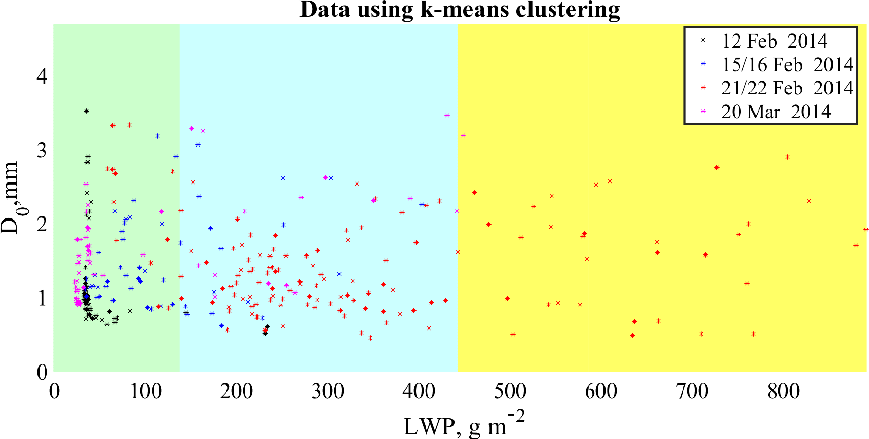
Figure 3Plot of median diameter D0 with respect to LWP for the three cluster regions, LR, MR and HR, (green, cyan, yellow) obtained on four snowfall days of BAECC IOP campaign. Black, blue, red and magenta points respectively represent the data for 12, 15/16, 21/22 February and 20 March 2014. The k-means clustering highlights the weak dependence of the classes from D0.
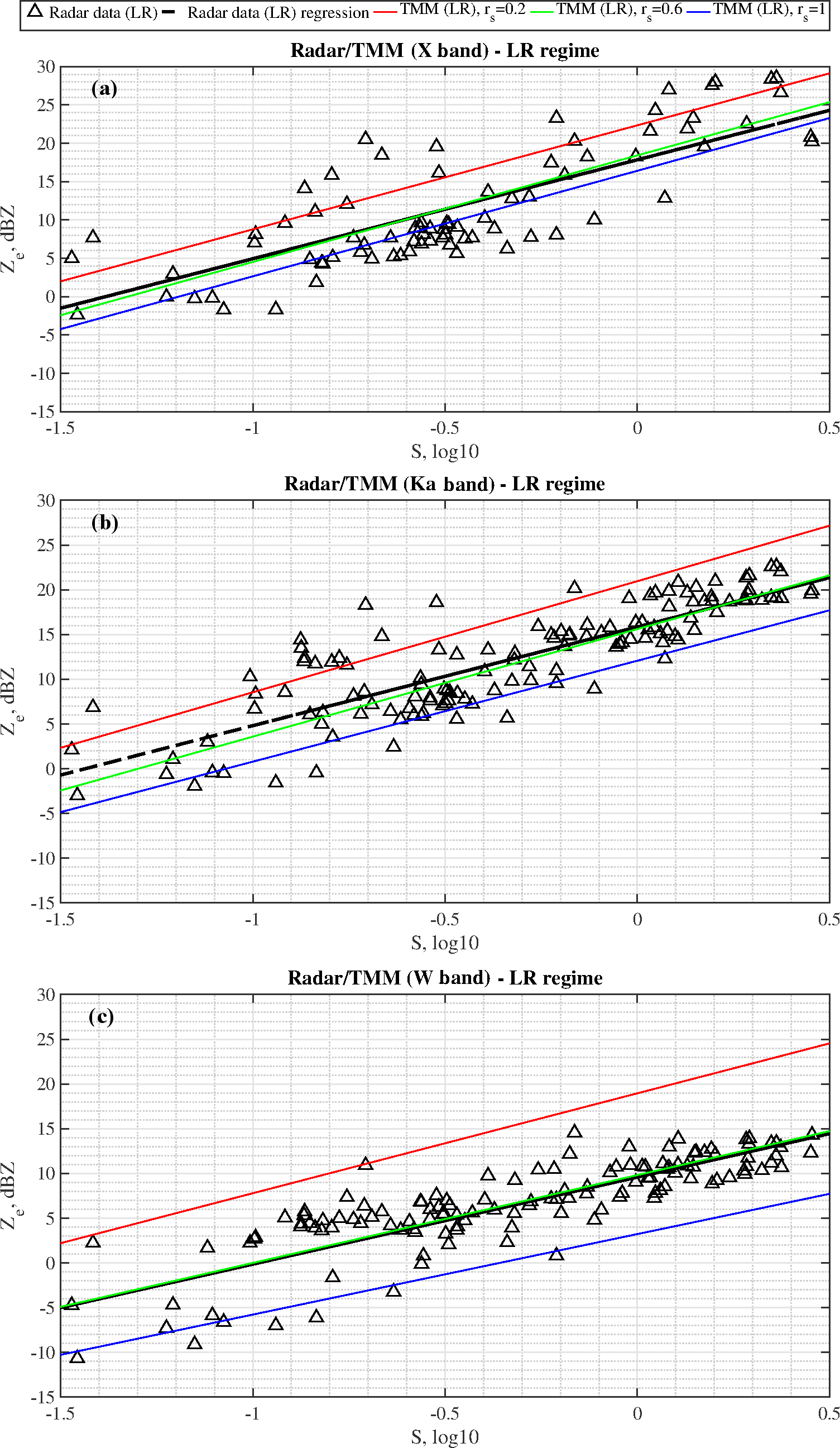
Figure 4Case for lightly rimed (LR) snowfall: (a) X-, (b) Ka- and (c) W-band results. Scatter plot of the equivalent radar reflectivity, measured by ARM radars (black triangles), with respect to the snow rates, S, measured by PIP. The black line represents the Ze–S empirical least-squares relationship as listed in Table 2. Ze–S parametric relations, derived from TMM-based simulations, are also shown for different aspect ratios (0.2, 0.6, 1) using red, green and blue lines as listed in Table 4.

Figure 5Same as Fig. 4 but for moderately rimed (MR) snowfall cases. Scatterplot is now represented by black circles.
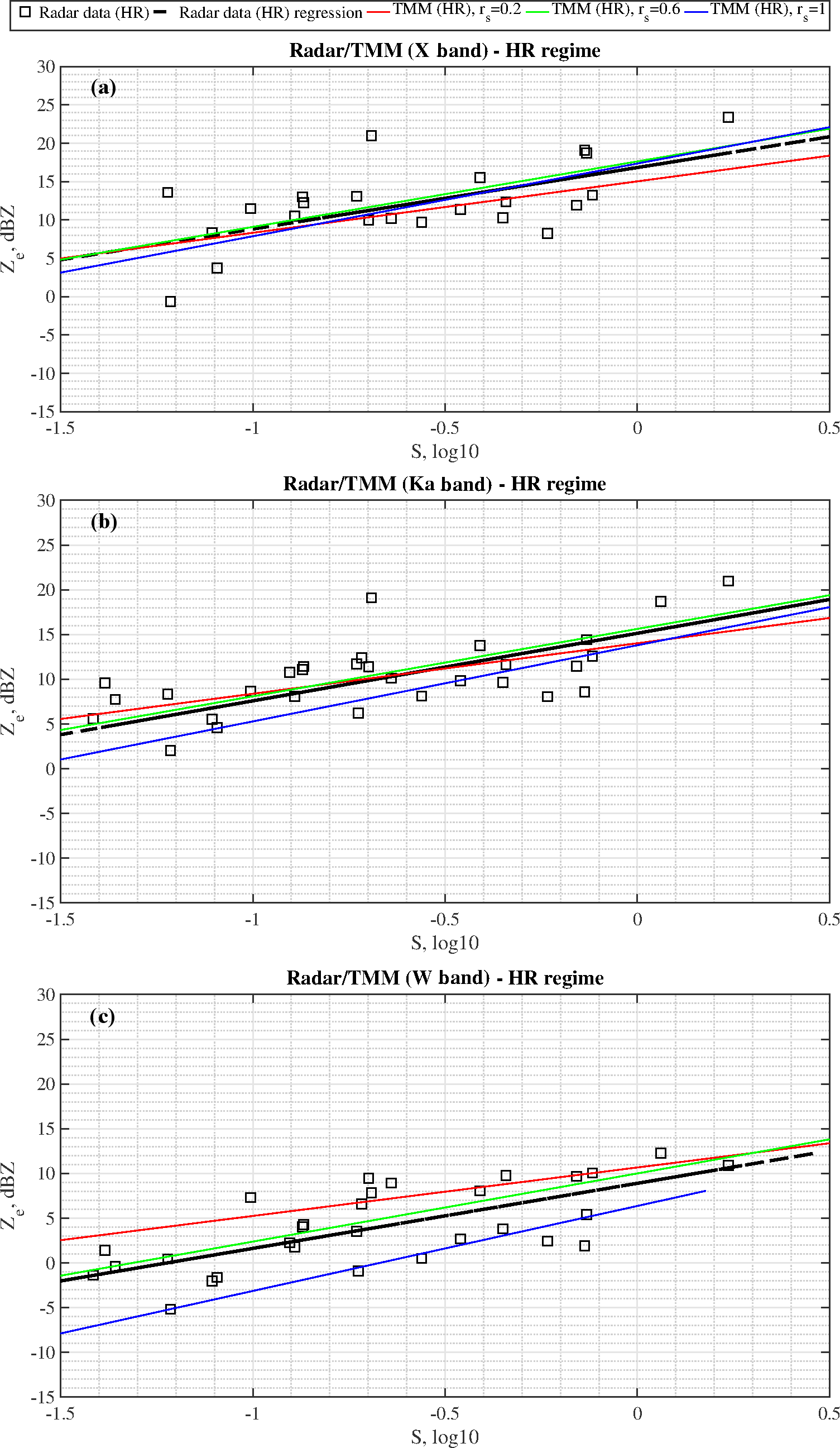
Figure 6Same as Fig. 4 but for heavily rimed (HR) snowfall cases. Scatterplot is now represented by black squares.
4.1 Analysis of X, Ka and W bands Ze–S empirical relations
The dataset was divided into three riming classes – lightly, moderately and heavily rimed (LR, MR and HR) snow – following the same logic used presenting the m(D) relations in von Lerber et al. (2017). Case studies were divided into classes using LWP values for the direct correspondence to the degrees of riming. Since the ice particle mass growth rate due to riming is proportional to LWP along the particle fall trajectory, the LWP can be seen as a proxy for riming (e.g. Moisseev et al., 2017). Given the growth rate, the riming degree of snowfall may also be influenced by the average particle size, such as D0. To take all of this into account, the presented four snowfall events were classified into three subgroups using a k-means cluster analysis trained by LWP and D0. The results are presented in Fig. 3 where the three clusters are identified in the LWP-D0 space. It is worth noting that riming is strongly related to LWP but almost not dependent on the estimated size D0 of snow particles. In summary, we have analyzed four events for Ka and W bands and three cases (excepted 20 March 2014) for X band. For the Ka and W band radar observations we have 282 data samples, which correspond to 1410 measurement minutes, of which 50.35 % are LR, 37.23 % MR and 12.42 % HR. For X band we have 174 data samples, 870 measurement minutes, divided into 49.42 % of LR, 35.06 % of MR and 15.52 % of HR. In Figs. 4–6 the derived Ze–S relations for all radar frequencies and riming classes are presented.
Table 2Empirical Ze–S for the four snow cases divided into LR, MR and HR snowfall regimes as shown in Figs. 4–6. Ze–S at X, Ka and W band derived from ARM radar and PIP video disdrometer using a least-squares regressive analysis in the log–log space for each riming regime. The root-mean-square error (RMSE) is also shown in addition to the normalized RMSE (NRMSE) for the value range (defined as the maximum value minus the minimum value) of the measured data. The variability of coefficients, a and b, is shown in Fig. 7. Coefficients are related to the Ze–S reference model in power-law form, i.e., Ze=aSb, where Ze is expressed in mm6 m−3 and S is in mm h−1.
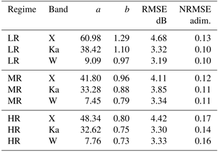
BAECC cases of snowfall events with the a and b coefficients estimated in a 5 min time window.
Table 3The prefactors and exponents of the Ze–S relation in the literature for X, Ka and W band.
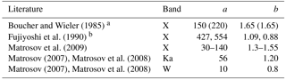
a Boucher and Wieler (1985) provided a mean X-band relation between snowfall depth SS and
equivalent radar reflectivity as Ze = . This relation is expressed in Table for the snow-to-liquid ratio of 8:1 (10:1).
b Fujiyoshi et al. (1990) presented a best-fit power-law
relationship using 1 and 30 min respectively of averaged S and
Ze.
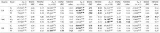
Table 4Ze–S (with Ze in mm6 m−3, S in mm h−1) relationships for all three riming classes, derived from TMM-based numerical simulations of Ze and PIP-derived S and using the oblate-particle aspect ratio as a tuning parameter between 0.2 and 1. The best Ze–S relation is highlighted in bold and corresponds to the power-law minimizing both RMSE and NRMSE.
The LR snowfall samples are plotted in Fig. 4, showing the retrieved liquid-water-equivalent snowfall rate S from PIP (see in Eq. 1) with respect to the measured equivalent reflectivity factor Ze from the ARM radars. A representation with Ze in dBZ and S in base-10 logarithm has been chosen to adhere to the log–log model in Eq. (2). The parameters of the three Ze–S relations are given in the Table 2. The accuracy of Ze–S relations has been evaluated using the root-mean-square error (RMSE) in dB (where the error is defined as the difference between observed Ze and estimated from PIP, using the regression coefficients). The normalized RMSE (NRMSE), i.e., RMSE values normalized by the observed reflectivity range, is also presented in the table. The NRMSE in percentages of the regressions shown in Fig. 4 is about 13 and 10 % for X and Ka/W band, respectively. Both prefactors and exponents of the Ze–S relations tend to decrease with the radar frequency increase similar to what is presented in Matrosov (2007) and Matrosov et al. (2008). The regression coefficients are very close to those of Matrosov (2007) and Matrosov et al. (2008) and are rather different from those of Boucher and Wieler (1985) and Fujiyoshi et al. (1990). The literature values of the Ze–S relations are summarized in Table 3.
Similar to the light riming class, the MR snowfall Ze–S observations are shown in Fig. 5. The prefactor, a, and exponent, b, are slightly different with respect to the LR snowfall class; they decrease with the frequency but they have lower values, especially for X band. The trend of the a coefficient can also be considered in line with Matrosov (2007) and Matrosov et al. (2008), while the b coefficient is close to Matrosov (2007) and Matrosov et al. (2008) only for W band.
The last result is for HR snowfall, presented in Fig. 6. The values of the a and b coefficients are lower than those of the previous two riming regimes and than those of Matrosov (2007) and Matrosov et al. (2008), having a worse NRMSE accuracy of about 17 % (X band), 14 % (Ka band) and 16 % (W band).
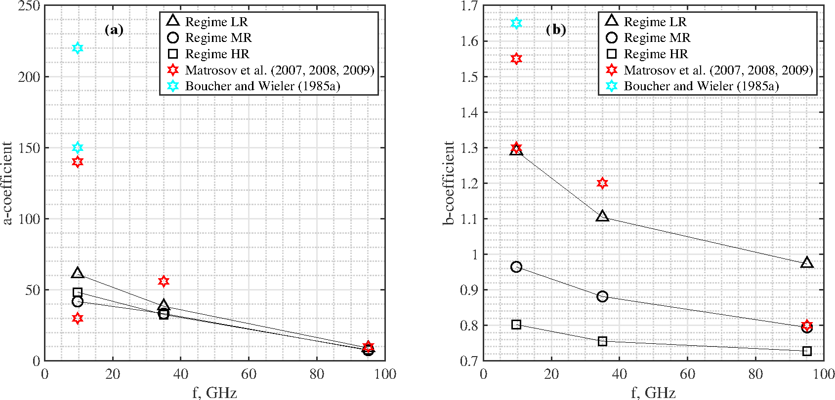
Figure 7Frequency trend for the a (a) and b (b) regression coefficients, estimated in Table 2 using the power-law form Ze=aSb for the four studied snowfall cases divided into LR, MR and HR.
Using data of the studied snowfall cases, the frequency behavior of the a and b power-law coefficients in Table 2 may be useful to suggest a general trend of the Ze–S relation, even though only three frequency at X, Ka and W band are available. Figure 7 shows the spectral variation of the a and b coefficients, splitting the results between lightly rimed snowfall (black triangles), moderately rimed (black circles) and heavily rimed snowfall classes (black squares). The spline interpolation has been introduced for the three riming classes to outline a possible trend for these two coefficients. Considering all the limitations of the presented analysis it is still worth noting that (i) the monotonic decrease in the a coefficient with the frequency has been noted for all the three classes in Fig. 7a (the slope is higher for the LR with respect to the MR and HR), and (ii) the different spectral trend of the b coefficient in Fig. 7b decreases with the frequency, but it could be also used to separate the three regimes.
While analyzing the presented Ze–S relation trends, we should understand that these relations depend on PSD parameters, such as Nw, m(D) and corresponding single-scattering ice particle properties. The difference between Ze–S obtained for different radar frequency bands arises from the changes in the snowflake scattering properties. In the Rayleigh regime, the dependence of radar cross section (RCS), on D, is given by m(D)2. For higher frequencies the exponent of RCS(D) relation will become smaller, and therefore the exponent of Ze–S relation should decrease as well. However, the relations derived for different snowfall riming regimes are influenced not only by changes in m(D) but also by changes in PSD. Furthermore, here not only changes in average values of, for example, Nw are important but also PSD parameter variations during the recorded events (von Lerber et al., 2017). Therefore, some of the changes in the a and b coefficients between the riming classes are probably caused by the PSD values and variations.
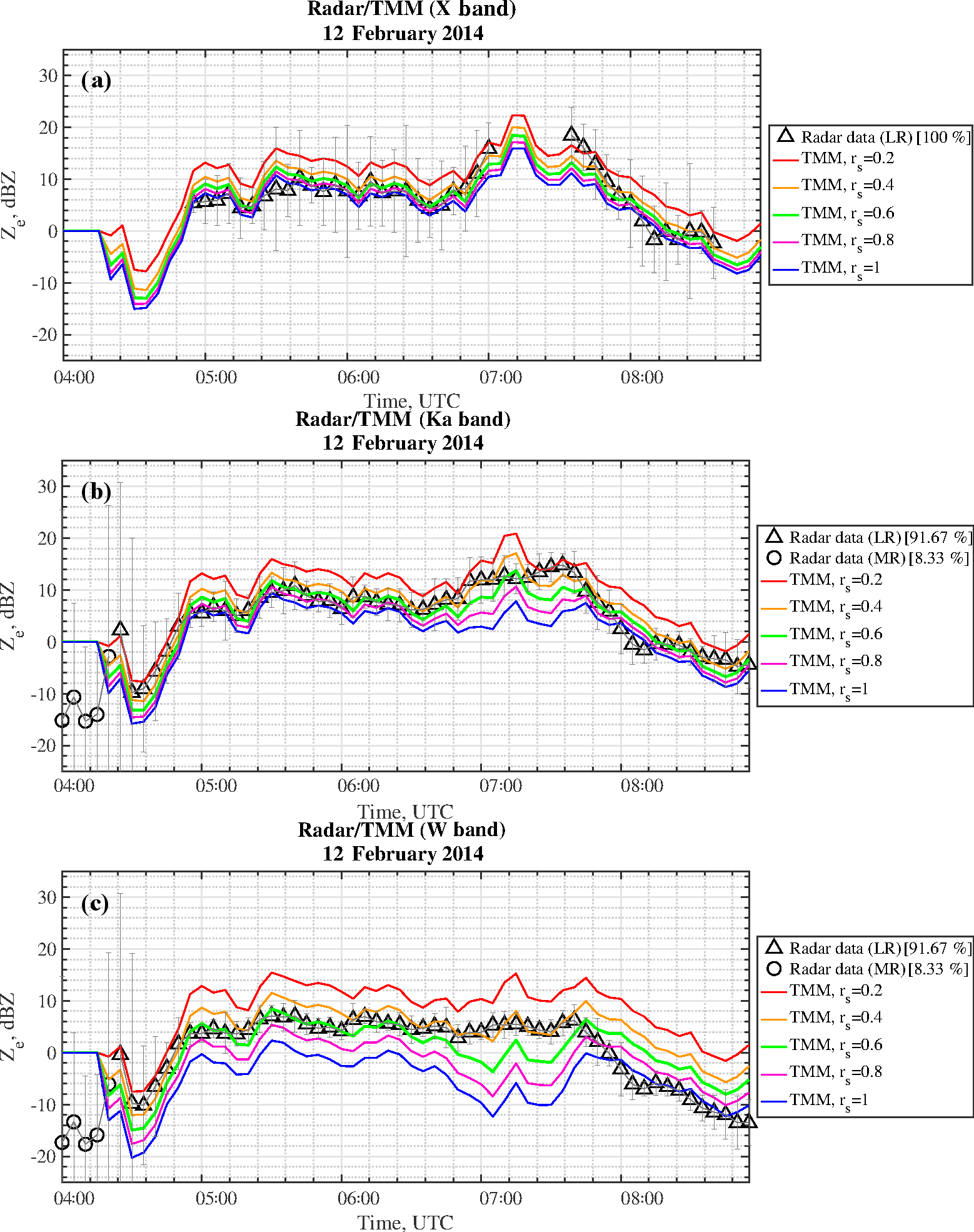
Figure 8Radar and TMM computations from 12 February 2014 between 04:00 and 08:50 UTC for (a) X band, (b) Ka band and (c) W band. Radar reflectivities (LR and MR snowfall in black triangles and circles, respectively) from XSACR, KAZR and MWACR are corrected for sky-noise, calibration offsets and attenuations (as better explained in Sect. 2.4). The error bars are used to represent the variation (min–max difference) of radar data within a 5 min window with respect to their averaged value (black triangles and circles). TMM-based computations (red, orange, green, magenta and blue lines for rs=0.2, rs=0.4, rs=0.6, rs=0.8 and rs=1, respectively) are derived from PIP data.
4.2 Explaining Ze–S relations with scattering simulations
Time series of multi-frequency radar measurements can provide a further insight into the analysis of snowfall regime and the capability to simulate its behavior. Figure 8 shows the equivalent reflectivity factor Ze as a function of time for the snow case study of the predominantly LR 12 February 2014 case (100 % for X band, 91.67 % for Ka/W band). The black triangles and circles correspond to ARM-radar mean Ze, whereas the bars are related to the variation between their minimum and maximum values within the same averaging time interval of 5 min. A total of 8.33 % of the measurements (black circles in Fig. 8b and c) at the beginning of the event correspond to the MR snow data (0 % for X band, 8.33 % for Ka/W band) and they are disregarded since the variation index (defined as the ratio between minimum–maximum variability interval and its mean value) is considered to be too high. The different colored lines refer to Ze, simulated using TMM from PIP data with a variable aspect ratio rs between 0.2 and 1 with a step of 0.2. The smaller value rs = 0.2 (red line) indicate very oblate particles, whereas rs = 1.0 (blue line) correspond to spherical snowflakes. By comparing ARM measurements and TMM simulations, the optimal aspect ratio value seems to decrease when increasing the frequency: X-band data are better represented by TMM-derived spherical particles (rs=1), whereas Ka- and W-band results are in agreement with an aspect ratio of 0.6. After 07:00 UTC within the heavy precipitation period, no data are available for X-band radar in this case study, but the optimal aspect ratio tend to change to a value around of rs=0.4 for the millimeter-wave radars (Ka and W band). This frequency dependence of the aspect ratio indicates that the soft-spheroid model is not consistent across the frequencies, for this snow event. This finding is in line with Leinonen et al. (2012) and Kneifel et al. (2015), who showed that for low-density aggregates the soft-spheroid model may not be adequate.
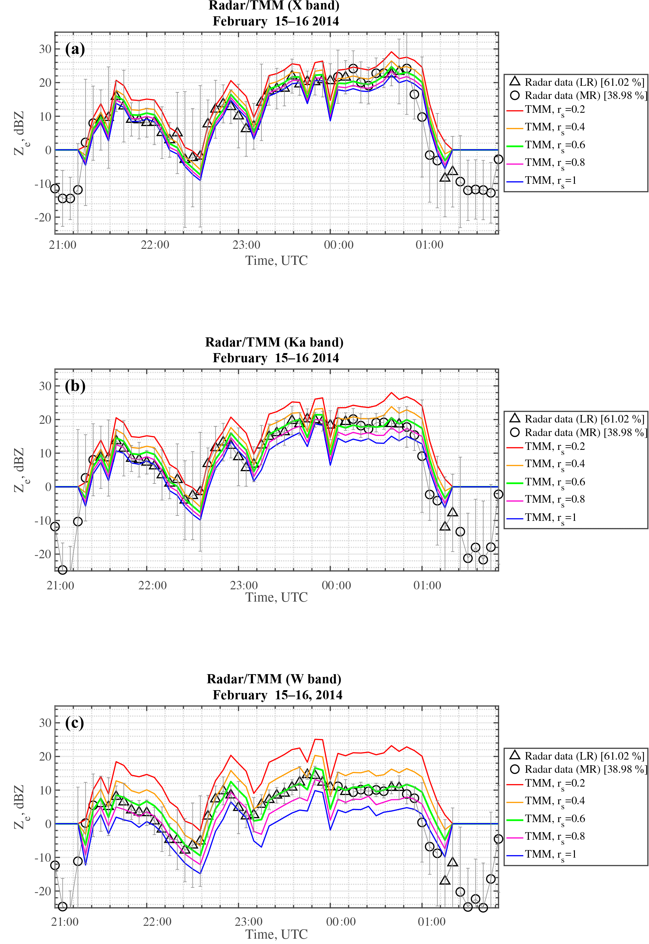
Figure 9Same as Fig. 8, but for 15/16 February 2014, 21:00–01:48 UTC (LR and MR snowfall in black triangles and circles, respectively).
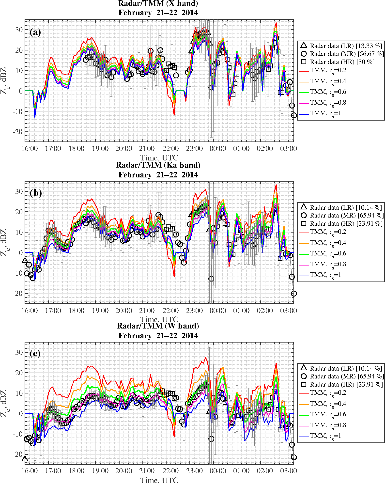
Figure 10Same as Fig. 8, but for 21/22 February 2014, 16:00–03:24 UTC (LR, MR and HR snowfall in black triangles, circles and squares, respectively).

Figure 11Same as Fig. 8, but for 20 March 2014, 16:00–20:48 UTC (LR, MR and HR snowfall in black triangles, circles and squares, respectively). The X-band radar data are not available for this time window.
Figure 9 again shows Ze as a function of time for the mixed LR–MR 15–16 February 2014 snowfall case (61.02 % for LR and 38.98 % for MR). We can distinguish two main intervals: before the heavy precipitation around 22:10 UTC, as for the previous case, the optimal aspect ratio decreases when increasing the radar frequency, whereas during the heavy precipitation interval (from 22:50 UTC on) the optimal aspect ratio seems to be around 0.6 independent of the frequency that corresponds to the LR time period. Figure 10 shows the time behavior for 21–22 February 2014, a snow case with all three regimes present (X band: 13.33 % for LR, 56.67 % for MR and 30 % for HR; Ka/W band: 10.14 % for LR, 65.94 % for MR and 23.91 % for HR). Until 22:00 UTC, in the presence of MR snow, the optimal aspect ratios seem to be around 1, 0.8 and 0.8 at X, Ka and W band, respectively, whereas during the heavy precipitation period (23:00–00:00 UTC), in the presence of LR snow, it is constant around rs=0.6 irrespective of the frequency. These considerations are also valid for 20 March 2014 in Fig. 11, in which the optimal aspect ratio is about rs=0.6 for the millimeter-wave radars (Ka and W band) and in fact it was a predominantly LR case (72.41 % for LR, 24.14 % for MR and 3.45 % for HR). For this case X-band data are not available and thus they are not shown in the figure.
As a general comment on Figs. 8–11, we note that measured data fall within the computed range of uncertainty. The incremental difference in terms of Ze due to an increase of 0.2 in the particle aspect ratio is about 1.7 dBZ at X band, 2.5 dBZ at Ka band and 6 dBZ at W band. The difference between the value for rs=0.2 and rs=1 is on average 5.5 dBZ for X band, 7 dBZ for Ka band and 12 dBZ for W band. By increasing the frequency from X to W band, the radar reflectivity seems to be, in general, more sensitive to the non-spherical shape of the snowflakes, with rs decreasing from 1 to 0.6.
To investigate how the soft-spheroid model performs in terms of reproducing the observed Ze–S relations, the TMM computed reflectivity factors were used to derive multi-frequency Ze–S relations. The relations were computed using different values of the soft-spheroid model aspect ratio. The derived relations are summarized in Table 2 and shown in Figs. 4, 5, and 6. Similar to the analysis of the Ze time series, presented above, we may conclude that to reproduce the observed Ze–S relations at different frequencies, different spheroid aspect ratios may need to be used. This effect is clearest for the LR class (see Fig. 4), where for X band the best fitting aspect ratio is 1 and for W band it is closer to 0.6. For heavier rimed particles this difference becomes less pronounced.
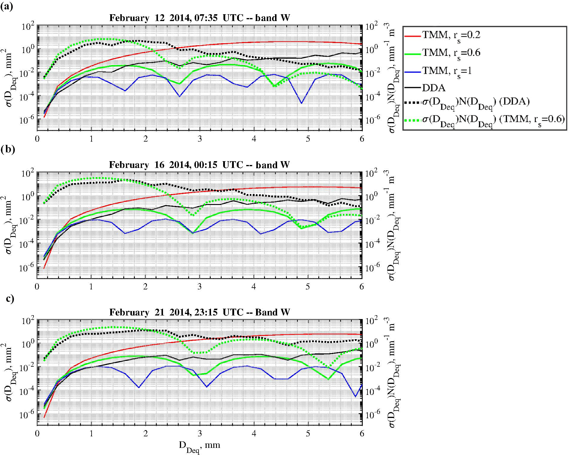
Figure 12Horizontally polarized cross section σ, expressed as a function of the diameter disk-equivalent DDeq at W band by comparing DDA computations (black line) and TMM computations (red, green and blue lines, matching rs=0.2, rs=0.6 and rs=1). The product between σ and PIP-derived snowflake size distribution N shows the main contribution of particle size in terms of diameter disk-equivalent for DDA computations (dotted black line) and TMM computations (rs=0.6, dotted green line).
It should be noted that the observed differences between observed Ze and ones computed using TMM are not as large as was previously expected. To investigate why this is the case, single-scattering properties computed using DDA (Leinonen and Szyrmer, 2015) were compared to the TMM results for the three cases shown in Fig. 12. The computations are performed for the W band. TMM simulations are given by red, green and blue lines referring to different aspect ratios (rs=0.2, 0.6, 1, respectively), whereas DDA results are given by the black line. The dotted line shows the product between the snowflake PSD and the RCS computed using TMM with aspect ratio of 0.6 (green dotted line) and the DDA (black dotted line). This figure shows that TMM computations using lower aspect ratios agree better with DDA. Furthermore, it indicates that there is a compensating effect, where TMM overestimates RCS for smaller snowflakes and underestimates it for larger particles. This may explain smaller differences between the DDA and TMM calculations.
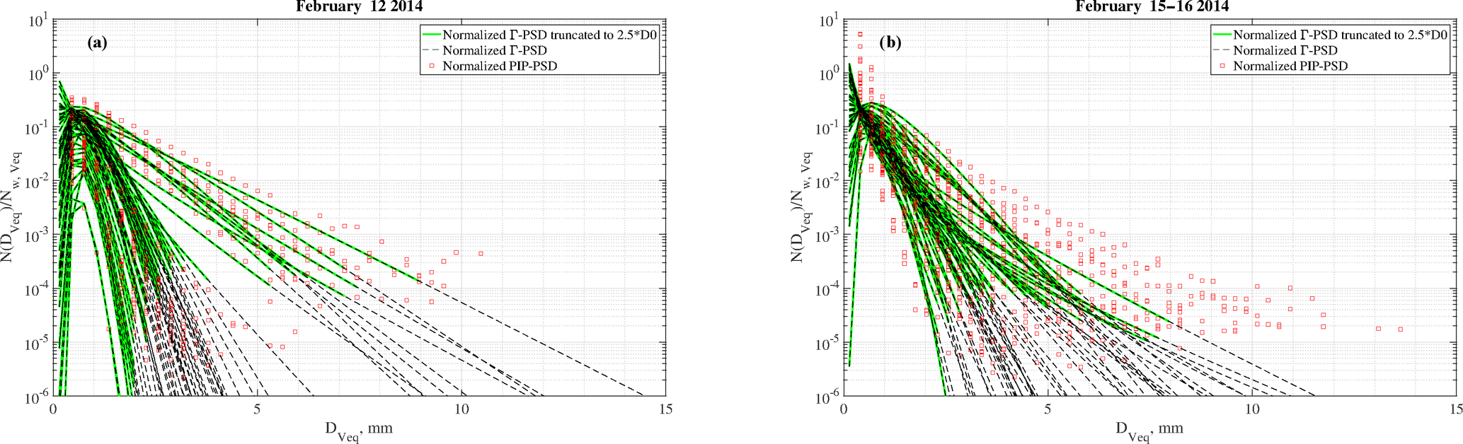
Figure 13Panel (a) shows PSD for snowfall case of 12 February 2014 and (b) shows PSD for snowfall case of 15/16 February 2014. Red circles are representative of the normalized PSD measured by PIP, the dashed black line represents the normalized estimated Γ-PSD in Eq. (4) and the green line is the last one truncated at the maximum value of 2.5 multiplied by the median diameter D0.
This compensation effect depends on the integration limits used to compute the Ze. In this study we have integrated from 0 to 2.5 D0. To check whether this integration limit is valid, in Fig. 13 measured and fitted PSDs are shown. As can be seen, the assumed upper integration limit appears to be valid.
The multi-frequency Ze–S relationships at X, Ka and W bands have been investigated in this work using a dataset of zenith-pointing radar data and in situ measurements acquired during the BAECC campaign.
From a data analysis point of view, adopting as a reference a power-law relation, regression coefficients have been extracted for characterizing Ze–S at the considered frequency bands. These coefficients are in line with those provided in the literature and also confirm the applicability of a power-law empirical model to the millimeter-wave radars for snowfall estimation in different riming regimes. The latter can be schematically refer to as lightly, moderately and heavily rimed snowfall.
For validation and intercomparison, numerical simulations have been also carried out using the soft-spheroid model and TMM, coupled with microphysical PSD from an in situ video disdrometer and a retrieved mass-dimensional relation and using the particle aspect ratio as a tuning parameter. Uncertainty in each derived Ze–S relationship has been provided and ranked with respect to the available radar measurements of BAECC IOP. The latter show that there are specific spheroid aspect ratios for the three identified snowfall regimes. TMM numerical results have been also compared with DDA scattering simulation in order to better understand the role of the aspect ratio.
Uncertainty evaluation has been attached to each empirical and modeled power-law relationship at X, Ka and W band for each case study and for the three snowfall regimes. This set of regression coefficients may be used in the future for selecting optimal Ze–S algorithms in different geographical regions and to assess the dependence on the snowfall type. In this respect, the results of this work can represent a first step towards the design of snowfall retrieval algorithm derived from ground-based measurements and the setup of simplified scattering simulations for centimeter and millimeter wavelengths.
The ARM data used in this study are available from Atmospheric Radiation Measurement (ARM) Climate Research Facility (ARM Climate Research Facility, 1990, 1993, 2006, 2010, 2011). PIP data are available from https://github.com/dmoisseev/Snow-Retrievals-2014-2015 (last access: 10 January 2017).
The authors declare that they have no conflict of interest.
Marta Tecla Falconi was partly supported by the Center of Excellence CETEMPS, L'Aquila (Italy). The activity of Davide Ori was funded by the German
Research Foundation (DFG) as part of the Emmy Noether Group OPTIMIce under
grant KN 1112/2-1. Annakaisa von Lerber was supported by Horizon 2020 grant agreement no. 699221 (PNOWWA) and
no. 700099 (ANYWHERE). The research of Dmitri Moisseev was supported by the Academy of Finland (grant 305175) and the Academy
of Finland Finnish Centre of Excellence program (grant 3073314). Dmitri Moisseev also acknowledges the funding received
from
ERA-PLANET, trans-national project iCUPE (grant agreement no. 689443), funded under the EU Horizon 2020 Framework
Programme.
Edited by: Gianfranco Vulpiani
Reviewed by: five anonymous referees
Atmospheric Radiation Measurement (ARM) Climate Research Facility: KAZR Corrected Data (KAZRCORGE). 2014-02-12 to 2014-03-20, updated hourly, ARM Mobile Facility (TMP) U. of Helsinki Research Station (SMEAR II), Hyytiala, Finland; AMF2 (M1), compiled by: Matthews, A., Isom, B., Nelson, D., Lindenmaier, I., Hardin, J., Johnson, K., Bharadwaj, N., Giangrande, S., and Toto, T., Atmospheric Radiation Measurement (ARM) Climate Research Facility Data Archive: Oak Ridge, Tennessee, USA, https://doi.org/10.5439/1350632 (last access: 10 January 2017), 1990. a
Atmospheric Radiation Measurement (ARM) Climate Research Facility: MWR Retrievals (MWRRET1LILJCLOU). 2014-02-12 to 2014-03-20, updated hourly, ARM Mobile Facility (TMP) U. of Helsinki Research Station (SMEAR II), Hyytiala, Finland; AMF2 (M1), compiled by: Sivaraman, C., Gaustad, K., Riihimaki, L., Cadeddu, M., Shippert, T., and Ghate, V., Atmospheric Radiation Measurement (ARM) Climate Research Facility Data Archive: Oak Ridge, Tennessee, USA, https://doi.org/10.5439/1027369 (last access: 10 January 2017), 1993. a
Atmospheric Radiation Measurement (ARM) Climate Research Facility: MWACR Ship Motion Correction (MWACRSHIPCOR). 2014-02-12 to 2014-03-20, updated hourly, ARM Mobile Facility (TMP) U. of Helsinki Research Station (SMEAR II), Hyytiala, Finland; AMF2 (M1), compiled by: Matthews, A., Isom, B., Nelson, D., Lindenmaier, I., Hardin, J., Johnson, K., and Bharadwaj, N., Atmospheric Radiation Measurement (ARM) Climate Research Facility Data Archive: Oak Ridge, Tennessee, USA, https://doi.org/10.5439/1350621 (last access: 10 January 2017), 2006. a
Atmospheric Radiation Measurement (ARM) Climate Research Facility: Ka-Band Scanning ARM Cloud Radar (KASACRCRRASTER). 2014-02-12 to 2014-03-20, updated hourly, ARM Mobile Facility (TMP) U. of Helsinki Research Station (SMEAR II), Hyytiala, Finland; AMF2 (M1), compiled by: Matthews, A., Isom, B., Nelson, D., Lindenmaier, I., Hardin, J., Johnson, K., Lamer, K., Bharadwaj, N., Kollias, P., Giangrande, S., and Toto, T., Atmospheric Radiation Measurement (ARM) Climate Research Facility Data Archive: Oak Ridge, Tennessee, USA, https://doi.org/10.5439/1095596 (last access: 10 January 2017), 2010. a
Atmospheric Radiation Measurement (ARM) Climate Research Facility: X-Band Scanning ARM Cloud Radar (XSACRRHI). 2014-02-12 to 2014-03-20, updated hourly, ARM Mobile Facility (TMP) U. of Helsinki Research Station (SMEAR II), Hyytiala, Finland; AMF2 (M1), compiled by: Matthews, A., Isom, B., Nelson, D., Lindenmaier, I., Hardin, J., Johnson, K., and Bharadwaj, N., Atmospheric Radiation Measurement (ARM) Climate Research Facility Data Archive: Oak Ridge, Tennessee, USA, https://doi.org/10.5439/1150299 (last access: 10 January 2017), 2011. a
Böhm, H.: A general equation for the terminal fall speed of solid hydrometeors, J. Atmos. Sci., 46, 2419–2427, https://doi.org/10.1175/1520-0469(1989)046<2419:AGEFTT>2.0.CO;2, 1989. a, b
Botta, G., Aydin, K., and Verlinde, J.: Modeling of microwave scattering from cloud ice crystal aggregates and melting aggregates: a new approach, IEEE Geosci. Remote S., 7, 572–576, https://doi.org/10.1109/LGRS.2010.2041633, 2010. a
Boucher, R. J. and Wieler, J. G.: Radar determination of snowfall rate and accumulation, J. Clim. Appl. Meteorol., 24, 68–73, https://doi.org/10.1175/1520-0450(1985)024<0068:RDOSRA>2.0.CO;2, 1985. a, b, c, d, e
Bringi, V. and Chandrasekar, V.: Polarimetric Doppler Weather Radar: Principles and Applications, Cambridge University Press, Cambridge, UK, https://doi.org/10.1017/CBO9780511541094, 2001. a
Cadeddu, M.: Microwave radiometer (MWRLOS), ARM Mobile Facility TMP, University of Helsinki research station SMEAR II, Hyytiälä, Finland, Atmospheric Radiation Measurement (ARM) Climate Research Facility Data Archive, Oak Ridge, TN, https://doi.org/10.5439/1046211 (last access: 17 March 2016), 2014. a
Carlson, P. E. and Marshall, J. S.: Measurement of snowfall by radar, J. Appl. Meteorol., 11, 494–500, https://doi.org/10.1175/1520-0450(1972)011<0494:MOSBR>2.0.CO;2, 1972. a, b
Dungey, C. and Bohren, C.: Backscattering by nonspherical hydrometeors as calculated by the coupled-dipole method: an application in radar meteorology, J. Atmos. Ocean. Tech., 10, 526–532, https://doi.org/10.1175/1520-0426(1993)010<0526:BBNHAC>2.0.CO;2, 1993. a, b
Fujiyoshi, Y., Endoh, T., Yamada, T., Tsuboki, K., Tachibana, Y., and Wakahama, G.: Determination of a Z–R relationship for snowfall using a radar and high sensitivity snow gauges, J. Appl. Meteorol., 29, 147–152, https://doi.org/10.1175/1520-0450(1990)029<0147:DOARFS>2.0.CO;2, 1990. a, b, c, d
Goodison, B., Louie, P., and Yang, D.: WMO Solid Precipitation Measurement Intercomparison Final Report, Tech. Rep. WMO/TD No. 872, IOM No. 67, World Meteorological Organization (WMO), Geneva, Switzerland, 1998. a
Gorgucci, E., Scarchilli, G., and Chandrasekar, V.: Calibration of radars using polarimetric techniques, IEEE T. Geosci. Remote, 30, 853–858, 1992. a
Gourley, J., Illingworth, A., and Tabary, P.: Absolute calibration of radar reflectivity using redundancy of the polarization observations and implied constraints on drop shapes, J. Atmos. Ocean. Tech., 26, 689–703, 2009. a
Gunn, K. L. S. and Marshall, J. S.: The distribution with size of aggregate snowflakes, J. Meteorol., 15, 452–461, https://doi.org/10.1175/1520-0469(1958)015<0452:TDWSOA>2.0.CO;2, 1958. a
Hogan, R. J., Illingworth, A. J., and Sauvageot, H.: Measuring crystal size in cirrus using 35- and 94-GHz radars, J. Atmos. Ocean. Tech., 17, 27–37, https://doi.org/10.1175/1520-0426(2000)017<0027:MCSICU>2.0.CO;2, 2000. a
Huuskonen, A. and Holleman, I.: Determining weather radar antenna pointing using signals detected from the sun at low antenna elevations, J. Atmos. Ocean. Tech., 24, 476–483, https://doi.org/10.1175/JTECH1978.1, 2010. a
Illingworth, A. J., Hogan, R. J., O'Connor, E. J., Bouniol, D., Delanoé, J., Pelon, J., Protat, A., Brooks, M. E., Gaussiat, N., Wilson, D. R., Donovan, D. P., Baltink, H. K., van Zadelhoff, G.-J., Eastment, J. D., Goddard, J. W. F., Wrench, C. L., Haeffelin, M., Krasnov, O. A., Russchenberg, H. W. J., Piriou, J.-M., Vinit, F., Seifert, A., Tompkins, A. M., and Willén, U.: Cloudnet, B. Am. Meteorol. Soc., 88, 883–898, https://doi.org/10.1175/BAMS-88-6-883, 2007. a
Illingworth, A. J., Barker, H. W., Beljaars, A., Ceccaldi, M., Chepfer, H., Clerbaux, N., Cole, J., Delanoé, J., Domenech, C., Donovan, D. P., Fukuda, S., Hirakata, M., Hogan, R. J., Huenerbein, A., Kollias, P., Kubota, T., Nakajima, T., Nakajima, T. Y., Nishizawa, T., Ohno, Y., Okamoto, H., Oki, R., Sato, K., Satoh, M., Shephard, M. W., Velázquez-Blázquez, A., Wandinger, U., Wehr, T., and van Zadelhoff, G.-J.: The EarthCARE satellite: the next step forward in global measurements of clouds, aerosols, precipitation, and radiation, B. Am. Meteorol. Soc., 96, 1311–1332, https://doi.org/10.1175/BAMS-D-12-00227.1, 2015. a
Kneifel, S., Kulie, M. S., and Bennartz, R.: A triple-frequency approach to retrieve microphysical snowfall parameters, J. Geophys. Res.-Atmos., 116, d11203, https://doi.org/10.1029/2010JD015430, 2011. a
Kneifel, S., von Lerber, A., Tiira, J., Moisseev, D., Kollias, P., and Leinonen, J.: Observed relations between snowfall microphysics and triple-frequency radar measurements, J. Geophys. Res.-Atmos., 120, 6034–6055, https://doi.org/10.1002/2015JD023156, 2015. a, b
Kneifel, S., Neto, J. D., Ori, D., Moisseev, D., Tyynela, J., Adams, I., Kuo, K., Bennartz, R., Berne, B., Clothiaux, E., Eriksson, P., Geer, A. J., Honeyager, R., Leinonen, J., and Westbrook, C.: The First International Summer Snowfall Workshop: scattering properties of realistic frozen hydrometeors from simulations and observations, as well as defining a new standard for scattering databases, B. Am. Meteorol. Soc., 99, 55–58, https://doi.org/10.1175/BAMS-D-17-0208.1, 2018. a
Kollias, P., Miller, M. A., Luke, E. P., Johnson, K. L., Clothiaux, E. E., Moran, K. P., Widener, K. B., and Albrecht, B. A.: The atmospheric radiation measurement program cloud profiling radars: second-generation sampling strategies, processing, and cloud data products, J. Atmos. Ocean. Tech., 24, 1199–1214, https://doi.org/10.1175/JTECH2033.1, 2007. a
Kulie, M. S., Hiley, M. J., Bennartz, R., Kneifel, S., and Tanelli, S.: Triple-frequency radar reflectivity signatures of snow: observations and comparisons with theoretical ice particle scattering models, J. Appl. Meteorol. Clim., 53, 1080–1098, https://doi.org/10.1175/JAMC-D-13-066.1, 2014. a
Leinonen, J.: High-level interface to T-matrix scattering calculations: architecture, capabilities and limitations, Opt. Express, 22, 1655–1660, https://doi.org/10.1364/OE.22.001655, 2014. a
Leinonen, J. and Szyrmer, W.: Radar signatures of snowflake riming: a modeling study, Earth and Space Science, 2, 346–358, https://doi.org/10.1002/2015EA000102, 2015. a, b, c, d
Leinonen, J., Kneifel, S., Moisseev, D., Tyynelä, J., Tanelli, S., and Nousiainen, T.: Evidence of nonspheroidal behavior in millimeter-wavelength radar observations of snowfall, J. Geophys. Res.-Atmos., 117, D18205, https://doi.org/10.1029/2012JD017680, 2012. a, b
Liebe, H. J.: An updated model for millimeter wave propagation in moist air, Radio Sci., 20, 1069–1089, https://doi.org/10.1029/RS020i005p01069, 1985. a
Magono, C. and Nakamura, T.: Aerodynamic studies of falling snowflakes, J. Meteorol. Soc. Jpn. Ser. II, 43, 139–147, https://doi.org/10.2151/jmsj1965.43.3_139, 1965. a
Matrosov, S. Y.: Radar reflectivity in snowfall, IEEE T. Geosci. Remote, 30, 454–461, https://doi.org/10.1109/36.142923, 1992. a
Matrosov, S. Y.: Modeling backscatter properties of snowfall at millimeter wavelengths, J. Atmos. Sci., 64, 1727–1736, https://doi.org/10.1175/JAS3904.1, 2007. a, b, c, d, e, f, g, h, i, j, k
Matrosov, S. Y., Shupe, M. D., and Djalalova, I. V.: Snowfall retrievals using millimeter-wavelength cloud radars, J. Appl. Meteorol. Clim., 47, 769–777, https://doi.org/10.1175/2007JAMC1768.1, 2008. a, b, c, d, e, f, g, h, i, j
Matrosov, S. Y., Campbell, C., Kingsmill, D., and Sukovich, E.: Assessing snowfall rates from X-band radar reflectivity measurements, J. Atmos. Ocean. Tech., 26, 2324–2339, 2009. a
Mishchenko, M. I.: Calculation of the amplitude matrix for a nonspherical particle in a fixed orientation, Appl. Optics, 39, 1026–1031, https://doi.org/10.1364/AO.39.001026, 2000. a
Mitchell, D. L.: Evolution of snow-size spectra in cyclonic storms. Part I: Snow growth by vapor deposition and aggregation, J. Atmos. Sci., 45, 3431–3451, https://doi.org/10.1175/1520-0469(1988)045<3431:EOSSSI>2.0.CO;2, 1988. a
Mitchell, D. L. and Heymsfield, A. J.: Refinements in the treatment of ice particle terminal velocities, highlighting aggregates, J. Atmos. Sci., 62, 1637–1644, https://doi.org/10.1175/JAS3413.1, 2005. a, b
Moisseev, D., von Lerber, A., and Tiira, J.: Quantifying the effect of riming on snowfall using ground-based observations, J. Geophys. Res.-Atmos., 122, 4019–4037, https://doi.org/10.1002/2016JD026272, 2017. a, b, c
Nešpor, V., Krajewski, W. F., and Kruger, A.: Wind-induced error of raindrop size distribution measurement using a two-dimensional video disdrometer, J. Atmos. Ocean. Tech., 17, 1483–1492, https://doi.org/10.1175/1520-0426(2000)017<1483:WIEORS>2.0.CO;2, 2000. a
Newman, A. J., Kucera, P. A., and Bliven, L. F.: Presenting the Snowflake Video Imager (SVI), J. Atmos. Ocean. Tech., 26, 167–179, https://doi.org/10.1175/2008JTECHA1148.1, 2009. a, b, c, d, e
Petäjä, T., O'Connor, E. J., Moisseev, D., Sinclair, V. A., Manninen, A. J., and Väänänen, R., von Lerber, A., Thornton, J. A., Nicoll, K., Petersen, W., Chandrasekar, V., Smith, J. N., Winkler, P. M., Krüger, O., Hakola, H., Timonen, H., Brus, D., Laurila, T., Asmi, E., Riekkola, M.-L., Mona, L., Massoli, P., Engelmann, R., Komppula, M., Wang, J., Kuang, C., Bäck, J., Virtanen, A., Levula, J., Ritsche, M., and Hickmon, N.: BAECC: a field campaign to elucidate the impact of biogenic aerosols on clouds and climate, B. Am. Meteorol. Soc., 97, 1909–1928, https://doi.org/10.1175/BAMS-D-14-00199.1, 2016. a, b, c
Petty, G. W. and Huang, W.: Microwave backscatter and extinction by soft ice spheres and complex snow aggregates, J. Atmos. Sci., 67, 769–787, https://doi.org/10.1175/2009JAS3146.1, 2010. a
Rasmussen, R., Dixon, M., Vasiloff, S., Hage, F., Knight, S., Vivekanandan, J., and Xu, M.: Snow nowcasting using a real-time correlation of radar reflectivity with snow gauge accumulation, J. Appl. Meteorol., 42, 20–36, https://doi.org/10.1175/1520-0450(2003)042<0020:SNUART>2.0.CO;2, 2003. a
Saltikoff, E., Huuskonen, A., Hohti, H., Koistinen, J., and Jarvinen, H.: Quality assurance in the FMI Doppler weather radar network, Boreal Environ. Res., 15, 579–594, 2010. a, b
Sekelsky, S. M.: Near-field reflectivity and antenna boresight gain corrections for millimeter-wave atmospheric radars, J. Atmos. Ocean. Tech., 19, 468–477, https://doi.org/10.1175/1520-0426(2002)019<0468:NFRAAB>2.0.CO;2, 2002. a
Sekhon, R. S. and Srivastava, R. C.: Snow size spectra and radar reflectivity, J. Atmos. Sci., 27, 299–307, https://doi.org/10.1175/1520-0469(1970)027<0299:SSSARR>2.0.CO;2, 1970. a
Sihvola, A.: Electromagnetic Mixing Formulas and Applications, The Institution of Electrical Engineers, London, UK, 1999. a
Skofronick-Jackson, G., Petersen, W. A., Berg, W., Kidd, C., Stocker, E. F., Kirschbaum, D. B., Kakar, R., Braun, S. A., Huffman, G. J., Iguchi, T., Kirstetter, P. E., Kummerow, C., Meneghini, R., Oki, R., Olson, W. S., Takayabu, Y. N., Furukawa, K., and Wilheit, T.: The Global Precipitation Measurement (GPM) mission for science and society, B. Am. Meteorol. Soc., 98, 1679–1695, https://doi.org/10.1175/BAMS-D-15-00306.1, 2017. a
Stephens, G. L., Vane, D. G., Boain, R. J., Mace, G. G., Sassen, K., Wang, Z., Illingworth, A. J., O'Connor, E. J., Rossow, W. B., Durden, S. L., Miller, S. D., Austin, R. T., Benedetti, A., Mitrescu, C., and Team, T. C. S.: The CloudSat mission and the A-Train, B. Am. Meteorol. Soc., 83, 1771–1790, https://doi.org/10.1175/BAMS-83-12-1771, 2002. a
Tiira, J., Moisseev, D. N., von Lerber, A., Ori, D., Tokay, A., Bliven, L. F., and Petersen, W.: Ensemble mean density and its connection to other microphysical properties of falling snow as observed in Southern Finland, Atmos. Meas. Tech., 9, 4825–4841, https://doi.org/10.5194/amt-9-4825-2016, 2016. a, b, c, d
Tyynelä, J., Leinonen, J., Moisseev, D., and Nousiainen, T.: Radar backscattering from snowflakes: comparison of fractal, aggregate, and soft spheroid models, J. Atmos. Ocean. Tech., 28, 1365–1372, https://doi.org/10.1175/JTECH-D-11-00004.1, 2011. a, b
von Lerber, A., Moisseev, D., Bliven, L. F., Petersen, W., Harri, A., and Chandrasekar, V.: Microphysical properties of snow and their link to Ze–S relations during BAECC 2014, J. Appl. Meteorol. Clim., 56, 1561–1582, https://doi.org/10.1175/JAMC-D-16-0379.1, 2017. a, b, c, d, e, f, g, h, i, j, k, l, m, n, o