the Creative Commons Attribution 4.0 License.
the Creative Commons Attribution 4.0 License.
 | 04 Jun 2018
Correcting for trace gas absorption when retrieving aerosol optical depth from satellite observations of reflected shortwave radiation
Falguni Patadia
Robert C. Levy
Shana Mattoo
Retrieving aerosol optical depth (AOD) from top-of-atmosphere (TOA) satellite-measured radiance requires separating the aerosol signal from the total observed signal. Total TOA radiance includes signal from the underlying surface and from atmospheric constituents such as aerosols, clouds and gases. Multispectral retrieval algorithms, such as the dark-target (DT) algorithm that operates upon the Moderate Resolution Imaging Spectroradiometer (MODIS, on board Terra and Aqua satellites) and Visible Infrared Imaging Radiometer Suite (VIIRS, on board Suomi-NPP) sensors, use wavelength bands in “window” regions. However, while small, the gas absorptions in these bands are non-negligible and require correction. In this paper, we use the High-resolution TRANsmission (HITRAN) database and Line-By-Line Radiative Transfer Model (LBLRTM) to derive consistent gas corrections for both MODIS and VIIRS wavelength bands. Absorptions from H2O, CO2 and O3 are considered, as well as other trace gases. Even though MODIS and VIIRS bands are “similar”, they are different enough that applying MODIS-specific gas corrections to VIIRS observations results in an underestimate of global mean AOD (by 0.01), but with much larger regional AOD biases of up to 0.07. As recent studies have been attempting to create a long-term data record by joining multiple satellite data sets, including MODIS and VIIRS, the consistency of gas correction has become even more crucial.


Aerosols are fine particles in the atmosphere that scatter and/or absorb incoming solar radiation (insolation), and because of this they are active players in Earth's energy budget (IPCC, 2013). In addition aerosols affect cloud and precipitation processes (Denman et al., 2007; Boucher et al., 2013), and they degrade air quality, contributing to increased morbidity and mortality rates worldwide (Lim et al., 2012). For these reasons characterizing and monitoring aerosol distributions have become a global priority (Boucher et al., 2013).
Satellite aerosol remote sensing allows for the characterization and monitoring of aerosols globally (Lenoble et al., 2013). Different aerosol remote-sensing schemes are applied, depending on the information received by the different satellite sensors (McCormick et al., 1979; Herman et al., 1997; Stowe et al., 1997; Tanré et al., 1997; Kaufman et al., 1997a; Torres et al., 1998; Veefkind et al., 1998; Higurashi and Nakajima, 1999; Deuzé et al., 1999; Knapp et al., 2002; Martonchik et al., 1998; Liu et al., 2005; Kahn et al., 2001; North et al., 1999; Bevan et al., 2012). In terms of passive satellite sensors that measure the solar radiation reflected by the Earth–atmosphere system, aerosol remote-sensing methods must isolate the information obtained from the interaction of solar radiation with aerosols from the information obtained from all other interactions: reflectance from the surface, scattering from atmospheric molecules and clouds, absorption by atmospheric gases etc. (Vermote et al., 1997). Thus, characterizing and removing these other sources of information in the satellite signal are becoming a fundamental part of the process.
Some of the interactions requiring removal continue to receive considerable attention as new sensors are deployed and new aerosol remote-sensing algorithms are derived. These include characterizing the contribution from the surface and masking clouds (Hutchison et al., 2008; Shi et al., 2014). Other interactions have received much less attention, as these are considered to be well understood and simple to apply to new situations. These latter ones include molecular scattering and gaseous absorption (Tanré et al., 1992; Vermote et al., 1997). However, the requirements on the accuracy of aerosol remote-sensing products become tighter as instrument capabilities, calibration and retrieval methods improve. For example, Hollman et al. (2013) recently suggested that, to reduce uncertainties on climate, aerosol optical depth (AOD) should be monitored to an accuracy on the order of ±(0.03 + 10 %; e.g., GCOS, 2011; GCOS-IP, 2016). The Aerosol, Clouds and Ecosystems (ACE) white paper called for an accuracy of ±(0.02 + 10 %) (Starr et al., 2010). To meet such tight criteria, all aspects of traditional aerosol remote-sensing methods require re-examination with the objective of reducing uncertainties in the final retrieval and assuring continuity as the aerosol climate data record is passed from one sensor to the next (Popp et al., 2016).
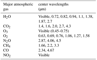
In this paper we focus on gaseous absorption. Aerosol retrieval algorithms (Vermote et al., 1997) tend to use satellite observations taken in wavelength regions where gas absorptions are small. However, while gas absorption is small in these “window” bands, it is not zero. For example, for the 20 nm wide Moderate Resolution Imaging Spectroradiometer (MODIS) band near 0.55 µm, in the middle of the Chappuis region, there is absorption due to ozone. For the US 1976 Standard Atmosphere (US76, 1976), with total column ozone of 344 Dobson units (DU), the gas absorption optical depth (τGAS) is about 0.03 in this band. This is of similar magnitude to pristine AOD (∼ 0.05) and is equal to the required measurement accuracy (GCOS, 2011; GCOS-IP, 2016). Water vapor, measured as precipitable water vapor (PW or w), absorbs as well and introduces even greater uncertainty. For example, the w of the US76 is a modest 1.4 cm, which translates to τ of about 0.025 in the MODIS 2.11 µm band or a τ of 0.05 for a similar-wavelength Visible Infrared Imaging Radiometer Suite (VIIRS) band centered near 2.25 µm. The major difficulty with ozone and water vapor is that the total column burden of these gases varies spatially and temporally over the globe (Hegglin et al., 2014). Other trace gases, including carbon dioxide and methane, also absorb shortwave radiation in wavelength-specific regions. While these gases are more evenly distributed (well mixed) across the globe, failing to correct for their absorption would also lead to errors in aerosol retrieval.
Different aerosol retrieval algorithms respond to the challenge of gaseous correction differently. Some include all gaseous absorbers and account for the variability of water vapor and ozone (Levy et al., 2013, 2015), while others use a fixed ozone concentration (e.g., Thomas et al., 2010; Sayer et al., 2012), and others correct for some gases but consider the effect of other gases to be negligible (MISR ATBD 09, 2008; available at https://eospso.gsfc.nasa.gov/sites/default/files/atbd/atbd-misr-09.pdf, last access: 31 May 2018). Few include methane (Levy et al., 2013, 2015). How does a less complete gaseous correction scheme affect the global retrieval of AOD? How sensitive are gaseous absorption schemes to slight shifts in spectral bands from instrument to instrument? While all operational aerosol retrieval algorithms employ gaseous correction schemes in their retrieval and describe these schemes, more or less, within the “gray literature” of internal documentation, there are few recent articles in the peer-reviewed literature that openly describe the process and quantify the impact of the subtle choices made during algorithm development.
In this paper we re-examine gaseous correction as it is applied in the traditional MODIS dark-target (DT) aerosol retrieval (Levy et al., 2013), and as that retrieval algorithm is ported to the new VIIRS data (Levy et al., 2015). In Sect. 2 we discuss the absorption of radiation by atmospheric gases within the MODIS and VIIRS bands used for the DT aerosol retrieval. We introduce the relationship of gas abundance to its transmittance spectra, which is the theoretical basis for gas corrections in DT AOD retrievals. The atmospheric gas correction methodology is detailed in Sect. 3. The impact of the updated atmospheric gas corrections applied to the Collection 6 MODIS AOD is also briefed in Sect. 3. In Sect. 4 we discuss the importance of accurate atmospheric gas corrections in the context of DT AOD retrievals from the VIIRS instrument. The study is summarized and concluded in Sect. 5.
2.1 The DT aerosol algorithm and wavelength bands
As explained in detail by Levy et al. (2013, 2015) and references therein, the dark-target (DT) aerosol algorithm uses seven channels (or bands) covering the solar reflective spectral region from blue to the shortwave infrared (SWIR) to characterize aerosols, clouds and the Earth's surface. These bands were specifically chosen to correspond to the spectral window regions of minimal gas absorption. On MODIS, these bands include B1, B2, B3, B4, B5, B6 and B7, which are each 20–50 nm in width and centered near 0.65, 0.86, 0.47, 0.55, 1.24, 1.63 and 2.11 µm, respectively. On VIIRS, the DT algorithm uses bands M3, M4, M5, M7, M8, M10 and M11, which are the “moderate-resolution” or M bands with 20 and 60 nm bandwidths, and they are centered near 0.48, 0.55, 0.67, 0.86, 1.24, 1.60 and 2.26 µm, respectively.
The DT algorithm is actually two algorithms, one applied to MODIS- or VIIRS-measured reflectance over land surfaces and the other to measured reflectance over ocean (Levy et al., 2013, 2015). Both the land and ocean algorithms employ a single atmospheric gas correction method before any retrieval is performed. DT uses a lookup table (LUT) approach in which atmospherically corrected observed top-of-atmosphere (TOA) reflectance is compared with simulated reflectance. The simulations are calculated by radiative transfer (RT) codes and account for multiple scattering and absorption effects of a combined surface (land or water), molecular (Rayleigh) and aerosol scene but do not account for gaseous absorption. These simulations also account for the angular dependence of the scattered radiation, through use of a pseudo-spherical approximation (e.g., Ahmad and Fraser, 1991). The DT retrieval operates on regions of pixels for which cloud pixels, glint pixels and other unsuitable pixels have been masked out. Thus, the DT aerosol retrieval is performed for cloud-free sky, and assumptions have been made about the surface reflectance properties and atmospheric constituents. The LUT is interpolated as a function of observing geometry (solar and view zenith and azimuth angles) and then searched to determine which aerosol conditions provide the spectral reflectance that best “matches” the spectral reflectance observed by the satellite. The reported solution (retrieved spectral AOD) is some function of the solutions that meet sufficient criteria for matching the observations. For the DT algorithm, expected uncertainty for retrieved AOD at 0.55 µm (as compared to global network of sun photometers) is ±(0.05 + 15 %) over land and ±(0.03 + 10 %) over ocean (Levy et al., 2013).
These LUTs are created as if the atmosphere were composed only of aerosol and scattering (Rayleigh) molecules. The gas absorption is assumed to be zero. This is because of the large spatial/seasonal variability of two of the primary absorbers: ozone and water vapor. Ozone can range from 100 to 500 DU around the globe (Hegglin et al., 2014), and water vapor varies by an order of magnitude from the wet tropics to the dry poles. It would be cumbersome and computationally inefficient to add two or more new indices to the LUT and cover the dynamic range of each gas in the LUT calculation.
While gas absorption in these window bands may be small, they are not zero, as described above. Figure 1 shows the TOA transmission spectra (black lines) in the 0.4–2.5 µm spectral range in the presence of major gases, including H2O, O3, CO2, CH4, O2, N2O and CO. The transmission spectra of each gas were calculated using the Line-By-Line Radiative Transfer Model (LBLRTM) code (Clough et al., 1992, 2005) for a nadir-viewing geometry and for the US 1976 Standard Atmosphere (1976). A transmittance of 1.0 indicates that the atmosphere is transparent to incoming solar radiation (insolation), i.e., that it is not absorbed in the atmosphere. Overlaid on Fig. 1 are the spectral response functions of the seven MODIS channels (blue curves) and seven VIIRS channels (red curves) used in the DT retrievals. As can be seen from Fig. 1, depending on the wavelength, the atmosphere can be totally transparent to a certain gas and partially opaque to another. For example, in the MODIS 0.62–0.67 µm band (B1), H2O, O3, and O2 absorb radiation, while CO2, N2O, CO and CH4 do not. In the 1.230–1.250 µm band (B5), O2, H2O and CO2 are major absorbers, while other gases are not. Absorption bands of the major atmospheric gases are listed in Table 1.
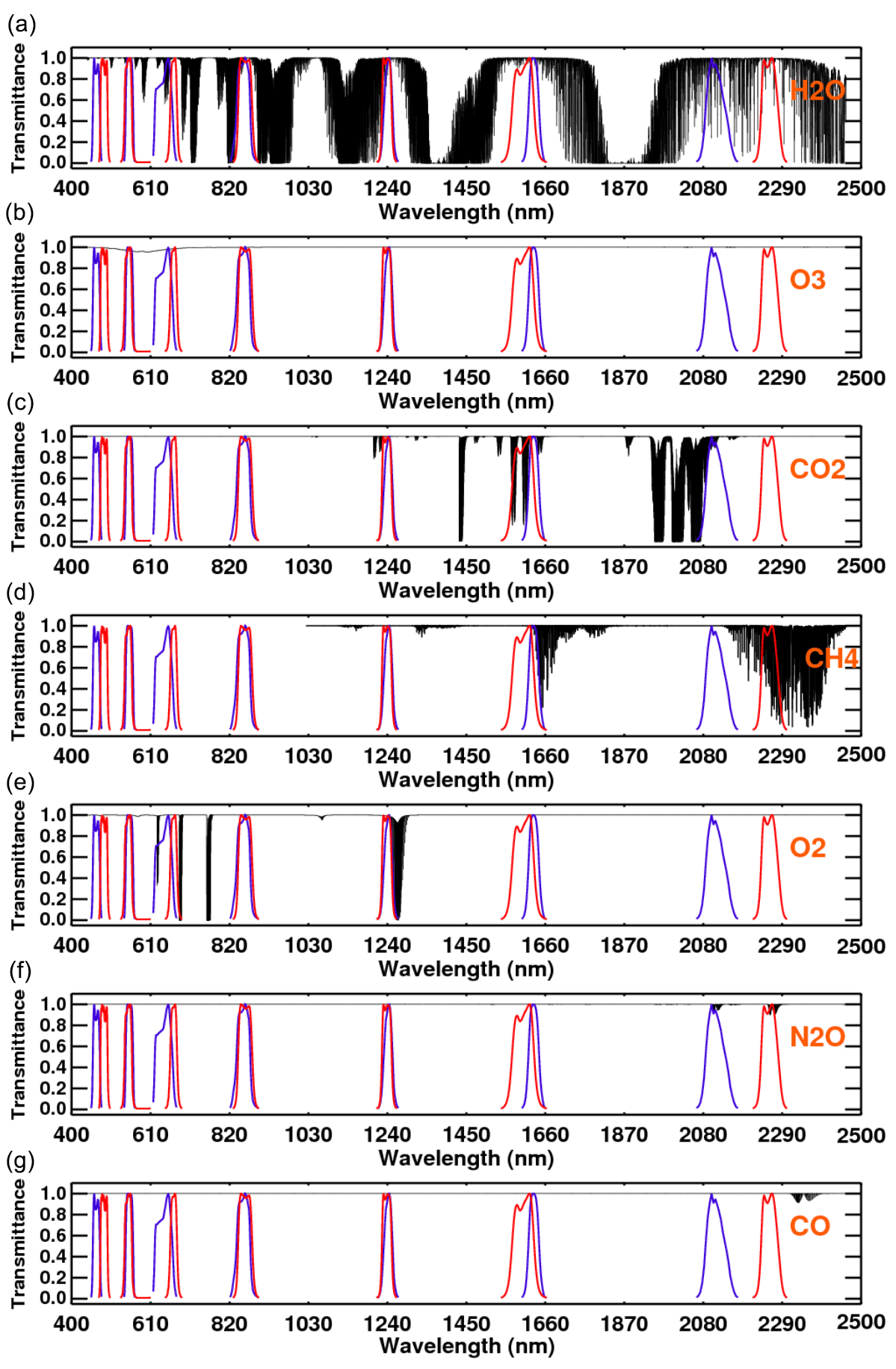
Figure 1The TOA transmission spectra (black) of the major atmospheric gases in the visible and near-infrared part of the electromagnetic spectrum (400–2500 nm). The Line-By-Line Radiative Transfer Model (LBLRTM) was used to calculate these gas spectra for a nadir-viewing geometry and the US 1976 Standard Atmosphere. The spectral response functions of MODIS channels B1–B7 (blue curves) and seven VIIRS channels (red curves) are overlaid to visualize their position in the atmospheric “window” regions where gas absorption effect is minimal.
Note that there are also wavelength regions that are nearly opaque because of gas absorption. For example, Fig. 1 shows the well-known water vapor absorption within the wavelength region near 1.38 µm. Because of the strong absorption, the 1.38 µm band cannot be used for aerosol retrieval. Yet this band is very useful for detecting cirrus clouds that would otherwise contaminate a cloud-free aerosol retrieval (Gao et al., 2002). This special case of using absorption information is not discussed further in this paper.
Table 1Absorption bands of atmospheric gases in visible and near-IR region.
2.2 Derivation of a gas absorption correction
Because the LUT is calculated without gas absorption, an alternative technique must be substituted to account for the effect of the gases in each wavelength. If not, then when the algorithm attempts to match the measured TOA reflectances to the LUT-calculated reflectances the LUT values will be brighter than the measured values for the same amount of aerosol. In the most straightforward sense retrieved AOD, dominated by scattering, will be systematically too low because the retrieval will be searching for a less bright TOA reflectance in the LUT, with less aerosol, to match the observed values. The algorithm deals with this mismatch between measured and LUT reflectance caused by the missing gas absorption in the LUT values by adjusting the measured TOA reflectances in each wavelength band, in effect brightening the measurements to better match the values in the LUT.
Figure 1 shows that six gases (H2O, O3, CO2, N2O, O2 and CH4) have absorption lines that fall within the wavelength bands used for the DT aerosol retrieval. Because each window band spans tens of nanometers, every DT channel is affected by at least one gas where the transmittance is less than 1.0.
We have introduced two measures, gas opacity and transmissivity corresponding to the gas absorption optical depth and transmittance. The two parameters are related via
where is the downward transmittance for a particular wavelength band (or λ) and for a particular absorbing gas “i”; is the gas optical depth designated for the particular gas and wavelength; and Gi is the air mass factor (or the atmospheric path length, i.e., the slant path through the atmosphere) for gas i. Equation (1) shows that transmission of light is a function of the air mass factor (Gi) and the gas optical depth , and that transmissivity decreases with increasing air mass and increasing gas concentration.
2.2.1 Gas optical depth
The gas optical depth, , represents the spectral integral over the wavelength band; if the gas concentration is uniform along the path (column), then will be directly proportional to the loading of gas i in the column. Some gases are indeed well mixed in the atmosphere, but water vapor and ozone are not. These important absorbers exhibit distinctive vertical profiles, as will be discussed in Sect. 3.1. Note that each individual gas has its own particular absorption efficiency based on its characteristic absorption cross section and that for the same column concentrations will be different for different gases. In the absence of a long slant path, and for small gas optical depths ( ≪ 1.0), transmission can be estimated by .
2.2.2 Air mass factor
The air mass factor, G, can be approximated as , where Z is the zenith angle for a homogenous (exponential decay) atmosphere and for small values (near nadir) of Z. This is the flat-Earth approximation. As Z increases beyond 60∘, the air mass factor is more accurately described by spherical shell geometry towards the horizon (Gueymard, 1995), i.e.,
where ; RE= radius of Earth (6371 km); and Hatm= effective scale height of the atmosphere (ca. 9 km). This expression accounts for Earth's sphericity and atmospheric refraction. Differences in computing G are small for Z < 70∘ but increase to 10 % as Z= 84∘ (the maximum zenith angle allowed within the DT algorithm).
Yet there are complications. When atmospheric constituents are well mixed and their concentrations are nearly proportional to altitude within the atmosphere, Eq. (2) is sufficient. However, water vapor (concentrated near the surface) and ozone (concentrated in the stratosphere) are not well mixed in the vertical, having different scale heights. In this layered situation (rather than continuous), there are empirical formulas (e.g., Kasten and Young, 1989) that provide slight improvements to the calculation of G assuming spherical geometry. For example, Gueymard (1995) derived the empirical formula
where ai,j are the coefficients () for gas type i. Thus, Gi varies with gas type and specific profile within the atmosphere. The values of coefficients ai,j can be found in Table 4.1 of Gueymard (1995).
As long as the total gas optical depth is small (, the total transmission of all trace gases is well approximated by the product of each individual gas:
The total gas transmissivity defined in Eq. (4a) for each wavelength band quantifies the degree to which the measured reflectance will be diminished due to gaseous absorption. In order to match the measured reflectances to those calculated for the LUT, these diminished reflectances have to be “corrected” or brightened. This correction factor is simply the inverse transmissivity (),
which, when multiplied with the measured reflectance, restores the amount of light absorbed by gases along the one-way path of transmission. Or, given a measured radiance, LM, the corrected (brightened) radiance L is simply .
When observing from a ground-based sun photometer (e.g., AERONET), the correction is straightforward, because the path of transmission traverses the depth of the atmosphere only once. The problem is more complicated for satellite remote sensing, because a satellite measures radiation that has traveled downwards through the atmosphere and then back up to space. We have to calculate a two-way correction factor, and G must account for the Z angles of both downward (the solar zenith angle) and upward paths (view zenith). As Z gets large, the vertical profile of the gas (layering) becomes more important.
There are two parameters determining the transmission, , and therefore the correction factor, , and these are Gi and . The goal, then, is to parameterize Eqs. (4a) or (4b), i.e., the relationship between atmospheric transmission of gas and , taking into consideration the varying gas concentrations and their vertical profiles through the atmosphere around the globe. Furthermore, the parameterization will be developed to link directly to column measures of the gases instead of to the optical depth. This allows the algorithm to bypass calculations of optical depth from inputs of precipitable water vapor (w in centimeters) and ozone (O in Du), and instead use the inputs directly.
To develop an empirical relationship between atmospheric gas transmission, the air mass factor (Gi) and its optical depth (), we require a radiative transfer (RT) code that can accurately simulate the gaseous absorption and transmission process in the atmosphere. Among other things, the RT code requires these two pieces of information: (a) the absorption cross sections and concentration of gas constituent in spectral bands of interest and (b) accurate high-resolution information of the absorption spectra of the relevant gases. The MODIS and/or VIIRS channels widths are on order of 20–50 nm. We require a high-resolution database to capture the fine absorption lines within these bandwidths. To address (a) and (b), we use the LBLRTM to parameterize Eqs. (4a) and (4b) instead of a MODerate resolution atmospheric TRANsmission (MODTRAN)-based RT code. The following section provides details of LBLRTM.
3.1 LBLRTM description
The LBLRTM is known to be an accurate and flexible radiative transfer model that can be used over the full spectral range from ultraviolet to microwave (Clough et al., 2005). It uses the High-resolution TRANsmission (HITRAN) molecular absorption database (Rothman et al., 2009) to calculate transmittance and radiance of molecular species. The HITRAN2008 database contains over 2 713 000 lines for 39 different molecules. The spectral resolution of the data is different in different spectral regions and for different species (see Rothman et al., 2009). For example, for water vapor absorption in the near-IR region, the line resolution is 0.001 cm−1 (2.5–3.4 mum). The LBLRTM has been extensively validated against atmospheric radiance spectra (e.g., Turner et al., 2003; Shephard et al., 2009; Alvarado et al., 2013). Use of the HITRAN database and other attributes of LBLRTM provides spectral radiance calculations with accuracies that are consistent with validation data. Limiting errors are, in general, attributable to line parameters and line shape. Algorithmic accuracy of LBLRTM is approximately 0.5 % and is about 5 times less than the error associated with line parameters (Clough et al., 2005).
3.2 LBLRTM calculations for MODIS and VIIRS
The LBLRTM model was run for many scenarios representing different combinations of gas vertical profiles, gas concentrations and air mass factors for each type of gas and each of the wavelength bands of interest. Transmissions of the 10 important atmospheric gases – viz. H2O, O3, O2, N2O, NO2, NO, SO2, CO2, CO and CH4 – that affect either the MODIS or the VIIRS spectral bands (Levy et al., 2013) were calculated. However, only H2O, O3, CO2, N2O, O2 and CH4 were found to have some absorption in the wavelength bands used for the DT aerosol retrieval (Tables 2 and 3). The results link transmission () or gas correction factor () to gas path length: for water vapor (H2O) and O for ozone (O3), where w is the precipitable water vapor in centimeters and O is ozone column loading in DU. Values for w and O are input into the algorithm from ancillary data. The other gases are considered to be well mixed and not varying spatially or temporally and therefore are not dependent on input ancillary data. The final parameterization will be curve fits through the scatter of the model results.
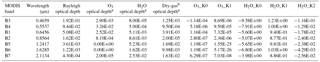
Table 2Optical depth of major atmospheric gases in seven MODIS channels.
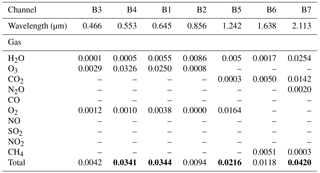
Bold values show channels where total gas optical depth ≥ 0.02 to put in context the requirement of aerosol optical depth accuracy of better than 0.02.
Table 3Optical depth of major atmospheric gases in seven VIIRS channels.
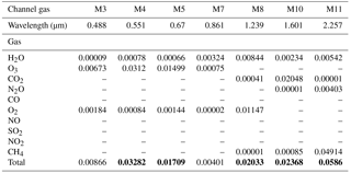
Bold values show channels where total gas optical depth ≥ 0.02 to put in context the requirement of aerosol optical depth accuracy of better than 0.02.
As described in Sect. 2.2, will be affected by the vertical distribution of the gases in the column, especially at oblique zenith angles. To account for this effect in building the parameterization, we use 52 atmospheric profiles (Pubu Ciren, NOAA, Chevallier, personal communication, 2002) that were obtained from model runs and characterize different locations and seasons (Fig. 2). The columnar gas concentrations differ across the 52 profiles, varying by more than a factor of 10 for water vapor and by 100 % for ozone. Except for NO2, which is highly variable in both the horizontal and vertical, the other trace gases tend to be well mixed throughout the atmosphere. Using radiative transfer calculations, Ahmad et al. (2007) show that NO2 has the largest impact (1 %) on TOA reflectance in the blue channels (412 and 443 nm). Other visible channels are impacted to a lesser degree. We will use the term “dry gas” to denote the eight gases that are neither H2O or O3 and use the US 1976 Standard Atmosphere as a default profile.
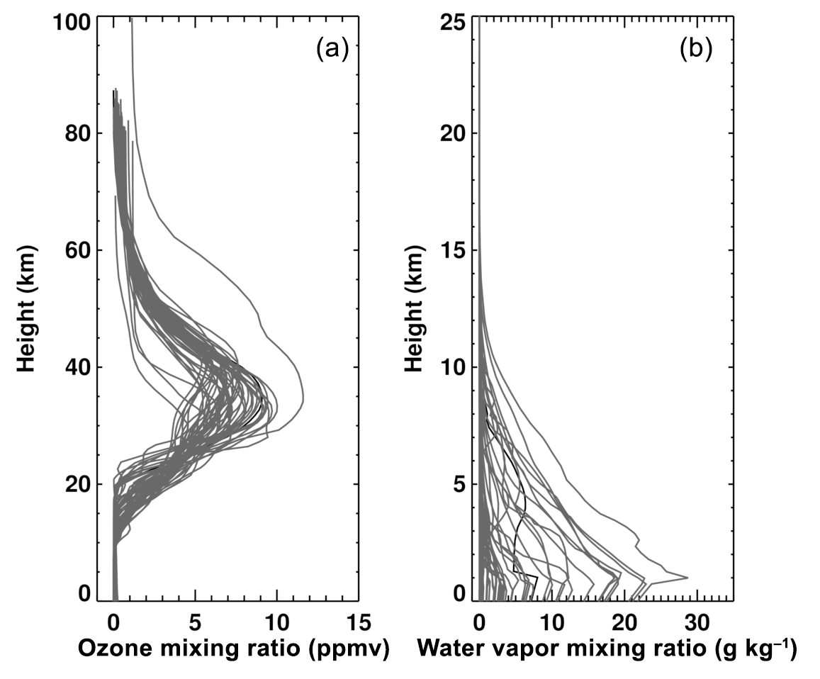
Figure 252 different ECMWF profiles for (a) ozone and (b) water vapor used in the Line-By-Line Radiative Transfer Model to calculate the respective gas transmittance.
For H2O and O3, and each of their respective profiles, we use LBLRTM to calculate air mass factors and transmissions for 10 values of viewing zenith angle, ranging from 0 to 80∘. Transmission is integrated across the wavelength band and weighted by relative sensor response (RSR) (Barnes et al., 1998; Xiaoxiong et al., 2005) within the band. Because air mass factor (Gi) varies with gas type (on account of the vertical profile), LBLRTM calculates Gi as well as transmission for the given column amount of gas i. For dry gas, the integrated RSR weighted transmission is converted to gas optical depth, so dry-gas transmission (as a function of air mass factors) is easily computed using Eq. (1). The US76 profiles are used to compute dry-gas transmission for nadir view.
Figure 3 plots the relationship between absorption correction factor, , and gas path length, , for H2O (a) and O for O3 (b), for MODIS. Figure 4 plots the same for VIIRS. These correction factors (inverse of transmission) are plotted for each window band, for different combinations of H2O or O3 concentrations (w in cm or O in DU) and internally derived air mass factors (Gi) for the given gas type and specific vertical profile. Water vapor, being so variable as well as concentrated near the boundary layer, cannot be explained with a linear relationship. However, for water vapor (Figs. 3a and 4a), a near-linear dependence of to does exist in log–log space. Nevertheless, even within the log–log space, there is a small curvature that required a quadratic empirical fit. For ozone, however, the log of our correction factor ( is nearly linear as a function of absorption through a slant path (. Again, note that Gi is computed by LBLRTM and represents the curvature and vertical profile of each gas type.
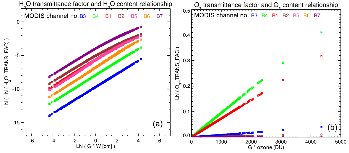
Figure 3Relationship between gas transmittance factor and gas content in the MODIS channels B1–B7: (a) for H2O and (b) for O3. Gas content is scaled by the air mass factor (G). Gas transmittance was calculated for 52 water vapor and ozone profiles (varying gas concentration) and 10 viewing zenith angles (air mass factors) ranging from 0 to 80∘. These wavelength-dependent empirical relationships are used by the DT aerosol retrieval algorithm for atmospheric gas corrections.
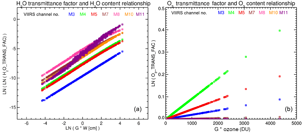
Figure 4Relationship between gas transmittance factor and gas content in the seven VIIRS channels: (a) for H2O and (b) for O3. Gas content is scaled by the air mass factor (G). Gas transmittance was calculated for 52 water vapor and ozone profiles (varying gas concentration) and 10 viewing zenith angles (air mass factors) ranging from 0 to 80∘. These wavelength-dependent empirical relationships are used by the DT aerosol retrieval algorithm for atmospheric gas corrections.
Equation (5) describes the quadratic empirical relationship (seen in Figs. 3a and 4a) between the gas transmission correction factor of water vapor (, its concentration (w) and the air mass factor (:
Equation (6) describes the near-linear relationship for ozone (Figs. 3b and 4b):
“O” denotes ozone concentration in Eq. (6), and is the air mass factor for ozone and is computed using Eq. (3).
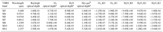
The regression coefficients , and as well as and (the slopes and intercepts) for H2O and O3 are presented for MODIS and VIIRS in Tables 4 and 5. The slope and intercepts are wavelength dependent (lines of different color on Figs. 3 and 4) and in accordance with absorption characteristics of the gas. For example Table 2 shows that water vapor absorption is the highest in MODIS band 7 (B7 = 2.11 µm) and lowest in B3 (0.47 µm). Correspondingly, the slope and intercept for the H2O regression relation (Table 4) indicates the largest water vapor correction in B7 and the lowest in B3. Similarly, largest correction (and slope) for ozone is in MODIS B4 (0.55 µm) and lowest in B7.
Table 4Gas absorption coefficients and climatology for MODIS.
a For each MODIS band, this nadir-looking (viewing
zenith angle = 0) optical depth for the gas is computed from the US 1976
Standard Atmosphere
in LBLRTM.
b Dry gas includes CO2, CO, N2O,
NO2, NO, CH4, O2, SO2.
Table 5Gas absorption coefficients and climatology for VIIRS.
a For each VIIRS band, this nadir looking (viewing
zenith angle = 0) optical depth for the gas is computed from the US 1976
Standard Atmosphere
in LBLRTM.
b Dry gas includes CO2, CO, N2O,
NO2, NO, CH4, O2, SO2.
To calculate the correction factors for water vapor ( and ozone (, Eqs. (5) and (6) require information on water vapor (w) and ozone concentration (O). For the DT algorithm, these are provided by an ancillary data set. For the current version (e.g., MODIS Collection 6), ancillary data are acquired from National Center for Environmental Prediction (NCEP) analysis, specifically the “PWAT” and the ozone fields from the 1∘ × 1∘ global meteorological analysis (created every 6 h – format “gdas.PGrbF00.YYMMDD.HHz”). Note that there are water vapor products derived operationally from MODIS and VIIRS data (e.g., Gao and Goetz, 1990; Kaufman and Gao, 1992). However, the DT aerosol algorithm runs before these other algorithms in the processing chain, causing the internally derived water vapor to be unavailable to the aerosol algorithm in real-time processing and, thus, the reliance on ancillary data.
In case the ancillary information is not available, the gas absorption can still be estimated. Either a forecast field (e.g., Global Data Assimilation System (GDAS) forecast) or a “climatology” can be used. For example, if the US76 is assumed as the climatology for gas profiles, then τi for that gas is given in Tables 4 and 5. In this case, we use Eqs. (7) and (8) to calculate correction factors for water vapor and ozone, respectively:
where and are the climatological mean values of gas optical depth for water vapor and ozone, respectively.
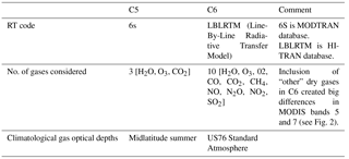
Table 6Atmosphere gas correction table differences: C5 vs. C6.
is the correction factor due to dry gas, which includes CO2, CO, N2O, NO2, NO, CH4, O2, SO2 and other trace gases in LBLRTM calculations. For the DT retrieval bands only CO2, N2O, CH4 and O2 contribute to absorption (Tables 2, 3). Since the gases are generally well mixed throughout the entire atmosphere and do not experience day-to-day changes, we only consider the climatological mean of the total optical depth of the combined dry gases and compute its transmittance factor as follows:
Figure 5 presents the gas optical depth for the US76, for the MODIS bands and corresponding VIIRS bands. In some cases (e.g., B4 vs. M5), the differences are small. In other cases (e.g., B5 vs. M8), the total optical depth may be similar, but the relative contribution between different gases is different. Finally, in at least one set of bands (B7 vs. M11), both the total optical depth and the relative contributions between gases is very different. The US76 is a case with a small amount of water vapor (w= 1.4 cm), but one can see how quadrupling the w (e.g., as in a tropical atmosphere) would greatly change the relative correction needed for B7 vs. M11, or even B1 vs. M5.
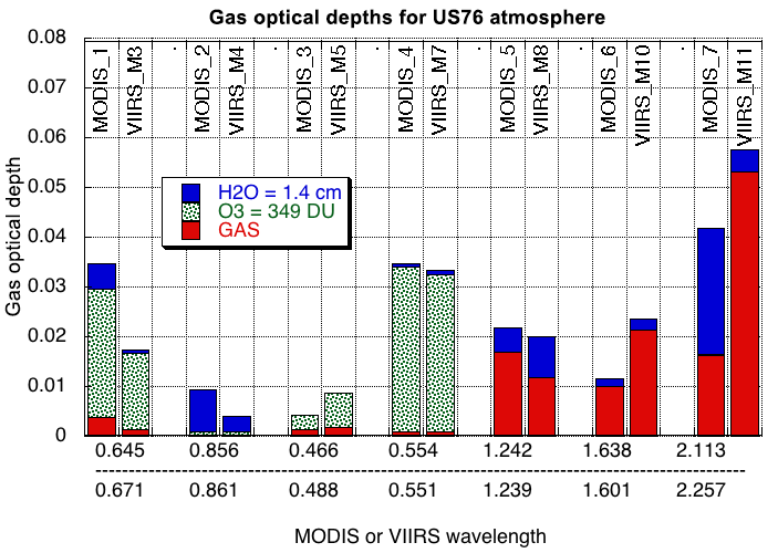
Figure 5Comparison of gas optical depths calculated for the US 1976 Standard Atmosphere using MODIS C6 and VIIRS gas correction coefficients. Different colors represent constituent gases (H2O is blue O3 is green hatched and “dry” gas is red). Large differences in gas optical depths are seen in MODIS channels 1, 2, 6 and 7.
3.3 Application within the DT algorithm.
Whether using climatology for water vapor and ozone columns, or using the estimates from a meteorological assimilation system (e.g., GDAS for the current DT algorithm), we need to correct for the combined absorption of all gases. The total gas absorption correction term, , is the product of individual gas corrections, that is,
The MODIS DT aerosol retrieval algorithm ingests calibrated and geolocated MODIS-measured reflectance data, known as the Level 1B (L1B) product. The corresponding VIIRS DT algorithm ingests a similar VIIRS-measured product. This measured reflectance ( is corrected for atmospheric water vapor, ozone and dry gas, using the correction factors derived above for each wavelength band:
where ρλ is the corrected or brightened reflectance that can now be used to compare with the calculated TOA reflectances of the LUT, as described in Sect. 2.2. Note that this spectral reflectance, ρλ, represents the combination of Rayleigh (molecular scattering) plus aerosol in the atmosphere. It also includes contributions from Earth's surface (land or water).
The gas absorption correction methodology is the same whether performed for MODIS or VIIRS. In fact, the equations (Eqs. 5–11) have remained the same throughout all versions of the DT algorithm. As our ability to characterize absorption lines as well as the spectral response of the sensor has improved, it is the coefficients of the equations that have evolved. When the DT algorithm was updated from Collection 5 (C5) to Collection 6 (C6), the underlying gas absorption corrections became more sophisticated (Levy et al., 2013). This is represented in Table 6. The primary differences between C5 and C6 are that the HITRAN database in LBLRTM is used in C6 instead of the MODTRAN parameterization available in 6S that was used in C5, and that additional dry gases have been included in C6's correction. These changes made a difference. The latest version of aerosol data from DT is Collection 6.1, which uses the same gas absorption corrections as C6. As the DT algorithm is ported from MODIS to VIIRS data, the quality of gas correction will also make a difference.

Figure 6(a) shows the spatial distribution of gridded L2 reflectance in seven VIIRS channels (i.e., M3, M4, M5, M7, M8, M10, M11) for July 2013. (b) shows the spatial distribution of the difference between VIIRS reflectance obtained by applying VIIRS gas correction coefficients and MODIS C6 gas correction coefficients in seven VIIRS channels (i.e., M3, M4, M5, M7, M8., M10, M11) for July 2013. This panel demonstrates the impact of using MODIS gas correction on VIIRS reflectance used for retrieving aerosol optical depth.
The DT retrieval is based on a LUT approach wherein the measured and modeled spectral reflectance is matched for inversion. Any change affecting the calculation of gas-corrected spectral reflectance will subsequently affect the retrieved AOD. Levy et al. (2013) showed the impact of using the updated atmospheric gas corrections on MODIS C6 AOD retrievals. This led to higher AODs globally. Over land (ocean), the 0.55 µm global mean AOD differed by ∼ 0.02 (0.007). The large (> 0.02 regionally) change over land was primarily due to a larger gas correction in the 1.24 µm MODIS B5 band (see Fig. A2 in Levy et al., 2013), which in turn increased the reflectance in B5, and the subsequent estimate of the normalized difference vegetation index in the SWIR channels (B5 vs. B7) used to estimate surface reflectance in other bands (Levy et al., 2010). The stronger gas correction in B5 came from including the O2 absorption, which had not been accounted for in C5 (see Table 2). Interestingly, Levy et al. (2013) noted that, while the overall correction in B7 (2.11 µm) remained similar, the relative weightings of dry gas and H2O was revised.
Even though the MODIS and VIIRS instruments have similar channels, the MODIS gas correction coefficients cannot be applied to aerosol retrievals from VIIRS observations. The slight differences in the bandwidth and channel's central wavelengths (see Fig. 5) will compromise the accuracy of aerosol retrievals. For example, as compared with MODIS B7 (2.11 µm), the VIIRS M11 (2.25 µm) band has less absorption from H2O. However, MODIS B7 lies in a CO2 absorption band, while VIIRS M11 lies in a region of CH4 absorption. Although the CH4 optical depth in VIIRS M11 is small (∼ 0.03), it will affect the dark-target retrievals in the same way as O2 inclusion affected C6 retrievals (when compared to C5).
As a perturbation experiment we intentionally apply the MODIS gas corrections to the VIIRS observations, even though we know this to be incorrect. Figure 6a plots the spatial distribution of spectral TOA reflectance after applying VIIRS-appropriate gas corrections. It shows the mean monthly TOA reflectance for VIIRS. Figure 6b is the reflectance differences between applying VIIRS-appropriate gas corrections and MODIS gas corrections to VIIRS observations. From top to bottom, we find a mean difference of 0, −0.5, −6.6, −2.7, −1.5, 3.2 and 5.3 %, respectively, in VIIRS channels M3, M4, M5, M7, M8, M10 and M11. Looking back at Fig. 5, one can see that for example, by using proper M5 assumptions instead of the B1 MODIS assumptions, we now apply only about half the correction as before, resulting in a 6.6 % reduction of reflectance. Channel M7, with about 50 % less water vapor correction (see Fig. 5), results in 2.7 % lower reflectance. Larger gas corrections owing to CO2 absorption in M10 and CH4 absorption in M11 (Fig. 5) result in positive bias in M10 and M11 reflectance values globally.
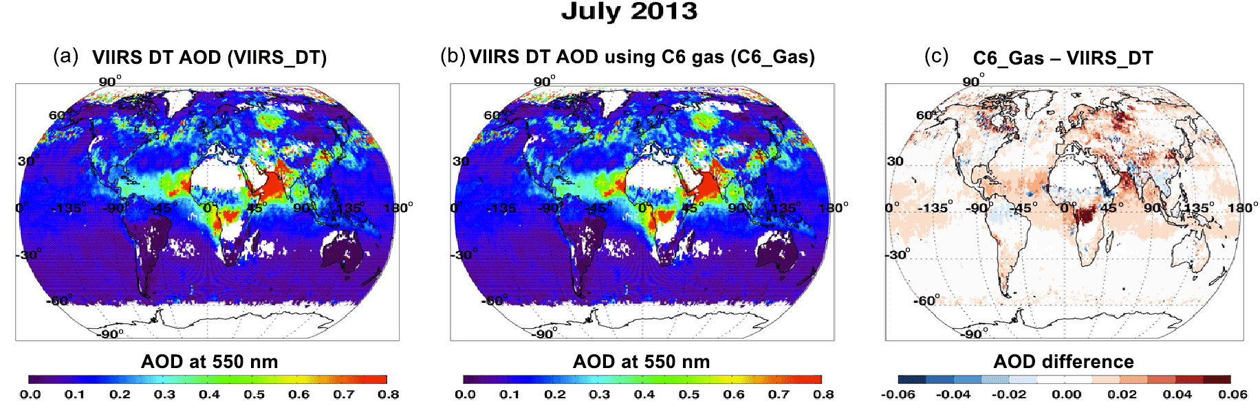
Figure 7Impact of updated atmospheric corrections on VIIRS AOD (550 nm) retrieval. All things being equal, using the C6 aerosol DT retrieval algorithm (a) is AOD using atmospheric coefficients calculated for VIIRS bands, and (b) is AOD using C6 atmospheric corrections; (c) is the difference between (b) and (a). The global mean AOD differs by ∼ 0.012 over land and by ∼ 0.004 over ocean. Difference are larger than these mean values regionally but < 0.08. Differences are mostly positive (reds) except in some desert/bright regions where some negative differences appear.
Now, we continue the perturbation experiment and test the impact of slight differences in the band positioning between MODIS and VIIRS on AOD retrieval by performing two sets of retrievals. The first set (a) is as if we had applied appropriate VIIRS band corrections, while the second (b) is as if we had simply (naively) applied MODIS (C6) coefficients to VIIRS data. Figure 7 shows the AOD retrieved from these two cases (a and b) for an entire month (July 2013) of VIIRS data. While general AOD spatial patterns are in agreement, panel c shows differences in AOD of up to 0.07 between the two retrievals. Clearly, naively applied MODIS gas corrections to VIIRS data would lead to a global mean AOD underestimate of ∼ 0.01 for July 2013. While these differences are within the global uncertainties for AOD (e.g., GCOS), the regional differences can be much larger.
Although once considered to be trivial in magnitude, accurate atmospheric gas corrections have become more important as we strive towards better accuracies in AOD products and towards a seamless climate data record. It is noteworthy that the gas absorption spectra of Fig. 1 have been updated several times in recent years (Alvarado et al., 2013) as the scientific community continues to engage in study of gas absorption lines with improved instrumentation and gas spectroscopic measurements. Changing gas absorption spectra will affect the channels designed for new remote-sensing instruments and in understanding how these lines might affect the retrieval of proposed geo-physical products. Every instrument design involves characterization of channel bandwidths and the spectral response functions of the instrument's channels. This aptly calls for updates in modeling the absorption by gases in the channels used for aerosol retrievals. For the MODIS Collection 6 AOD product, the team switched from using a MODTRAN gas spectroscopic database to the HITRAN spectroscopic database and found differences.
Performing aerosol optical depth retrieval, from satellite measurements, requires extracting the aerosol signal from the total radiance measured by the sensor at the top of the atmosphere. The total radiance includes signal from the underlying surface and from atmospheric constituents such as gases, clouds and aerosols. In this paper, we have described the physics and methodology employed by the dark-target aerosol retrieval algorithm for atmospheric gas correction of the cloud-free radiance measurements from the MODIS and VIIRS sensors. We have shown that the empirical correction applied to one sensor (MODIS) cannot be applied to another sensor (VIIRS) even when the channels of the two sensors may be similar. For a specific month of VIIRS observations (July 2013), not accounting for the sensor's bandwidth and positioning of its central wavelength in the electromagnetic spectrum, can result in an AOD retrieval bias of about 0.01 (global average) and up to 0.07 at regional scales.
Water vapor, ozone and carbon dioxide are the major absorbers of solar radiation. Historically, they have been accounted for in atmospheric gas corrections by aerosol retrieval algorithms. However, until recently, standard routine algorithms (e.g., the DT algorithm used on MODIS) did not consider other gases. For example, oxygen with a gas optical depth of about 0.016 is important in MODIS B5 band (1.24 µm) (Levy et al., 2013). Methane is an important absorber in band M11 (2.25 µm) of VIIRS with an optical depth of ∼ 0.05. Starting with MODIS Collection 6, and the DT algorithm ported to VIIRS, four additional atmospheric gases (N2O, CH4, O2, SO2) are addressed by the gas correction in these DT algorithms.
For the dry-gas component, the DT gas correction assumes a homogeneous global distribution spatially and a US76 type of vertical distribution for the eight gases. Carbon dioxide, oxygen, nitrous oxide and methane are major absorbers in our dry-gas category. Except for NO2, which is highly variable in both the horizontal and vertical, the other gases tend to be well mixed throughout the atmosphere. Spatial variability of well-mixed gases is typically around 10 %, is mostly latitudinal and is smaller than seasonal variability (e.g., see methane maps here: http://www.temis.nl/climate/methane.html, last access: 31 May 2018). For the nadir view, a 10 % error due to spatial variability will only introduce an error of 0.005 in the methane correction (optical depth ∼ 0.05 in VIIRS channel M11). For now, this is a small uncertainty in the overall retrieval. However, as requirements for aerosol retrieval accuracies tighten, even these well-mixed dry gases will require removal of any seasonal and regional biases by using ancillary measurements of these gases or at least seasonal global climatology of gas optical depths, instead of a single climatological value for the entire globe.
Since the DT algorithm corrects for H2O and O3 using ancillary data at every 1∘ × 1∘ grid box, spatial and seasonal variability of these gases is being accounted for. However, the ancillary data have their own uncertainties that propagate into the gas correction and aerosol retrieval. The dark-target team is working towards estimating the error in per-pixel AOD retrievals introduced from several error sources including the errors in H2O and O3 ancillary data (GDAS) used for atmospheric gas corrections. Preliminary analysis suggests (not shown here) that gas corrections errors, stemming from considering 20 % errors in ancillary data, are much smaller (more than an order of magnitude) than errors from surface albedo uncertainty, aerosol model selection, spatial heterogeneity in a scene, calibration and cloud contamination errors. This is a work in progress and subject to future publication.
The VIIRS instrument on board Suomi-NPP is a follow-on of the MODIS instrument on Terra and Aqua satellites. While the dark-target team strives to create a seamless climate data record (CDR) of AOD from MODIS and VIIRS, it requires a consistency in AOD retrieval of about 0.02. Any compromise with the accuracy of AOD retrieved from either sensor will impact the CDR consistency requirement. To strive toward these requirements, we cannot ignore quality atmospheric gas corrections in AOD retrievals, and we will update the gas correction factors for each instrument as the community updates the gas absorption database.
As we move into an era of new aerosol missions, revisiting and updating gas corrections in a state-of-the-art algorithm become as important as improving upon other factors (e.g., better surface characterization, cloud clearing, aerosol properties) that affect the AOD retrieval. The dark-target algorithm software has now been generalized to retrieve AOD from sensors other than MODIS and VIIRS. It will be necessary to accurately characterize gases from such current and future instruments as Himawari and GOES-R, among others.
L1B radiance data from VIIRS Suomi-NPP, made available by the Wisconsin-PEATE (now SIPS) team (IFF data), were used to create the MODIS-like C6 aerosol retrievals using the VIIRS DT algorithm. Ancillary data (water vapor and ozone content) from NCEP analysis are used by the DT retrieval algorithm for atmospheric gas correction. The 52 ECMWF water vapor and ozone profiles, used for calculating the transmittance from LBLRTM, were obtained from Pubu Ciren from NOAA (pubu.ciren@noaa.gov).
The authors declare that they have no conflict of interest.
This research work was funded under NASA's grants for MODIS and VIIRS
dark-target aerosol retrieval for the MODIS science team. We are thankful to
Matthew J. Alvarado (from Atmospheric and Environmental Research) for
promptly helping with all our queries related to the LBLRTM. We thank Pubu
Ciren for providing us with the atmospheric profiles for gases and for
knowledge transfer on its use in LBLRTM for calculating NOAA VIIRS
atmospheric gas corrections in aerosol retrievals. We thank Lorraine Remer
for providing us with scientific comments and for editing the
paper.
Edited by: Thomas Eck
Reviewed by: Adam Povey and one anonymous referee
Ahmad, Z., and Fraser, R. S.: An iterative radiative transfer code for ocean-atmosphere systems, J. Atmos. Sci., 39, 656–665, https://doi.org/https://doi.org/10.1175/1520-0469(1982)039<0656:AIRTCF>2.0.CO;2, 1982.
Ahmad, Z., McClain, C., Herman, J., Franz, B., Kwiatkowska, E., Robinson, W., Bucsela, E., and Tzortziou, M.: Atmospheric correction for NO2 absorption in retrieving water-leaving reflectances from the SeaWiFS and MODIS measurements, Appl. Opt., 46, 6504–6512, 2007.
Alvarado, M. J., Payne, V. H., Mlawer, E. J., Uymin, G., Shephard, M. W., Cady-Pereira, K. E., Delamere, J. S., and Moncet, J.-L.: Performance of the Line-By-Line Radiative Transfer Model (LBLRTM) for temperature, water vapor, and trace gas retrievals: recent updates evaluated with IASI case studies, Atmos. Chem. Phys., 13, 6687–6711, https://doi.org/10.5194/acp-13-6687-2013, 2013.
Barnes, W. L., Pagano, T. S., and Salomonson, V. V.: Pre-launch characteristics of the Moderate Resolution Imaging Spectroradiometer (MODIS) on EOS AM-1, IEEE T. Geosci. Remote, 36, 1088–1100, 1998.
Bevan, S. L., North, P. R. J., Los, S. O., and Grey, W. M. F.: A global dataset of atmospheric aerosol optical depth and surface reflectance from AATSR, Remote Sens. Environ., 116, 199–210, https://doi.org/10.1016/j.rse.2011.05.024, 2012.
Boucher, O., Randall, D., Artaxo, P., Bretherton, C., Feingold, G., Forster, P., Kerminen, V.-M., Kondo, Y., Liao, H., Lohmann, U., Rasch, P., Satheesh, S. K., Sherwood, S.,Stevens, B., and Zhang, X. Y.: Clouds and Aerosols, in: Climate Change 2013: The Physical Science Basis, Contribution of Working Group I to the Fifth Assessment Report of the Intergovernmental Panel on Climate Change, edited by: Stocker, T. F., Qin, D., Plattner, G.-K., Tignor, M., Allen, S. K., Boschung, J., Nauels, A., Xia, Y., Bex, V., and Midgley, P. M., Cambridge University Press, Cambridge, United Kingdom and New York, NY, USA, 2013.
Chevallier, F.: Sampled database of 60-level atmospheric profiles from the ECMWF analyses, NWP SAF Report No. NWPSAF-EC-TR-001, available at: http://www.ecmwf.int/publications/ (last access: 31 May 2018), 2002.
Clough, S. A., Iacono, M. J., and Moncet, J.-L.: Line-by-Line calculations of atmospheric fluxes and cooling rates: application to water vapor, J. Geophys. Res.-Atmos., 97, 15761, https://doi.org/10.1029/92JD01419, 1992.
Clough, S. A., Shephard, M. W., Mlawer, E. J., Delamere, J. S., Iacono, M. J., Cady-Pereira, K., Boukabara, S., and Brown, P. D.: Atmospheric radiative transfer modeling: a summary of the AER codes, J. Quant. Spectrosc. Ra., 91, 233–244, https://doi.org/10.1016/j.jqsrt.2004.05.058, 2005.
Denman, K. L., Brasseur G., Chidthaisong, A., Ciais P., et al.: Couplings between changes in the climate system and biogeochemistry, in: Climate Change 2007: The Physical Science Basis, Contribution of Working Group I to the Fourth Assessment Report of the Intergovernmental Panel on Climate Change, edited by: Solomon, S., Qin, D., Manning, M., Chen, Z., Marquis, M., Averyt, K. B., Tignor, M., and Miller, H. L., Cambridge University Press, Cambridge, United Kingdom and New York, NY, USA, 499–587, 2007.
Deuzé, J. L., Herman, M., Goloub, P., Tanré, D., and Marchand, A.: Characterization of aerosols over ocean from POLDER/ADEOS-1, Geophys. Res. Lett., 26, 1421–1424, 1999.
Gao, B. C. and Goetz, A. F. H.: Column Atmospheric Water Vapor and Vegetation Liquid Water Retrievals From Airborne Imaging Spectrometer Data, J. Geophys. Res., 95, 3549–3564, 1990.
Gao, B. C., Kaufman, Y. J., Tanré, D., and Li, R.-R.: Distinguishing tropospheric aerosols from thin cirrus clouds for improved aerosol retrievals using the ratio of 1.38-µm and 1.24-µm channels, Geophys. Res. Lett., 29, 1890, https://doi.org/10.1029/2002GL015475, 2002.
GCOS: Systematic observation requirements for satellite-based products for climate, 2011 update, WMO GCOS Rep. 154, New York, USA, 127 pp., 2011.
GCOS-IP 2016: GCOS Implementation Plan 2016, GCOS-200, available at: https://library.wmo.int/opac/doc_num.php?explnum_id=3417 (last access: 31 May 2018), 2016.
Gueymard, C.: SMARTS2: a simple model of the atmospheric radiative transfer of sunshine: algorithms and performance assessment, Florida Solar Energy Center, 1–78, 1995.
Hegglin, M. I., Fahey D. W., McFarland, M., Montzka S. A., and Nash, E. R.: Twenty questions and answers about the ozone layer: 2014 Update, in: Scientific Assessment of Ozone Depletion: 2014, World Meteorological Organization Global Ozone Research and Monitoring Project – Report No. 55, available at: http://www.esrl.noaa.gov/csd/assessments/ozone/2014/twentyquestions/ (last access: 31 May 2018), 2014.
Herman, J. R., Bhartia, P. K., Torres, O., Hsu, C., Seftor, C., and Celarier, E.: Global distribution of UV-absorbing aerosols from Nimbus 7/TOMS data, J. Geophys. Res., 102, 16911–16922, 1997.
Higurashi, A. and Nakajima, T.: Development of a two channel aerosol retrieval algorithm on global scale using NOAA AVHRR, J. Atmos. Sci., 56, 924–941, 1999.
Hollmann, R., Merchant, C. J., Saunders, R., Downy, C., Buchwitz, M., Cazenave, A., Chuvieco, E., Defourny, P., de Leeuw, G., Forsberg, R., Holzer-Popp, T., Paul, F., Sandven, S., Sathyendranath, S., van Roozendael, M., and Wagner, W.: The ESA Climate Change Initiative: satellite data records for essential climate variables, B. Am. Meteorol. Soc., 94, 1541–1552, https://doi.org/10.1175/BAMS-D-11-00254.1, 2013.
Hutchison, K. D., Faruqui, S. J., and Smith, S.: Improving correlations between MODIS aerosol optical thickness and ground-based PM2.5 observations through 3D spatial analyses, Atmos. Environ., 42, 530–543, https://doi.org/10.1016/j.atmosenv.2007.09.050, 2008.
Kahn, R., Banerjee, P., and McDonald, D.: The sensitivity of multiangle imaging to natural mixtures of aerosols over ocean, J. Geophys. Res., 106, 18219–18238, 2001.
Kasten, F. and Young, A. T.: Revised Optical Air Mass Tables and Approximation Formula, Appl. Opt., 28, 4735–4738, https://doi.org/10.1364/AO.28.004735, 1989.
Kaufman, Y. J. and Gao, B.-C.: Remote sensing of water vapor in the near IR from EOS/MODIS, IEEE T. Geosci. Remote, 30, 871–884, 1992.
Kaufman, Y. J., Tanré, D., Remer, L. A., Vermote, E. F., Chu, A., and Holben, B. N.: Operational remote sensing of tropospheric aerosol over land from EOS moderate resolution imaging spectroradiometer, J. Geophys. Res., 102, 17051–17067, 1997.
Knapp, K. R., Vonder Haar, T. H., and Kaufman, Y. J.: Aerosol optical depth retrieval from GOES-8: Uncertainty study and retrieval validation over South America, J. Geophys. Res., 107, 4055, https://doi.org/10.1029/2001JD000505, 2002.
Lenoble, J., Remer, L. A., and Tanré, D.: Aerosol Remote Sensing, Springer, Heidelberg-New York-Dordrecht-London, 390 pp., 2013.
Levy, R. C., Remer, L. A., Kleidman, R. G., Mattoo, S., Ichoku, C., Kahn, R., and Eck, T. F.: Global evaluation of the Collection 5 MODIS dark-target aerosol products over land, Atmos. Chem. Phys., 10, 10399–10420, https://doi.org/10.5194/acp-10-10399-2010, 2010.
Levy, R. C., Mattoo, S., Munchak, L. A., Remer, L. A., Sayer, A. M., Patadia, F., and Hsu, N. C.: The Collection 6 MODIS aerosol products over land and ocean, Atmos. Meas. Tech., 6, 2989–3034, https://doi.org/10.5194/amt-6-2989-2013, 2013.
Levy, R. C., Munchak, L. A., Mattoo, S., Patadia, F., Remer, L. A., and Holz, R. E.: Towards a long-term global aerosol optical depth record: applying a consistent aerosol retrieval algorithm to MODIS and VIIRS-observed reflectance, Atmos. Meas. Tech., 8, 4083–4110, https://doi.org/10.5194/amt-8-4083-2015, 2015.
Lim, S. S., Vos, T., Flaxman, A. D., Danaei, G., et al.: A comparative risk assessment of burden of disease and injury attributable to 67 risk factors and risk factor clusters in 21 regions, 1990–2010: a systematic analysis for the Global Burden of Disease Study 2010, The Lancet, 380, 2224–2260, 2012.
Liu, Z., Omar, A. H., Hu, Y., Vaughan, M. A., and Winker, D. M.: CALIOP Algorithm Theoretical Basis Document Part 3: Scene Classification Algorithms, PC-SCI-202 Part 3, NASA Langley Research Center, Hampton VA, 2005.
Martonchik, J. V., Diner, D. J., Kahn, R. A., Ackerman, T. P., Verstraete, M. E., Pinty, B., and Gordon, H. R.: Techniques for the retrieval of aerosol properties over land and ocean using multiangle imaging, IEEE T. Geosci. Remote, 36, 1212–1227, 1998.
McCormick, M. P., Hamill, P., Pepin, T. J., Chu, W. P., Swissler, T. J., and McMaster, L. R.: Satellite studies of the stratospheric aerosol, B. Am. Meteorol. Soc., 60, 1038–1046, 1979.
MISR-ATBD-09: MISR level 2 aerosol retrieval algorithm theoretical basis, Jet Propul. Lab, available at: https://eospso.gsfc.nasa.gov/sites/default/files/atbd/atbd-misr-09.pdf (last access: 31 May 2018), 2008.
North, P. R. J., Briggs, S. A., Plummer, S. E., and Settle, J. J.: Retrieval of land surface bidirectional reflectance and aerosol opacity from ATSR-2 multiangle imagery, IEEE T. Geosci. Remote, 37, 526–537, 1999.
Popp, T., de Leeuw, G., Bingen, C., Brühl, C., et al.: Development, Production and Evaluation of Aerosol Climate Data Records from European Satellite Observations (Aerosol_cci), Remote Sensing, 8, 1–34, https://doi.org/10.3390/rs8050421, 2016.
Rothman, L. S., Gordon, I.E., Barbe, A., Benner, D. C., et al.: The HITRAN 2008 molecular spectroscopic database, J. Quant. Spectrosc. Ra., 110, 533–572, 2009.
Sayer, A. M., Hsu, N. C., Bettenhausen, C., Ahmad, Z., Holben, B. N., Smirnov, A., Thomas, G. E., and Zhang, J.: SeaWiFS Ocean Aerosol Retrieval (SOAR): Algorithm, validation, and comparison with other data sets, J. Geophys. Res., 117, D03206, https://doi.org/10.1029/2011JD016599, 2012.
Shephard, M. W., Clough, S. A., Payne, V. H., Smith, W. L., Kireev, S., and Cady-Pereira, K. E.: Performance of the line-by-line radiative transfer model (LBLRTM) for temperature and species retrievals: IASI case studies from JAIVEx, Atmos. Chem. Phys., 9, 7397–7417, https://doi.org/10.5194/acp-9-7397-2009, 2009.
Shi, Y., Zhang, J., Reid, J. S., Liu, B., and Hyer, E. J.: Critical evaluation of cloud contamination in the MISR aerosol products using MODIS cloud mask products, Atmos. Meas. Tech., 7, 1791–1801, https://doi.org/10.5194/amt-7-1791-2014, 2014.
Starr, D., Callahan, L., Remer, L., Mace, J., et al.: Aerosol, Clouds and Ecosystems (ACE) Study Report, submitted to NASA Headquarters June 2010, available at: https://acemission.gsfc.nasa.gov/documents/Draft_ACE_Report2010 .pdf (last access: 31 May 2018), 2010.
Stowe, L. L., Ignatov, A. M., and Singh, R. R.: Development, validation, and potential enhancements to the second-generation operational aerosol product at the National Environmental Satellite, Data, and Information Service of the National Oceanic and Atmospheric Administration, J. Geophys. Res., 102, 16923–16934, 1997.
Tanré, D., Holben, B. N., and Kaufman, Y. J.: Atmospheric correction against algorithm for NOAA-AVHRR products: theory and application, IEEE T. Geosci. Remote, 30, 231–248, https://doi.org/10.1109/36.134074, 1992.
Tanré, D., Kaufman, Y. J., Herman, M., and Mattoo, S.: Remote sensing of aerosol properties over oceans using the MODIS/EOS spectral radiances, J. Geophys. Res., 102, 16971–16988, 1997.
Thomas, G. E., Poulsen, C. A., Siddans, R., Sayer, A. M., Carboni, E., Marsh, S. H., Dean, S. M., Grainger, R. G., and Lawrence, B. N.: Validation of the GRAPE single view aerosol retrieval for ATSR-2 and insights into the long term global AOD trend over the ocean, Atmos. Chem. Phys., 10, 4849–4866, https://doi.org/10.5194/acp-10-4849-2010, 2010.
Torres, O., Bhartia, P. K., Herman, J. R., Ahmad, Z., and Gleason, J.: Derivation of aerosol properties from satellite measurements of backscattered ultraviolet radiation: Theoretical basis, J. Geophys. Res., 103, 17099–17110, 1998.
Turner, D. D., Lesht, B. M., Clough, S. A., Liljegren, J. C., Rever-comb, H. E., and Tobin, D. C.: Dry Bias and Variability in Vaisala RS80-H Radiosondes: The ARM Experience, J. Atmos. Ocean. Tech., 20, 117–132, https://doi.org/10.1175/1520-0426(2003)020<0117:DBAVIV>2.0.CO;2, 2003.
U.S. Standard Atmosphere, U.S. Government Printing Office, Washington, D.C., 1976.
Veefkind, J. P., de Leeuw, G., and Durkee, P. A.: Retrieval of aerosol optical depth over land using two-angle view satellite radiometry during TARFOX, Geophys. Res. Lett., 25, 3135–3138, 1998.
Vermote, E. F., Tanré, D., Deuzé, J. L., Herman M., and Morcrette, J. J.: Second simulation of the satellite signal in the solar spectrum, 6S: An overview, IEEE T. Geosci. Remote, 35, 675–686, 1997.
Xiaoxiong, X., Nianzeng, C., and Barnes, W.: Terra MODIS on-orbit spatial characterization and performance, IEEE T. Geosci. Remote, 43, 355–365, https://doi.org/10.1109/TGRS.2004.840643, 2005.