the Creative Commons Attribution 4.0 License.
the Creative Commons Attribution 4.0 License.
 | 20 Jun 2018
High spatio-temporal resolution pollutant measurements of on-board vehicle emissions using ultra-fast response gas analyzers
Martin Irwin
Harry Bradley
Matthew Duckhouse
Matthew Hammond
Mark S. Peckham
Existing ultra-fast response engine exhaust emissions analyzers have been adapted for on-board vehicle use combined with GPS data. We present, for the first time, how high spatio-temporal resolution data products allow transient features associated with internal combustion engines to be examined in detail during on-road driving. Such data are both useful to examine the circumstances leading to high emissions, and reveals the accurate position of urban air quality “hot spots” as deposited by the candidate vehicle, useful for source attribution and dispersion modelling. The fast response time of the analyzers, which results in 100 Hz data, makes accurate time-alignment with the vehicle's engine control unit (ECU) signals possible. This enables correlation with transient air fuel ratio, engine speed, load, and other engine parameters, which helps to explain the causes of the emissions “spikes” that portable emissions measurement systems (PEMS) and conventional slow response analyzers would miss or smooth out due to mixing within their sampling systems. The data presented is from NO and NOx analyzers, but other fast analyzers (e.g. total hydrocarbons (THC), CO and CO2) can be used similarly. The high levels of NOx pollution associated with accelerating on entry ramps to motorways, driving over speed bumps, accelerating away from traffic lights, are explored in detail. The time-aligned ultra-fast analyzers offer unique insight allowing more accurate quantification and better interpretation of engine and driver activity and the associated emissions impact on local air quality.


Urban air quality is of current concern in many of the world's cities (Chan and Yao, 2008; Mayer, 1999), with a particular focus on the health effects of particulate and NOx emissions (Kampa and Castanas, 2008; Samet et al., 2000), and governments are facing punitive fines for breaching agreed air quality limits (Secretary of State for Transport, 2016). Internal combustion engines in vehicles contribute significantly to this air quality problem (Kagawa, 2002) and many cities have multiple monitoring stations for mapping their air quality on a low temporal resolution basis.
The measured pollutants at such monitoring stations are affected by the dispersion of the pollutant from its source (e.g. vehicle tailpipes), with both climatic and traffic conditions causing variations in the measured air quality (Khalfan et al., 2017). Some urban authorities issue “live” contour maps superimposed on city street maps to inform the population of the current air quality (Kings College London, 2013) and enable the general population to plan their travel routes accordingly. Techniques have also been developed to mount mobile gas analyzers on vehicles to map the location of the worst offending streets (Apte et al., 2017).
Ultra-fast response gas analyzers were first developed in 1987 with a time response (i.e. the time taken for the output signal to fall from 90 to 10 % of its full scale following a 100 to 0 % step input signal to the device, hereafter referred to as ), of a few milliseconds (Collings and Willey, 1987) and have been used since then for cyclically resolved analysis of cold start combustion and other very transient engine phenomena (e.g. gear changes, restarting of combustion, and emissions optimization). Such fast response allows measurement of the transient emissions within a single engine exhaust stroke. The deployment of ultra-fast analyzers combined with accurate global positioning service (Department Of Defense, 2008) and engine control unit (ECU) data enables the location of tailpipe emissions spikes to be positioned with enhanced spatial accuracy, and the combination of the engine data helps to explain the mechanisms causing the emission of such pollutants.
Urban driving is set by the legislation to constitute a significant portion (no less than 29 % by distance) of a real driving emissions (RDE) test (EU Commission, Article 2016/427, 2016) in recognition of society's reliance on urban transport. Urban driving generally includes numerous transient features. For example, acceleration away from traffic signals, stop/start congested traffic, traffic calming measures such as speed bumps, and awaiting clearance from oncoming traffic to proceed down narrow streets. The accelerations and decelerations intrinsic to negotiating such impedances often have associated spikes of emissions (e.g. a single gear change comprises a series of engine speed and load transients). This contrasts strongly with a typical cruise cycle on uncongested highways, where few transients occur (except perhaps for overtaking) and the tailpipe emissions can be relatively low over a much larger distance (Schmidt, 2017).
It is worth noting that engine emissions are typically very high when the engine is first started until the catalyst-based aftertreatment system becomes active. In gasoline vehicles, this is largely temperature dependent taking approximately 30 s in modern vehicles but many hundreds of seconds for the selective catalytic reduction (SCR) NOx abatement systems in modern diesel engines. During this warm-up time, engine pollutants pass to the environment largely unabated. Thereafter, aftertreatment systems are generally excellent at cleansing engine exhaust pollutants during steady state engine conditions.
The vehicle's ECU data (specifically the exhaust or inlet mass flow, discussed in more detail below) have been used to convert the raw analyzer ppm concentration measurements to a g s−1 and g km−1 value, which is a more relevant data product for atmospheric modelling of the pollutant dispersion.
One of the applications of this technique is to help resolve emissions calibration issues on-board a vehicle. Portable emissions measurement systems (PEMS) have been developed by a number of manufacturers to comply with the latest EU emissions regulations (EU Commission, Article 2016/427, 2016) but their response times are of the order of 1 s, with a further “delay time” owing to the transit time of sample gas from its source to the analyzer. Their response times are further compromised by the additional pipe volumes required to support the exhaust mass flow measurement system such that the resulting response time makes the emissions data difficult to align accurately with ECU and spatially accurate GPS data. Therefore, it is much more challenging to resolve accurately emissions spikes due to the smoothing effect of PEMS.
One of the main challenges of RDE test work is the unavoidable variability in testing conditions. The emissions on a given route can be affected by any of the following list of factors and more; fuel blend, ambient temperature, pressure and humidity, driving harshness, time and dates of travel (prevailing traffic conditions), type of vehicle, or timing of gear changes (Crombie et al., 2016). To solve RDE transient emissions problems, vehicle manufacturers are identifying the type of transient features which are causing emissions issues, replicating the transient within the controlled conditions of a laboratory and then solving the issue, often with the use of fast response emissions analyzers. Such analysis is beyond the scope of this paper. The technique which will be discussed in this paper is the instrumentation of ultra-fast gas analyzers for tailpipe sampling and the identification of urban road features conducive to producing high emissions for multiple vehicles. In addition, this data could be used by city councils or planning authorities to improve current road layouts or influence future developments to improve urban air quality.
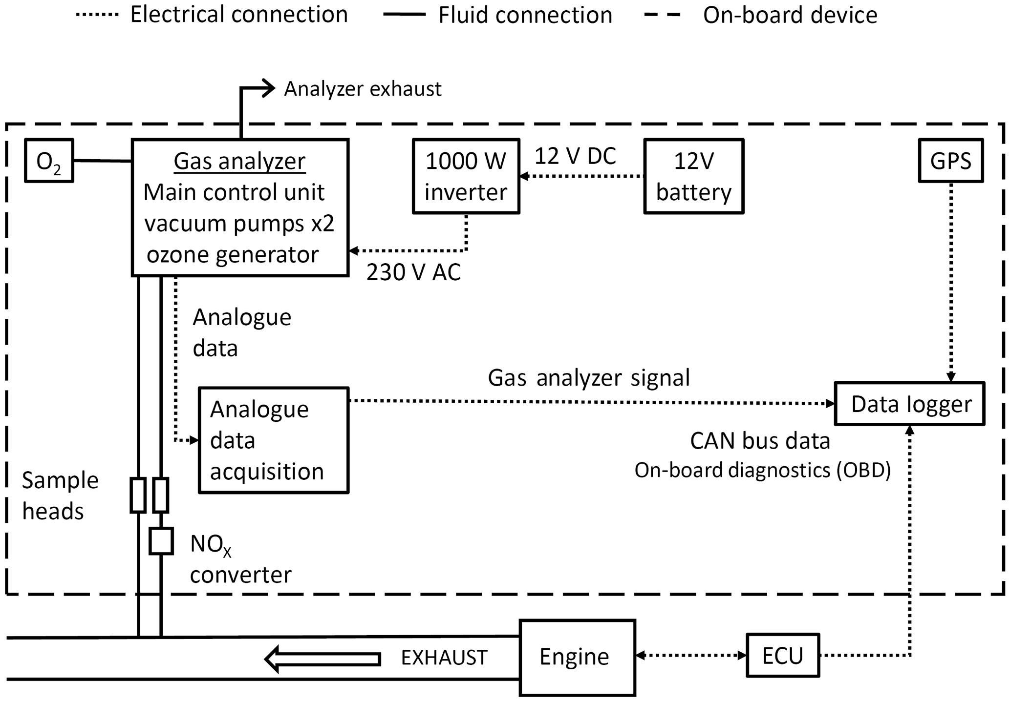
Figure 1Schematic showing the layout of the various components required for the on-board fast gas analyzer measurements. Dashed lines represent electrical connections, and fluid connections are represented by solid lines.
The methodology outlined in this paper is generally applicable to any vehicle with reasonable access to the exhaust system. This paper contains minimal discussion about the engine and aftertreatment causes of these emissions to keep the focus on the technique and the instrumentation. The case studies discussed herein are reliant on data obtained using a single two-channel analyzer operated in a configuration described below and demonstrates some, but not all, potential features of interest when using such a technique.
Figure 1 is a schematic showing the layout of the various components. A GPS module is fixed to the roof of the car, and connected to the logging computer using USB. GPS data points are subject to the standard errors inherent to GPS (Bajaj et al., 2002). These errors include but are not limited to atmospheric water vapour causing propagation delays in the radio signal and multipath errors where the signal reflects off nearby buildings, confusing the receiver. Dilution of precision due to the unfavourable positioning of satellites is also a possible source of error, meaning it can be very difficult to quantify the inaccuracy of any measurements taken. At any time the accuracy of the GPS measurement could be between 2.5 and 10 m circular error probable (CEP). However, GPS is a precise measurement technique with finest achievable resolution of 11 cm at 52∘ N. GPS is logged at 10 Hz, though this was set to 1 Hz for the London drive cycle due to this being an initial test of the technique. The 100 Hz emissions data was provided by a two-channel fast-response chemiluminescence analyzer (Reavell et al., 1997), situated in the rear of the vehicle cabin, powered via an inverter from a large capacity 12 V battery so as to avoid unnecessarily loading the engine. The analyzer data was binned according to GPS midpoint such that on average the mean of 10 analyzer concentration values are mapped onto a single GPS point, resulting in a high precision spatio-temporal emissions measurement (rather than just one concentration measurement per spatial point). The analyzer was reconfigured from its standard laboratory layout to minimize its size and power consumption, making it suitable for on-board use. Engine data was logged from the vehicle's on-board diagnostics (OBD) port, which enables access to the controller area network (CAN) data from the ECU. These data are available at a maximum rate of 10 Hz.
The 1100 mAh, 12 V battery, and 1000 W inverter supplied power to the gas analyzer for > 120 min. Not shown in the schematic are two video cameras with audio recording: one aimed at the gear selector and another aimed forwards through the front windscreen. The video cameras record to internal SD cards which are later time-aligned to the fast on-board measurement data.
The analyzers were tested for vibration signal insensitivity by logging the output to calibration gas while subjecting the rear of the vehicle to shock vibrations whilst stationary. All data are logged to one computer running a custom data acquisition program written in LabVIEW 2015. The data acquisition system merges the analogue, CAN, and GPS data on a common time-base for ease of processing (logged at 10 Hz). The program also outputs a spatially resolved dataset where each data point corresponds to a physical location with all faster data averaged between each time step.
Regarding sampling location, the gasoline emissions data recorded for this study was taken from an emissions development vehicle which was being used to establish direct links between engine operating parameters and tailpipe emissions; a sampling pipe fitted through the vehicle floor to two sampling points, one before the three-way catalyst and one post catalyst but pre-muffler. For engine calibration applications, having pre and post-catalyst sampling is essential to understanding aftertreatment operation and excellent time alignment. For air quality applications, analyzing post-catalyst data is more beneficial. The diesel data was taken from a vehicle for which floor drilling was not favoured and therefore the tailpipe data was taken post-muffler. The effect of the diesel vehicle's muffler on the measured ppm signal yielded a delay of approximately 0.4 s equivalent to an artificially early appearance of emissions of about 3 m distance in the pollutant deposition positioning at 30 km h−1 vehicle speed. This could be corrected for by post-processing if desired. For air quality interpretation alone, tailpipe measurements are adequate, but pre-catalyst measurements are required to correlate engine and driver inputs more accurately to these emissions.

Figure 2Overview maps showing NOx emissions from the diesel and gasoline vehicles driven around London (a) and Cambridge (b). Tailpipe emissions higher than 1 g km−1 per GPS point are circles coloured in black. Points of interest are numbered: (1) traffic light, (2) motorway ramp, (3) speed bumps (Map tiles by Stamen Design, under CC BY 3.0. Data by OpenStreetMap, under ODbL.).
2.1 Diesel-fuelled vehicle
Diesel emissions were measured from a Euro 5 compliant, 2.0 L, diesel passenger car with 96 000 km of operation, fuelled with standard UK pump diesel fuel (European Standard EN 590:2013, 2013). The vehicle was in good repair and in current use with no form of NOx aftertreatment (e.g. a catalytic convertor). For fleet context, diesel vehicles classified Euro 5 and earlier account for approximately 87 % of the UK's licensed diesel cars in 2016 (DVLA, 2017). One channel of the analyzer was configured for measurement of [NO] and the other for measurement of [NO] + [NO2] = [NOx] via an NO2 converter (which decomposes NO2 to NO). The sampling pipes from these two channels were connected to a single stainless-steel sample pipe entering the vehicle's tailpipe, penetrating 200 mm inside the rear muffler. The resulting response time of this sampling arrangement was approximately 20 ms, but engine exhaust transients are heavily damped by mixing in the muffler volume. However, depending on exhaust flow rate, transients can be seen with an observed rise time of approximately 100 ms, suggesting that an installation of this manner is suitable for this application. This sampling technique measures the tailpipe concentrations at street level (e.g. before turbulent dilution in the vehicle's wake). The emissions data was logged at 100 Hz.
The London route was chosen because it has been used by Transport for London for emissions studies in the past (unpublished), and the drive duration was 2.5 h for the 53 km of this route (shown in Fig. 2a). An urban route around Cambridge, UK passing near continuous air quality monitoring stations was also designed and used for comparison of diesel and gasoline vehicle emissions (shown in Fig. 2b).
2.2 Gasoline-fuelled vehicle
Gasoline emissions were measured with a Euro 4 compliant, 1.6 L, turbocharged GDI passenger car with 80 000 km of operation, fuelled with standard UK pump unleaded gasoline fuel (European Standard EN 590:2013, 2013). The vehicle was in good repair and in current use. For fleet context, gasoline vehicles classified Euro 4 and earlier account for approximately 66 % of the UK's licensed gasoline cars in 2016 (DVLA, 2017).
The sampling points on the gasoline vehicle were different from the diesel vehicle as it was anticipated that the NO2 emissions would be relatively low (NO2 being mainly a byproduct of diesel-powered internal combustion engines) (Heywood, 1988). The first channel of the fast CLA was fitted upstream of the three-way catalyst in the exhaust (hereafter referred to as “engine-out”) and the second channel was fitted downstream of the three-way catalyst (upstream of the muffler, hereafter referred to as “tailpipe”).
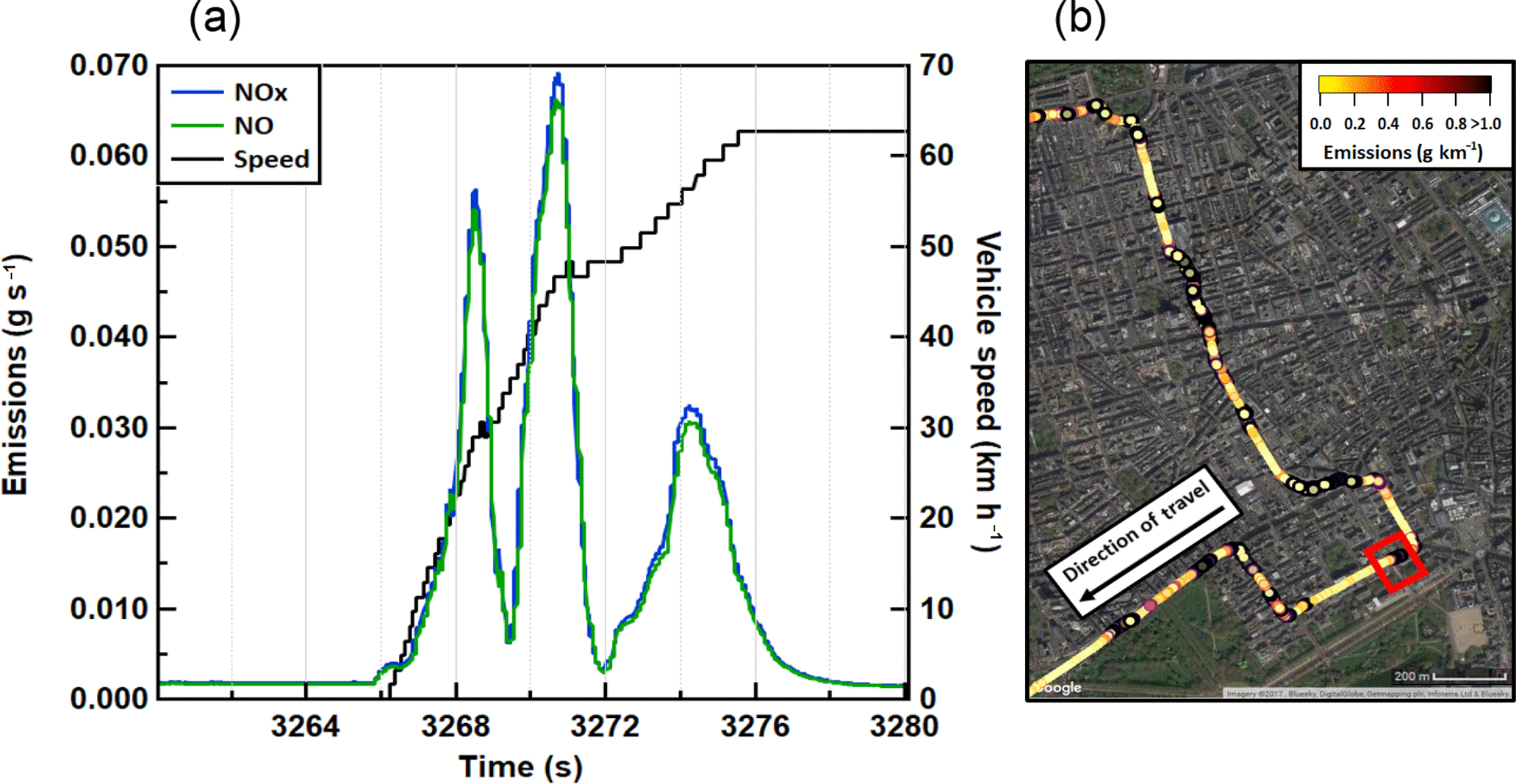
Figure 3Time series of NOx, NO, emissions in g s−1 of the diesel vehicle with vehicle speed of a traffic light pull-away in central London, UK. The red box represents the spatial component of the graph data, shown in the context of the city area.
The gasoline vehicle was driven around the Cambridge route and by comparing the engine-out to the tailpipe data, the conversion efficiency of the three-way catalyst could be calculated.
Continuously logged data (two-channel gas measurement, OBD data, and GPS location) when combined with exhaust mass flow (see below) result in two main data products: (1) gaseous mass emissions (e.g. NOx in g s−1), with vehicle speed and other diagnostic data, and (2) spatially binned exhaust mass emissions in g km−1. Data product (1) is essentially gas analyzer “raw data” converted into mass, and the time resolution is very high, limited only by the analogue data collection of the gas analyzers (and for vehicle speed, limited by the CAN-bus). Data product (2) is limited by the GPS acquisition speed (e.g. 10 Hz), and the emissions data are binned according to GPS midpoints. In binning the data, the mean values between each GPS bin midpoint are calculated, resulting in an average mass emission across the GPS point.
Mass air flow (MAF) data have been used when available from the ECU (i.e. the diesel Euro 5 vehicle), and where MAF data are not available from the ECU it has been calculated using intake air temperature, engine speed, manifold pressure, the dimensions of the engine, air ∕ fuel ratio, and an estimation of volumetric efficiency based on empirical calculations (i.e. the gasoline Euro 4 vehicle).
Since September 2017, EU vehicle emissions legislation requires new vehicles to comply with RDE requirements (EU Commission, Article 2016/427, 2016) in an attempt to make vehicles less polluting over an extended (and largely unpredictable) set of operating conditions compared with the standard drive cycles which have been used to date (United Nations, 2013). One of the main challenges in capturing the more dynamic conditions of RDE is the harsh transient driving behaviour for which fast response emissions analyzers are well suited. For the purposes of illustrating the applicability of this technique, the results have been broken up into several representative aspects of real world driving, highlighting areas of interest shown in Fig. 2 that require fast measurement to capture transient phenomena: (1) traffic lights, (2) motorway ramps, and (3) speed bumps.
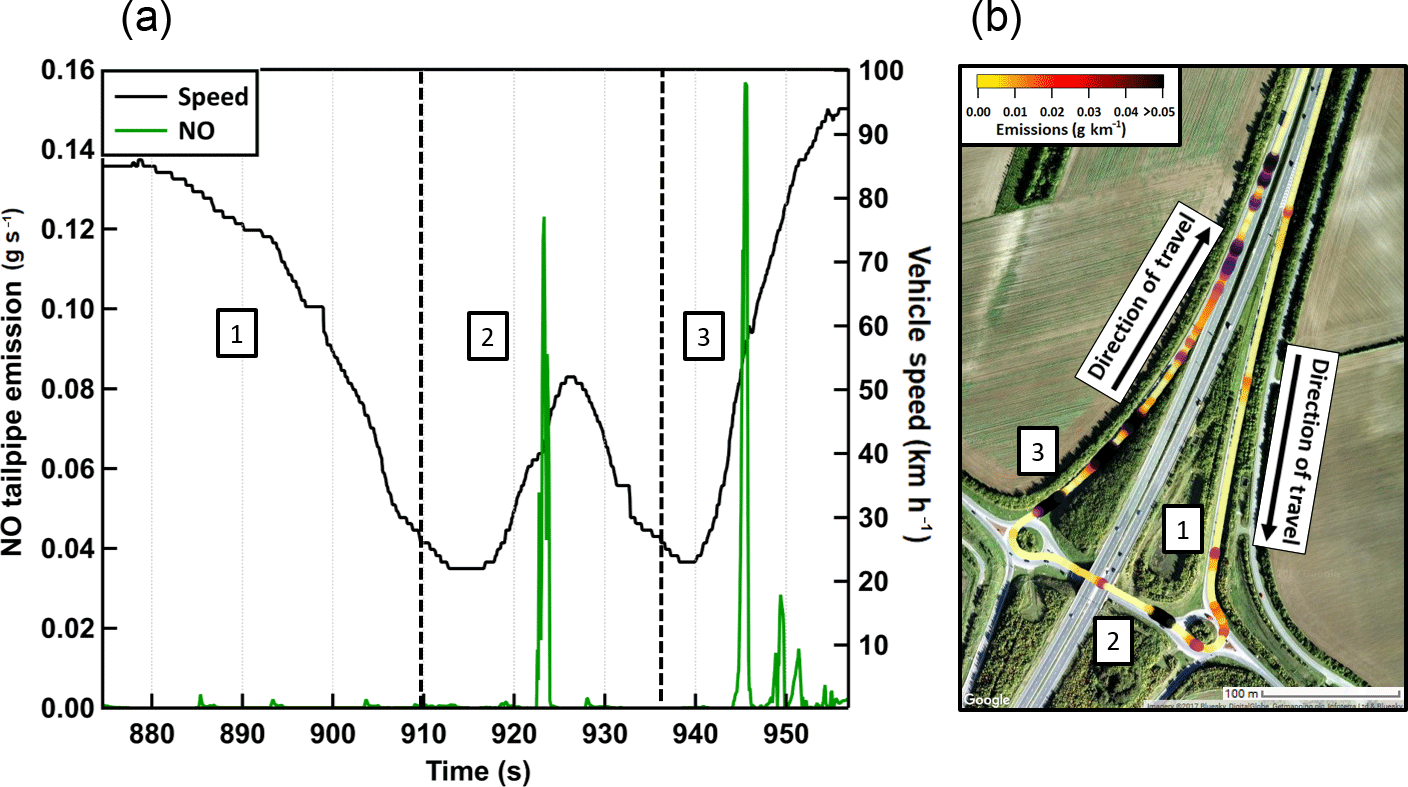
Figure 4Emissions measurements associated with coming off, traversing, and rejoining a motorway shown in three sections; (1) exiting the motorway, (2) crossing under the motorway, and (3) rejoining the motorway. Panel (a) shows the fast NO emissions (g s−1) with vehicle speed on the right axis, and panel (b) shows the route of the vehicle, coloured by NO emissions in g km−1. Note the different units on the scales for each plot, and that values over 0.05 g km−1 are all coloured black in order give sufficient dynamic range on the colour scale.
3.1 Traffic lights
Figure 3 shows the diesel NOx emissions increasing from a 2.0 ± 0.8 mg s−1 baseline when stationary, associated with sustained lean operation of the engine during the idle period, to around 70 ± 6 mg s−1 during the accelerative phases (increased engine load) following each gear change after pulling away from the traffic lights. The NOx emissions increase slightly after vehicle speed increases (i.e. accelerates) at around 3266 s due to gaseous mixing and gas transit time in the exhaust of the vehicle. This would be avoided by sampling upstream of the muffler, where sampling port installation, not desirable on all vehicles, is required. Figure 3b is a satellite view of central London, with NOx emissions in g km−1 shown as a function of colour of the mean value binned per GPS mid-point, for the route driven (driving direction indicated). The section of the drive shown in panel (a) is contained within the red box.
3.2 Motorway ramps
Figure 4 shows the data collected on the exit and entry slip road to a 70 mph (∼ 112 km h−1) dual-carriageway. In panel (a), a time series plot shows NO emissions from the Euro 4 gasoline engine alongside vehicle speed. Phase 1 of the manoeuvre shows the deceleration off the dual-carriageway on approach to the first roundabout. As expected when slowing down, load on the engine is very low, and emissions are therefore minimal. Phase 2 shows the navigation of the first roundabout followed by an acceleration and gear-change between the two roundabouts. Immediately after the gear change, a very short duration spike of NO can be seen at 923 s. The magnitude of this spike is in excess of 120 ± 36 mg s−1 – a considerable emissions peak (for reference, the current emissions standards – Euro 6 at time of publication – are 60 mg km−1 NOx for gasoline and 80 mg km−1 diesel). Using much slower conventional PEMS equipment ( ∼ 1 s), this highly time-resolved event would be significantly delayed, and smoothed out over a longer period. The true magnitude of this event would also be missed due to its short duration and its spatial location would be difficult to place. The inclusion of simultaneous GPS data identifies such emissions hot spots spatially. The scale of the spatial markers on Fig. 4 correlate colour to the mean NO emissions at that time and location (i.e. values over 50 mg kg−1 are coloured the same as at 50 mg kg−1). A black data point can be seen on the exit of the first roundabout to show the emissions at 923 s. A further spike in emissions was observed at the second roundabout due to a second deceleration, followed by an acceleration. Phase 3 shows NO emissions spikes correlating with gear changes and high load acceleration as the vehicle joins the main dual-carriageway. The increased NO emissions with each high load acceleration following each gear change are easily visualised on the GPS map plot in Fig. 4b.
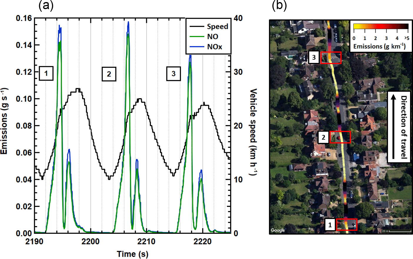
Figure 5Panel (a) NOx and NO emissions in g s−1 with vehicle speed, showing the transient behaviour associated with driving over three speed bumps in immediate succession. Panel (b) shows the geolocation of each speed bump (shown in a red box) with a coloured GPS trace showing emissions in g km−1.
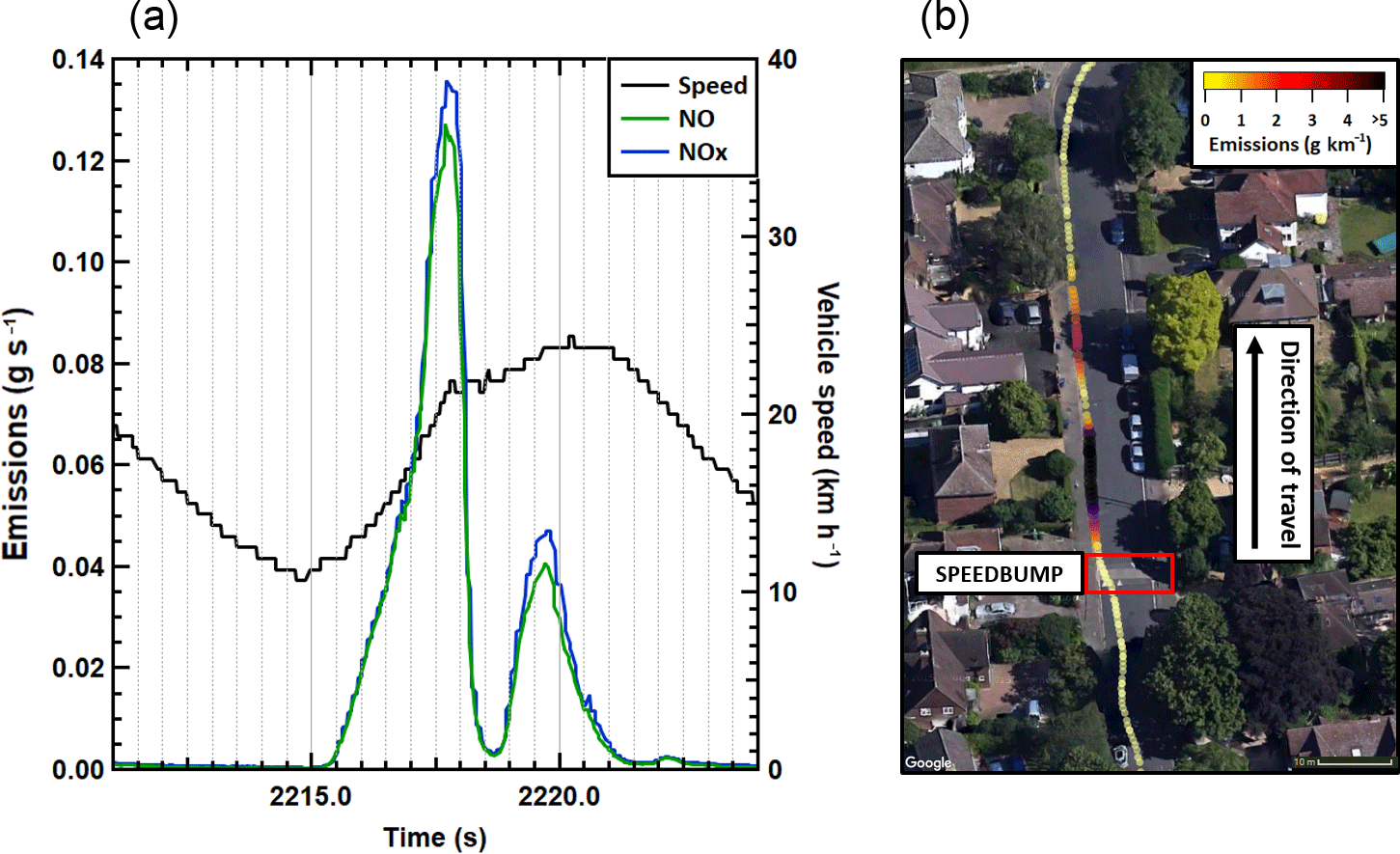
Figure 6Panel (a) NOx and NO emissions in g s−1 with vehicle speed, showing the transient behaviour associated with driving over a single speed bump in detail. The geolocation plot in panel (b) shows the emissions in g km−1 associated with the vehicle's negotiation of the speed bump.
3.3 Speed bumps
The data from the diesel vehicle most clearly shows the location of speed bumps, due to the significantly higher NOx emissions associated with all accelerative phases (i.e. higher signal compared with gasoline measurements for the same test).
Figure 5 shows NOx and NO emissions and vehicle speed against time, with a spatial plot of NOx emissions in mg kg−1 in panel (b). The NOx and NO emissions vary with vehicle speed over three subsequent speed bumps, labelled numerically on both the time-series and spatial plots. The nature of speed bumps is to force the driver to slow significantly before accelerating back up to cruising speed, and are often located immediately outside schools or in residential areas as a safety measure. The largest emissions are again associated with the acceleration which occurs immediately following each speed bump, as the driver tends to accelerate towards the speed limit. The acceleration is briefly interrupted by a gear change which is easily identified by the significant reduction in NOx emissions followed by an immediate sharp increase. The fast response time of this setup illustrates the high temporal resolution of each of these fast transient features. Figure 6 shows the characteristics associated with a single speed bump. Where decelerations are fairly sharp and fuel shut-off occurs, a sharp drop in NOx is observed as there is no combustion producing NOx emissions. Further, the drop in emissions at 2218 s is due to a gear change. The inclusion of traffic calming measures such as speed bumps outside schools may reduce average vehicle road speeds, but appears to increase local pollution significantly.
3.4 Error Propagation
An error propagation has been conducted for the data taken, using the general propagation of errors formula (Ku, 1966), based on known uncertainties for the gas analyzer, and for the diesel, data-sheet values for the on-board mass flow meter and assumed values for λ (air–fuel ratio) . This yielded values of ±5.8 % at the maximum point and approximately ±100 % for the baseline. For the gasoline, a comparison was made to a Bosch flow metre of known uncertainty and errors calculated from this, with data-sheet values for λ in this case. This yielded values of ±25.6 % at the maximum point and approximately ±140 % for the baseline. Uncertainties have been provided for all stated values.
Ultra-fast response engine exhaust emissions analyzers have been adapted for on-board vehicle use, and when combined with OBD and GPS data allow, for the first time, numerous transient features associated with the on-road driving of internal combustion engines to be examined in detail. On-board, the analyzer's sampling rate of 100 Hz captures emissions transients that would otherwise be lost or smeared when using conventional PEMS equipment or other slower analyzers. The ultra-fast analyzers therefore present a time resolution improvement of two orders of magnitude over PEMS. In addition, PEMS GPS data are recorded at 1 Hz, whereas the location data in this study is logged at 10 Hz. This realises a 10× spatial resolution benefit in the logged location data and a 100× analyzer response time benefit, which matches the resolution of the GPS. The contribution of these aspects will give a vast spatio-temporal improvement.
For an application such as the identification of pollution “hot-spots” for the improvement of urban air quality, it is important to understand any road features which promote transient accelerator pedal input on a local scale, and therefore using a measurement technique able to sample many points throughout a short duration transient is fundamental to understanding its causes.
The analyzers were adapted for on-board use by reducing their size and power requirements far below the original laboratory specification thereby allowing for at least a 2 h operating interval. Further, OBD and GPS data were logged simultaneously with exhaust emissions such that the aforementioned transient features can be analyzed with a high temporal resolution and with precise location. Using exhaust mass flow (or a derived value), NOx concentrations were converted to g s−1, and then binned into the simultaneously logged GPS points as g km−1, resulting in a spatio-temporal data product that can be overlaid onto satellite mapping services (e.g. Google Maps, OpenStreetMap) for the easy identification of emissions hot-spots. A selection of hot-spots was explored in the data analysis, giving insight into the transient features associated with the high emissions at these locations. Traffic lights, motorway ramps, and speed bumps were three examples of daily driving conditions that benefit from fast-gas measurement in terms of identifying under what engine conditions spikes in emissions occur, and the resultant emissions hot spots in terms of geographic location. Namely, the accelerations (including their gear changes) caused by traffic conditions and road layout are the cause of these high emissions. NOx was chosen for this study as being one of the main urban air quality pollutants of concern, but fast response THC, CO and CO2 analyzers can also be used in a similar manner.
Further Work
Further improvements have already been made to the spatial accuracy of the positioning data. Real-time kinematic (RTK) GPS has been successfully implemented allowing an accuracy of < 1 cm to be achieved in favourable conditions, with an increased 15 Hz logging frequency. This has further increased the benefit of the spatial emissions positioning of this technique.
This paper discusses the specific technique required to take high spatio-temporal emissions data but consideration of the implications of such data is important. GPS plots of emissions hot spots could provide important information for local air quality councils and transport planning authorities. However due to the relative set-up times of such testing it is unlikely to be a useful tool for in-service compliance checks. If used correctly, emissions maps could provide recommendations on changes to improve local air quality. The most obvious change, from a purely scientific point of view, would be the removal of all speed bumps as these cause transients that contribute significantly to high NOx levels. Their placement close to schools or pedestrian areas reinforces this argument due to the direct impact on local air quality. However, such a change would have other political and safety implications far beyond the scope of this paper. Further, improvements through synchronization of traffic lights in order to streamline traffic flows may be possible. A greater uptake in driverless or at least intelligent vehicles that could feedback to a centralised traffic control centre would aid this. Drivers could also shoulder some responsibility for emissions improvement, thus education in better driving techniques or even the inclusion of a driving quality metric into licensing tests could be beneficial. Although this study includes several tests on two differing vehicles, the data set is insufficient to allow the above hypothesis to be tested. Further work in repetition of specific road elements in different vehicles, and employing different driving styles, is needed.
Data available upon request from the corresponding author.
The authors declare that they have no conflict of interest.
We would like to thank Transport for London (TfL) for supplying a Central and
West London candidate route.
Edited by:
Folkert Boersma
Reviewed by: three anonymous referees
Apte, J. S., Messier, K. P., Gani, S., Brauer, M., Kirchstetter, T. W., Lunden, M. M., Marshall, J. D., Portier, C. J., Vermeulen, R. C., and Hamburg, S. P.: High-Resolution Air Pollution Mapping with Google Street View Cars: Exploiting Big Data, Environ. Sci. Technol., 51, 6999–7008, https://doi.org/10.1021/acs.est.7b00891, 2017. a
Bajaj, R., Ranaweera, S., and Agrawal, D.: GPS: location-tracking technology, Computer, 35, 92–94, https://doi.org/10.1109/MC.2002.993780, 2002. a
Chan, C. K. and Yao, X.: Air pollution in mega cities in China, Atmos. Environ., 42, 1–42, https://doi.org/10.1016/j.atmosenv.2007.09.003, 2008. a
Collings, N. and Willey, J.: Cyclically Resolved HC Emissions from a Spark Ignition Engine, SAE Technical Paper 871691, https://doi.org/10.4271/871691, 1987. a
Crombie, H., O 'rourke, D., and Robinson, S.: Air pollution: outdoor air quality and health Draft Evidence review 2 on: Traffic management and enforcement, and financial incentives and disincentives, National Institute for Health and Care Excellence, available at: https://www.nice.org.uk/guidance/ng70/documents/evidence-review-3 (last access: 10 June 2018), 2016. a
Department Of Defense, U.: Global Positioning System Standard Positioning Service, 4th edn., Department Of Defense, USA, 160 pp., available at: http://www.gps.gov/technical/ps/2008-SPS-performance-standard.pdf (last access: 10 June 2018), 2008. a
DVLA: Vehicle Licensing Statistics – Table VEH211, Department for Transport Statistics, available at: https://www.gov.uk/government/uploads/system/uploads/attachment_data/file/608164/veh0211.ods (last access: 10 June 2018), 2017. a, b
EU: Commission Regulation (EU) 2016/427 of 10 March 2016 amending Regulation (EC) No 692/2008 as regards emissions from light passenger and commercial vehicles (Euro 6), available at: https://eur-lex.europa.eu/legal-content/EN/TXT/?uri=CELEX:32016R0427 (last access: 10 June 2018), 2016. a, b, c
European Standard EN 590:2013: Automotive fuels - Diesel - Requirements and test methods, European Committee for Standardizatrion, 12 pp., available at: http://www.envirochem.hu/www.envirochem.hu/documents/EN_590_2009_hhV05.pdf (last access: 10 June 2018), 2013. a, b
Heywood, J. B.: Internal Combustion Engine Fundementals, vol. 21, McGraw-Hill Inc., ISBN: 0071004998, 1988. a
Kagawa, J.: Health effects of diesel exhaust emissions – a mixture of air pollutants of worldwide concern, Toxicology, 181–182, 349–353, https://doi.org/10.1016/S0300-483X(02)00461-4, 2002. a
Kampa, M. and Castanas, E.: Human health effects of air pollution, Environ. Pollut., 151, 362–367, https://doi.org/10.1016/j.envpol.2007.06.012, 2008. a
Khalfan, A., Andrews, G., and Li, H.: Real World Driving: Emissions in Highly Congested Traffic, SAE Technical Paper 2017-01-2388, https://doi.org/10.4271/2017-01-2388, 2017. a
Kings College London: London Air Quality Network – Annual Pollution Maps, available at: https://www.londonair.org.uk/london/asp/annualmaps.asp (last access: 10 June 2018), 2013. a
Ku, H. H.: Notes on the use of propagation of error formulas, J. Res. NBS C Eng. Inst., 70, 263–273, https://doi.org/10.6028/jres.070C.025, 1966. a
Mayer, H.: Air pollution in cities, Atmos. Environ., 33, 4029–4037, https://doi.org/10.1016/S1352-2310(99)00144-2, 1999. a
Reavell, K. S. J., Collings, N., Peckham, M., and Hands, T.: Simultaneous Fast Response NO and HC Measurements from a Spark Ignition Engine, SAE Technical Paper 971610, https://doi.org/10.4271/971610, 1997. a
Samet, J. M., Dominici, F., Curriero, F. C., Coursac, I., and Zeger, S. L.: Fine Particulate Air Pollution and Mortality in 20 U.S. Cities, 1987–1994, New Engl. J. Med., 343, 1742–1749, https://doi.org/10.1056/NEJM200012143432401, 2000. a
Schmidt, H.: Implementing RDE – current status of legislation and latest test results, FAD Conference, available at: http://www.fad-diesel.de/conference-2017?file=tl_files/FAD/PDF/Konferenzen/Konferenzbeitraege/Program 15. Conference 2017 ges.pdf, 2017. a
Secretary of State for Transport: https://www.gov.uk/government/ministers/secretary-of-state-for-transport (last access: 10 June 2018), 2016. a
United Nations: Addendum 100: Regulation No. 101, 100 pp., available at: http://www.unece.org/fileadmin/DAM/trans/main/wp29/wp29regs/2015/R101r3e.pdf (last access: 10 June 2018), 2013. a
hot spots. In particular, NOx pollution was assessed in detail for a number of road network features (e.g. speed bumps).