the Creative Commons Attribution 4.0 License.
the Creative Commons Attribution 4.0 License.
 | 27 Jun 2018
Quality assessment of the Ozone_cci Climate Research Data Package (release 2017) – Part 2: Ground-based validation of nadir ozone profile data products
Jean-Christopher Lambert
José Granville
Daan Hubert
Tijl Verhoelst
Steven Compernolle
Barry Latter
Brian Kerridge
Richard Siddans
Anne Boynard
Juliette Hadji-Lazaro
Cathy Clerbaux
Catherine Wespes
Daniel R. Hurtmans
Pierre-François Coheur
Jacob C. A. van Peet
Ronald J van der A
Katerina Garane
Maria Elissavet Koukouli
Dimitris S. Balis
Andy Delcloo
Rigel Kivi
Réné Stübi
Sophie Godin-Beekmann
Michel Van Roozendael
Claus Zehner
Atmospheric ozone plays a key role in air quality and the radiation budget of the Earth, both directly and through its chemical influence on other trace gases. Assessments of the atmospheric ozone distribution and associated climate change therefore demand accurate vertically resolved ozone observations with both stratospheric and tropospheric sensitivity, on both global and regional scales, and both in the long term and at shorter timescales. Such observations have been acquired by two series of European nadir-viewing ozone profilers, namely the scattered-light UV–visible spectrometers of the GOME family, launched regularly since 1995 (GOME, SCIAMACHY, OMI, GOME-2A/B, TROPOMI, and the upcoming Sentinel-5 series), and the thermal infrared emission sounders of the IASI type, launched regularly since 2006 (IASI on Metop platforms and the upcoming IASI-NG on Metop-SG). In particular, several Level-2 retrieved, Level-3 monthly gridded, and Level-4 assimilated nadir ozone profile data products have been improved and harmonized in the context of the ozone project of the European Space Agency's Climate Change Initiative (ESA Ozone_cci). To verify their fitness for purpose, these ozone datasets must undergo a comprehensive quality assessment (QA), including (a) detailed identification of their geographical, vertical, and temporal domains of validity; (b) quantification of their potential bias, noise, and drift and their dependences on major influence quantities; and (c) assessment of the mutual consistency of data from different sounders. For this purpose we have applied to the Ozone_cci Climate Research Data Package (CRDP) released in 2017 the versatile QA and validation system Multi-TASTE, which has been developed in the context of several heritage projects (ESA's Multi-TASTE, EUMETSAT's O3M-SAF, and the European Commission's FP6 GEOmon and FP7 QA4ECV). This work, as the second in a series of four Ozone_cci validation papers, reports for the first time on data content studies, information content studies and ground-based validation for both the GOME- and IASI-type climate data records combined. The ground-based reference measurements have been provided by the Network for the Detection of Atmospheric Composition Change (NDACC), NASA's Southern Hemisphere Additional Ozonesonde programme (SHADOZ), and other ozonesonde and lidar stations contributing to the World Meteorological Organisation's Global Atmosphere Watch (WMO GAW). The nadir ozone profile CRDP quality assessment reveals that all nadir ozone profile products under study fulfil the GCOS user requirements in terms of observation frequency and horizontal and vertical resolution. Yet all L2 observations also show sensitivity outliers in the UTLS and are strongly correlated vertically due to substantial averaging kernel fluctuations that extend far beyond the kernel's 15 km FWHM. The CRDP typically does not comply with the GCOS user requirements in terms of total uncertainty and decadal drift, except for the UV–visible L4 dataset. The drift values of the L2 GOME and OMI, the L3 IASI, and the L4 assimilated products are found to be overall insignificant, however, and applying appropriate altitude-dependent bias and drift corrections make the data fit for climate and atmospheric composition monitoring and modelling purposes. Dependence of the Ozone_cci data quality on major influence quantities – resulting in data screening suggestions to users – and perspectives for the Copernicus Sentinel missions are additionally discussed.
- Article
(17446 KB) - Companion paper
- BibTeX
- EndNote


Climate studies related to atmospheric composition and the Earth's radiation budget require accurate monitoring of the horizontal and vertical distribution of ozone on the global scale and in the long term (WMO, 2010). Atmospheric ozone concentration profiles have been retrieved from solar backscatter ultraviolet radiation measurements by nadir-viewing satellite spectrometers since the 1960s, starting with the USSR Kosmos missions in 1964–1965 (Iozenas et al., 1969) and NASA's Orbiting Geophysical Observatory in 1967–1969 (Anderson et al., 1969) and Backscatter Ultraviolet (BUV) instrument on Nimbus 4 in 1970–1975 (Heath et al., 1973), and continuing with the Solar BUV(2) series after 1978 (Heath et al., 1975), the Global Ozone Monitoring Experiment (GOME) family of sensors since 1995 (Burrows et al., 1999), and the Ozone Mapping Profiler Suite (OMPS-nadir) series started in 2011 (Flynn et al., 2006). Thermal infrared (TIR) emission measurements of the ozone profile by nadir-viewing satellite spectrometers were introduced more recently with the Aura Tropospheric Emission Spectrometer (TES) in 2004 and the series of Metop Infrared Atmospheric Sounding Interferometers (IASI) since 2006. Over the past decades these retrievals have been frequently quality-checked and often improved in order to meet climate research user requirements like the Global Climate Observing System (GCOS) targets (WMO, 2010). Yet both the verification of retrieval algorithm updates and the validation of their outputs against fiducial reference measurements (FRM) are still essential parts of the climate monitoring process, to be performed by specialized independent groups (Donlon and Zibordi, 2014; Loew et al., 2017).
The data quality assessment (QA) presented in this work (as part of a series of four papers addressing total ozone columns, nadir ozone profiles, limb ozone profiles, and tropical tropospheric ozone columns, respectively; also see Garane et al., 2018) has been performed in the context of the European Space Agency's Climate Change Initiative (ESA CCI), aiming at better using satellite data records for the monitoring of essential climate variables (ECV) (http://www.esa-ozone-cci.org/, 18 June 2018). A major goal of the Ozone_cci subproject is to produce time series of tropospheric and stratospheric ozone distributions from current and historical missions that meet the requirements for reducing the uncertainty in estimates of global radiative forcing. Yet Keppens et al. (2015), based on analysis principles discussed by Rodgers (2000), have illustrated that the comparison of nadir (ozone) profiles with FRM, although very informative on a specific data product, usually is insufficient to fully appreciate the relative quality of different retrieval products and to verify their compliance with user requirements. The present work therefore adopts the more exhaustive seven-step evaluation approach established in Keppens et al. (2015), including (1) satellite data collection and post-processing, (2) dataset content study, (3) information content study, (4) FRM data selection, (5) co-located datasets study, (6) data harmonization, and (7) comparative analyses and their dependences on physical influence quantities of relevance.
Table 1Overview of the nadir ozone profile data products generated and delivered in the Ozone_cci CRDP. The products' vertical range (with number of levels or layers between brackets) and original ozone units are added in the last two columns.
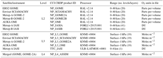
Section 2 first introduces the vertical profile retrieval schemes that have been used to generate the ESA Ozone_cci nadir profile (NP) Climate Research Data Package (CRDP). These are namely the Rutherford Appleton Laboratory (RAL, UK) version 2.14 for the backscatter UV–VIS instruments and the FORLI (Fast Optimal Retrievals on Layers for IASI) version 20151001 for the thermal infrared mission instruments, developed at the RAL and by the cooperation of the Belgian ULB (Université Libre de Bruxelles, Belgium) and the French LATMOS (Laboratoire Atmosphères, Milieux, Observations Spatiales, Paris, France), respectively. The RAL processor has been applied to retrieve L2 NP from the ERS2 GOME, Envisat SCIAMACHY, Metop-A GOME-2, Metop-B GOME-2, and AURA OMI instruments, while the FORLI algorithm has retrieved Metop-A and Metop-B IASI ozone profiles. Sections 3 to 5 then describe the validation approach and the FRM data selection, data and information content studies, and the comparative validation analyses, respectively. Section 6 concludes with general discussions of the results and with an assessment of the compliance with GCOS requirements for vertically resolved ozone climate modelling, e.g. in view of CCI contributions to the Tropospheric Ozone Assessment Report (TOAR).
2.1 CRDP overview
The 2017 release of the ESA Ozone_cci Climate Research Data Package contains 13 nadir ozone profile products in total, as listed in Table 1, and a description of their associated uncertainties. The latter are included in the comparison results discussion presented in Sect. 5. The time span of the products is indicated in Table 2. All five Level-2 (L2) backscatter UV–VIS instrument retrievals are performed by the RAL algorithm, while the infrared thermal emission measurements of the IASI instruments are processed by a collaboration between the ULB and LATMOS, using their FORLI algorithm. All instruments listed in Table 1 are on satellite vehicles with a Sun-synchronous low Earth orbit, resulting in fixed local solar overpass times (also see Sect. 3.3).
Monthly averaged Level-3 (L3) products and assimilated Level-4 (L4) atmospheric fields of the ozone profile are produced from the L2 UV–VIS data by the Royal Meteorological Institute of the Netherlands (KNMI). The L4 product is generated by assimilation of the L2 GOME and GOME-2A products (NP_GOME and NP_GOME2A). Version 0004 of the L3 and L4 products has been considered in this work (see Table 1). For the thermal infrared IASI instrument on Metop-A, only a tropospheric L3 product (prefix TTC instead of NP in Table 1) has been generated by the ULB–LATMOS team, of which the first release (version 0001) is under study in this work.
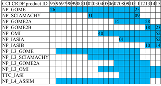
Table 2Time coverage (up to 2015) of the nadir ozone profile data products generated and delivered in the Ozone_cci CRDP (numbers indicate start and end weeks for L2 data).
2.2 L2 UV–VIS retrieval algorithm
Full time series of the ERS2 GOME (1996–2011), Envisat SCIAMACHY (2002–2011), Metop-A GOME-2 (2007–2013), Metop-B GOME-2 (2013–2015), and AURA OMI (2004–2015) nadir ozone profile data were retrieved at the RAL using version 2.14 of its RAL retrieval system. Each ozone profile is provided in volume-mixing ratio (VMR) and number density (ND) units on a fixed vertical grid with 20 levels ranging between 0 and 80 km, while the values of the 19 intermediate partial ozone column layers are provided as well. The RAL retrieval is a three-step process (Munro et al., 1998; Siddans, 2003; Miles et al., 2015).
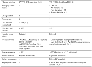
Table 3L2 nadir ozone profile filtering criteria applied in this work (first column) and their settings for the RAL UV–VIS retrieval algorithm (second column) and the FORLI TIR retrieval algorithm (third column). Values that do not comply with the settings are rejected as suggested by the respective data providers.
In the first step, the vertical profile of ozone is retrieved from Sun-normalized radiances at selected wavelengths of the ozone Hartley band, in the range 265–307 nm, which primarily contains information on stratospheric ozone. Prior ozone profiles come from the McPeters–Labow–Logan (McPeters et al., 2007) climatology, except in the troposphere where a fixed value of 1012 ozone molecules per cubic metre is assumed. A prior correlation length of 6 km is applied to construct the covariance matrix. The surface albedo, a scaling factor for the Ring effect, and the dark signal are retrieved jointly. In the second step, the surface albedo for each of the ground pixels is retrieved from the Sun-normalized radiance spectrum between 335 and 336 nm. Then, in step three, information on lower stratospheric and tropospheric ozone is added by exploiting the temperature dependence of the spectral structure in the ozone Huggins bands. The wavelength range from 323 to 334 nm is used in conjunction with ECMWF ERA-Interim meteorological fields (Dee et al., 2011). Each direct Sun spectrum is thereby fitted to a high-resolution (0.01 nm) solar reference spectrum to improve knowledge of wavelength registration and slit function width. In this step the a priori ozone profile and its error are the output of step one, except that a prior correlation length of 8 km is imposed.
RAL's radiative transfer model (RTM) is derived from GOMETRAN (Rozanov et al., 1997), but the original code has been modified substantially in order to increase its efficiency without losing accuracy. Within the RTM there is no explicit representation of clouds, but their effects are incorporated as part of the Lambertian surface albedo (from step two of the retrieval). Therefore a negative bias in retrieved ozone is to be expected where high or thick cloud is extensive and there is limited photon penetration (no “ghost column” is added). The linear error analysis of the RAL retrieval is additionally complicated by the three-step retrieval approach. Particularly as the ozone prior covariance used in step three is not identical to the solution covariance output from step one. This is handled by linearizing each step and propagating the impact of perturbations in parameters affecting the measurements through to the final solution. The estimated standard deviation of the final retrieval is taken to be the square root of the step-three solution covariance.
In this work, all nadir ozone profile screening of RAL retrievals follows the recommendations as outlined in the latest version of RAL's Ozone Profile Algorithm Product User Guide (PUG). As summarized in Table 3, the filtering requires that the normalized cost function is less than 2, the convergence flag equals 1, all ozone profile values are positive, the solar zenith angle (SZA) is below 80∘, and the effective cloud fraction (ECF) below 20 %. Additionally, for GOME-2A and B the band 1 slant column density must stay below 500 DU, and the OMI outer two pixels from each swath are rejected (see product-specific criteria in Table 3). Back-scan measurements are never considered.
2.3 L2 TIR retrieval algorithm
The Ozone_cci Metop-A and Metop-B IASI nadir ozone profile data for 2008–2015 and 2013–2015, respectively, were generated in a near-real-time mode using the FORLI-O3(Fast Optimal Retrievals on Layers for IASI Ozone) latest version 20151001 (see Hurtmans et al., 2012 for a full description of the retrieval parameters and performances). FORLI-O3relies on a fast radiative transfer and a retrieval algorithm based on the optimal estimation method (Rodgers, 2000). In the current version of FORLI-O3, look-up tables (LUTs) were precomputed to cover a larger spectral range (960–1105 cm−1) using the HITRAN 2012 spectroscopic database (Rothman et al., 2013) and correcting numerical implementation, especially with regard to the LUTs at higher altitude compared to the previous version. Ozone is retrieved using the 1025–1075 cm−1 spectral range, which is dominated by ozone absorption with only few overlapping water vapour lines and a weak absorption contribution of methanol. The a priori information used in the FORLI algorithm consists of a single global ozone prior profile. The prior variance–covariance matrix is built from the McPeters–Labow–Logan climatology (McPeters et al., 2007), as for RAL. A purely diagonal wavenumber-dependent effective noise at a value around 2 × 10⁻⁸ W cm−1 sr−1 is considered in the retrievals (Hurtmans et al., 2012).
The FORLI-O3product consists of a vertical profile retrieved on a uniform and fixed 1 km vertical grid on 40 layers from the surface up to 40 km, with an extra residual layer from 40 km to the top of the atmosphere (60 km in practice). Associated averaging kernels and relative total error profiles are provided on the same vertical grid. A posteriori filtering of the data – performed by ULB–LATMOS before data distribution – is applied to keep only the more reliable data, by removing those corresponding to poor spectral fits (root mean square of the spectral fit residual higher than 3.5 × 10⁻⁸ W cm−1 sr−1) or incomplete water vapour retrievals. Additionally, quality flags rejecting biased or sloped residuals, suspect averaging kernels, and violations of the maximum number of iterations are applied (see Table 3). Cloud-contaminated IASI scenes characterized by a fractional cloud cover above 13 % are also filtered out, as identified using cloud information from the EUMETCast operational processing (August et al., 2012). Upon discussion within the Ozone_cci community, it has been decided in this work to also reject FORLI ozone profiles whose ratios of the 0–6 km integrated column to the fully integrated column exceed 0.085. These provisional fixes, however, are corrected for in the online Ozone_cci nadir ozone profile product release.
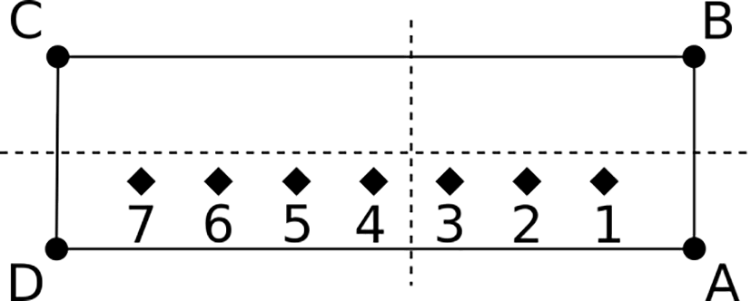
Figure 1A L2 satellite pixel ABCD is divided into subpixels (diamonds 1 to 7). Each subpixel is assigned to a L3 grid cell (indicated with the dashed boundaries) and the average and standard deviations are calculated (see text). In this example, subpixels 1–3 would be assigned to the lower-right grid cell and subpixels 4–7 would be assigned to the lower-left grid cell. The satellite pixel ABCD may have any orientation with respect to the L3 grid.
2.4 L3 monthly gridded data
For the thermal infrared IASI instrument on Metop-A, a tropospheric L3 product (prefix TTC instead of NP in Table 1) has been generated by the ULB–LATMOS team from their quality-screened L2 nadir ozone profile retrievals directly. This product consists of horizontally gridded (1∘ latitude by 1∘ longitude) monthly averages of the 0 to 6 km vertically integrated IASI-A ozone observations.
Monthly averaged L3 profile products are produced from the filtered RAL v2.14 GOME, GOME-2A, SCIAMACHY, and OMI data by the KNMI. Version 0004 of the KNMI L3 products has been used in this work (see Table 1). The KNMI L3 data consist of monthly ozone profile averages, also on a 1 × 1∘ latitude–longitude grid, containing 19 layers between 20 fixed pressure levels at each grid point. The algorithm that calculates the monthly averaged ozone fields assumes that the L2 satellite ground pixel vertices (labelled ABCD) are ordered as indicated in Fig. 1. Each pixel's across-track direction is defined by the lines AD and BC, while the along-track direction is defined by the lines AB and DC. The satellite pixel is divided into 25 subpixels, 5 in the along-track direction and 5 in the cross-track direction, and each subpixel is assigned to the L3 grid cell (the boundaries are indicated with the dashed lines in Fig. 1) containing the subpixel. The subpixel values xi are weighted by the square inverse of their uncertainties (, so the weighted mean grid cell value xc and the corresponding standard deviation σc are given by
and
respectively.
2.5 L4 data assimilation
Assimilated L4 ozone fields are produced from the screened Ozone_cci UV–VIS nadir ozone profile data by the KNMI by use of its chemical transport model TM5. The resulting L4 assimilated fields consist of 44 ozone layers (surface to 1 hPa) on a 2 × 3∘ latitude–longitude grid for four times a day (0, 6, 12, 18 h). Version 0004 of the L4 products has been used in this work, meaning that the assimilation input is limited to the L2 GOME (1 January 1996 to 31 May 2011) and GOME-2A (1 May 2007 to 30 June 2013) products (NP_GOME and NP_GOME2A in Table 1).
A complete description of KNMI's assimilation algorithm can be found in van Peet et al. (2018). The covariance matrices and the averaging kernel matrices from the L2 optimal estimation retrievals are thereby used. For the atmospheric model, the covariance matrix must be specified as well. The observations and the model data are combined using a Kalman filter technique. The averaging kernel matrix (AKM) is incorporated into the observation operator and the observation and model covariance matrices are used in the Kalman equations to calculate the analysis fields. In order to reduce biases between multiple instruments, an ozonesonde-based bias correction has been developed. For this correction, only sondes collocated with cloud-free retrievals (i.e. cloud fraction < 0.2) have been used. This correction is applied to the L2 data before the assimilation, meaning that the ozonesonde measurements involved (from 64 stations) cannot be used for the Ozone_cci L4 comparative validation exercise (see Sect. 5.6) as FRM used for comparisons have to be independent of the validated product.
3.1 Quality assessment of atmospheric satellite data
This work adopts the exhaustive seven-step satellite data QA approach presented in Keppens et al. (2015), as schematized in its Appendix A. This approach includes (1) satellite data collection and post-processing, (2) dataset content study, (3) information content study, (4) FRM data selection, (5) co-located datasets study, (6) harmonization of data representation in terms of vertical sampling and units, and (7) comparative analyses including dependences on physical influence quantities of relevance. The satellite data collection and post-processing (mainly L2 profile screening) is described by the previous section. The L2 datasets have, however, been reduced to 300 km ground station overpass datasets for the quality assessment in this work in order to reduce the total amount of data processing (i.e. satellite pixels must be within a 300 km radius from a FRM station). The FRM data selection, co-located dataset study, and data harmonization are therefore included as the successive subsections within this section. The satellite data content studies and information content studies are discussed in Sect. 4. These include statistics on the L2 station overpass data screening and spatiotemporal coverage as well as averaging-kernel-based information content measures. The comparative analysis with both spatially and temporally co-located FRM data follows later in Sect. 5.
3.2 Ground-based reference data selection
Ground-based data records from the well-established Network for the Detection of Atmospheric Composition Change (NDACC), Southern Hemisphere Additional Ozonesonde programme (SHADOZ), and other ozonesonde and lidar stations contributing to the World Meteorological Organisation's Global Atmosphere Watch (WMO GAW) networks are used as a transfer standard against which the nadir ozone profile retrievals are compared. Like for the satellite data, and prior to searching for co-locations with satellite ECV data, data screening has been applied to the FRM. The recommendations of the ground-based data providers to discard unreliable measurements are thereby followed, both on entire profiles and on individual vertical levels. Measurements with unrealistic pressure, temperature, or ozone readings are rejected automatically. Ozonesonde measurements at pressures below 5 hPa (above 30–33 km) and lidar measurements outside of the 15–47 km vertical range are rejected as well. The raw ozonesonde profiles retrieved from the public NDACC, SHADOZ data archives, and World Ozone and UV Data Centre (WOUDC) are moreover quality-screened according to the criteria outlined in Hubert et al. (2016) for a similar analysis on space-borne limb observations of atmospheric ozone: entire FRM profiles are discarded when more than half of the levels are tagged bad or when less than 30 levels are tagged good. The resulting spatiotemporal distribution of ground-based observations is summarized in Fig. 2. Despite the higher concentration of FRM in the northern mid-latitudes (20–60∘) and before 2014, the distribution is sufficiently homogeneous to consider global comparison statistics and to enable drift assessments.
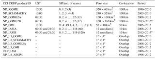
Table 4Local solar time (LST), possible scan pixel indices (SPI, with number of pixels per scan between brackets), ground pixel size, co-location distance, and temporal range of the comparative analysis. The asterisk with the Metop-B instruments indicates that the corresponding time series are not sufficiently long for drift studies. Next to the spatial co-location, a selection of the closest satellite measurement in time within 6 h for ozonesondes and 12 h for lidars takes place.
The uncertainties related to the sonde and lidar FRM used in this work are discussed in Keppens et al. (2015) and Hubert et al. (2016). Essentially, ozonesondes measure the vertical profile of ozone partial pressure with order of 10 m vertical sampling (100–150 m actual vertical resolution) from the ground up to the burst point of the balloon, usually between 30 and 33 km. Their estimated bias is smaller than 5 %, and the precision remains within the order of 3 %. Above 28 km the bias increases for all sonde types. Below the tropopause, due to lower ozone concentrations, the precision decreases slightly to 3–5 %, depending on the sonde type. The tropospheric bias also becomes larger, between 5 and 7 %. Stratospheric ozone lidar systems are sensitive from the tropopause up to about 45–50 km altitude with a vertical resolution that declines with altitude from 0.3 to 3–5 km. The estimated bias and precision are about 2 % between 20 and 35 km and increase to 10 % outside this altitude range where the signal-to-noise ratio is smaller.

Figure 2Latitude–time sampling (1996–2016) of the ground-based ozonesonde (red dots) and stratospheric ozone lidar (blue dots) measurements obtained from the NDACC, SHADOZ, and WOUDC reference network databases.
3.3 Co-location and harmonization of satellite and reference data
From all quality-approved L2 nadir ozone profile data, only those that are located within a certain radius of an NDACC, SHADOZ, or GAW ozonesonde or stratospheric lidar station location are retained for further analysis. This radius is adapted to the ground pixel size of each spaceborne instrument, in such a way that the ground-based station is roughly located within the satellite pixel (see Table 4). The possible satellite pixel index (SPI) values within each cross-track scan and the resulting number of pixels per scan are provided for each instrument in Table 4 (taking into account pixel co-adding, see Sect. 2). Additionally, only co-locations with a maximal time difference of 6 h for ozonesondes and 12 h for lidars are allowed. These time windows are chosen to generally have at least one satellite co-location with each FRM, given the satellite's fixed local solar time (LST, also see Sect. 2.1) and the fact that ozonesondes are typically launched around local noon, while lidar measurements are taken during the night. When multiple L2 satellite pixel co-locations with one unique ground-based measurement occur, only the closest satellite measurement is kept. For the L3 and L4 nadir ozone profile data, only the grid cell that overlaps with the ground-based station location is considered. All FRM within this grid cell and within the relevant month are included in the analyses for the L3 comparisons. For the 6-hourly assimilated L4 data, the unique, temporally closest, ground-based reference measurement is always less than 3 h away.
Calculating difference profiles also requires harmonization of the satellite and reference ozone profiles in terms of at least their unit representation and vertical sampling (Keppens et al., 2015). While ozonesondes report measurements in partial pressure, easily converted into VMR units and into ND using the on-board PTU measurements, the lidar data are given in ND and in general the files do not provide associated temperature profiles for a beforehand ND-to-VMR conversion. The latter has therefore been accomplished by consistently applying pressure and temperature fields that were extracted from the latest ERA-Interim reanalysis. Moreover, when there are no GPS altitude data in the ozonesonde data files, the altitude scale is reconstructed via the hydrostatic equation from the pressure and temperature recordings by the radiosonde attached to the ozonesonde. The ND profiles are integrated to partial column profiles by use of these corresponding altitude grids. The partial column profiles are then converted to the fixed satellite vertical grids by use of mass-conserved regridding, meaning that the integrated ozone column between the outer vertical edges is conserved (Langerock et al., 2015).
The optimal estimation method used in the RAL and FORLI retrieval systems consists in minimizing the difference between the measured atmospheric spectra and spectra simulated by a radiative transfer code (forward model). Since the retrieval is performed at higher vertical sampling than the actual amount of independent pieces of profile information available from the measurement, the retrieval is in general underconstrained and consequently unstable. Retrieval schemes therefore include additional constraints, e.g. in the form of a priori information on the profile, its shape, and its allowed covariance. As a result, the retrieved quantity is a mix of information contributed by the measurement and of a priori information, as represented in its vertically correlated averaging kernels. In this work, the satellite L2 and ground-based profiles' vertical smoothing is by default harmonized (i.e. reducing the vertical smoothing difference error) by smoothing of the FRM with the co-located averaging kernel (Keppens et al., 2015). The mass-conservation regridded ground-based profile xg is thereby converted into its vertically smoothed form by multiplication with the satellite profile's AKM A (in partial column units), yet taking into account the kernel's sensitivity to the prior profile xp of the optimal estimation retrieval:
The reference profile hence becomes a vertically smoothed combination of the ground-based measurement (by multiplication with A) and the prior profile (by multiplication with I − A, with I being the unit matrix of dimensions A) (Rodgers, 2000).
4.1 Data content
The nadir ozone profile CRDP L2 data content study focuses on the spatiotemporal distribution and the effect of screening of the retrieved satellite profiles in the first place, next to the regular file structure, file content, and value checks for the quantities of highest relevance (also see Table 3). Figure 3 displays the latitude–time distribution per 10∘ latitude band and per month of the percentage of screened profiles for all NP L2 station overpass (300 km) datasets (except for IASI on Metop-B). The data that are screened fail the filtering criteria suggested to data users as described in Table 3 and are therefore omitted from further analysis. Where the screening goes from 0 % (all data passes, in blue) to 100 % (no data passes, in red), one could equally insightfully interpret the plots as showing the spatiotemporal coverage of the satellite data ranging between 100 % (full coverage, in blue) and 0 % (no coverage left, in red), respectively.
The screening for the GOME and SCIAMACHY instrument retrievals is quite high (60–80 % on average), mainly due to the cloud screening that rejects all effective cloud fractions above 20 %. The lack of GOME data in the southern mid-latitudes from 2003 onwards is due to severe screening of L2 overpass data for ground stations that are all located near the South Atlantic Anomaly (SAA). The ECF has less impact on the GOME-2 and OMI instruments, but the SZA screening (if higher than 80∘) still causes meridian and seasonal coverage variations. Moreover, a latitudinal striping can be observed for all UV–VIS instrument distributions, although this is partially due to the satellite pixel co-adding before retrieval and the 300 km station overpass data selection afterwards. The decreased GOME-2B availability from June 2015 onwards points at a retrieval issue and justifies additional screening, as shown in Table 3. The IASI screening, in contrast, appears very low, but this is due to the pre-screening by the product providers before data delivery, i.e. mainly the IASI cloud screening (if the fraction is higher than 13 %) cannot be observed from the plots, but is roughly of the same order as the UV–VIS data screening. Only the seasonality of the tropospheric ozone screening (ratio of the 6 km integrated column to total integrated column > 0.085) becomes clear near the Antarctic. The IASI-B availability is fully similar to IASI-A (and overlapping in time) and therefore not shown.
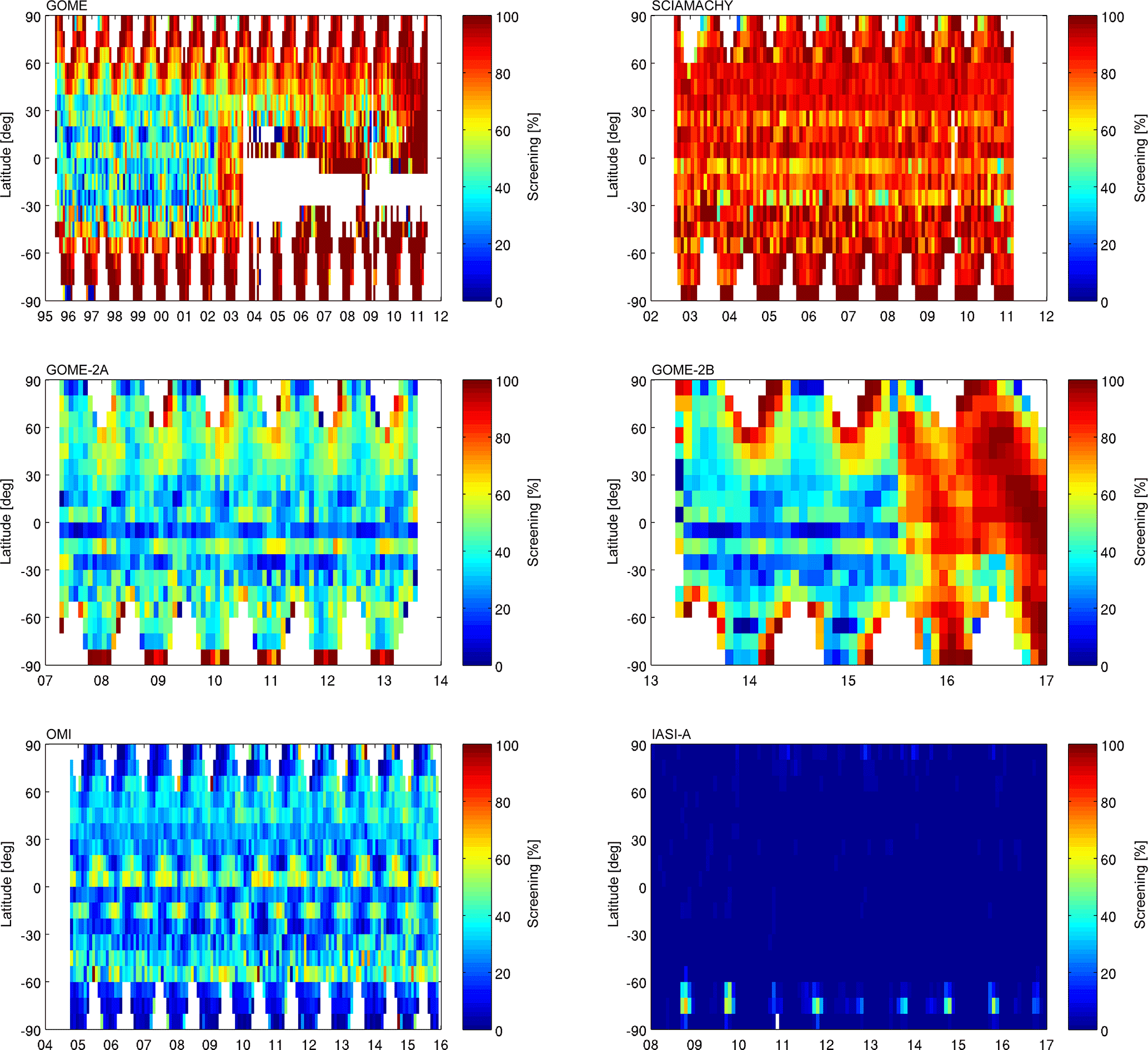
Figure 3GOME, SCIAMACHY, GOME-2A, GOME-2B, OMI, and IASI-A (left to right and top to bottom panels) latitude–time distribution of relative data screening, taking into account the quality flags presented in Table 3. The decreased GOME-2B availability from June 2015 onwards points at a retrieval issue. IASI-B is fully similar to IASI-A.
4.2 Information content
4.2.1 Information quantities
Each quantity that is retrieved using the optimal estimation technique contains information both from the satellite measurement and from the a priori profile and covariance matrix. The contribution of prior information can be significant where the measurement is weakly or even not sensitive to the atmospheric ozone profile, e.g. in case of fine-scale structures of the profile, below optically thick tropospheric clouds, and at the lower altitudes. The information distribution is captured by the retrieval's ex ante vertical AKM A, which represents the sensitivity of the retrieved state to changes in the true profile xt at a given altitude:
A study of the algebraic properties of this averaging kernel matrix, denoted information content study, can help understand how the system captures actual atmospheric signals. Through straightforward analysis, however, it can be easily demonstrated that typical information content measures as discussed in this section usually depend on the units of the averaging kernel matrices (Keppens et al., 2015). As these measures, however, should be unit-independent, fractional AKMs AF must be considered.
From Eq. (4), the fractional AKM is calculated by dividing the nominator and denominator by the corresponding retrieved and true ozone profile value, respectively. However, as the true profile is not known, it is replaced by its best available estimate [〈xt〉] being again the retrieved profile:
This approach is directly used for determining the fractional averaging kernel matrices in the UV–VIS RAL v2.14 retrieval products; therefore the RAL superscript has been added. The FORLI v20151001 algorithm that performs the thermal infrared retrievals, however, performs a unit-independent optimal estimation that immediately yields fractional AKMs. These fractional matrices are made unit-dependent by use of the prior profile before saving into the data files, allowing for more straightforward application (e.g. for vertical smoothing operations) by data users. For the information content studies presented here, this defractionalization operation therefore has to be inverted:
Hereafter, starting from the averaging kernels provided as part of the Ozone_cci CRDP L2 nadir ozone profile products, the degree of freedom in the signal (DFS) and the vertical sensitivity are studied. These quantities are given by the fractional AKM trace and row sum profile, respectively. The DFS of a retrieved atmospheric profile is a non-linear measure for the number of independent quantities that can be determined and as such loosely related to the Shannon information content (Rodgers, 2000). The vertical sensitivity to the measurement is a unit-normalized measure for how sensitive the retrieved ozone value at a certain height is to ozone values at all heights. According to Rodgers (2000, p. 47), measurement sensitivity “can be thought of as a rough measure of the fraction of the retrieval that comes from the data, rather than from the a priori”. Note, however, that the sensitivity at a specific retrieval level can nevertheless be negative or exceed unity (oversensitivity) due to kernel fluctuations and correlations between adjacent retrieval levels, as reflected in the kernel width (see below).

Figure 4GOME, SCIAMACHY, GOME-2A, GOME-2B, OMI, and IASI-A (left to right and top to bottom panels) latitude–time distribution of degrees of freedom in the signal (DFS). IASI-B is fully similar to IASI-A.
Besides the more common DFS and sensitivity information content quantities, in this work the vertical averaging kernels' offset and width are considered as well. The offset is an estimate of the uncertainty on the retrieval height registration, given either by the direct vertical distance (in kilometres) between an averaging kernel's peak sensitivity altitude zpeak and its nominal retrieval altitude znom as d(m) = zpeak(m) − znom(m) or as the so-called centroid offset dc(m) = c(m) − znom(m) (Rodgers, 2000) with
Ideally, within each kernel, this distance equals zero.
Ozone_cci user requirements also specify an upper limit of the vertical resolution of the nadir ozone profile retrievals. In the literature different methods have been proposed to estimate the vertical resolution from the width of the vertical averaging kernels (see overview in Keppens et al., 2015), but usually it is determined either as a full-width at half-maximum (FWHM) value around the kernel's peak altitude or as the Backus–Gilbert (BG) spread or resolving length around its centroid:
Whereas an averaging kernel's direct offset and FWHM width only take into account its central sensitivity peak, Eqs. (7) and (8) point out that the centroid offset and BG spread include all vertical kernel information. As a result, the centroid at a given altitude can be considered a measure of the overall retrieval barycentre for that altitude, with the BG spread showing the retrieval's full extent, also taking into account sensitivity fluctuations. Other information content diagnostics, such as the measurement quality quantifier and the AKMs' eigenvectors and eigenvalues, have previously been studied but are not reported here (Keppens et al., 2015).
4.2.2 Degrees of freedom in the signal
Figure 4 displays the latitude–time distribution per 10∘ latitude band and per month of the median DFS for all NP L2 datasets (except for IASI on Metop-B). RAL's UV–VIS DFS is typically around 5, with the lowest values for SCIAMACHY (4 to 5) and the highest for OMI (5 to 5.5), and quite stable in time, reflecting the signal degradation correction that is incorporated within the RAL v2.14 retrieval algorithm. This correction maintains the instrument's signal-to-noise ratio close to its initial level and hence reduces the effect of the instrument degradation on the retrieval's DFS. Seasonal DFS variations amount to about 0.5, which is approximately the same as the DFS decrease per decade, except for the more stable OMI retrieval. The temporal DFS behaviour is also reflected in the AKMs' eigenvalues and eigenvectors (not included). More exceptional are the two to three DFS outliers for SCIAMACHY, which typically occur in the SAA due to stratospheric intrusion of high-energetic particles (the tropospheric DFS is mostly maintained). Such SAA outliers also occur in other instrument retrievals, but to a lesser extent (also see next sections). Note that the area of missing GOME data in the tropics from 2003 due to the SAA is larger than in Fig. 3, as the DFS and other information content values are empty when all data are screened (100 % values in Fig. 3). Also note that the decreased retrieval performance for GOME-2B from June 2015 (eventually resulting in its total screening) actually has little effect on its DFS behaviour. Due to its stronger meridian and seasonal dependence, the FORLI TIR median DFS for IASI-A ranges between 2 towards the poles and 4 towards the Equator. The overall degradation, however, is negligible as for OMI. The IASI-B spatiotemporal DFS behaviour is fully similar to IASI-A (and overlapping in time) and therefore not shown.
4.2.3 Height-resolved information content
Exemplary plots containing the global GOME-2A (left column) and IASI-A (right column) information content in terms of vertical sensitivity, retrieval offset, and averaging kernel width are displayed in Fig. 5. Their dependence on DFS, SZA, or thermal contrast (TC) is introduced by the plot colour, whereby profiles corresponding to out-of-range influence quantity values are plotted in magenta. The other RAL v2.14 UV–VIS and FORLI v20151001 TIR retrieval products show similar statistics.
The vertical sensitivity profiles, which are the same in all three plots for each product, are close to unity around the ozone peak and above (25 to 45 km) for all retrieval products under consideration. Typically the sensitivity decreases above and below due to the smaller ozone concentrations (therefore the vertical range is limited to 50 km), but the actual behaviour strongly depends on the retrieval algorithm. The RAL retrieval usually results in a very strong oversensitivity around the upper troposphere and lower stratosphere (UTLS), with a median value of 3. This peak partially compensates for the undersensitivity right above and below, with the sensitivity dropping down to about 0.5 in the lowest 0–6 km column. The peak value moreover heavily correlates with the SZA, as one can expect for an UV–VIS retrieval algorithm. In contrast, some RAL sensitivity profiles quickly decrease to zero when going from 25 to 40 km altitude. These are connected to very low DFS values (around two or below), as identified to occur around the SAA. Most of the retrieval information in these profiles is therefore located around the UTLS and in the troposphere.
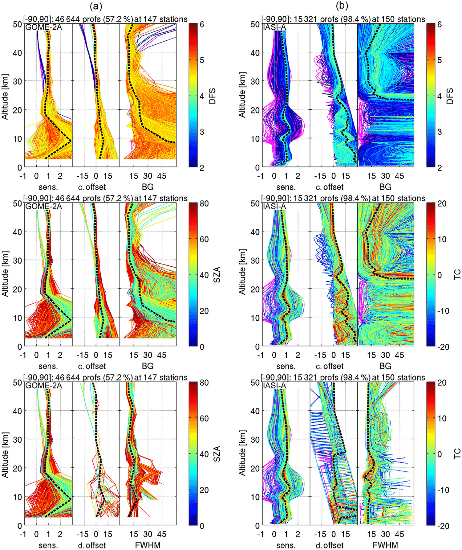
Figure 5Global GOME-2A (a) and IASI-A (b) information content in terms of vertical sensitivity, retrieval offset (in kilometres), and averaging kernel width (in km) and their dependence on DFS, SZA, or thermal contrast (TC). Black dashed lines represent median values, while out-of-range profiles are plotted in magenta. Different measures are used for the offset and kernel width in the second and third rows, which include the centroid offset (c. offset) and Backus–Gilbert spread (BG) and the direct offset (d. offset) and FWHM, respectively. Plot titles provide the absolute and relative amounts of profiles after screening and the number of ground-based overpass stations.
The IASI instrument retrievals do not show this stratospheric decline for excessively low DFS values, but instead show sensitivity outliers around the UTLS, ranging from below −1 to above 2. Although the overall IASI sensitivity variability is strongest around the Equator, these outliers typically occur in the polar regions, as can be expected from Fig. 4, and go together with excessively high retrieved ozone peaks. The strong sensitivity variability, pointing at outliers in the averaging kernel matrices, in general hampers the averaging kernel smoothing of the reference profiles before comparison (see Eq. 3), as this procedure then introduces a bias instead of reducing the vertical smoothing difference error. Usually, however, except for decreased surface-level sensitivity (0.5) and a median 1.5 peak around the UTLS with slight compensation above and below, the FORLI v20151001 sensitivity is more vertically consistent.
Also according to Fig. 5, little difference can be observed between the median UV–VIS retrieval offset in terms of its direct and centroid measures. The height registration uncertainty remains below 10 km (except again for the low DFS values), being negative in the upper stratosphere and positive towards the Earth's surface, as can be expected for any nadir ozone profile retrieval. Note, however, that the direct offset is more discrete than the BG spread due to its one-to-one connection with the vertical retrieval grid steps. This discreteness of the direct offset is even clearer for the FORLI IASI retrievals that are performed on a fixed 1 km vertical grid. The direct offset here is lower than the centroid offset on average, but amplifies some of the latter's features, like the peak and jump around 5 and 25 km altitude, respectively. The FORLI IASI height registration uncertainty in terms of the centroid offset steadily increases from zero at 40 to about 30 km near the surface, meaning that the retrieval barycentre altitude is decreasing slower than the nominal retrieval altitude. The dependence on DFS and TC, however, is rather small.
The behaviour of an averaging kernel's sensitivity and offset is typically also reflected in its width. Figure 5 demonstrates that the RAL retrieval's sensitivity peak in the UTLS goes together with a strongly increasing BG spread, exceeding 60 km towards the Earth's surface. The median FWHM width staying below 15 km indicates that the high BG-spread values are due to fluctuations in the averaging kernels of the retrieval, showing several highs and lows next to the peak value. At higher altitudes, the median BG kernel width decreases first to about 20 km, and further to 10 km in the upper stratosphere, although individual results strongly depend on the SZA. From the low up to the middle latitudes the resolving length shows little seasonal variation, but from the mid-latitudes to the polar areas an annual variation indeed appears clearly from the ground up to the lower stratosphere, with maxima in winter and minima in summer (not shown). This conduct correlates directly with the annual variation of the slant column density (highest in winter and lowest in summer).
The connection between averaging kernel offset and width is even stronger for FORLI's v20151001 TIR retrieval scheme. At 25 km and below, where the offset shows fluctuations, the BG spread is strongly variable and its median explodes, although acceptable values of the order of 15 km are found above 25 km altitude. As for the RAL retrieval scheme, the median FWHM width staying around 10 km overall indicates that the high BG-spread values are not due to the presence of a single broad sensitivity peak, but rather to strong fluctuations in the averaging kernels that are again little dependent on DFS or TC. Like already observed for the IASI vertical sensitivity, the strongest averaging kernel width variability occurs in the tropics.
5.1 Comparison statistics
The baseline output of the L2 validation exercises consists of median absolute and relative nadir ozone profile differences at individual stations or within latitude bands for the entire time series. This median difference is a robust (against outliers) estimator of the vertically dependent systematic error, i.e. the bias, of the satellite data product. The bias profiles for the entire list of stations are then combined and visualized as a function of several influence quantities in order to reveal any dependences of the systematic error. The influence quantities considered in this work are latitude (for meridian dependence), quarter (for seasonal dependence) – being December–January–February (DJF), March–April–May (MAM), June–July–August (JJA), and September–October–November (SON) – total ozone column, DFS, SZA, scan pixel index (SPI), (effective) cloud fraction (for the UV–VIS products), TC (for the TIR products), and time. The latter actually results in drift studies, i.e. the annual or decadal bias change of the satellite product with respect to the ground-based reference time series.
Besides the median difference, the Q84–Q16 or 68 % interpercentile spread (IP68) on the differences is also calculated as a robust estimator of the random errors in the satellite data product, i.e. the precision profile. However, this spread on the differences will also include contributions from ground-based random uncertainties (limited to a few percent, as indicated in Sect. 3.2) and representativeness (sampling and smoothing) differences between the satellite and reference measurements, and therefore in fact provides an upper limit on the actual satellite uncertainty. In case of a normal distribution of the ozone differences, median and IP68 are equivalent to mean and standard deviation, but they offer the advantage to be much less sensitive to occasional outliers.
The long-term stability of the systematic errors in the ozone data products is a key user requirement. Robust linear regressions including an uncertainty estimate based on a bootstrapping approach (Hubert et al., 2016) are performed on the satellite–ground difference profiles for all stations within the predefined latitude bands or on the global scale. The uncertainty on the global drift that is as such introduced by inhomogeneities across the ground-based network is of the order of about 5 % decade−1, but in fact partially covered by the confidence interval obtained by the bootstrapping. This value was estimated from the standard deviation on the ensemble of single-station drift estimates in ground-based comparisons with limb-sounding instruments by Hubert et al. (2016), who use the same quality-checked selection of FRM stations. To avoid spurious effects due to a seasonal cycle in the differences, only time series of 5 years or longer are used for this drift assessment. Therefore Metop-B GOME-2 and IASI instruments are excluded from the drift studies (indicated with an asterisk in Table 4). Moreover, only fully available years of the satellite datasets have been considered for comparative analysis in order not to introduce seasonal effects at the beginning and the end of each time series.
Due to the availability of assimilated global ozone fields every 6 h, the L4 comparative validation approach is fully similar to the L2 statistics described above. The strongly reduced amount of parameters in the L4 data product files, however, reduces the number of influence quantity dependences that can be studied. These have therefore been limited to the latitude, quarter, and time (drift). Next to that, as vertical averaging kernel matrixes are only available for the L2 retrieved data, no averaging kernel smoothing can be applied before comparison. Yet as mentioned in Sect. 2.5, the L2 averaging kernel matrices are incorporated into the equations to calculate the analysis fields. Also remember that the satellite instrument bias correction by use of ozonesonde measurements, the 64 stations involved are not used for the L4 comparative validation exercise.
The situation is quite different for the validation statistics of the L3 monthly gridded averages. No L2 averaging kernels are used for the data generation and no merging or bias correction are implemented. The satellite-based and 1 × 1∘ gridded NP L3 data can be compared with spatially co-located ground-based reference profiles xr directly or with monthly (gridded) averages 〈xr〉 of the latter (i.e. a ground-based L3-type dataset). Yet both approaches introduce similar spatial and temporal representativeness errors into the difference statistics because taking (monthly) averages as a bias estimator 〈Δx〉 yields comparable outcomes:
For sufficiently fine-gridded L3 data, the comparisons can therefore be limited to direct differences with ground-based reference measurements, if one additionally only considers ground-based stations with a sufficient number Nm of valid measurements per month. This number has been set to six (per month, or about at least one measurement every 5 days) in the L3 validation presented in this work. As such, an implicit averaging of at least six ozonesonde or lidar measurements per month is introduced in the comparison statistics. The 1 × 1∘ box that overlaps with the ground measurements is thereby taken as the co-located measurement. Due to this high horizontal resolution of the Ozone_cci L3 satellite nadir ozone profile products and the constraint on the temporal representativeness of the ground-based data, representativeness errors are thus kept to a minimum.
5.2 L2 UV–VIS nadir ozone profiles
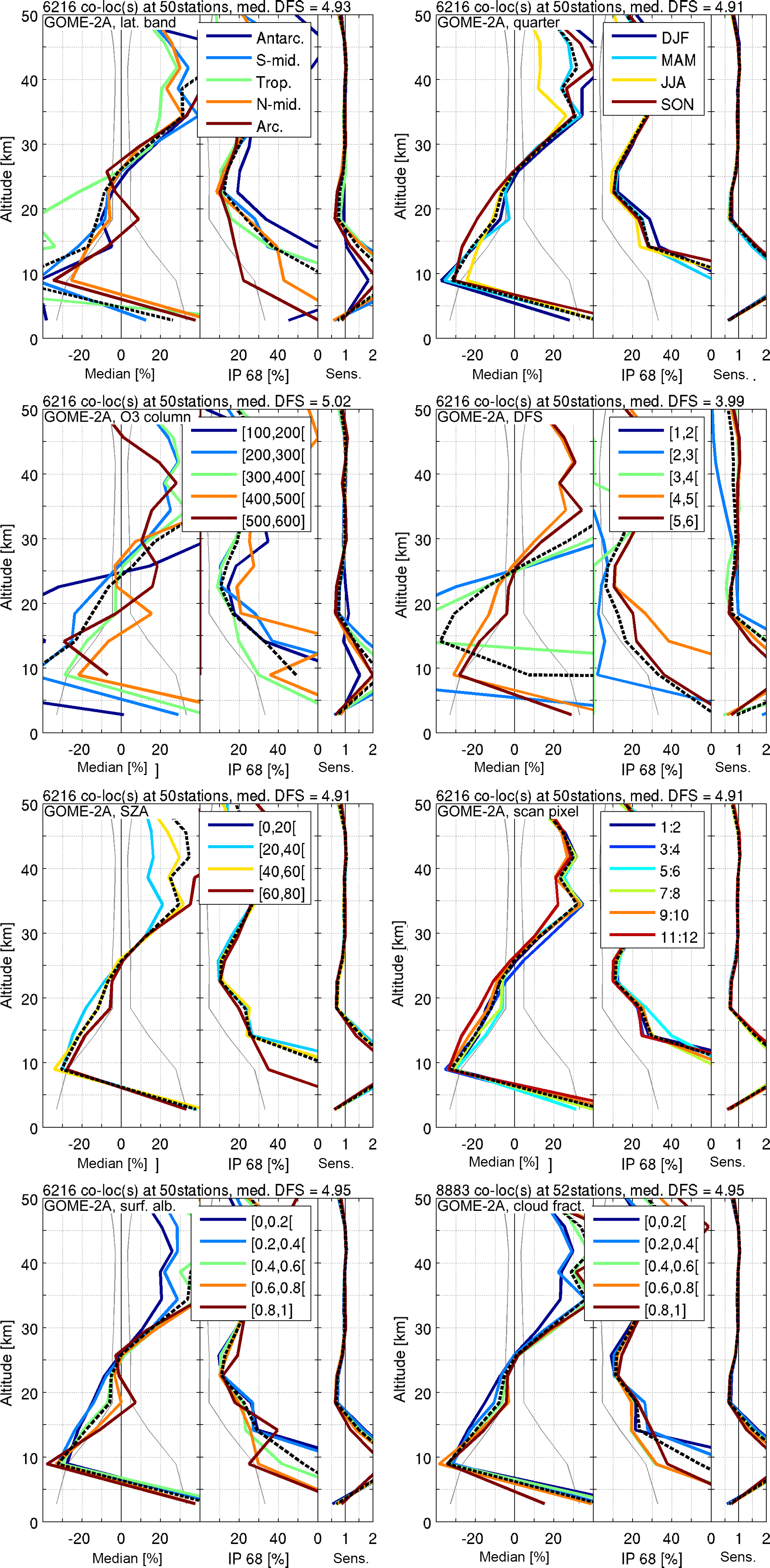
In this section comparison results between L2 RAL v2.14 nadir ozone profiles and ground-based ozonesonde and lidar measurements are reported in the form of statistics on the median relative difference (bias) and 68 % interpercentile spread of ozone differences as a function of several influence quantities. Figures 6 to 10 contain the results for GOME, SCIAMACHY, GOME-2A, GOME-2B, and OMI, respectively, as a function of latitude, quarter, total ozone column, DFS, SZA, SPI, and effective cloud fraction. Note that the number of comparisons (shown in each plot title) is higher for the latter as the ECF filter has been switched off. Estimates of the relative satellite errors provided with the RAL v2.14 products have been added to the graphs (grey lines) in order to discuss them with respect to the ozone differences and spreads. In each plot the third subgraph displays the median sensitivity of the retrieved ozone profile as a function of altitude (and the relevant influence quantity), as calculated from the fractional RAL v2.14 vertical averaging kernels.
Before discussing the comparison results in terms of influence quantities, it is interesting to note that the vertical smoothing of the ground-based reference data with averaging kernels mostly yields qualitatively similar bias and spread estimates as when merely the regridded data are considered (not included). The comparisons from regridded reference data, however, show a vertically oscillating structure (as smoothing difference error) that largely disappears for the kernel smoothed comparisons. This structure is strongest around the tropics, yielding significant differences between the regridded and smoothed data, mostly due to a positive bias peek just below 20 km for the regridded data. The corresponding comparison spreads indicate that the random uncertainty on the bias is reduced by about 10 % on average by applying the averaging kernel smoothing. This value provides a rough estimate of the vertical smoothing difference error between the ground-based reference data on the one hand and the satellite data on the other hand.
Focussing on the comparisons involving averaging kernel smoothed partial column profiles, one observes that generally the five RAL v2.14 UV–VIS retrieval products agree similarly with the ground-based data, showing a rather typical Z curve with zero biases approximately at 5 and 25 km altitude (the third around 55 km is not on the plots because of the sparseness of the FRM data availability above 50 km). The negative bias peak in the UTLS and above (5 to 25 km) and the positive bias peak in the upper stratosphere (between 25 and 55 km) both amount to about 20 to 40 %. Comparison results for the 0–6 km subcolumn show that the bias again shifts towards 40 % positive values in that layer, with the exception of the OMI instrument that keeps its median tropospheric bias within 10 %. The sensitivity for this lowest layer, however, is reduced to about 0.5, meaning that generally about 50 % of the retrieval information comes from the prior profile rather than from the measurement. In the 0 to 45 km altitude range, the UV–VIS nadir ozone profile comparison uncertainties in terms of the 68 % interpercentile spread display a U-shaped curve with a minimum of about 10 % around 25 km. The uncertainty increases to roughly 40 % at 45 km, to slightly decrease again above, but rises even more strongly where the sensitivity profile peaks and towards the ground.
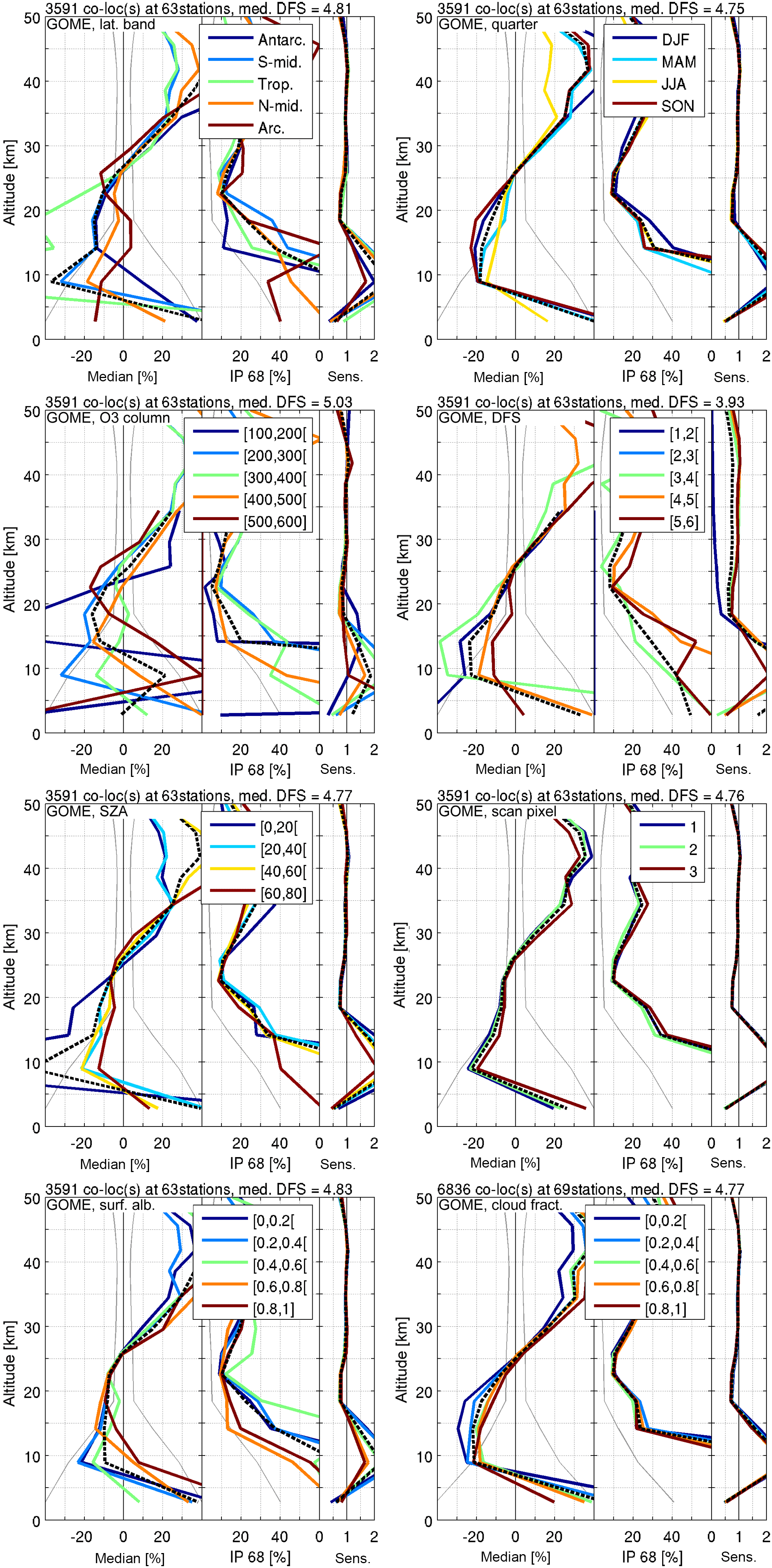
Figure 6Median relative differences, 68 % interpercentile spreads, and vertical sensitivities for comparison of RAL v2.14 L2 GOME retrieved profiles with ground-based reference measurements (1996–2010). The same difference and information statistics are redistributed in each plot over several influence quantity ranges, with the influence quantities being (from left to right and top to bottom panels) latitude, quarter, total ozone column (DU), DFS, SZA, scan pixel index, surface albedo, and effective cloud fraction. In the corresponding legend entries, open brackets are used to indicate that the last value is not included (i.e. values in the set go up to, but do not equal, the last value). The black dashed line shows the average of the coloured curves, while light grey lines indicate the satellite uncertainty provided in the product. The number of comparisons is higher for the latter as the ECF filter has been switched off.
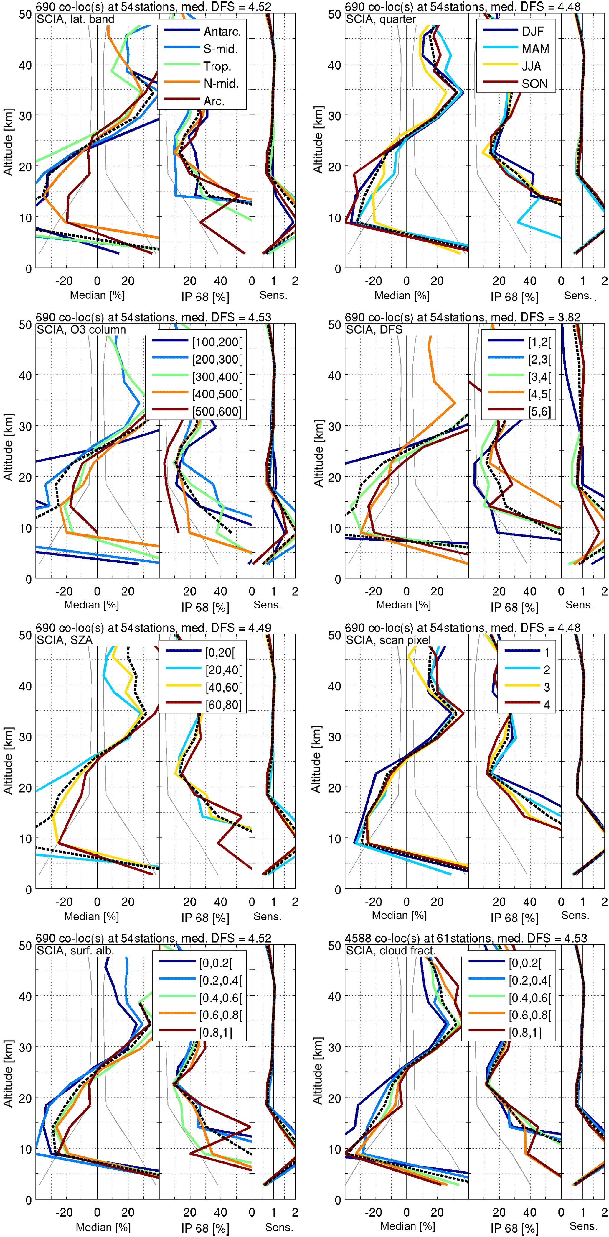


The individual L2 UV–VIS comparison graphs also contain information on the validity of ex ante uncertainties provided for the satellite nadir ozone profile retrievals (thin grey lines). The relative random error reported in the RAL v2.14 data files amounts to about 5 % at the altitude of the ozone maximum, up to about 10 % at higher altitudes, and up to 40 % in the lower troposphere. In theory the IP68 spread should be close to the combined uncertainty of the satellite data, the ground-based data, and metrology errors due to remaining differences in vertical and horizontal smoothing of atmospheric variability (including co-location mismatch errors). The latter is difficult to assess, but one can expect that the bias and spread estimates resulting from the comparisons, including AK smoothing, are close to the combined uncertainty of satellite and ground-based data, or at least the ex ante satellite uncertainty in practice (Miles et al., 2015). The plots in Figs. 6 to 10 show that this is hardly the case (also see the discussion in the previous section). The satellite measurement uncertainties provided in the product files do not cover the systematic and random uncertainties obtained by FRM comparisons (subtraction of the FRM uncertainties discussed in Sect. 3.2 does not make a difference). This means that the total satellite measurement and retrieval uncertainty is typically underestimated in the RAL v2.14 nadir ozone profile products, because the ex ante uncertainty under consideration only includes random noise errors. Only for the OMI tropospheric ozone data with a bias within 10 % does the combined uncertainty come close to the ex ante uncertainty. The total ex post satellite uncertainty is an unknown number because of precision ignorance, but can be estimated to range in between the combined (quadratic sum) bias and satellite random uncertainty and the combined bias and comparison spread (although the latter contains error contributions that are not part of the satellite observation, like co-location mismatch).
Looking at the dependence of the L2 UV–VIS product comparison results on the eight influence quantities shown in Figs. 6 to 10, one can observe that the latitude band and total ozone column have the biggest impact on the RAL v2.14 retrieval performance. Especially in the UTLS and the troposphere the comparison variability is very high, which is also reflected in the strong differences in spread between different influence quantity ranges. Smaller biases are typically obtained in the Northern Hemisphere and for intermediate to larger total ozone columns. Larger ozone columns are indeed expected to result in an improved satellite measurement and retrieval sensitivity, and thus more stable averaging kernel behaviour with smaller vertical dependences. In contrast, the DFS and SZA behaviour is somewhat smaller and, as one can again expect for UV–VIS observations, rather similar, with the higher SZAs typically corresponding to the larger DFS values (mainly from the stratosphere), the largest stratospheric biases, and the smallest tropospheric biases. The latter could be due, however, to a somewhat reduced tropospheric sensitivity, bringing the retrieved profile closer to the prior profile. This effect is most clear for the GOME and SCIAMACHY instruments though, while the overall DFS dependence for the other instruments is less obvious. For all UV–VIS instruments except GOME-2B, however, some satellite profiles with very low DFS, nearly zero stratospheric sensitivity, and high bias occur (mainly in the SAA, see previous sections). These profiles result from retrievals without stratospheric measurement information (hence the low DFS) and should appropriately be screened by users accordingly, e.g. using a DFS < 3 flag. Nadir ozone profiles flagged as such should then only be considered for tropospheric ozone monitoring or fully rejected because of the increased bias.
Again more or less in line with nadir ozone profile retrieval expectations, the comparison results depend little on the surface albedo and effective cloud fraction, except for the lowermost 0 to 6 km retrieval layer. Higher ozone concentrations logically correspond with lower cloud fractions and higher albedos. Note, however, that the ECF and surface albedo dependence is also reflected, yet inversely, in the UTLS, due to the typically high sensitivity peak in this region and the low compensation above. This effect is most clearly visible for the GOME-2B and OMI instruments. Instead of the full-profile effective cloud screening suggested by the RAL team now, one could thus apply layer screening up to the UTLS instead. Finally, for the UV–VIS retrievals under consideration the quarter and scan pixel index have hardly any effect on the comparison results, meaning that the RAL v2.14 retrieval algorithm copes with ozone seasonality and instrument viewing angle effects very appropriately.
5.3 L3 UV–VIS monthly gridded ozone product
Median relative differences and 68 % interpercentile spreads for comparison of L3 GOME, SCIAMACHY, GOME-2A, and OMI data with ground-based reference measurements are presented in Fig. 11. The same difference statistics are redistributed for each instrument over two influence quantity ranges, with the influence quantities being the latitude and quarter. Note the high numbers of co-locations in the title of each plot, as for each ground-based reference measurement an overlapping L3 data grid cell can be identified. As can be expected, the median relative differences roughly follow the bias features of the respective L2 datasets for their comparison with ozonesonde and lidar data. These features, together with the corresponding spreads, seem to be enlarged due to larger differences in spatiotemporal representativeness. The latter results from the lack of averaging kernel smoothing that reduces vertical smoothing difference errors and the limited amount of reference data measurements per month (although at least six, see previous sections). Note, however, that the lack of kernel smoothing instead reduces the L3 spread for the lowest level, which has a strongly reduced sensitivity in comparison with the levels above.
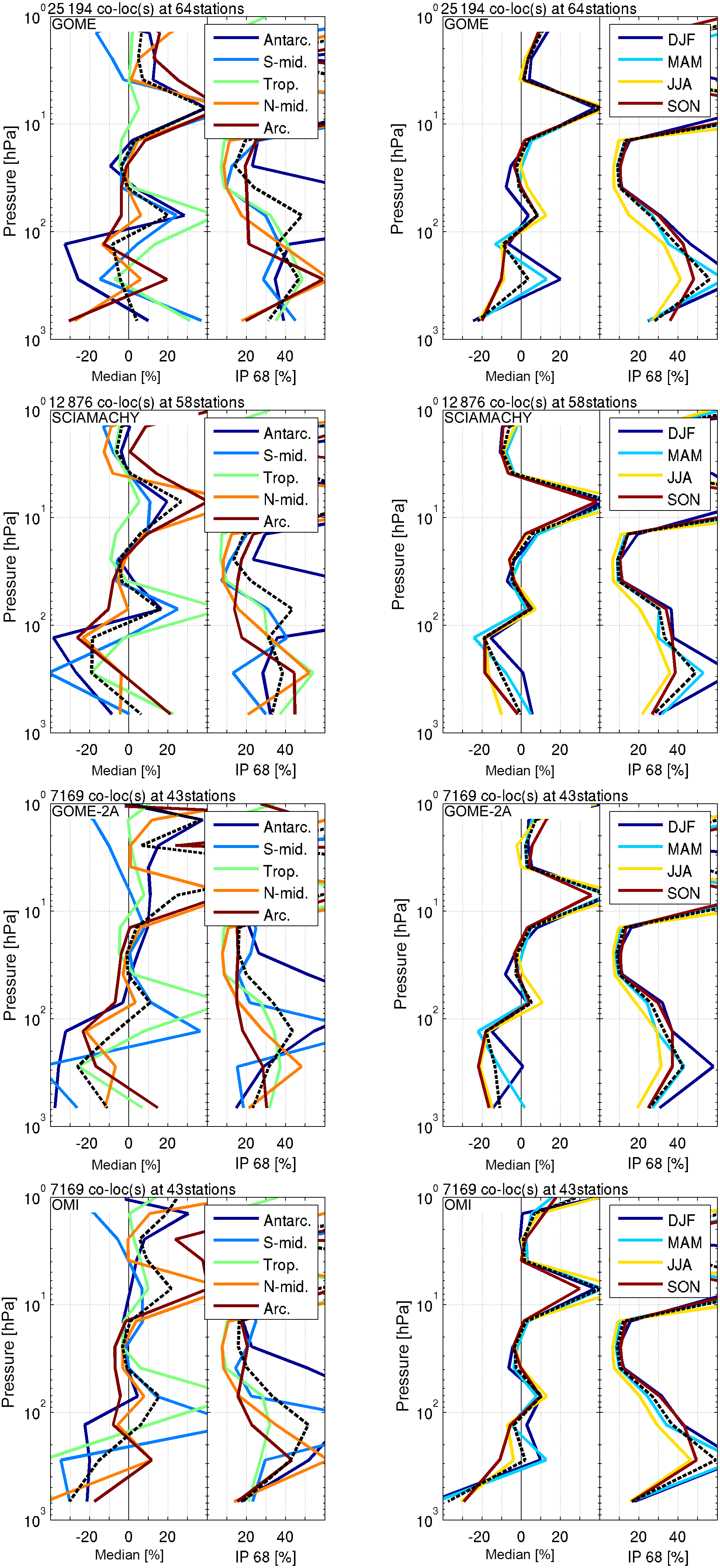
Figure 11Median relative differences and 68 % interpercentile spreads for comparison of L3 GOME, SCIAMACHY, GOME-2A, and OMI data (top to bottom panels) with ground-based reference measurements. The same difference statistics are redistributed in each line over two influence quantity ranges, with the influence quantities being the latitude (left panels) and quarter (right panels). The black dashed line shows the average of the coloured curves.
GOME L3 data show an above-tropopause bias of 5–10 % positive to negative, with strong outliers around 70 and 8 hPa, especially in the tropical UTLS and Antarctic local spring (up to 50 %) due to ozone hole's vortex conditions. The corresponding spread is of the order of 10–30 %, with again outliers at the same two scenes. Especially during Antarctic spring (SON) the spread explodes to the order of 100 %. Below the tropopause (100–200 hPa), GOME L3 data show stronger negative and positive biases ranging between 10 and 30 %. Exceptions can be observed in the Arctic winter (DJF) and Antarctic spring (SON), with outliers ranging up to 60 and −50 %, respectively. Corresponding spread values are of the order of 20–40 %, with the highest values again in Arctic winter.
The SCIAMACHY L3 bias and spread values are very similar to those of the GOME L3 comparison results. Only exceptions are the strong positive Arctic spring (MAM) bias in the troposphere (up to 40 %) and the availability of Antarctic winter (JJA) data showing a strong negative bias in the UTLS and above (−30 to −40 %). Also the GOME-2 instrument on board Metop-A shows a performance that is very similar to the GOME instrument in terms of L3 bias and spread. The only significant difference is in the bias during the northern and southern DJF quarter: GOME-2A outliers are much more negative (up to −50 %) for the lowest partial columns. OMI's L3 bias and spread again are very similar to those of the other three instruments, with the difference that the negative tropical tropospheric bias is more pronounced (−40 %) and a positive tropospheric bias (30–50 %) is introduced in the Southern Hemisphere during local winter (JJA).
Overall one could state that between about 10 hPa and the tropopause (100–200 hPa), relative differences and spreads are of the order of −5 and 10–30 %, respectively, for all four instruments, while the troposphere shows a 10–40 % bias (both positive and negative) and spread. Strong outliers do occur, typically in the troposphere of the Arctic winter (DJF), in the equatorial UTLS (order of 50 % positive for all seasons and instruments), and in the Antarctic local winter (JJA) and spring (SON) due to strong ozone variability around the polar vortex.
5.4 UV–VIS L2 and L3 drift studies
Relative decadal drift and 68 % interpercentile spreads for comparisons of L2 and L3 GOME, SCIAMACHY, GOME-2A, and OMI data with ground-based reference measurements are collected in Fig. 12. As discussed in the previous section for their bias and spread behaviour, the similarity between the L2 and L3 UV–VIS drift results for the same instrument appears very clearly. Again, however, features in the L2 statistics are enlarged for the L3 data due to larger differences in spatiotemporal representativeness (except for the lowest-level spread, see previous section).
The GOME L2 and L3 stratospheric drift typically do not exceed 10 % decade−1 values, with the exception of an almost 20 % decade−1 positive drift near the South Pole lower stratosphere and an equally large L3 peak around 35 km. Only the latter is clearly significant in terms of the corresponding 95 % drift confidence interval (CI, as horizontal error bars). This can also be observed from the highly peaked (> 60 %) IP68 spread on the differences (right-hand panel in each plot of Fig. 12). This peak indeed partially reflects the instrument's drift, as the spread is not determined from the drift residuals but with respect to the overall median difference. A large drift will as such contribute to a large spread. The negative drift values appearing above 45 km are considered less trustworthy because of the sparseness of the lidar reference data. The GOME tropospheric drift equals about −5 % decade−1 on average, but at the lowest altitudes ranges from −20 % decade−1 at the South Pole to 20 % decade−1 near the Equator. Yet again the L2 drifts remain within the CI and are therefore insignificant.
SCIAMACHY drift results strongly differ from the GOME observations: although still mostly insignificant, the above-tropopause drift is of the order of −10 % decade−1 and shows the same L3 outlier at 35 km. Below the tropopause, however, the drift ranges from about 20 % decade−1 at the poles to 50–60 % decade−1 towards the Equator. This entails that in the mid-latitudes (both north and south) and tropics this drift is significant. The GOME-2A drift results come close to the SCIAMACHY drift performance, although the sub-tropopause drift is even stronger (around 50 % decade−1) and significant globally. Besides, a significant negative drift of the order of 30 % decade−1 also appears in the UTLS, which is strongest around the Equator, reaching −70 % decade−1 around 100 hPa.
Despite the occurrence of insignificant negative drifts in the Northern Hemisphere, the OMI L3 tropospheric drift is significantly positive (around 40 % decade−1 on average) in the Southern Hemisphere and the tropics, resulting in a global average L3 tropospheric drift of the order of 15 % decade−1 (see Fig. 12). The L2 tropospheric drift equals about 5 to 10 % decade−1 only and is close to insignificant. It is remarkable that the OMI L3 drift is typically 10 % negative in the UTLS (with −40 % decade−1 values around the Equator), while in the stratosphere above an average 10 % decade−1 positive drift can be observed. Both L2 and L3 show a negative close to 20 % decade−1 value just below 40 km. These results and their significance are in qualitative agreement with Huang et al. (2017) on the OMI PROFOZ retrieval product.
On the global scale, as shown in Fig. 12, the decadal drift is order of 5 % negative and insignificant for GOME and order of −15 and 10 % insignificant (except for the tropics) for OMI's L2 stratosphere and troposphere, respectively. A significant positive drift of the order of 40 % decade−1 is observed for SCIAMACHY and GOME-2A below the tropopause. GOME-2A moreover shows a significant 30 % decade−1 negative drift in the UTLS at all latitudes.
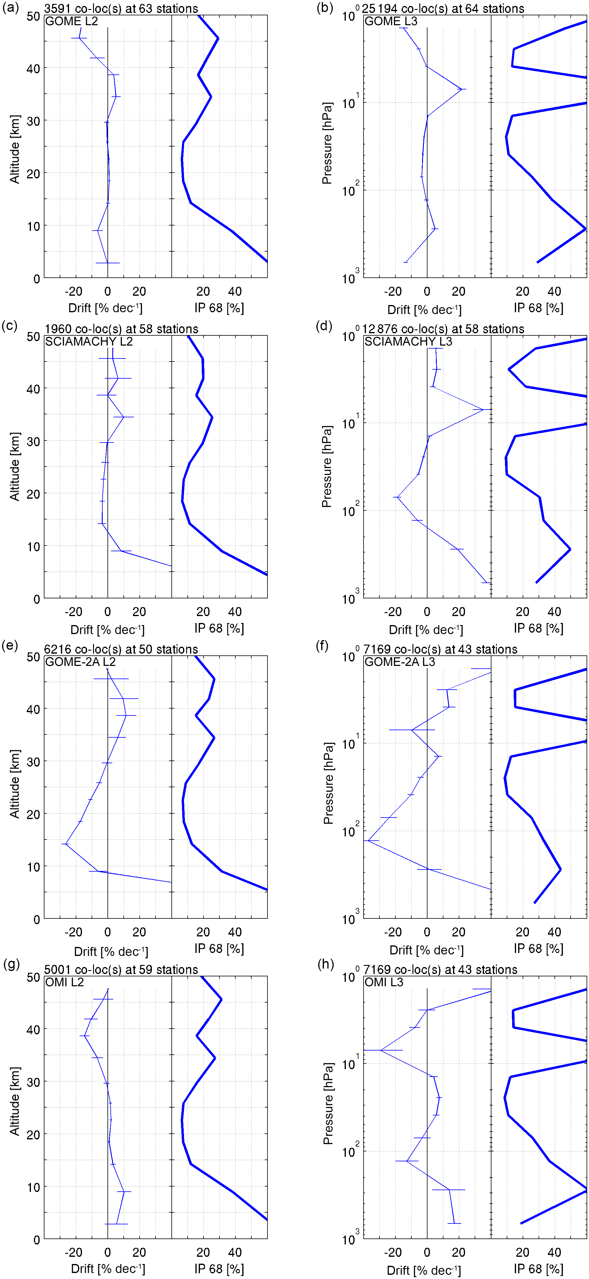
Figure 12Relative decadal drift and 68 % interpercentile spreads for comparisons of L2 (a, c, e, g) and L3 (b, d, f, h) GOME, SCIAMACHY, GOME-2A, and OMI data (top to bottom panels) with ground-based reference measurements. Two sigma error bars, resulting from a bootstrapping with 1000 samples, are added to the drift profiles.
5.5 L4 assimilated data
The L4 1996–2013 data, constructed by data assimilation at KNMI from merged RAL v2.14 GOME and GOME-2A observations, can be compared with ground-based reference profiles directly. The single 2 × 3∘ box that overlaps with the ground measurement within 3 h is thereby taken as the co-located measurement. The number of co-locations and stations, however, is smaller than for the L3 data, as data from 64 ozonesonde stations (that have been used for satellite bias correction during assimilation) are omitted from the comparative analysis. Median relative differences and 68 % interpercentile spreads for comparison of the L4 assimilated nadir ozone profile data with ground-based reference measurements are collected in Fig. 13, redistributed over two influence quantity ranges (latitude and quarter). The corresponding relative decadal drift and overall 68 % interpercentile spread profiles are added as well.
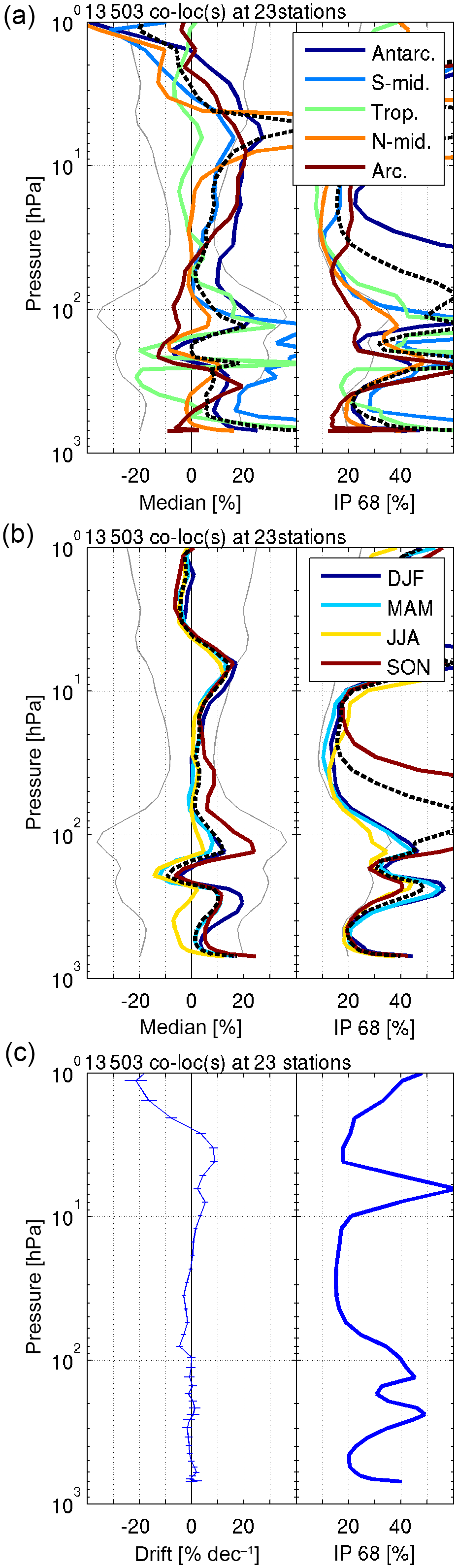
Figure 13Median relative differences and 68 % interpercentile spreads for comparison of L4 assimilated nadir ozone profile data with ground-based reference measurements (a, b). The same difference statistics are redistributed over two influence quantity ranges, with the influence quantities being the latitude (a) and quarter (b). The black dashed line shows the average of the coloured curves, while light grey lines indicate the satellite uncertainty provided in the product. Panel (c) shows the corresponding relative decadal drift and 68 % interpercentile spread. Two sigma error bars, resulting from a bootstrapping with 1000 samples, are added to the drift profile.
The most remarkable result that can be observed from the UV–VIS L4 comparison statistics is that, as a result of the model assimilation, the typical Z-shape of the L2 bias has disappeared. The L4 bias typically remains below 10 % (positive and negative) with the exception of a strong positive outlier around 5 hPa (as for the L3 data) and the surface boundary layer and a 20 % positive to negative fluctuation around the UTLS that is strongest in the tropics (∼ 50 % positive for all seasons, with a similar but only positive bias feature in the Southern Hemisphere). This entails that the L2 and L3 comparison features in the Antarctic spring (SON) with ozone hole conditions and in most of the troposphere have been strongly reduced. The L4 spread remains close to the L2 and L3 values, though with an even stronger reduction (to 20 %) in the troposphere than the L3 comparisons as no monthly averages are considered. Moreover, due to the ozonesonde-based bias correction the remaining L4 drift is of the order of a few percent only and insignificant, i.e. within the 95 % CI, for all altitudes up to about 40 km globally.
5.6 L2 TIR nadir ozone profiles
Similarly to the L2 RAL v2.14 UV–VIS retrievals, Figs. 14 and 15 contain the median relative differences, 68 % interpercentile spreads, and vertical sensitivities for the comparison of FORLI v20151001 retrieved IASI profiles with ground-based reference measurements (IASI-A for 2008–2015, IASI-B for 2013–2015). Difference and information statistics are again redistributed in each plot over several influence quantity ranges, with the influence quantities now being the latitude, quarter, total ozone column (DU), DFS, SZA, SPI, and TC. For IASI-A in Fig. 14, the corresponding relative decadal drift and overall 68 % interpercentile spread are also added.
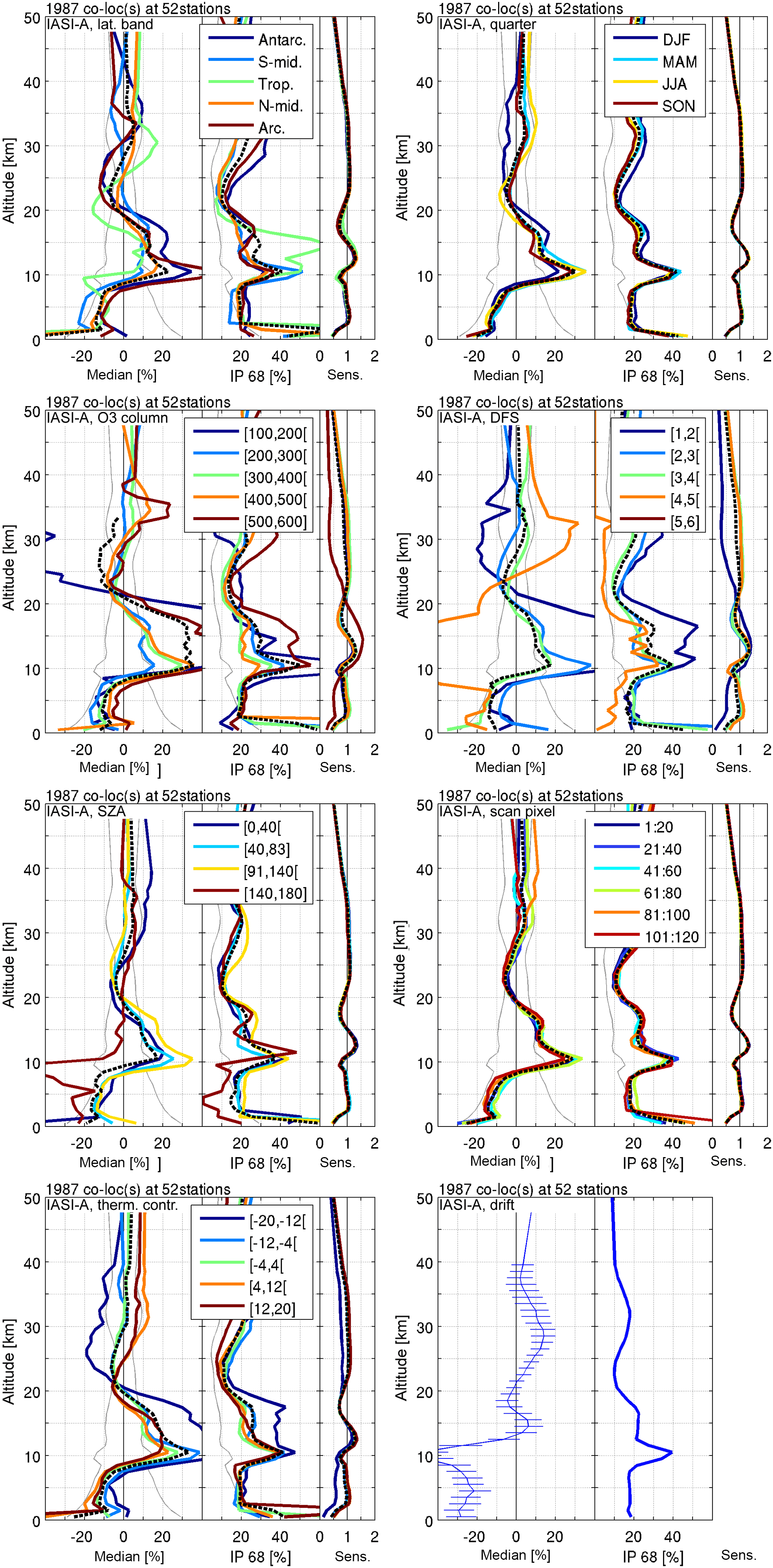
Figure 14Median relative differences, 68 % interpercentile spreads, and vertical sensitivities for comparison of FORLI v20151001 L2 IASI-A retrieved profiles with ground-based reference measurements (2008–2015). The same difference and information statistics are redistributed in each plot over several influence quantity ranges, with the influence quantities being (from left to right and top to bottom) latitude, quarter, total ozone column (DU), DFS, SZA, SPI, and TC. In the corresponding legend entries, open brackets are used to indicate that the last value is not included (i.e. values in the set go up to, but do not equal, the last value). The black dashed line shows the average of the coloured curves, while light grey lines indicate the satellite uncertainty provided in the product. The bottom right plot contains the corresponding relative decadal drift and 68 % interpercentile spread. Two sigma error bars, resulting from a bootstrapping with 1000 samples, are added to the drift profile.
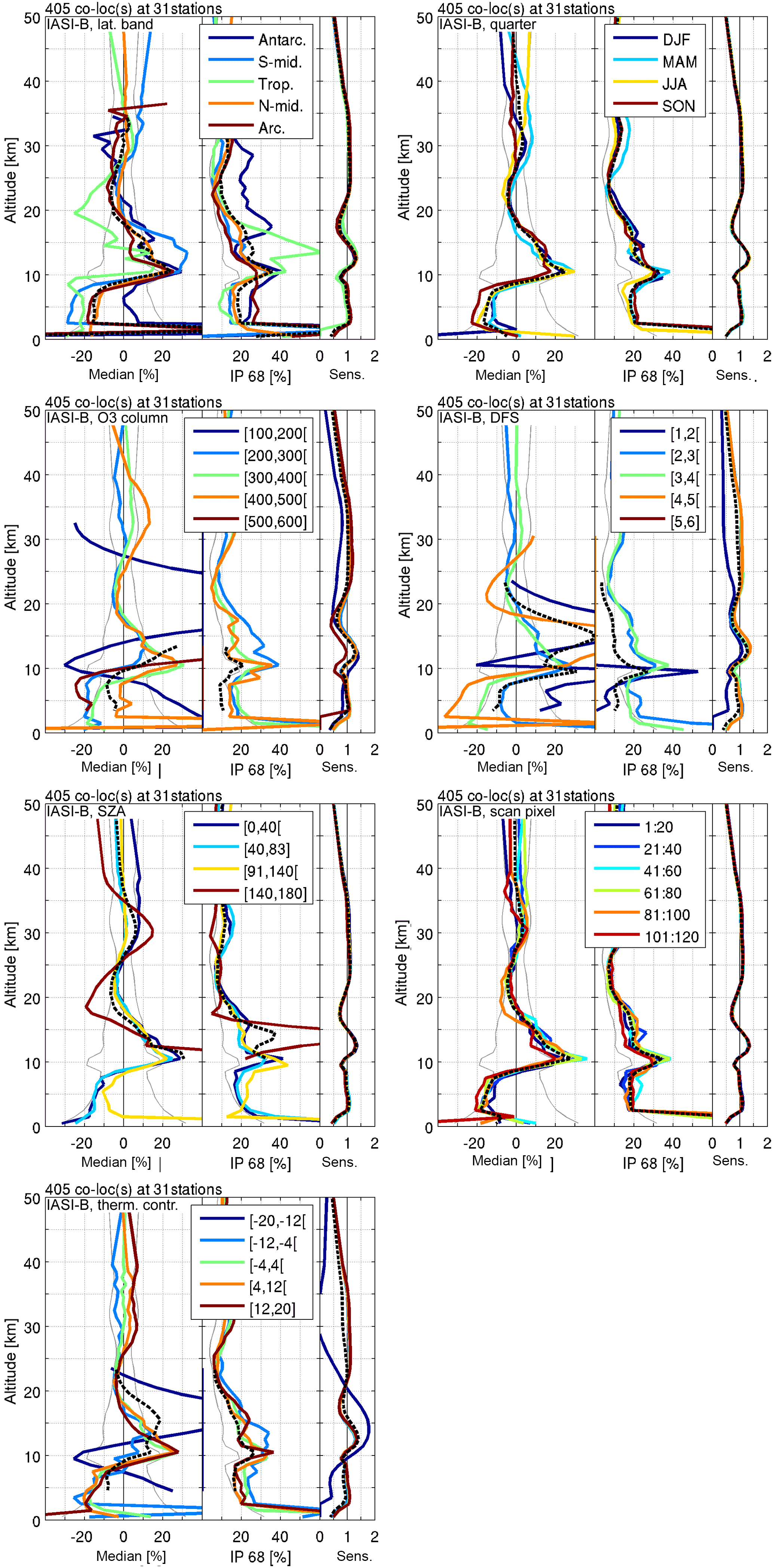
Figure 15As for Fig. 14, but for FORLI v20151001L2 IASI-B data (2013–2015). Because of the limited temporal extent of this product, no drift study has been performed.
As already pointed out in the information content studies, the IASI-A and IASI-B results are very similar, showing no significant differences between their respective statistics. Overall the FORLI v20151001 IASI retrieval data products show a less than 10 % and insignificant stratospheric bias, a 10 to 30 % positive bias in the UTLS, and an order of 10 % negative bias in the troposphere. The latter is in agreement with an initial IASI tropospheric ozone (also retrieved with FORLI v20151001) validation exercise using ozonesonde reference measurements performed by Boynard et al. (2016). Possible reasons for the UTLS bias are discussed in Dufour et al. (2012). Taking into account the FRM uncertainties discussed in Sect. 3.2, the ex ante IASI uncertainties provided in the product files (light grey lines in the plots) are typically of the order of the bias, except in the UTLS. The ex post random uncertainty, as estimated by the spread, is roughly twice as large, except for the lower tropics. This means that overall the total satellite measurement and retrieval uncertainty is underestimated in the IASI FORLI v20151001 nadir ozone profile products. The comparison results show hardly any scan angle dependence or seasonality, except for some larger systematic differences around the Antarctic ozone hole that can be partially attributed to co-location errors at the edge of the polar vortex. The remaining meridian dependences are typically limited to stronger UTLS bias fluctuations in the tropics.
Both the polar sub-tropopause and tropical UTLS outliers seem to go together with a TC dependence of the differences (clearer for IASI-A than for IASI-B) that also agrees with the sensitivity dependence. One would expect the TC to be mainly influential in the lowermost layers, but the information content studies on the IASI product have indeed demonstrated that the corresponding averaging kernels show significant vertically interdependent oscillations. Therefore the polar sensitivity outliers around 30 km altitude can be related to the strongly negative thermal contrasts and typically go together with very low DFS values (below two, suggesting screening upon this threshold) and strong ozone overestimations. The latter is again clearer for the longer IASI-A time series, wherein the highest total ozone column profiles have the lowest DFS values. Finally, differences can be observed between the IASI daytime (SZA < 83∘) and nighttime (SZA > 91∘) measurements, which are most clear for the largest SZAs (140 to 180∘). Due to the small numbers of co-locations for the latter, however, it is difficult to attribute any significance to these differences.
Looking at latitude-resolved drift studies for the Ozone_cci IASI-A nadir ozone profiles (not shown), a significant decadal negative drift of the order of 25 % or higher can be observed in the Antarctic UTLS and the northern hemispheric troposphere. On the global scale (see Fig. 14), the significance of these drifts remains in terms of the corresponding 95 % drift confidence intervals (horizontal error bars) and is again reflected in the peaked UTLS IP68 spread on the differences (40 %) as the spread is not determined from the drift residuals but with respect to the overall median difference. A less pronounced positive drift is detected around 30 km altitude. Part of the overall negative tropospheric drift of the FORLI v20151001 IASI retrievals could, however, be due to a change in the processing of the IASI L2 processor (e.g. temperature profile) at EUMETSAT that changed to version 5.0.6 in September 2010. This idea is supported by Boynard et al. (2017), who have observed that the IASI-A FORLI v20151001 tropospheric drift becomes statistically insignificant if calculated from the September 2010 to 2016 period retrievals only.
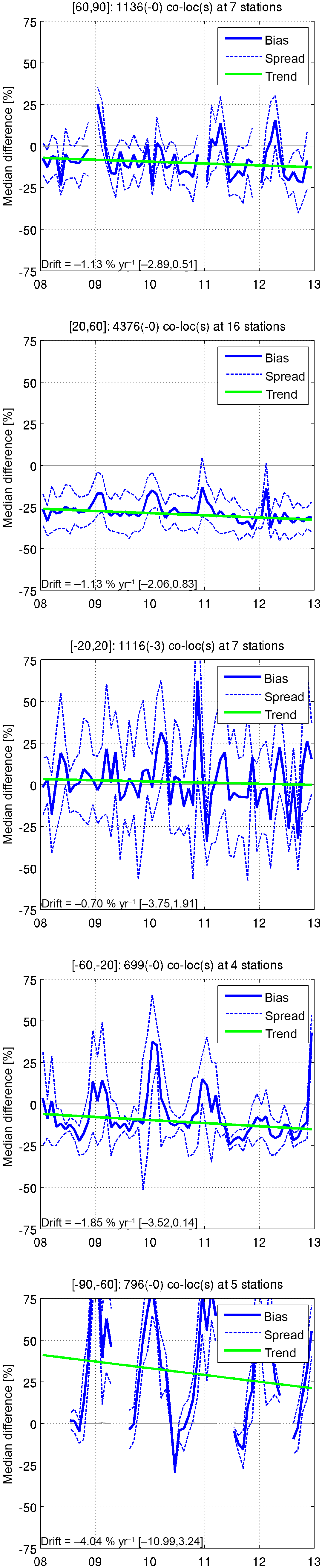
Figure 16Time series of the median bias (solid blue), spread (dashed blue), and linear drift (green line) for direct comparisons of IASI L3 monthly gridded mean tropospheric ozone column data (0 to 6 km) with vertically integrated ozonesonde reference data (at stations with at least six launches per month), divided into five latitude bands (sorted north to south). The number of filtered values is added between brackets in the title of each plot, while the yearly linear drift value and its 95 % confidence interval are added in the lower-left corner.
5.7 L3 TIR monthly gridded tropospheric ozone product
Time series of median relative differences (in solid blue), spreads (in dashed blue), and linear drift (green) for direct comparisons of the IASI-A L3 monthly gridded mean tropospheric ozone column data (integrated from 0 to 6 km) with integrated ozonesonde reference data (at stations with at least six valid measurements per month) are determined within five latitude bands and plotted in Fig. 16. The yearly linear drift value and its 95 % confidence interval as an uncertainty estimate on the derived slope are both determined from a bootstrapping technique using 1000 subsamples and are added in the lower-left corner of each graph.
The IASI-A TIR monthly gridded tropospheric ozone column data for January 2008 to December 2012 show a strong seasonal variation in their comparison with the integrated ozonesonde data, ranging up to 100 %, especially around the South Pole. Despite this strong seasonality, and in agreement with the IASI-A L2 comparison statistics, median relative differences throughout the whole time series range between 25 % negative in the northern mid-latitudes and 30 % positive in Antarctica, with a nearly zero overall bias around the Equator. The corresponding spread decreases from about 25 % in the tropics to about 5–10 % towards the poles. The drift, however, increases from less than 1 % per year negative in the tropics to up to −4 % per year around the South Pole. In contrast with the IASI-A L2 drift study results, none of these drifts are significant, as the 95 % confidence intervals in combination with the comparison spreads indicate: where the confidence interval is fully negative, as is the case for the mid-latitudes, the distance of the confidence interval from zero drift is much smaller than the average spread on the differences. This difference between the IASI L2 and L3 significance of the drift is mainly due to their difference in spatiotemporal representativeness with respect to the ground-based reference data (averaging kernel smoothing, vertical integration, and monthly averaging).
Table 5Major QA and validation quantities, their corresponding typical values, and indication of GCOS user requirement (UR) compliance for the Ozone_cci nadir ozone profile CRDP.
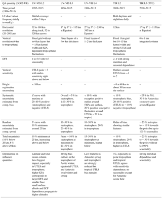
Table 5 summarizes the major QA and validation quantities discussed throughout this work, their corresponding typical values as discussed in the previous sections, and provides associated GCOS user requirements for the entire Ozone_cci nadir ozone profile CRDP, meaning that UV–VIS and TIR measurement and retrieval-based products are combined. These 13 ozone ECV datasets together cover the 1995 to 2015 time period globally, which is sufficiently long for (drift-corrected) ozone trend studies according to the GCOS user requirements. Yet the ongoing and upcoming satellite observations of both the GOME type (GOME-2 on Metop-A/B, Sentinel-5 Precursor TROPOMI, and the upcoming Copernicus Sentinel-5 series) and the IASI type (IASI on Metop platforms and IASI-NG on Metop-SG platforms) will even extend the available time series. Expecting a similar or even improved quality for these data in terms of information content, total uncertainty, and especially horizontal resolution (cf. Sentinel-5p with a 7 km by 7 km ground pixel), the Ozone_cci CRDP seems fit for long-term vertically resolved ozone climate monitoring and modelling as e.g. done in the TOAR, the WMO/UNEP Ozone Depletion Assessment, and the SPARC LOTUS initiative. All nadir ozone profile products under study indeed also fulfil the GCOS user requirements in terms of observation frequency and horizontal and vertical resolution. Only for the latter does one have to keep in mind that all L2 nadir ozone profile observations show UTLS sensitivity outliers and are strongly correlated vertically due to averaging kernel fluctuations that extend far beyond the (typically tropospheric) kernel's 15 km FWHM.
The Ozone_cci CRDP nadir ozone profile products typically do not comply with the GCOS user requirements in terms of total uncertainty and decadal drift. The total uncertainty is thereby determined as the quadratic sum of the products' systematic and random uncertainties, which on their turn are estimated from the comparison (with ground-based reference measurement) bias and spread, respectively. Note that this as a conservative estimate, as the bias and spread also include uncertainties due to smoothing and sampling differences between the satellite data and the FRM. Whereas the RAL v2.14 UV–VIS retrieved products show a typical Z-curve bias with strong 20–40 % positive (stratosphere) and negative (UTLS) maxima, the FORLI v20151001 systematic uncertainty is rather consistently of the order of 10 % in the stratosphere and troposphere, but shows stronger fluctuations (20 to 40 %) in the (especially tropical) UTLS. Total uncertainties therefore range from about 10 % at minimum in the stratosphere to at least 20 % in the troposphere (for IASI), and even higher values in the UTLS and for the UV–VIS instruments. Comparison statistics for the L3 monthly gridded averages are obviously of the same order, but L2 features can be both enlarged or reduced due to clear differences in spatiotemporal representativeness (also with the FRM data). KNMI's L4 data contain a remaining 10 % bias, with the exception of a positive outlier around 5 hPa and near the Earth's surface, and an order of 20 % fluctuation around the UTLS that increases to about 50 % in the tropics.
Drift studies for all nadir ozone profile CRDP products (except for the Metop-B instruments) show that the 1 to 3 % decade−1 GCOS requirement is only met by the L4 UV–VIS data. The higher drift values are found to be mostly insignificant for the L2 GOME and OMI instrument retrievals and for the L3 TIR data. The SCIAMACHY and GOME-2A products have a strong positive drift (up to 40 %) in the troposphere, and GOME-2A moreover shows a 20 % decade−1 negative drift around the tropopause. The FORLI IASI-A instrument retrieval shows an order of 25 % significant negative drift in the Antarctic UTLS and northern hemispheric troposphere only. Together with the systematic uncertainty studies, these drift results call for an appropriate altitude-dependent bias and drift correction of the L2 Ozone_cci nadir ozone profile products by data users for climate and atmospheric composition monitoring and modelling purposes.
Applying bias and drift corrections to the nadir ozone profile CRDP presented in this work straightforwardly might not yield optimal results. Next to the L2 data screening recommended by the respective data providers as summarized in Table 3, the validation results presented in the previous sections point at additional data screening options. In the UV–VIS instrument datasets (except for GOME-2B), some satellite profiles with very low DFS, nearly zero stratospheric sensitivity, and high bias occur, mainly around the SAA. By inserting a DFS < 3 flag, for example, these profiles could be fully screened or considered for tropospheric ozone monitoring only. The latter would be equivalent to an altitude-dependent screening, which could also be used along with the full-profile effective cloud screening advised by the RAL team. Comparison results have shown that one could apply a layer screening up to the UTLS instead, as the stratospheric ozone retrieval is hardly affected by the ECF (or surface albedo). Analogously, the bias outliers for the FORLI v20151001 IASI retrievals in the polar troposphere and the tropical UTLS go together with a TC and sensitivity dependence of the differences. These profiles could therefore be excluded from any further use by insertion of a strongly negative TC or low DFS value screening, e.g. shifting the DFS screening threshold from one (as suggested by the ULB–LATMOS retrieval team) to two. As for the RAL data, vertically resolved profile screening could additionally reject consistent altitude-dependent bias or drift outliers.
This work, the second in a series of four Ozone_cci papers, reports for the first time on data content studies, information content studies, and comparisons with co-located ground-based reference observations for all 13 nadir ozone profile data products that are part of the CRDP on atmospheric ozone of the European Space Agency's Climate Change Initiative. These products consist of five L2 UV–VIS instrument retrieval datasets, two L2 TIR retrieval datasets, four UV–VIS L3 monthly gridded data series, a merged UV–VIS L4 product, and a 0 to 6 km integrated tropospheric L3 product based on IASI-A data. To verify their fitness for purpose and especially their compliance with the requirements identified for the GCOS, these ozone datasets were subjected to a comprehensive quality assessment system developed in several heritage projects. The ground-based reference measurements have thereby been taken from the well-established NDACC, SHADOZ, and WMO GAW ozonesonde and lidar networks. All nadir ozone profile products under study fulfil the GCOS user requirements in terms of observation frequency and horizontal and vertical resolution. Yet all L2 nadir ozone profile observations also show sensitivity outliers in the UTLS and are strongly correlated vertically due to substantial averaging kernel fluctuations that extend far beyond the (typically tropospheric) kernel's 15 km FWHM. However, the required observation period for climate modelling is only fully covered when several instrument time series are combined. Moreover, the nadir ozone profile CRDP typically does not comply with the GCOS user requirements in terms of total uncertainty and decadal drift (except for the UV–VIS L4 dataset). The drift values of the L2 GOME and OMI, the L3 IASI, and the L4 assimilated products are found to be overall insignificant, and applying appropriate altitude-dependent bias and drift corrections make the data fit for climate and atmospheric composition monitoring and modelling purposes. The nadir ozone profile product validation in terms of several influence quantities presented in this work correspondingly calls for the introduction of one or more L2 profile flags in addition to those recommended by the data providers, majorly based on a lower DFS threshold.
The ESA Ozone_cci datasets are available at http://www.esa-ozone-cci.org/?q=node/160 (last access: 18 June 2018). The ground-based ozonesonde and lidar data used in this publication were obtained as part of WMO's Global Atmospheric Watch (GAW) programme, including the Network for the Detection of Atmospheric Composition Change (NDACC) and NASA's Southern Hemisphere Additional Ozonesonde programme (SHADOZ), and they are publicly available via the NDACC Data Host Facility (http://www.ndsc.ncep.noaa.gov/data/, last access: 18 June 2018; De Mazière et al., 2018), the SHADOZ archive (https://tropo.gsfc.nasa.gov/shadoz/Archive.html, last access: 18 June 2018; Thompson et al., 2012), and the World Ozone and Ultraviolet Data Centre (WOUDC) archive (https://woudc.org/data/explore.php, last access: 18 June 2018).
The authors declare that they have no conflict of interest.
This article is part of the special issue “Quadrennial Ozone Symposium 2016 – Status and trends of atmospheric ozone (ACP/AMT inter-journal SI)”. It is a result of the Quadrennial Ozone Symposium 2016, Edinburgh, United Kingdom, 4–9 September 2016.
The reported work was funded by ESA via the CCI–ECV Ozone project, with
support from the Belgian Federal Science Policy Office (BELSPO) and ProDEx
via project A3C. We made use of the versatile Multi-TASTE validation system
which was developed in heritage projects and refined recently within the
FP7 EU Project Quality Assurance for Essential Climate Variables (QA4ECV), grant
no. 60740. We warmly thank several members of the NDACC ozonesonde and lidar working
groups for fruitful discussions. Lidar operation is funded through national
collaborators and we are grateful to the following institutes and their
co-workers who contributed to generating these data: CNRS and CNES (Dumont
d'Urville station and Observatoire Haute Provence; PI is Sophie Godin-Beekmann),
DWD (Höhenpeißenberg station; PI is Hans Claude), RIVM and NIWA
(Lauder station; PIs are Daan P. J. Swart and Richard Querel), NASA/JPL (Mauna Loa
Observatory and Table Mountain Facility; PIs are Russell C. Schnell and Thierry Leblanc),
and NIES (Tsukuba station; PI is Hideaki Nakane).
Edited by: Irina Petropavlovskikh
Reviewed by: two anonymous referees
Anderson, G. P., Barth, C. A., Cayla, F., and London, J.: Satellite observations of the vertical ozone distribution in the upper stratosphere, Annales de Géophysique, 25, 341–345, 1969.
August, T., Klaes, D., Schlüssel, P., Hultberg, T., Crapeau, M., Arriaga, A., O'Carroll, A., Coppens, D., Munro, R., and Calbet, X.: IASI on Metop-A: Operational Level 2 retrievals after five years in orbit, J. Quant. Spectrosc. Ra., 113, 1340–1371, https://doi.org/10.1016/j.jqsrt.2012.02.028, 2012.
Boynard, A., Hurtmans, D., Koukouli, M. E., Goutail, F., Bureau, J., Safieddine, S., Lerot, C., Hadji-Lazaro, J., Wespes, C., Pommereau, J.-P., Pazmino, A., Zyrichidou, I., Balis, D., Barbe, A., Mikhailenko, S. N., Loyola, D., Valks, P., Van Roozendael, M., Coheur, P.-F., and Clerbaux, C.: Seven years of IASI ozone retrievals from FORLI: validation with independent total column and vertical profile measurements, Atmos. Meas. Tech., 9, 4327–4353, https://doi.org/10.5194/amt-9-4327-2016, 2016.
Boynard, A., Hurtmans, D., Garane, K., Goutail, F., Hadji-Lazaro, J., Koukouli, M. E., Wespes, C., Keppens, A., Pommereau, J.-P., Pazmino, A., Balis, D., Loyola, D., Valks, P., Coheur, P.-F., and Clerbaux, C.: Validation of the IASI FORLI/Eumetsat ozone products using satellite (GOME-2), ground-based (Brewer–Dobson, SAOZ) and ozonesonde measurements, Atmos. Meas. Tech. Discuss., https://doi.org/10.5194/amt-2017-461, in review, 2018.
Burrows, J. P., Weber, M., Buchwitz, M., Rozanov, V., Ladstätter-Weißenmayer, A., Richter, A., DeBeek, R., Hoogen, R., Bramstedt, K., Eichmann, K., Eisinger, M., and Perner, D.: The Global Ozone Monitoring Experiment (GOME): Mission Concept and First Scientific Results, J. Atmos. Sci., 56, 151–175, https://doi.org/10.1175/1520-0469(1999)056<0151:TGOMEG>2.0.CO;2, 1999.
Dee, D. P., Uppala, S. M., Simmons, A. J., Berrisford, P., Poli, P., Kobayashi, S., Andrae, U., Balmaseda, M. A., Balsamo, G., Bauer, P., Bechtold, P., Beljaars, A. C. M., van de Berg, L., Bidlot, J., Bormann, N., Delsol, C., Dragani, R., Fuentes, M., Geer, A. J., Haimberger, L., Healy, S. B., Hersbach, H., Hólm, E. V., Isaksen, L., Kållberg, P., Köhler, M., Matricardi, M., McNally, A. P., Monge-Sanz, B. M., Morcrette, J.-J., Park, B.-K., Peubey, C., de Rosnay, P., Tavolato, C., Thépaut, J.-N., and Vitart, F.: The ERA-interim reanalysis: configuration and performance of the data assimilation system, Q. J. Roy. Meteorol. Soc., 137, 553–597, https://doi.org/10.1002/qj.828, 2011.
De Mazière, M., Thompson, A. M., Kurylo, M. J., Wild, J. D., Bernhard, G., Blumenstock, T., Braathen, G. O., Hannigan, J. W., Lambert, J.-C., Leblanc, T., McGee, T. J., Nedoluha, G., Petropavlovskikh, I., Seckmeyer, G., Simon, P. C., Steinbrecht, W., and Strahan, S. E.: The Network for the Detection of Atmospheric Composition Change (NDACC): history, status and perspectives, Atmos. Chem. Phys., 18, 4935–4964, https://doi.org/10.5194/acp-18-4935-2018, 2018.
Donlon, C. and Zibordi, G.: In Situ Optical Radiometry, in: chap. 3 of Optical Radiometry for Ocean Climate Measurements, Experimental Methods in the Physical Sciences Series, Vol. 47, edited by: Zibordi, G., Donlon, C., and Parr, A., Elsevier Inc., London, UK, 2014.
Dufour, G., Eremenko, M., Griesfeller, A., Barret, B., LeFlochmoën, E., Clerbaux, C., Hadji-Lazaro, J., Coheur, P.-F., and Hurtmans, D.: Validation of three different scientific ozone products retrieved from IASI spectra using ozonesondes, Atmos. Meas. Tech., 5, 611–630, https://doi.org/10.5194/amt-5-611-2012, 2012.
Flynn, L. E., Seftor, C. J., Larsen, J. C., and Xu, P.: The Ozone Mapping and Profiler Suite, in: Earth Science Satellite Remote Sensing, edited by: Qu, J. J., Gao,W., Kafatos, M., Murphy, R. E., and Salomonson, V. V., Springer, Berlin, 279–296, https://doi.org/10.1007/978-3-540-37293-6, 2006.
Garane, K., Lerot, C., Coldewey-Egbers, M., Verhoelst, T., Koukouli, M. E., Zyrichidou, I., Balis, D. S., Danckaert, T., Goutail, F., Granville, J., Hubert, D., Keppens, A., Lambert, J.-C., Loyola, D., Pommereau, J.-P., Van Roozendael, M., and Zehner, C.: Quality assessment of the Ozone_cci Climate Research Data Package (release 2017) – Part 1: Ground-based validation of total ozone column data products, Atmos. Meas. Tech., 11, 1385–1402, https://doi.org/10.5194/amt-11-1385-2018, 2018.
Heath, D. F., Mateer, C. L., and Krueger, A. J.: The Nimbus-4 Backscatter Ultraviolet (BUV) Atmospheric Ozone Experiment-Two Years' Operation, Pure Appl. Geophys., 106–108, 1238–1245, 1973.
Heath, D. F., Krueger, A. J., Roeder, H. A., and Henderson, B. D.: Solar Backscatter Ultraviolet and Total Ozone Mapping Spectrometer (SBUV-TOMS) for Nimbus G, Opt. Eng., 14, 323–331, 1975.
Huang, G., Liu, X., Chance, K., Yang, K., Bhartia, P. K., Cai, Z., Allaart, M., Ancellet, G., Calpini, B., Coetzee, G. J. R., Cuevas-Agulló, E., Cupeiro, M., De Backer, H., Dubey, M. K., Fuelberg, H. E., Fujiwara, M., Godin-Beekmann, S., Hall, T. J., Johnson, B., Joseph, E., Kivi, R., Kois, B., Komala, N., König-Langlo, G., Laneve, G., Leblanc, T., Marchand, M., Minschwaner, K. R., Morris, G., Newchurch, M. J., Ogino, S.-Y., Ohkawara, N., Piters, A. J. M., Posny, F., Querel, R., Scheele, R., Schmidlin, F. J., Schnell, R. C., Schrems, O., Selkirk, H., Shiotani, M., Skrivánková, P., Stübi, R., Taha, G., Tarasick, D. W., Thompson, A. M., Thouret, V., Tully, M. B., Van Malderen, R., Vömel, H., von der Gathen, P., Witte, J. C., and Yela, M.: Validation of 10-year SAO OMI Ozone Profile (PROFOZ) product using ozonesonde observations, Atmos. Meas. Tech., 10, 2455–2475, https://doi.org/10.5194/amt-10-2455-2017, 2017.
Hubert, D., Lambert, J.-C., Verhoelst, T., Granville, J., Keppens, A., Baray, J.-L., Bourassa, A. E., Cortesi, U., Degenstein, D. A., Froidevaux, L., Godin-Beekmann, S., Hoppel, K. W., Johnson, B. J., Kyrölä, E., Leblanc, T., Lichtenberg, G., Marchand, M., McElroy, C. T., Murtagh, D., Nakane, H., Portafaix, T., Querel, R., Russell III, J. M., Salvador, J., Smit, H. G. J., Stebel, K., Steinbrecht, W., Strawbridge, K. B., Stübi, R., Swart, D. P. J., Taha, G., Tarasick, D. W., Thompson, A. M., Urban, J., van Gijsel, J. A. E., Van Malderen, R., von der Gathen, P., Walker, K. A., Wolfram, E., and Zawodny, J. M.: Ground-based assessment of the bias and long-term stability of 14 limb and occultation ozone profile data records, Atmos. Meas. Tech., 9, 2497–2534, https://doi.org/10.5194/amt-9-2497-2016, 2016.
Hurtmans, D., Coheur, P.-F., Wespes, C., Clarisse, L., Scharf, O., Clerbaux, C., Hadji-Lazaro, J., George, M., and Turquety, S.: FORLI radiative transfer and retrieval code for IASI, J. Quant. Spectrosc. Ra., 113, 1391–1408, https://doi.org/10.1016/j.jqsrt.2012.02.036, 2012.
Iozenas, V. A., Krasnopol'skiy, V. A., Kuznetsov, A. P., and Lebedinskiy, A. I.: An investigation of planetary ozone distribution from satellite measurements of ultraviolet spectra, Izv. Atmos. Ocean. Phys., 5, 219–233, 1969.
Keppens, A., Lambert, J.-C., Granville, J., Miles, G., Siddans, R., van Peet, J. C. A., van der A, R. J., Hubert, D., Verhoelst, T., Delcloo, A., Godin-Beekmann, S., Kivi, R., Stübi, R., and Zehner, C.: Round-robin evaluation of nadir ozone profile retrievals: methodology and application to Metop-A GOME-2, Atmos. Meas. Tech., 8, 2093–2120, https://doi.org/10.5194/amt-8-2093-2015, 2015.
Langerock, B., De Mazière, M., Hendrick, F., Vigouroux, C., Desmet, F., Dils, B., and Niemeijer, S.: Description of algorithms for co-locating and comparing gridded model data with remote-sensing observations, Geosci. Model Dev., 8, 911–921, https://doi.org/10.5194/gmd-8-911-2015, 2015.
Loew, A., Bell, W., Brocca, L., Bulgin, C. E., Burdanowitz, J., Calbet, X., Donner, R. V., Ghent, D., Gruber, A., Kaminski, T., Kinzil, J., Klepp, C., Lambert, J.-C., Schaepman-Strub, G., Schröder, M., and Verhoelst, T.: Validation practices for satellite-based Earth observation data across communities, Rev. Geophys., 55, 779–817, https://doi.org/10.1002/2017RG000562, 2017.
McPeters, R. D., Labow, G. J., and Logan, J. A.: Ozone climatological profiles for satellite retrieval algorithms, J. Geophys. Res., 112, D05308, https://doi.org/10.1029/2005JD006823, 2007.
Miles, G. M., Siddans, R., Kerridge, B. J., Latter, B. G., and Richards, N. A. D.: Tropospheric ozone and ozone profiles retrieved from GOME-2 and their validation, Atmos. Meas. Tech., 8, 385–398, https://doi.org/10.5194/amt-8-385-2015, 2015.
Munro, R., Siddans, R., Reburn, W. J., and Kerridge, B. J.: Direct measurement of tropospheric ozone distributions from space, Nature, 392, 168–171, https://doi.org/10.1038/32392, 1998.
Rodgers, C. D.: Inverse Methods for Atmospheric Sounding: Theory and Practice, Series on Atmospheric, Oceanic and Planetary Physics, vol. 2, World Scientific, Hackensack, Singapore, 2000.
Rothman, L., Gordon, I., Babikov, Y., Barbe, A., Benner, D. C., Bernath, P., Birk, M., Bizzocchi, L., Boudon, V., Brown, L., Campargue, A., Chance, K., Cohen, E., Coudert, L., Devi, V., Drouin, B., Fayt, A., Flaud, J.-M., Gamache, R., Harrison, J., Hartmann, J.-M., Hill, C., Hodges, J., Jacquemart, D., Jolly, A., Lamouroux, J., Roy, R. L., Li, G., Long, D., Lyulin, O., Mackie, C., Massie, S., Mikhailenko, S., Müller, H., Naumenko, O., Nikitin, A., Orphal, J., Perevalov, V., Perrin, A., Polovtseva, E., Richard, C., Smith, M., Starikova, E., Sung, K., Tashkun, S., Tennyson, J., Toon, G., Tyuterev, V., and Wagner, G.: The HITRAN2012 molecular spectroscopic database, J. Quant. Spectrosc. Ra., 130, 4–50, https://doi.org/10.1016/j.jqsrt.2013.07.002, 2013.
Rozanov, V. V., Diebel, D., Spurr, R. J. D., and Burrows, J. P.: GOMETRAN: A radiative transfer model for the satellite project GOME – the plane-parallel version, J. Geophys. Res., 102, 16683–16695, 1997.
Siddans, R.: Height Resolved Ozone Retrievals from GOME, PhD Thesis, University of Reading, Reading, 2003.
Thompson, A. M., Miller, S. K., Tilmes, S., Kollonige, D. W., Witte, J. C., Oltmans, S. J., Johnson, B. J., Fujiwara, M., Schmidlin, F. J., Coetzee, G. J. R., Komala, N., Maata, M., Mohamad, M., Nguyo, J., Mutai, C., Ogino, S-Y., Raimundo Da Silva, F., Paes Leme, N. M., Posny, F., Scheele, R., Selkirk, H. B., Shiotani, M., Stübi, R., Levrat, G., Calpini, B., Thouret, V., Tsuruta, H., Valverde Canossa, J., Vömel, H., Yonemura, S., Diaz, J. A., Tan Thanh, N. T., and Thuy Ha, H. T.: Southern Hemisphere Additional Ozonesondes (SHADOZ) ozone climatology (2005–2009): Tropospheric and tropical tropopause layer (TTL) profiles with comparisons to OMI-based ozone products, J. Geophys. Res., 117, D23301, https://doi.org/10.1029/2011JD016911, 2012.
van Peet, J. C. A., van der A, R. J., Kelder, H. M., and Levelt, P. F.: Simultaneous assimilation of ozone profiles from multiple UV-VIS satellite instruments, Atmos. Chem. Phys., 18, 1685–1704, https://doi.org/10.5194/acp-18-1685-2018, 2018.
WMO: Implementation plan for the global observing system for climate in support of the UNFCCC (2010 update), Report no. GCOS-138, Geneva, Switzerland, 2010.