Light emitted in the O₂ atmospheric band system stems from the transition of O₂($b^{\mathrm{1}}{\mathrm{\Sigma }}_g^{+}$) to O₂($X^{\mathrm{3}}{\mathrm{\Sigma }}_g^{-}$). There are three absorption bands in this system (A, B, and γ bands). All of these bands end up in a vibrational ground state. The upper states are at v=0, 1, and 2 for the A, B, and γ bands, respectively. None of these bands can be observed from the ground because of the high abundance of ground state molecular oxygen in the atmosphere. The radiative lifetime of the O₂($b^{\mathrm{1}}{\mathrm{\Sigma }}_g^{+}$) state is about 12 s (Burch and Gryvnak, 1969). This long lifetime assures that the molecule is in rotational equilibrium with the ambient atmosphere, such that rotational and ambient temperature are identical. An overview of the chemistry and molecular dynamics of excited O₂ is given by, for example, Slanger and Copeland (2003) and references cited therein. It can be briefly summarized as follows: O₂($b^{\mathrm{1}}{\mathrm{\Sigma }}_g^{+}$) is excited by collisions of ground state O₂ with O(¹D), which is produced in the photolysis of O₂ in the Schumann–Runge continuum and in the photolysis of O₃ in the Hartley band. Due to the long radiative lifetime of O(¹D) (about 2 min), most of the energy of O(¹D) is lost by quenching with N₂ and O₂, producing a multitude of excited N₂ and O₂ states, including the ones emitting the atmospheric band system. Another excitation mechanism of O₂($b^{\mathrm{1}}{\mathrm{\Sigma }}_g^{+}$) is resonance scattering or absorption of photons in the atmospheric bands itself. The third process is the collision of ground state O₂ with a metastable, highly excited state of O₂ produced in the recombination of two atomic oxygen atoms. This two-step process was first proposed by Barth and Hildebrandt (1961) and Barth (1964). It is the only excitation process which is active during day- and nighttime. Figure 1 shows simulated volume emission rates of O₂($b^{\mathrm{1}}{\mathrm{\Sigma }}_g^{+}$) separated by excitation processes, as simulated with the model described by Song et al. (2017). According to these simulations, the day- to nighttime ratio of the O₂($b^{\mathrm{1}}{\mathrm{\Sigma }}_g^{+}$) number densities is about a factor of 50 in the vicinity of the mesopause.

The spectral shape of the A-band for two different temperatures is illustrated in Fig. 2. Higher temperatures give a flatter spectrum. A 10 K change in temperature affects the rotational distribution of strong emission lines at 760–765 nm between ±6 %. This means that the band structure must be measured better than 1 % to derive temperatures with a precision of 2 K.

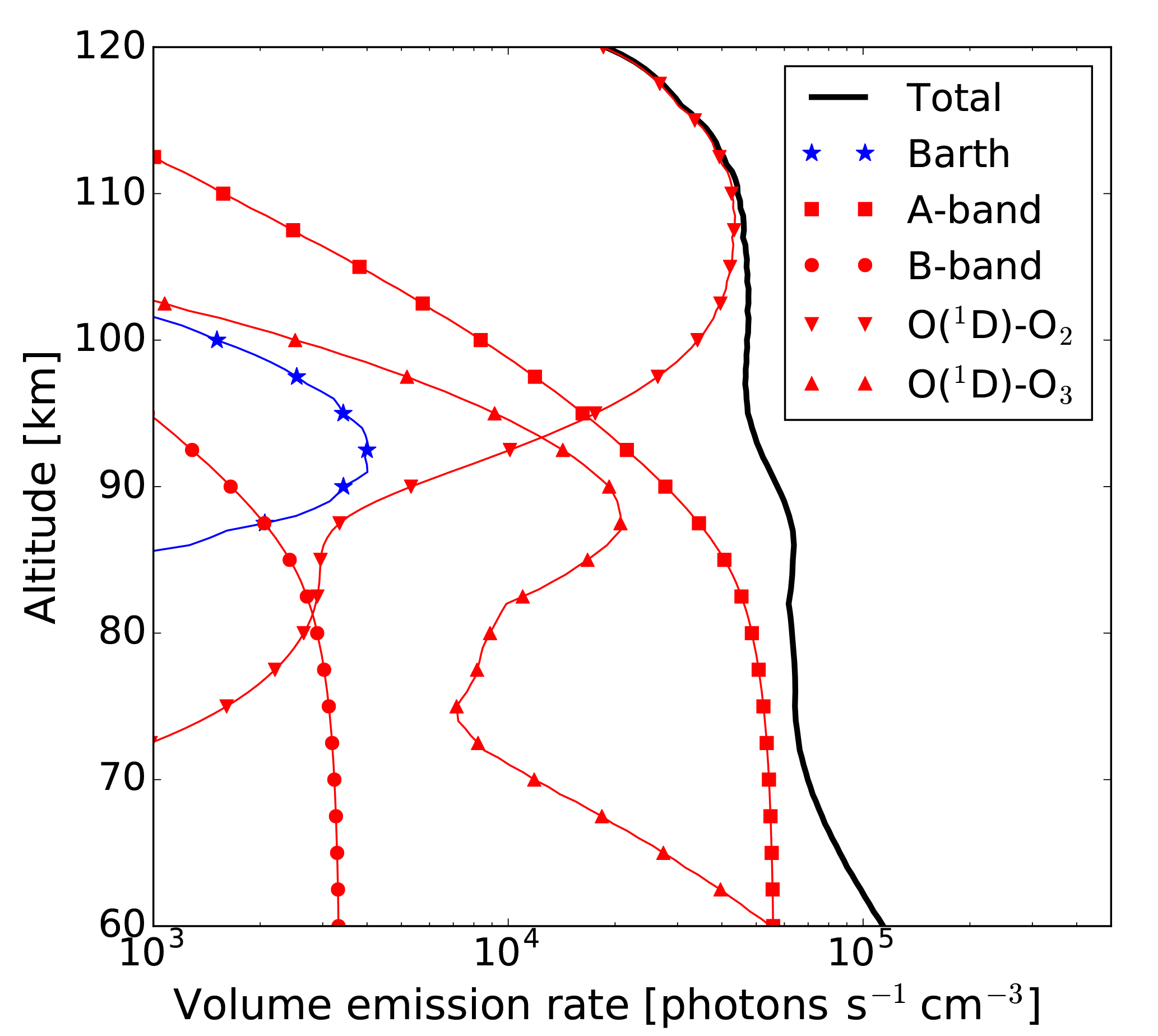
Figure 1Volume emission rate of O₂($b^{\mathrm{1}}{\mathrm{\Sigma }}_g^{+}$) separated by excitation processes. “Barth” indicates the emission rates created by the recombination of atomic oxygen. This is the only excitation process being active during day and night. “A-band” and “B-band” label the fraction of emissions excited by resonance absorption in those bands. “O₂” and “O₃” mark the excitation by collisions with O(¹D), which is created by photolysis of O₂ and O₃, respectively.

Download

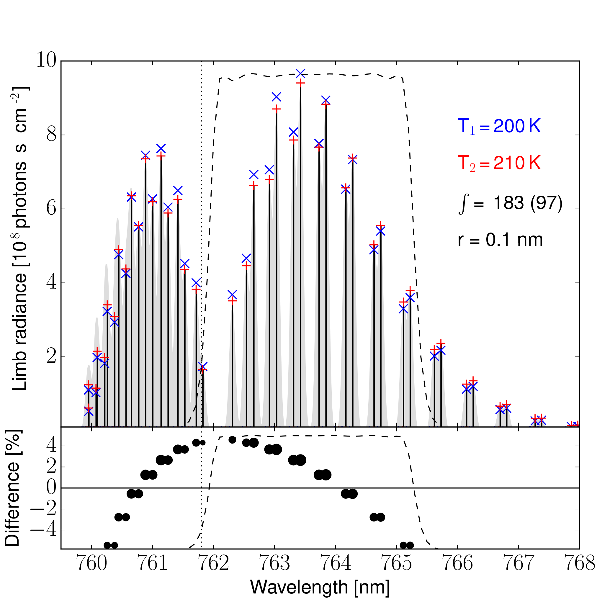
Figure 2O₂ A-band limb emission line calculations assuming a global temperature of 200 and 210 K (upper panel). The spectra in the upper panel have been normalized to show identical band intensities. The vertical bars and the blue signs mark the emission line intensities for 200 K; the light gray area shows their intensities (multiplied by a factor of 10) as seen from an instrument with a spectral resolution of 0.1 nm. The red + signs show line intensities for 210 K. The dashed line is the filter transmission curve of the instrument presented later. The dotted vertical line is drawn at the Littrow wavelength. Within the filter, more than 50 % of the total band intensity (at 200 K) are emitted (97 out of 183 photons s⁻¹ cm⁻² sr⁻¹). The percentage difference of the line intensities at 200 and 210 K is shown in the lower panel; the symbol size scales with the absolute intensity of the lines. The atmospheric background data are taken from the HAMMONIA model, and the spectroscopic data stem from the HITRAN database (Gordon et al., 2017).

Download

At the beginning of this project, different instrument concepts were considered to detect the mesospheric A-band limb emissions from a CubeSat (Deiml et al., 2014). For a variety of reasons, we decided to develop the instrument with a spectrometer. Performance considerations lead to the selection of a Fourier transform spectrometer (FTS). With its compact and monolithic design (Shepherd et al., 2016), a spatial heterodyne spectrometer (SHS) deemed the most appropriate candidate, in accordance with the findings of Watchorn et al. (2014) in the framework of another study.

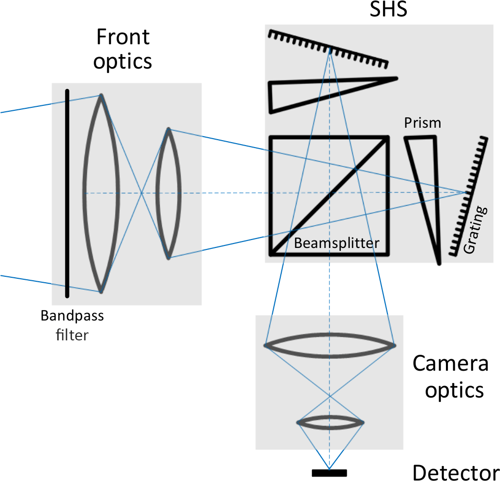
In principle, a SHS is a FTS, where the mirrors in each arm are replaced by diffraction gratings (Fig. 3). The incoming wavefront is diffracted at the gratings, with a wavelength-dependent angle. The superposition of the two wavefronts then produces straight, parallel, and equidistant fringes with a spatial frequency depending on the wavelength of the light. The zero frequency of the fringe pattern is at the Littrow wavelength and small wave number changes result in fringes with a discernable spatial frequency, which can be observed with available imaging detectors. The concept was originally proposed by Pierre Connes in a configuration called Spectromètre interférential à selection par l'amplitude de modulation (SISAM) (Connes, 1958). With the advent of imaging detectors, this idea was taken up by Harlander and Roesler (1990), Douglas (1997), Smith and Harlander (1999), Watchorn et al. (2001), Harris et al. (2004), Roesler (2007), Englert et al. (2010), Watchorn et al. (2010), Bourassa et al. (2016), and Lenzner and Diels (2016), among others. The design of a SHS for a particular wavelength and spectral resolution follows a few simple relations, which are shortly summarized to illustrate the main characteristics of this device. For a derivation of the mathematical expressions see, e.g. Harlander (1991), Cooke et al. (1999), Smith and Harlander (1999), and references cited therein.

The tilt angle of the gratings with respect to the optical axis is called Littrow angle Θ_L. Light at the Littrow wave number σ_L is returned in the same direction as the incoming path, as described by the grating equation (for diffraction order 1 and grating groove density 1∕d):

Figure 3Basic design of the SHS with front and detector optics.

Download

Combining the intensity equation of a conventional FTS and the grating equation for small incident angles at the grating gives the SHS equation for ideal conditions, relating the incoming radiation S at wave number σ to the spectral density I at position x, parallel to the dispersion plane:

κ is the heterodyned fringe frequency:

The maximum resolving power R of a SHS is nearly proportional to the number of grating grooves illuminated by the incoming beam or in other words the illuminated spot size W on the grating multiplied by the grating groove density g times 2:

The bandpass of a SHS is limited by the detector resolution due to the Nyquist theorem. This means that the spectral range ${\mathit{\lambda }}_{max}-{\mathit{\lambda }}_{min}$, which can be detected for given spectral resolution Δλ, has to be lower than half the pixel number N:

As for conventional FTS or Fabry–Pérot instruments, the acceptance angle of light for a conventional SHS is inversely proportional to its resolving power R (Harlander, 1991), which is a few orders of magnitude larger than for conventional grating spectrometers of the same size. The acceptance angle of a SHS can be increased significantly when prisms are inserted into the two interferometer arms. This configuration was first implemented for upper-atmospheric temperature measurements by Hilliard and Shepherd (1966) with a Michelson interferometer and first introduced for a SHS by Roesler and Harlander (1990). The prisms incline the image of the gratings so that they appear to be located in a common virtual plane which is oriented perpendicular to the optical axis for a wide range of incident angles. At the end, the acceptance angle of the SHS, including field widening prisms, is only limited by spherical aberration for systems with small Littrow angles and astigmatism for large Littrow angles (Harlander et al., 1992). Depending on the actual design, the prisms increase the etendue or throughput of a SHS by 1–2 orders of magnitude. The calculation of the prism apex angle is given by, for example, Harlander et al. (1992).

A general advantage of SHS is the relaxed alignment tolerances, because in most optical setups the gratings are imaged onto a focal plane array. As a result, each detector pixel sees only a small area of the optical elements, so that moderate misalignments or inaccuracies in the surface quality affect limited spatial regions on the detector only. This means that the interferogram is distorted locally rather than reduced in contrast. The main benefit of the SHS is that they can be built monolithically, making them very robust for harsh environments, e.g. during rocket launches.

The basic design parameters of the SHS were calculated analytically using the SHS equations mentioned above. The materials of the optical glass components, the apex angle of the prisms, and the distances between the various components were optimized and iterated by means of optical ray tracing software (ZEMAX). The resulting basic design parameters are summarized in Table 1. A simulated interferogram of the O₂ A-band as seen from this instrument is illustrated in Fig. 4.

Table 1Summary of optics and filter properties.

Download Print Version | Download XLSX

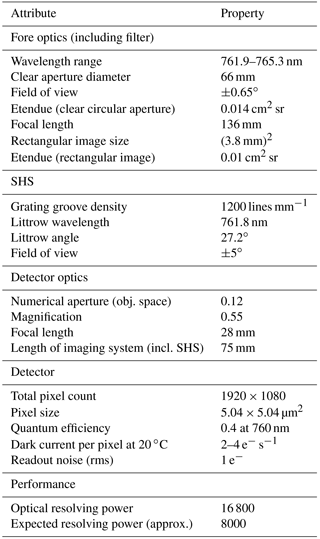
An integral part of a SHS design is the optical filter located between the SHS and the scene to be observed. For this instrument, a six-cavity design bandpass filter with a centre wavelength of 763.6 nm and a bandwidth of 3.3 nm was chosen. The filter is illuminated at an angle of incidence of ±0.65^∘, resulting in a blue shift of 0.8 nm. The temperature coefficient of this filter is 5 pm K⁻¹, resulting in a spectral shift of the bandpass of 0.3 nm between −10 and +50^∘.

Since a SHS instrument maps the spectrum on both sides of the Littrow wavelength symmetrically into Fourier space, the filter must be adapted in such a way that there is no overlap of lines from different sides of the Littrow wavelength in the interferogram. In our design, the Littrow wavelength is at 761.8 nm; i.e. the filter blocks most of the radiance from the shorter wavelength side of the Littrow wavelength (Fig. 2).

The purpose of the front optics is to image a scene at the Earth's limb onto the gratings. The detector optics images the gratings onto the focal plane of the 2-D detector. The image at the detector contains spatial information about the scene in both dimensions. An interferogram is superimposed on this scene in the direction perpendicular to the grating grooves. For the instrument presented in this work, the gratings are oriented in such a way that the interferogram spans over the horizontal direction, assuming that intensity fluctuations in the horizontal direction are small or smeared out during the exposure of the image compared to the modulation depth of the interferogram, which is valid in atmospheric limb sounding. The front optics (Fig. 5) consists of four lenses, which image an object at infinity onto a square with an edge length of 7 mm on the virtual image of the gratings. This corresponds to a theoretical spectral resolution of about 16 800 (Eq. 4). The maximum chief ray angle extent is about 1.9^∘, such that a rectangular object with an angular extent of 1.3^∘ can be captured without vignetting. The clear aperture diameter of the front lens is 66 mm and the distance between the first lens and the SHS is 104 mm. The etendue of this configuration is 0.014 cm² sr for the clear circular aperture and 0.01 cm² sr for the rectangle mentioned above.

Figure 4Simulated interferogram of the O₂ A-band nighttime emission for various altitudes.

Download

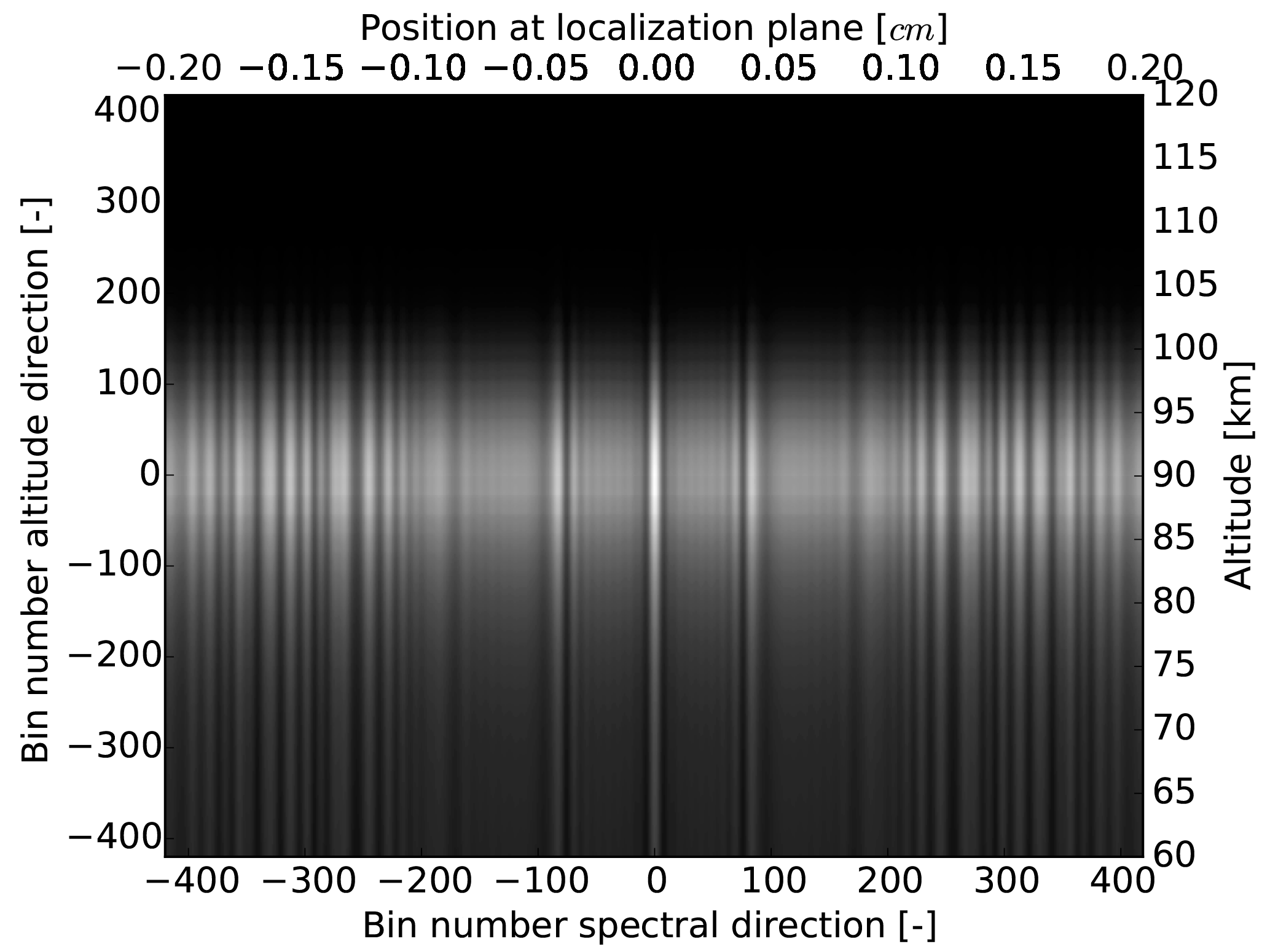
Figure 5Optical components of the instrument, including the interference filter, the front optics, the SHS, the detector optics, and the detector.

Download

The detector optics images the active area of the gratings onto the detector and consists of lenses as well. The magnification is 0.55; i.e. the illuminated area at the detector has a diameter of about 3.8 mm. This value was chosen as a trade-off between the form factor required and the desired spectral and spatial resolution (see below). The distance between the beam splitter and the detector focal plane is 46 mm.

The aperture stop of the optical system, which limits the amount of light passing through the instrument, is the mounting of the first lens of the front optics. In the current version of the instrument, there is a Lyot stop after the last lens of the detector optics.

Figure 6Simulated interferogram for a focused configuration considering wave aberrations.

Download

The detector chosen for this instrument is a low noise silicon-based CMOS image sensor from Fairchild Imaging (HWK1910A). The optical format is 2∕3 (9.7 mm × 5.4 mm) and the pixel size is 5 µm × 5 µm, resulting in 1920 × 1080 pixels in total; from those 760 × 760 pixels are needed to capture a rectangular image of 3.8 mm². The quantum efficiency of the detector at 762 nm is about 0.4.

Like the SHS, the entire optical system was optimized using optical ray tracing software as well. The wavefront peak-to-valley extension of the optical system is less than a half wavelength for centre rays and one wavelength at maximum for the edge region of the field. The extension of the point spread function is 5 µm for inner and 10 µm for outer pixels, which does not deteriorate the determination of the different waves in the interferogram, because the highest spatial frequency to be observed has a wavelength of about 45 µm. Optical distortions introduced in the common optical path are not part of the optimization procedure, because they can be removed in the post-processing or calibration of the instrument.

To evaluate the spectrometric performance of the system, the differences in the phase distortion of the two arms are most relevant, because this would result in an irreversible loss of contrast. This quantity is not directly accessible by the figures of merit mentioned above. This effect was investigated by calculating the wave aberrations in the exit pupil of the system for object and reference arm, respectively. The corresponding complex amplitudes are then superposed and propagated into the detector plane by a Fourier transformation. Taking the absolute square of the resulting amplitude gives the intensity distribution for the corresponding light source point (Fig. 6). The detection plane was placed between the focal planes for the on-axis and the 0.65^∘ off-axis light source points as a compromise and closer to the latter to enhance the visibility on the edges of the interferogram. Nevertheless, the visibility reduction is about one-third towards the edges. Interestingly, the highest visibility is achieved by placing the detector plane outside both focal planes in a plane which is near the on-axis focal point. The suspected reason is that the shape of the focal spots, which are blurred by aberrations resulting in a reduction of visibility, becomes more compact if the detector plane is positioned slightly out of the on-axis focus, yielding to higher contrast (Fig. 7). The SHS has a fairly athermal design, but the foci and the modulation transfer function (MTF) of the entire optical system depend more on temperature. For low spatial frequencies this effect is small, but for the highest spatial frequencies seen by the instrument the MTF reduces from about 85 % at 20 ^∘C to about 70 % at 0 ^∘C. Further simulations and comparison with measurements are in preparation.

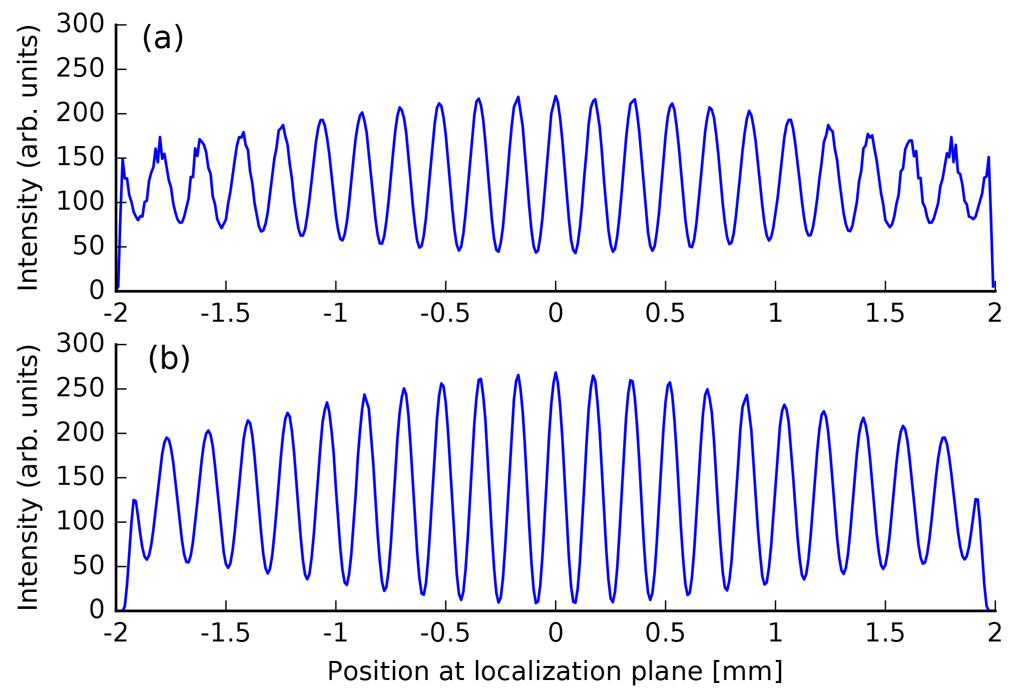
Figure 7Simulated interferograms for the centre row of the 2-D interferogram (Fig. 6). The upper plot shows the interferogram at the Gaussian focal point and the lower one at a slightly shifted position, where the foci across the image considering wave aberrations are more compact than at the Gaussian focus.

Download

To determine the expected signal-to-noise ratio of the instrument for a given integration time, we estimate the amount of incoming light that is available in the modulated part of the interferogram and the noise of the detector. In a SHS, 50 % of the incoming radiation are lost at the beam splitter. The holographic gratings used have an efficiency of about two-third at 765 nm, so that another one-third of the radiation is not available in the modulated part of the radiance. Misalignments and aberrations of optical components are estimated to reduce the contrast of the interferogram, so that we expect to detect about 20 % in the modulated part of the interferogram.

The limb radiances of a strong line in the O₂ A-band nightglow maximum recorded over an altitude range of 1.5 km are about 1×10⁹ photons s⁻¹ cm⁻² sr⁻¹ (cf. Fig. 2). Considering the etendue of the system and the fraction of the detector illuminated by this emission layer (about 2 %), and assuming that 20 % of the photons end up in the modulated part of the signal, this yields to about 50 photons s⁻¹ at every pixel recording the interferogram. Since the intensities from a vertical layer of 1.5 km thickness illuminate 20 detector rows, the average signal introduced by one emission line on an individual detector pixel is 3 photons s⁻¹. Considering that the detector records light from all spectral elements within the bandpass of the instrument, and some radiance will end up in the unmodulated part of the interferogram, each detector pixel will record about 40 photons s⁻¹.

The noise of the signal is, by far, limited by shot noise, which scales with the square root of the (electrical) signal. The latter consists of the electrons excited by the signal of interest and the dark current caused by thermal processes. According to our own measurements, the dark current of the detector is 2–4 e⁻ s⁻¹ pixel⁻¹ (corresponding to a photon flux of 5–10 photons/s/pixel) at 20 ^∘C, which is a factor of 7–10 lower than the threshold given by the manufacturer. The dark current decreases a factor of 2 every 7 K (Liu et al., 2018).

At 20 ^∘C, the dark current is at least a factor of 5 lower than the atmospheric signal in the emission layer maximum and therefore not a dominant source of random noise at these altitudes. This becomes more critical at other altitudes and for higher detector temperatures. Therefore the detector should be operated below 20 ^∘C. The readout noise of the detector was measured to 1 e⁻, which is in agreement with the specification given by the manufacturer. Taking into account that 20 detector rows are summed up for each altitude bin, this noise component is negligible for integration times larger than 1 s compared to the shot noise.

The required signal-to-noise ratio to achieve a given temperature precision was determined by Monte Carlo simulations: first, a simulated spectrum with the optical resolving power of 16 800 was calculated. This spectrum was inverse Fourier-transformed and white noise was added. In the next step, the spectral power in the various frequencies was estimated by applying a Fourier transformation using a windowing function. The resulting spectra were then used to retrieve an atmospheric temperature profile and some other instrumental parameters, such as the spectral resolution of the data. Considering the intensity of the A-band signal of the nightglow layer maximum and the detector performance, the expected signal-to-noise ratio for a vertical resolution of 1.5 km and an integration time of 60 s will be 10–20 in the nightglow maximum, resulting in a retrieved temperature precision of 1–2 K.

The conversion of the detector signal into calibrated spectra involves a number of calibration steps. As pointed out in the previous section, the modulated to unmodulated signal ratio is one of the key points here. To quantify this ratio, the SHS equation for idealized conditions (Eq. 2) has to be extended (Englert and Harlander, 2006):

For better clarity, the integration variable in these expression is the heterodyned fringe frequency κ instead of wave number σ, which is a normal linear dependency. One of the extensions compared to Eq. (2) is the introduction of different intensity transmission functions t_A and t_B for the two SHS arms. In addition, a term ϵ(x,κ) was added, which considers that the modulation efficiency can depend on the location within the interferogram and its frequency. Finally, a phase distortion term Δ(x,κ) quantifying any phase and frequency distortions within the interferogram was introduced.

Before the interferograms of the instrument are analysed, barrel or pincushion distortions of the image are corrected because they affect the distribution of spatial information and modify the frequency of the interferogram at the same time. Due to the highly compact design of the optics and the use of spherical lenses only, significant image distortions are expected. To characterize image distortions of the entire optical system, a line grid target will be positioned in front of the instrument. Then, the SHS arms are blocked one by one to record two images of the test target. The division model (Fitzgibbon, 2001) will be used to correct for the spherical symmetric distortions. Within this model, radial distortion coefficients are fitted to straighten lines in the image. These measurements will also verify the geometrical point spread functions, which are expected to be much smaller than the required spatial resolution of the instrument.

According to computer simulations, about 90 % of the image distortions are introduced by the detector optics. Therefore it is also possible to verify and to monitor the image distortions using interferograms. Here, the reference image is generated from an interferogram by an adaptive edge detection algorithm. The edges correspond in a sense to the reference lines of a test image. It is expected that image distortions affect interferograms with different spatial frequencies in the same way.

To characterize and quantify the modulated part of the intensity, an optical setup with a tunable laser is used. First, the laser light is homogenized using microlens arrays and imaged onto a rotating diffusor. The laser spot on the diffusor is set to infinity by a large lens, such that the full aperture of the instrument is uniformly illuminated by plane waves with a divergence of at least ±0.65^∘. The laser frequency and power are continuously monitored during the measurement. The laser power and the flux are calibrated before the measurements are taken.

The first step in the analysis of these measurements is to fit a frequency-dependent polynomial correction of the phase depending on the position in the localization plane. Depending on the real instrument performance, the usage of a lookup table is another option to homogenize the phase across the interferograms.

Next, the modulated part of the signal is quantified by looking at a quantity called visibility ν, which is defined as the amplitude of the modulation normalized to the average signal (times 2):

The visibility depends on several factors, such as internal stray light, the grating performance, surface or material properties or imperfections, misalignments, and contamination. Visibility depends on the MTF and can be frequency dependent. It can also vary across the field as a consequence of strong aberrations or misalignments of the system. Since the total power for each spectral element is needed for temperature retrieval, the visibility calibration is as important as a radiometric calibration, and it can even cover the radiometric calibration if the power of the laser scene is known well enough. To get the modulation or envelope function of the monochromatic interferogram as needed for the visibility calibration, we calculate its Hilbert transform, which is fundamentally the same idea as the methods described in Englert et al. (2004) and Englert and Harlander (2006), where the corresponding complex or imaginary interferogram is generated from the real interferogram. The sum of the signal and its Hilbert transform as imaginary part gives an analytic or holomorphic representation of the interferogram (Feldman, 2011). The absolute value of this complex-valued signal gives the instantaneous amplitude or envelope of the signal.

In theory and for ideal conditions, the visibility characterization covers an additional calibration step called “flat fielding” that corrects for non-uniformities caused by different sensitivities of detector elements, inhomogeneities within optical components, or any kind of misalignment of the optical components including the SHS. Englert and Harlander (2006) give an overview about different flat-fielding approaches. To verify the uniformity of the calibrated signal, we plan to perform the “balanced arm flat-fielding approach”, where the entire instrument is illuminated by our laser-driven optical setup or any other uniform radiation source and one by one SHS arm is blocked. In this case, the measured radiation corresponds to the “non-modulated” intensity term.

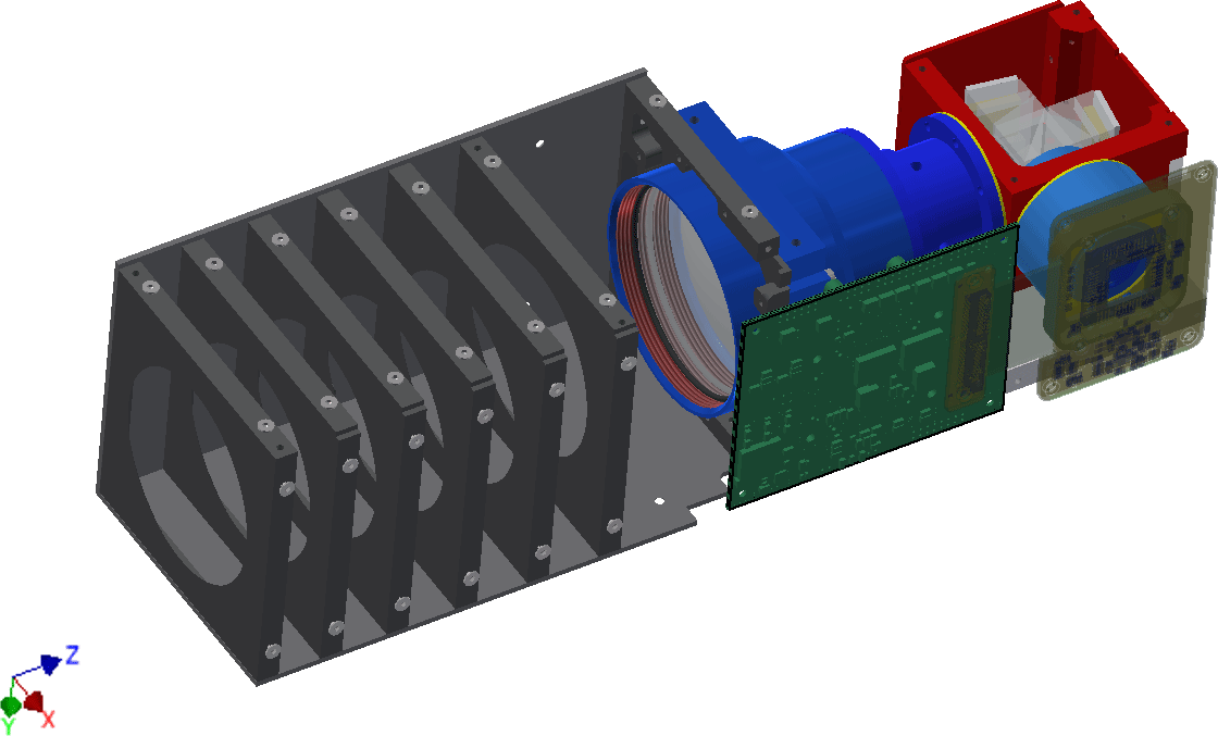
Figure 8Design image of the instrument. The total length is 30 cm and the front face about 10 × 10 cm².

Download

Design data can be found directly throughout the text and in Table 1.

The authors declare that they have no conflict of interest.