the Creative Commons Attribution 4.0 License.
the Creative Commons Attribution 4.0 License.
 | 25 Jul 2018
The SPARC water vapour assessment II: comparison of stratospheric and lower mesospheric water vapour time series observed from satellites
Farahnaz Khosrawi
Stefan Lossow
Gabriele P. Stiller
Karen H. Rosenlof
Joachim Urban
John P. Burrows
Robert P. Damadeo
Patrick Eriksson
Maya García-Comas
John C. Gille
Yasuko Kasai
Michael Kiefer
Gerald E. Nedoluha
Stefan Noël
Piera Raspollini
William G. Read
Alexei Rozanov
Christopher E. Sioris
Kaley A. Walker
Katja Weigel
Time series of stratospheric and lower mesospheric water vapour using 33 data sets from 15 different satellite instruments were compared in the framework of the second SPARC (Stratosphere-troposphere Processes And their Role in Climate) water vapour assessment (WAVAS-II). This comparison aimed to provide a comprehensive overview of the typical uncertainties in the observational database that can be considered in the future in observational and modelling studies, e.g addressing stratospheric water vapour trends. The time series comparisons are presented for the three latitude bands, the Antarctic (80∘–70∘ S), the tropics (15∘ S–15∘ N) and the Northern Hemisphere mid-latitudes (50∘–60∘ N) at four different altitudes (0.1, 3, 10 and 80 hPa) covering the stratosphere and lower mesosphere. The combined temporal coverage of observations from the 15 satellite instruments allowed the consideration of the time period 1986–2014. In addition to the qualitative comparison of the time series, the agreement of the data sets is assessed quantitatively in the form of the spread (i.e. the difference between the maximum and minimum volume mixing ratios among the data sets), the (Pearson) correlation coefficient and the drift (i.e. linear changes of the difference between time series over time). Generally, good agreement between the time series was found in the middle stratosphere while larger differences were found in the lower mesosphere and near the tropopause. Concerning the latitude bands, the largest differences were found in the Antarctic while the best agreement was found for the tropics. From our assessment we find that most data sets can be considered in future observational and modelling studies, e.g. addressing stratospheric and lower mesospheric water vapour variability and trends, if data set specific characteristics (e.g. drift) and restrictions (e.g. temporal and spatial coverage) are taken into account.
- Article
(8713 KB) -
Supplement
(11643 KB) - BibTeX
- EndNote


We would like to dedicate this paper to our highly valued colleague Jo Urban, who would have certainly been the lead author of this study had he not passed away so soon. Without his devoted work on UTLS water vapour over many years, this work would not have been possible. In particular, the retrieval of water vapour from the SMR observations and the combination of these data with other data sets to understand the long-term development of this trace constituent comprised a large part his life's work. With his passing, we lost not only a treasured colleague and friend, but also a leading expert in the microwave and sub-millimetre observation community.
Water vapour is the most important greenhouse gas and plays a key role in the chemistry and radiative balance of the atmosphere. Any changes in atmospheric water vapour have important implications for the global climate (Riese et al., 2012; Solomon et al., 2010) and need to be monitored and understood (Müller et al., 2016). Accurate knowledge of the water vapour distribution and its trends from the upper troposphere up to the mesosphere is therefore crucial for understanding climate change and chemical forcing (Hegglin et al., 2013).
Water vapour is the source of the hydroxyl radical (OH) which controls the lifetime of shorter-lived pollutants, tropospheric and stratospheric ozone and other longer-lived greenhouse gases such as methane (Seinfeld and Pandis, 2006). Further, water vapour is an essential component of polar stratospheric clouds (PSCs) which play a key role in Antarctic and Arctic ozone depletion during winter and spring (Solomon, 1999). Accordingly, water vapour has an important influence on stratospheric chemistry through its ability to form ice particles. Dehydration, that is, the removal of water vapour from the gas phase, can either be a reversible or an irreversible process depending on the lifetime of water-containing particles and their size. However, ice particles generally live long enough and grow sufficiently large to fall and remove water vapour permanently from an air mass so that dehydration can generally be defined as an irreversible process. Dehydration in the stratosphere is generally observed over the Antarctic during winter (Kelly et al., 1989; Nedoluha et al., 2000, 2007; Vömel et al., 1995) and to a lesser extent also over the Arctic (Fahey et al., 1990; Khaykin et al., 2013; Manney and Lawrence, 2016; Pan et al., 2002) as well as at the tropical tropopause (Jensen et al., 1996; Read et al., 2004; Schiller et al., 2009).
In addition to its role in the Earth's radiative budget and middle atmospheric chemistry, water vapour is an important tracer for transport in the stratosphere and lower mesosphere. Dynamical circulations that can be diagnosed with water vapour in the middle atmosphere are the Brewer–Dobson circulation in the stratosphere and the pole-to-pole circulation in the mesosphere (Brewer, 1949; Lossow et al., 2017a; Mote et al., 1996; Pumphrey and Harwood, 1997; Remsberg et al., 1984, 2018; Seele and Hartogh, 1999). In the stratosphere, the water vapour abundance is primarily governed by two main sources: (1) the transport from the troposphere through the tropical tropopause layer (TTL), where the minimum temperature (the so-called cold point temperature) determines how much water vapour enters the stratosphere (Fueglistaler and Haynes, 2005); (2) the oxidation of methane, which is the only important chemical source of water vapour in the stratosphere (Bates and Nicolet, 1950; Le Texier et al., 1988).
A major research focus in relation to water vapour has been on the detection and attribution of long-term changes in stratospheric and mesospheric water vapour based on in situ and remote sensing measurements (Dessler et al., 2014; Hegglin et al., 2014; Hurst et al., 2011; Nedoluha et al., 2003; Oltmans and Hofmann, 1995; Oltmans et al., 2000; Rosenlof et al., 2001; Scherer et al., 2008). Many of these measurements have indicated an increase in stratospheric and mesospheric water vapour that has significant implications for atmospheric temperature. Increases in stratospheric water vapour cool the stratosphere but warm the troposphere (Solomon et al., 2010). Model simulations predict a ∼1 K decrease in stratospheric temperature per decade along with a 0.5–1 ppmv increase of water vapour in the 21st century (Gettelman et al., 2010). Both the future cooling of the stratosphere and the future increase in water vapour enhance the potential for the formation of PSCs, which would have significant implications on Arctic and Antarctic dehydration and ozone loss (Khosrawi et al., 2016; Thölix et al., 2016). The methane increase in the stratosphere can only explain part of the observed water vapour changes (Hurst et al., 2011; Rosenlof et al., 2001). A complete understanding of water vapour changes also requires good knowledge of short-term variability, such as the annual oscillation (AO) and semi-annual oscillation (SAO) or the variations caused by the quasi-biennial oscillation (Kawatani et al., 2014; Lossow et al., 2017b; Remsberg, 2010; Schoeberl et al., 2008).
In addition to an observed long-term increase in stratospheric water vapour, pronounced drops have occasionally been observed. One drop (sometimes denoted as the millennium drop) occurred in 2000 (Brinkop et al., 2016; Randel et al., 2006; Scherer et al., 2008; Solomon et al., 2010; Urban et al., 2012), with water vapour abundances starting to recover around 2004–2005 onwards. This decrease was caused by a reduced transport of water vapour across the tropical tropopause in response to lower cold point temperatures. The exact driving mechanism is still in question, but has been suggested to be due to variations of the QBO (quasi-biennial oscillation), ENSO (El Niño Southern Oscillation) and the Brewer–Dobson circulation that collectively acted in the same direction lowering the tropopause temperatures. In 2011 and 2012 another drop occurred, which however was shorter-lived than the millennium drop (Urban et al., 2014). Recently, another sharp decrease was observed in connection with the QBO disruption and the unusual El Niño event in 2015 and 2016 (Avery et al., 2017; Tweedy et al., 2017), but this decrease has also already recovered.
Within the framework of the second SPARC water vapour assessment (WAVAS-II), we compared time series of stratospheric and lower mesospheric water vapour derived from a number of different satellite data sets. The time series comparison was performed for the Antarctic (80∘–70∘ S), the tropics (15∘ S–15∘ N) and the Northern Hemisphere mid-latitudes (50∘–60∘ N) at four different altitudes (0.1, 3, 10 and 80 hPa). This selection of latitude bands covers all three basic climatic regions (i.e. tropics, mid-latitudes and polar region) and allows the inclusion of all stratospheric WAVAS-II data sets in the comparison. The combined temporal coverage of the 15 satellite instruments allows the consideration of the time period 1986–2014. This work aims to provide estimates of the typical uncertainties in the time series from satellite observations that should be taken into account in observational and modelling studies. A brief overview of the data sets used in this study is provided in the next section followed by a description of the analysis approach in Sect. 4. In Sect. 5 the results are presented, focusing on the comparison of the de-seasonalised water vapour time series. Comparison results for the absolute time series are given in the Supplement. Finally, our results will be summarised and conclusions will be given in Sect. 6.
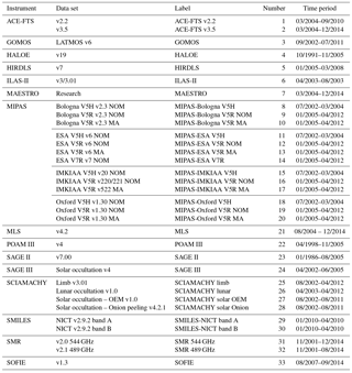
For the comparison of water vapour products performed within the second SPARC WAVAS-II assessment, 40 data sets (not including data sets of minor water vapour isotopologues) have been considered, primarily focusing on the time period from 2000 to 2014 (Walker and Stiller, 2018). In the present study, we included all 33 data sets that have observational coverage in the stratosphere. A list of these data sets is provided in Table 1, along with the effective time periods available for analysis. In addition, this table provides the data set labels and numbers used in the figures. Overall, data sets from the following 15 instruments have been considered (listed in alphabetical order): ACE-FTS, GOMOS, HALOE, HIRDLS, ILAS-II, MAESTRO, MIPAS, MLS (aboard the Aura satellite, not the instrument on the Upper Atmosphere Research Satellite – UARS), POAM III, SAGE II, SAGE III, SCIAMACHY, SMILES, SMR and SOFIE. For a number of instruments there are multiple data sets based on different data processors, measurement geometries, retrieval versions and spectral signatures used to derive the water vapour information. This especially holds for MIPAS, where 13 data sets have been included in this comparison. The MIPAS measurements are processed by four different processing centres: (1) the University of Bologna (Dinelli et al., 2010), (2) the European Space Agency (ESA; Raspollini et al., 2013), (3) IMK/IAA (Stiller et al., 2012a; von Clarmann et al., 2009) and (4) Oxford (Payne et al., 2007). The four processors differ in several respects, such as their choices of spectral ranges (so called micro-windows), the vertical grid on which the retrievals are performed (pressure or geometric altitude), the choice of regularisation (and related to this, the vertical resolution), the choice of spectroscopic database, the sophistication of the radiative transfer (in particular, whether or not non-local thermodynamic equilibrium, NLTE, emissions are considered) and whether or not any attempt is made to account for horizontal inhomogeneities, and the a priori and the assumed p–T profile. Indeed, the temperature used might be a large source of error for species retrieved in LTE regions. Some of the different processing schemes also make use of different level-1b data versions (here V5 and V7) based on different ESA calibrations. The spread of results seen for MIPAS indicates how specific choices within a retrieval approach may influence the retrieval results. The HALOE, POAM III and SAGE II data sets also include observations before 2000. These were considered in the comparisons, so that the combined temporal coverage of all data sets ranges from 1986 to 2014. A complete description of the data sets and their characteristics can be found in the WAVAS-II data set overview paper by Walker and Stiller (2018). In comparison to our previous SPARC WAVAS-II paper (Lossow et al., 2017b) the following two data related changes have been made: (1) the ACE-FTS v3.5 and MAESTRO data sets have been extended from March 2013 until December 2014 (see Table 1 of Lossow et al., 2017b). (2) The MIPAS ESA v7 data set has been completed. In the aforementioned study, this data set comprised only a sample of 200 000 observations (instead of 1 800 000), though at the time the temporal coverage on a monthly basis had already been completed.
Table 1Overview over the water vapour data sets from satellites used in this study.
3.1 Time series calculation
For the first step, we screened the individual data sets according to the criteria recommended by the data providers. A complete list of these criteria is given in the WAVAS-II data set overview paper by Walker and Stiller (2018). After the screening we interpolated the data onto a regular pressure grid. This comprises 32 levels per pressure decade, which corresponds to a fine vertical sampling of about 0.5 km. The uppermost level we consider is 0.1 hPa. The interpolated profiles were then binned monthly and for the three latitude bands chosen: 80∘–70∘ S, 15∘ S–15∘ N and 50∘–60∘ N. The monthly zonal means are given as
In the equation above describes the individual observations that fall into a given time t (i.e. month) and latitude ϕ bin, indicates their total number and z denotes the altitude level. Before this calculation the data in the given bin were screened using the median and the median absolute difference (MAD, Jones et al., 2012) in an attempt to remove unrepresentative observations that occasionally occur. Data points outside the interval 〈median[ MAD[]〉, with …, were discarded, targeting the most prominent outliers (Jones et al., 2012; Lossow et al., 2017b). For a normally distributed data set, 7.5 MAD corresponds to about 5σ. For individual data sets this concerned on average between 0.03 % and 3.2 % percent of the data in a given bin. Averaged over all data sets typically 0.6 % of the data in a given bin were removed by this screening. In addition to the monthly zonal means, the corresponding standard error was calculated by
To avoid spurious data, averages that are smaller than their corresponding standard errors in an absolute scale were discarded. Also, monthly averages based on less than 20 observations for dense data sets (e.g. HIRDLS, MIPAS, MLS, SCIAMACHY limb, SMILES-NICT and SMR) and less than 5 observations for sparse data sets (e.g. ACE-FTS, GOMOS, HALOE, ILAS-II, MAESTRO, POAM III, SAGE II, SAGE III, SCIAMACHY occultation and SOFIE) were not considered any further. This is a slightly more relaxed approach than used in the time series analysis by Lossow et al. (2017b), where a minimum of 20 observations was required for all data sets. However, additional tests have shown that such a conservative criterion is not required for the sparser data sets.
In our analysis we consider both absolute time series and de-seasonalised time series. The ILAS-II and SMILES data sets cover less than one year, so that a de-seasonalisation is not meaningful. There are multiple ways to achieve a de-seasonalisation. The most common and simplest approach is to calculate for a given calendar month the average over several years. Subsequently this average is subtracted from the individual months contributing to this climatological average (i.e. average approach). This approach requires that a data set covers every calendar month at least twice. For the MIPAS V5H data sets this requirement is not fulfilled as they cover only 21 months. To accomplish a de-seasonalisation even for these data sets a regression approach was used. Every data set was regressed with the following regression model:
This model contained an offset as well as the annual oscillation (AO) and semi-annual oscillation (SAO). The AO and SAO are parameterised by orthogonal sine and cosine functions. denotes the fit of the regressed time series and C are the regression coefficients of the individual model components. pAO=1 year is the period of the annual oscillation; likewise pSAO=0.5 years is the period of the semi-annual oscillation. In accordance to pAO and pSAO given in years, the time t is here also used on a yearly scale. To calculate the regression coefficients we followed the method outlined by von Clarmann et al. (2010) using the standard errors (their inverse squared) of the monthly zonal means as statistical weights. Autocorrelation effects and empirical errors (Stiller et al., 2012b) were not considered in this regression. The de-seasonalised time series , thus the anomalies for each time t, are then given as
For the sake of simplicity we do not assign any error to the regression fit, so that the standard error of the de-seasonalised time series is given by
3.2 Comparison parameters
To assess how the different time series compare between two data sets or altogether we use a number of parameters, namely the spread (i.e. the difference between the maximum and minimum volume mixing ratios among the data sets), the (Pearson) correlation coefficient and the drift (i.e. linear changes of the difference between time series over time). In the following subsections, the calculation of these parameters is described in more detail.
3.2.1 Spread
We define the spread as the difference between the maximum and minimum volume mixing ratio among the data sets at a given time and place. As such, the spread is a simple measure of the collective consistency among the time series from the different data sets. We have chosen this approach for the spread calculation since for the other approaches based on standard deviation or percentiles, assumptions have to be made. However, we have also calculated the spread using the other two approaches and derived qualitatively the same results as for the maximum–minimum calculation. Prior to the spread calculation, we performed an additional screening among the data sets to avoid unrepresentative spread estimates. The screening is again based on the median and median absolute difference, as done before for the monthly zonal mean calculation. Monthly zonal means outside the interval 〈median[ MAD[]〉 were not considered, with and denoting the number of data sets at a given time, latitude and altitude. The subscript p is used as a placeholder either for the absolute or the de-seasonalised data. This screening removed overall 2.6 % of the data for the latitude band between 80∘ and 70∘ S. For the tropical and the mid-latitude bands, respectively 3.6 % and 3.7 % of the data were removed. Subsequently, the spread was derived. We did not impose any additional criterion on the number of data sets available for a spread estimate to be valid (two data sets is the natural minimum). However, for much of the 1990s the only available satellite data sets are HALOE and SAGE II. Since both instruments provide solar occultation measurements, the number of coincidences is limited. Thus, their time series do not constantly overlap, there are many gaps in the spread. Therefore, we focus in the results section on the time period between 2000 and 2014.
3.2.2 Correlation
To describe the consistency between two time series we employed the correlation coefficient r(ϕ,z):
with
The subscripts at the end of the variables refer to the two data sets. p is again a placeholder for the absolute and de-seasonalised data. nt(ϕ,z) is the number of months the two time series actually overlap, i.e. where both data sets yield valid monthly means. Correlation coefficients were only considered if the overlap was at least 12 months. We did not perform any significance analysis for the coefficients since we simply want to show if the expected high correlation between two time series exist.
3.3 Drift
As drift we consider the linear change of the difference between two time series, which indicates if the longer-term variation of the two time series is the same or not. The difference time series was calculated as
where the subscripts at the end once more denote the two data sets. As indicated by this equation the drift analysis focuses on de-seasonalised time series. The standard error corresponding to the difference time series is given by
Due to the lack of appropriate covariance data, this calculation omits any covariance between the different data sets. The difference time series were then regressed with a regression model containing an offset, a linear term (which describes the drift) and the QBO parameterised by the Singapore (1∘ N, 104∘ E) winds at 50 hPa (QBO1) and 30 hPa (QBO2) provided by Freie Universität Berlin (http://www.geo.fu-berlin.de/met/ag/strat/produkte/qbo/qbo.dat):
The calculation of the regression coefficients followed again the method by von Clarmann et al. (2010), using the inverse square of the corresponding standard error as weight. Here, unlike in the regression for the de-seasonalisation, auto-correlation effects and empirical errors were considered to derive optimal uncertainty estimates for the drifts. This consideration used the approach outlined by Stiller et al. (2012b). We show drift results if the overlap period between the two time series is at least 36 months. As overlap period we define the time between the first and the last month both data sets yield a valid monthly mean. We also provide the information regarding how many months both data sets actually overlap, but we did not put any additional constraint on this quantity. In addition, we have performed tests with more advanced regression models, which yielded qualitatively the same results.
In this section, the results for the time series comparison are presented. First, we provide an example (Fig. 1) of the typical altitude–time distribution (contour time series) to describe the general characteristics of the water vapour distribution in the three latitude bands considered: Antarctic (80∘–70∘ S), tropics (15∘ S–15∘ N) and the Northern Hemisphere mid-latitudes (50∘–60∘ N). These latitude bands were selected since these cover all three basic climatic regions and allow the inclusion of all stratospheric WAVAS-II data sets in the comparison. Contour time series of water vapour in these three latitude bands derived from all of the data sets considered in this study are provided in the Supplement (Figs. S1–S3). These figures give a good first overview of the altitude and temporal coverage of the individual data sets and their representation of the characteristics of the water vapour distribution at the three latitude bands.
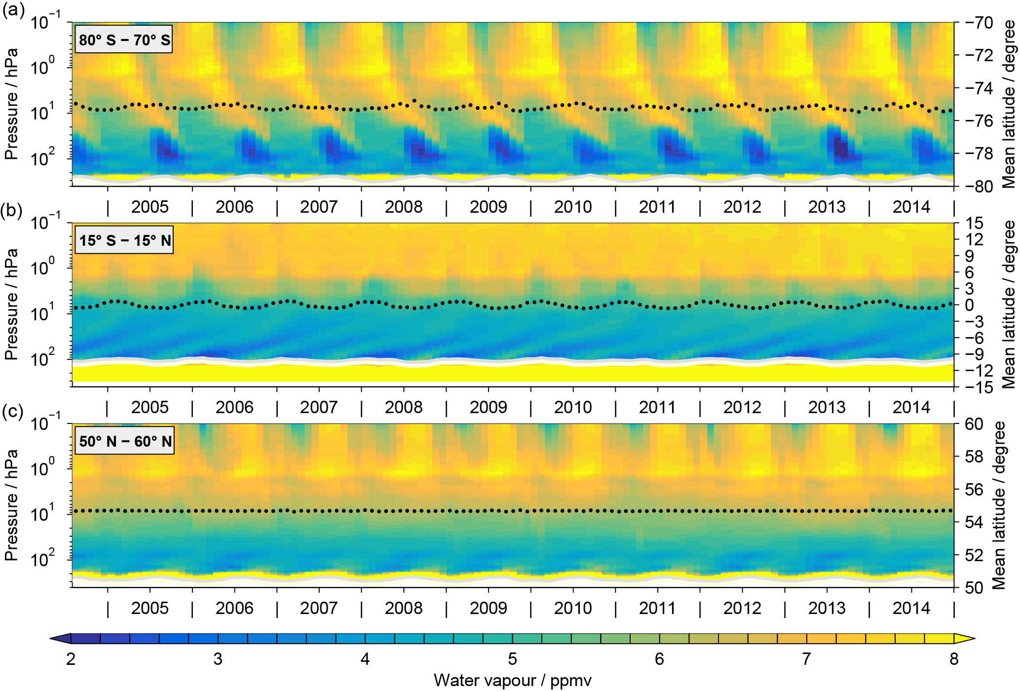
Figure 1Water vapour time series for the latitude bands 80∘ to 70∘ S (a), 15∘ S to 15∘ N (b) and 50∘ to 60∘ N (c) based on the MLS data. The light grey and white lines indicate the tropopause as derived from the MERRA reanalysis data. The black dots and the corresponding y axes on the right show the average latitude of the monthly mean data. White areas indicate that there are no data.
The comparison of the time series is then performed qualitatively for all data sets at the three latitude bands and at four selected altitudes covering the stratosphere and lower mesosphere (0.1, 3, 10 and 80 hPa). Subsequently, we assess the agreement of the data sets quantitatively in form of the spread over all data sets as well as the correlations and drifts among the individual data sets. While the example is based on absolute data, the comparison results presented in this section were derived from de-seasonalised data. The corresponding results based on absolute data (except for the drift) are provided in the Supplement.
4.1 General characteristics of the water vapour time series
Figure 1 shows contour time series of water vapour in the Antarctic (80∘–70∘ S), tropics (15∘ S–15∘ N) and mid-latitudes (50∘–60∘ N) based on the MLS data set for the time period 2004–2014. Here, the typical characteristics of the water vapour distributions in these latitude regions become visible. The water vapour distribution in the polar regions (Fig. 1 top) is determined by the following three processes: (1) dehydration of the lower stratosphere during polar winter caused by the sedimentation of ice containing polar stratospheric cloud particles (Fahey et al., 1990; Kelly et al., 1989); (2) vertical transport of dry/moist air. During polar winter, dry air from the upper mesosphere descends within the polar vortex to the upper stratosphere, while during summer and early autumn moist air from the upper stratosphere is transported into the mesosphere; (3) enhanced production of water vapour by methane oxidation during summer due to the higher insolation (Bates and Nicolet, 1950; Le Texier et al., 1988).
In the tropics (Fig. 1 middle), the most prominent feature in the water vapour time series is the “atmospheric tape recorder” (Mote et al., 1996). This feature is a consequence of the annual oscillation of dehydration (or freeze-drying) at the tropical tropopause due to the annual oscillation of the tropical tropopause temperature. The tape recorder signal is transported upwards to about 15 hPa by the ascending branch of the Brewer–Dobson circulation and maintains its integrity because of the subtropical mixing barrier in the lower stratosphere. Around the stratopause (∼1 hPa) a pronounced semi-annual oscillation is found that is induced by an interplay of transport and momentum deposition of different types of waves (Hamilton, 1998).
The water vapour distribution in the mid-latitudes (Fig. 1 bottom) is primarily influenced by transport within the Brewer–Dobson circulation and the overturning circulation in the mesosphere. In the lower stratosphere, low volume mixing ratios are transported from the lower latitudes to the mid-latitudes in late spring/early summer (Ploeger et al., 2013). Likewise, in the lower mesosphere the effect of upwelling in summer and downwelling in winter can be clearly seen, as described for the Antarctic.
4.2 Qualitative time series comparisons
In the following, the time series from the different satellite data sets are compared qualitatively. The time series in the three considered latitudes bands cover generally the time period from 1991 to 2014 (0.1 hPa), from 1986 to 2014 (3 and 10 hPa) and 1988 to 2014 (80 hPa). A necessary requirement for the analyses of the de-seasonalised time series was a minimum data set length of one year, ruling out some shorter data sets (see Sect. 4.1). However, these data sets are considered in the Supplement, where the time series in absolute terms derived from all satellite instruments considered in this study are provided (Figs. S3–S6). Some data sets, e.g. the MAESTRO data set, only have coverage up to the lowest pressure level (80 hPa) considered here and thus these data can only be found in bottom subfigures (Figs. 2–4 and S3–S6). Overall, 25 data sets have been considered in the comparison for the Antarctic while 24 data sets have been considered in the comparison for the tropics. In the Northern Hemisphere mid-latitudes, the best temporal and spatial coverage of the satellite data sets is found and therefore, 27 out of the 33 satellite data sets are considered in this comparison.
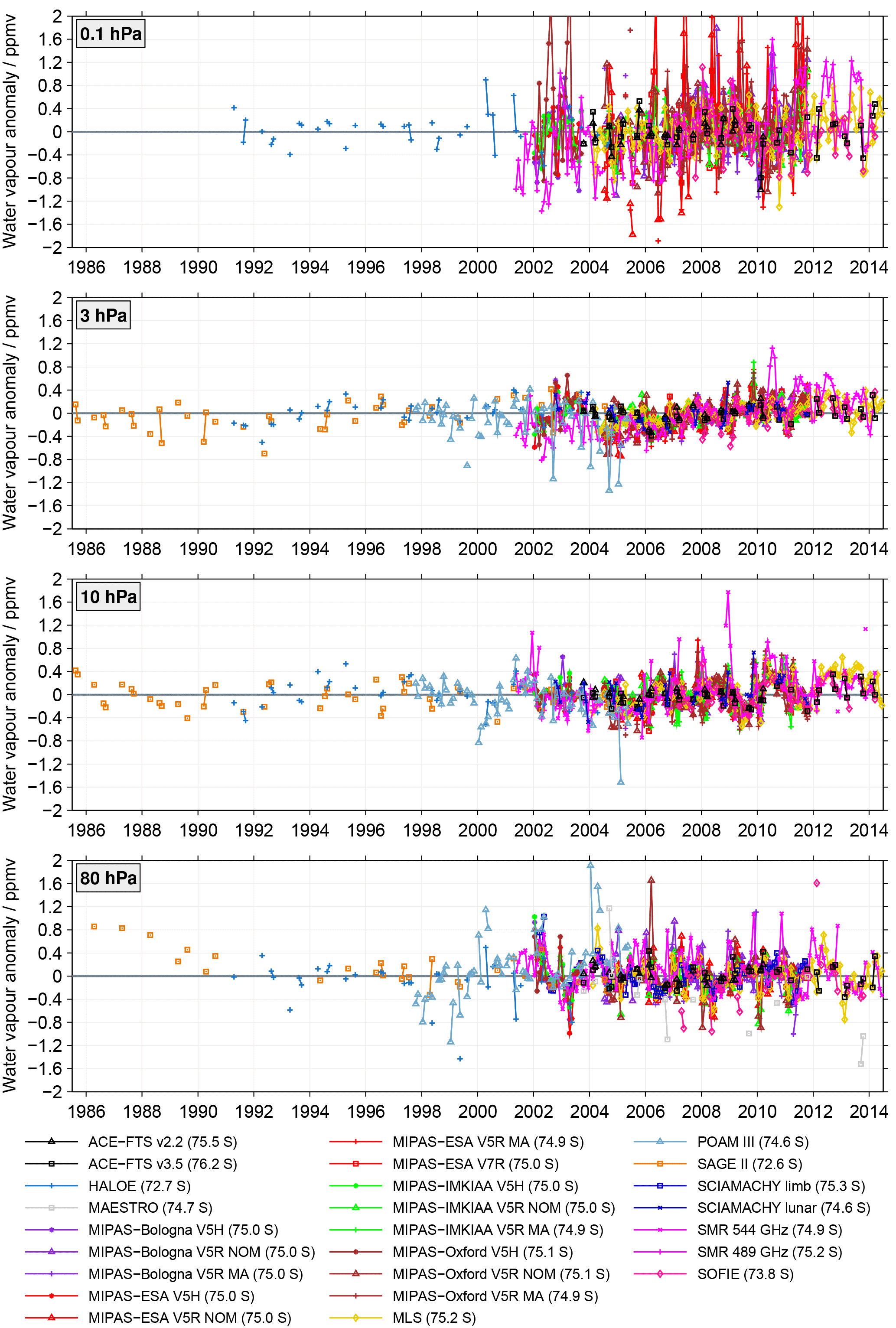
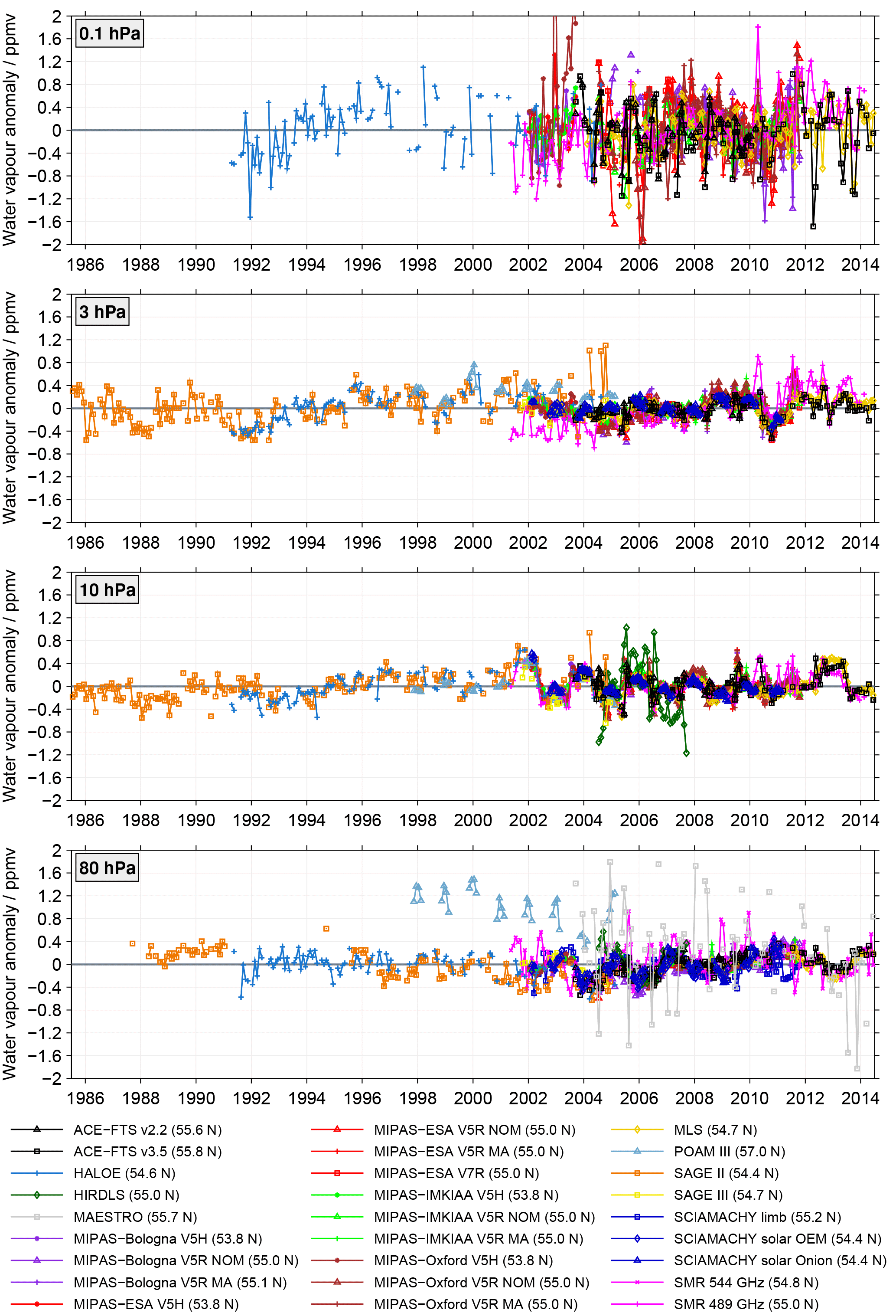
Figure 2De-seasonalised time series at four different altitudes considering the latitude band 80∘ to 70∘ S. In the legend the average latitude of the individual time series is indicated, which was calculated in two steps. First, for an individual monthly mean the latitudes of all profiles contributing to it were averaged. Any altitude dependence due to missing or screened data was ignored in this step. Finally, the mean latitudes over the entire time series were averaged. The same anomaly range (y axis) has been used in all panels so that the differences in the anomaly and the spread can be more easily compared. On the x axis the ticks are given in the middle of the year.
4.2.1 Antarctic (80∘–70∘ S)
Figure 2 shows the de-seasonalised water vapour time series for the southern polar latitudes. The HIRDLS, SCIAMACHY (solar occultation) and SAGE III observations have no coverage in this latitude region, while the GOMOS observations' coverage is too limited to allow derivation of de-seasonalised time series. In the de-seasonalised time series, a spread among the data sets can be found at the four altitudes considered in the comparison. The largest anomalies and the largest spread are found at 0.1 hPa (up to ±2 ppmv), while the smallest anomalies and thus the smallest spread is found at 3 hPa (generally in the range of ±0.4 ppmv).
At 0.1 hPa the time series start from 1991 onwards with HALOE, since SAGE II measurements are not available at this altitude. Large differences in the seasonal variation of the de-seasonalised time series are found, resulting in a considerable spread among the data sets, larger than at other altitudes. Large anomalies (up to ±2 ppmv), and thus large inter-annual variation, are found for the MIPAS-Oxford V5H, MIPAS-ESA V5R and MIPAS-ESA V7R data sets, while quite small anomalies are found for both ACE-FTS data sets. These large anomalies in the above mentioned MIPAS data sets are a consequence of the pronounced (spiky) seasonal variation in the absolute data (see Fig. S1 in the Supplement) that is difficult to be accounted for in the sinusoidal regression used for the de-seasonalisation.
Decadal changes in water vapour are found in the de-seasonalised time series at 3 hPa. Several periods of water vapour increases are followed by water vapour decreases. Negative anomalies are found around 1992 while positive anomalies are found around 1996 (HALOE). Water vapour then shows positive anomalies again in ∼2003 (HALOE, POAM III, SAGE II), followed by a decrease in 2003–2004, which again is followed by a slight increase in water vapour that lasts until 2010. From 2010 onwards water vapour remains unchanged. The last increase in water vapour is most strongly pronounced in SMR 489 GHz indicating a drift in the SMR 489 GHz data relative to the other data sets (see also Sect. 5.5). A large spread between the de-seasonalised time series is found between 1999 and 2004 (mainly between POAM III, SAGE II and SMR 489 GHz). Between 2005 and 2014, good agreement between the de-seasonalised time series is found. However, SMR 489 GHz has somewhat higher anomalies (from 2011 onwards) than the other satellite data sets.
At 10 hPa, the spread among the data sets is quite similar to that observed at 3 hPa, but the variability in water vapour is more pronounced. There is a decrease in the SAGE II de-seasonalised water vapour time series of 1986–1990. An increase in the de-seasonalised water vapour time series is found in POAM III around 2001. Also from 2009 onwards there seems to be a slight increase in water vapour in all data sets. The SMR 489 GHz de-seasonalised time series at 10 hPa is in good agreement with the de-seasonalised time series of the water vapour products derived from the other satellite instruments. However, the SMR 489 GHz as well as the SOFIE anomalies are low relative to MLS. This becomes quite obvious at the end of the time series (2012–2014), when only ACE-FTS, MLS, SMR 489 GHz and SOFIE were taking measurements. Also, the influence of the QBO is clearly visible at this altitude level. Distinct positive anomalies are found in 2007–2008, 2011 and 2013.
At 80 hPa the water vapour distribution is strongly influenced by dehydration (Sect. 5.1). The de-seasonalised time series at 80 hPa once again depict the spread between the individual instruments in this latitude band. At 80 hPa similar results as for 10 hPa are derived (except that here no long-term changes are visible). However, here the deviations between HALOE and SAGE II are smaller than at 10 and 3 hPa. As at 10 hPa, a decrease in the anomalies of the SAGE II de-seasonalised time series is found for 1986–1990. The de-seasonalised time series then remains constant until 1998 (HALOE and SAGE II). From 1998 onwards the spread between the data sets increases. There is an increase in the anomalies found in 2001, which is followed by a decrease, which lasts until 2004. Another decrease in water vapour is found in 2009. At 80 hPa, POAM III shows stronger inter-annual variation and higher/lower anomalies than at 10 and 3 hPa, depending on which year is considered.
4.2.2 Tropics (15∘ S–15∘ N)
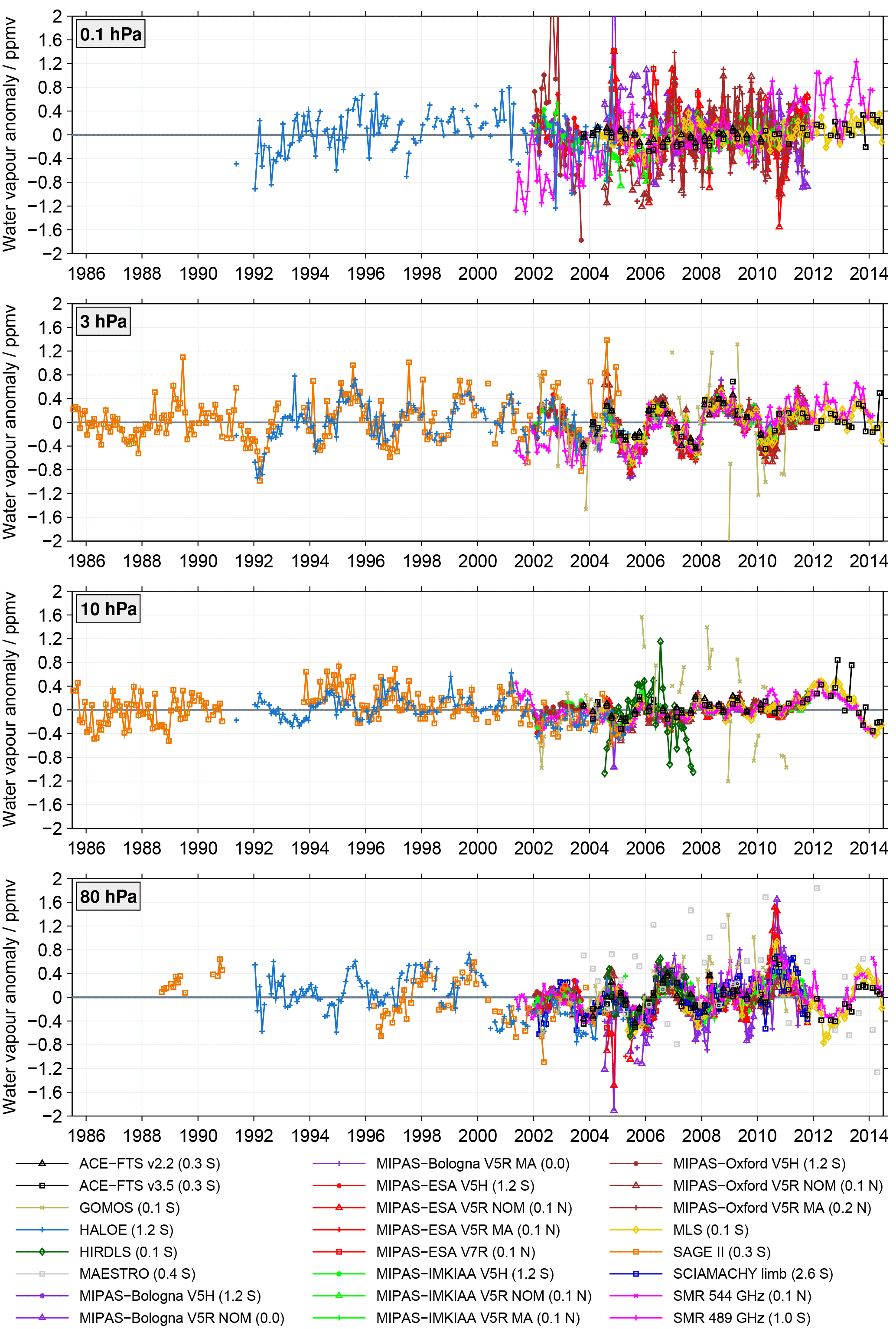
Figure 3 shows the de-seasonalised water vapour time series for the tropics. The POAM III, SAGE III, SCIAMACHY (solar and lunar occultation) and SOFIE data sets have no coverage in this latitude band. In the SAGE II time series some data gaps occur which are due to the aftermath of the Pinatubo eruption (resulting in unrealistically high water vapour values that were filtered out) as well as the “short events” between June 1993 and April 1994, when too few measurements were available (Taha et al., 2004). In the tropics, good consistency between the data sets is found except at 0.1 hPa, where again the spread between the data sets is largest. At 0.1 hPa some data sets exhibit larger anomalies (±1.2 ppmv; e.g. MIPAS-Oxford V5H and MIPAS-ESA V7R), while others exhibit rather small anomalies (±0.3 ppmv; e.g. ACE-FTS and MLS). The HIRDLS, GOMOS and MAESTRO (80 hPa) data sets show generally larger anomalies and thus larger spread than the other satellite data sets. The de-seasonalised time series in the tropics reflect the decadal changes in water vapour that have been documented in the literature, such as the drop in stratospheric water vapour after 2000 and in 2012 (Randel et al., 2004, 2006; Urban et al., 2014). Further, at 3 and 10 hPa, a variability in water vapour on an approximate 2-year timescale associated with the QBO is clearly visible.
At 0.1 hPa the time series starts in 1991 with the HALOE data set, which is also the only one available for these altitude and latitude regions until 2001. The de-seasonalised time series from HALOE shows an increase between 1992 and 1996 followed by a period with rather constant anomalies that lasts until 2001. Afterwards a decrease is visible until 2005. SMR 489 GHz observes, in contrast to HALOE, an increase in water vapour between 2001 and 2005. Therefore, at the beginning of the SMR 489 GHz record the anomalies at 0.1 hPa are clearly lower than those from HALOE or the other satellite data sets measuring from 2001 onwards. However, a large spread between the data sets is also found during this time period. A similar increase (but somewhat stronger) is found in the MIPAS Oxford V5H data set between 2001 and 2003, but here the anomalies are higher than the ones from the other satellite data sets. While the MIPAS Oxford V5H and SMR 489 GHz data sets show increasing anomalies, the other data sets show decreasing anomalies. From 2006 onwards all data sets show increasing anomalies. Between 2012 and 2014, ACE-FTS, MLS and SMR 489 GHz are the only data sets covering this time period and deviations among them are quite visible. SMR 489 GHz anomalies are higher and show larger inter-annual variability than ACE-FTS and MLS. MLS (together with ACE-FTS) exhibit generally the lowest anomalies (±0.3 ppmv) compared to the other satellite data sets at this altitude.
At 3 and 10 hPa the time series begins with SAGE II in 1986. From 1991 onwards HALOE observations are also available. Both SAGE II and HALOE provide here a much better representation of the temporal development of the water vapour time series and the inter-annual variability than in the Antarctic since both data sets have a much better temporal coverage in the tropics (see Figs. S1 and S2 in the Supplement). SAGE II shows somewhat larger anomalies than HALOE. Generally, the de-seasonalised time series show good agreement with each other at these two altitude levels (3 and 10 hPa). Further, at these altitude levels, the lowest anomalies and the lowest spread between the data sets is found, especially at 10 hPa. The deviations between MLS (or ACE-FTS) and SMR 489 GHz found during the time period 2012–2014 are still evident at 3 hPa but to a much lesser extent than at 0.1 hPa. At 3 hPa, inter-annual variations (with anomalies roughly on the order of ±1 ppmv) due to the QBO are clearly visible. At 10 hPa this variability is far less obvious. Also, the differences between SMR 489 GHz and the other data sets measuring during the time period 2001–2005 (SAGE II and HALOE) are found to a lesser extent at 3 hPa, but not at 10 hPa. The GOMOS data set exhibits large scatter. At 10 hPa the HIRDLS data set indicates stronger inter-annual variability than the other satellite instruments. This level is the uppermost altitude where HIRDLS can be retrieved and accordingly the data here are more uncertain. Both drops in water vapour, the one in 2001 and the one in 2012, are clearly visible in the de-seasonalised time series at 10 hPa. The latter one is strongly pronounced in the three remaining data sets covering that time period (ACE-FTS v3.5, MLS and SMR 489 GHz). There is also a clear variability on an approximate 2-year timescale associated with the QBO visible at this altitude level, although not at all times are as clearly pronounced as at 3 hPa.
Similar to the other three pressure levels, at 80 hPa relatively good agreement between SAGE II and HALOE is found. However, SAGE II typically shows somewhat lower anomalies than HALOE. At 80 hPa, higher variability with larger anomalies than at 10 and 3 hPa is found (generally around ±0.8 ppmv). The data sets agree well in terms of the inter-annual variation. The drops in 2000 and 2011 are consistently observed, as are the recoveries afterwards. This is also true for the pronounced QBO in 2006–2008. In 2005 the MIPAS-Bologna V5R NOM and MIPAS-ESA V5R NOM data sets show strong negative anomalies (up to −2 ppmv) which are not found in the other data sets. Similar behaviour of these data sets is found in 2011, when they show strong positive anomalies (up to 1.6 ppmv), while in the other satellite data sets, anomalies up to only 0.4–0.8 ppmv are found. MAESTRO shows strong scatter, mainly because 80 hPa is near the upper altitude limit of the MAESTRO water vapour retrieval. Another distinctive characteristic in the de-seasonalised time series at 80 hPa is the increase in water vapour that lasts until mid-2014 (ACE-FTS v3.5, MLS and SMR 544 GHz) which is anti-correlated with the time series at 10 hPa.
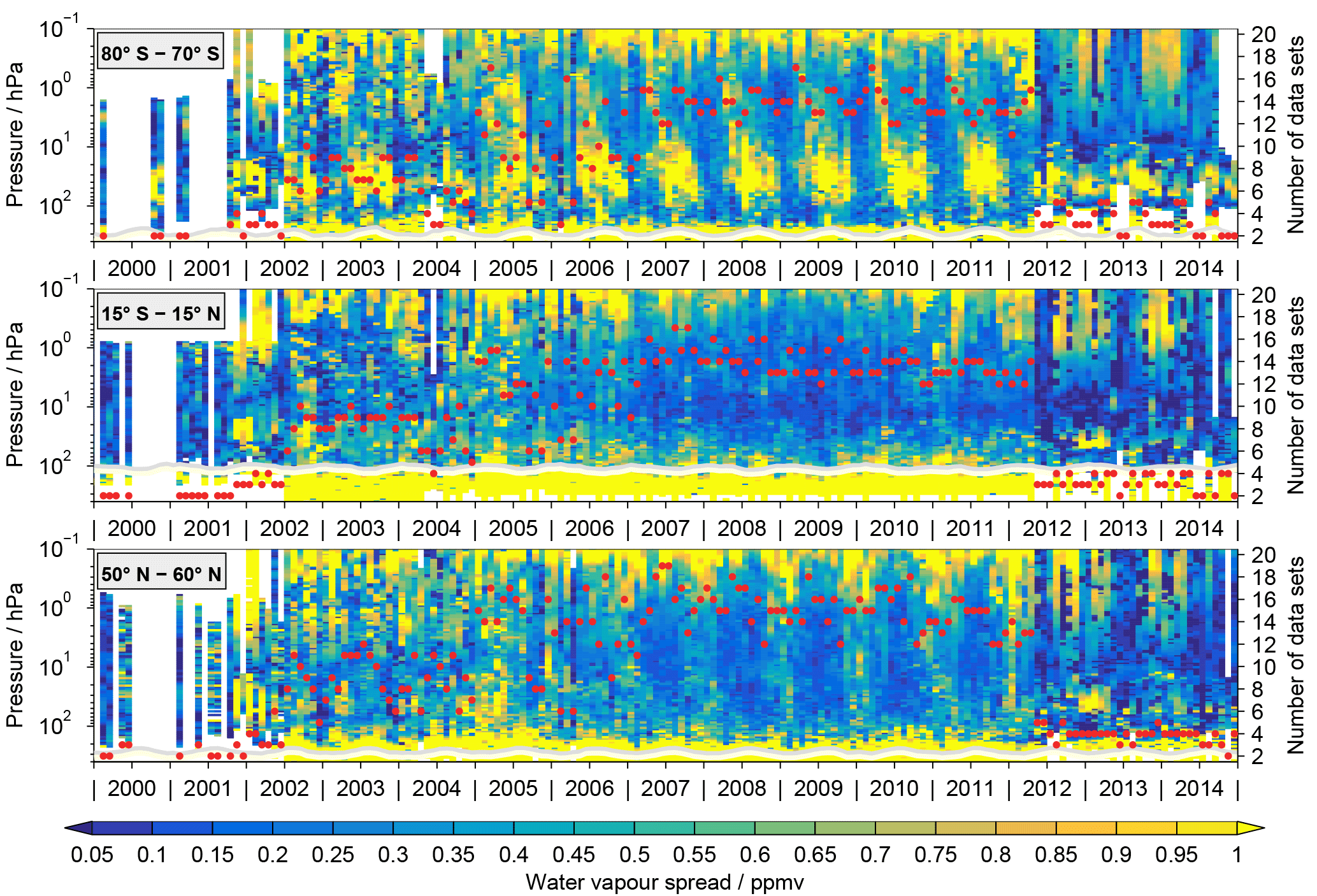
Figure 5The difference between the maximum and minimum volume mixing ratio among the different de-seasonalised data sets as a function of time and altitude for the three latitude bands. The light grey and white lines indicate the tropopause as derived from MERRA reanalysis data. The right y axes and the corresponding red dots indicate the maximum number of data sets available for this analysis at a given time considering all altitudes.
4.2.3 Northern mid-latitudes (50∘–60∘ N)
Figure 4 shows the de-seasonalised time series for the Northern Hemisphere mid-latitudes. The GOMOS, SCIAMACHY lunar and SOFIE data sets have no coverage in this latitude region. As for the other latitude bands the largest spread between the satellite data sets is found at 0.1 hPa. This is accompanied by large inter-annual variability. The ACE-FTS v3.5, MIPAS-Bologna V5H, MIPAS-Oxford V5H and SMR 489 GHz data sets are among the data sets showing the largest inter-annual variability and also the largest anomalies at 0.1 hPa. The MIPAS-Oxford V5H data set covers the time period of 2002–2004 and here the largest anomalies (exceeding 2 ppmv) are found. The largest negative anomalies are found in 2005 and 2006 with −1.6 and −2 ppmv, respectively. The differences between ACE-FTS v3.5 and the other satellite data sets become most pronounced at the end of the data record when only SMR 489 GHz and MLS were still measuring. Here, ACE-FTS v3.5 shows some larger variability. At this altitude, the drift in the SMR 489 GHz data set is again visible. The anomalies are typically more negative compared to the other data sets until 2004, while they are more positive after 2012. The HALOE data set indicates an increase in water vapour until about 1997 and a decrease afterwards. There appears to be a decrease in water vapour for all data sets from 2007 to 2010, followed by a pronounced increase that lasts until early 2012.
At 3 hPa, the de-seasonalised time series show generally good agreement, while at 10 hPa the best agreement is found. Differences at 3 hPa are that SMR 489 GHz exhibits lower anomalies during the time period 2001 to 2006 and higher anomalies than the other data sets from 2010 to 2014 and that SAGE II shows higher anomalies than the other satellite instruments at the end of their data record (2004–2005). Differences at 10 hPa are found in the time period 2004–2008, when SAGE II and HIRDLS show stronger inter-annual variability, and during 2010–2012, when SMR 489 GHz exhibits somewhat higher anomalies than the other satellite data sets. In both altitude levels, an increase in water vapour between 1992 and 2000 (10 hPa) and 1992 and 1998 (3 hPa) is found. The two water vapour drops that occurred after 2000 and in 2011 in the tropics (Randel et al., 2004, 2006; Urban et al., 2014) are also visible at 10 hPa in the Northern Hemisphere mid-latitudes, however with a temporal delay.
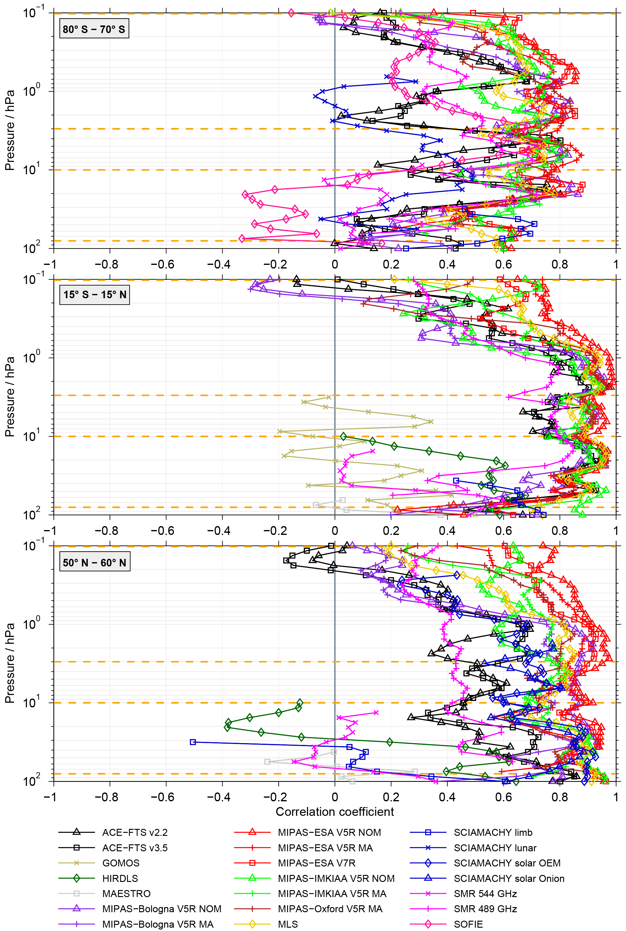
Figure 6Example correlations between de-seasonalised MIPAS-Oxford V5R NOM time series and those from other data sets. Results are only shown when the two data sets have an overlap of at least 12 valid monthly means. The dashed orange lines indicate the four altitudes for which the correlations between all data sets are shown in the following figures.
Although the inter-annual and decadal variability at 80 hPa is low, some satellite data sets (MAESTRO, POAM III and SMR 544 GHz) show larger deviations from the other satellite data sets. In the MAESTRO data, high inter-annual variability is found with anomalies reaching up to 1.6 ppmv. In this altitude region, MAESTRO has its best temporal coverage in the mid-latitudes, but still 80 hPa is at the upper limit of the MAESTRO measurements and therefore not every measured profile reaches that high up. This explains why higher variability (scatter) than in the other satellite data sets is found for the MAESTRO time series. POAM III exhibits much larger anomalies than the other satellite data sets (+1.2 ppmv compared to ±0.4 ppmv). Although the POAM III anomalies decrease with time, they still remain higher than the anomalies from the other satellite data sets. The differences between POAM III and the other satellite data sets are caused by the limited temporal sampling (only summer months are measured) of POAM III in this latitude region making the de-seasonalisation by regression apparently fail. In the SMR 544 GHz data set, larger inter-annual variability is found, but with much smaller anomalies than MAESTRO. In the SAGE II data, the anomalies are decreasing slightly in the time period 1987–2002. Further, there is some pronounced QBO alongside an overall increase from 2004 to 2012.
Overall, in the Northern Hemisphere mid-latitudes, the lowest inter-annual variability is found, especially at 80 hPa. Similar to the comparisons in the Antarctic and tropics, the largest inter-annual and decadal variability as well as the largest spread between the data sets is found at 0.1 hPa. The drops in stratospheric water vapour after 2000 and in 2011 that are observed in the tropics are also found at 10 hPa in the mid-latitudes, but with a temporal delay and to a lesser extent than in the tropics.
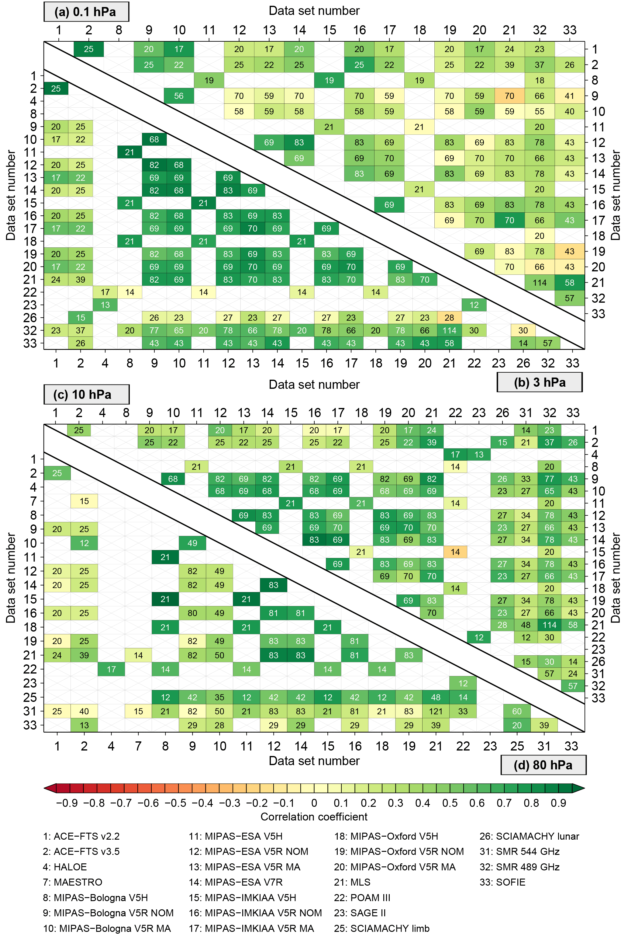
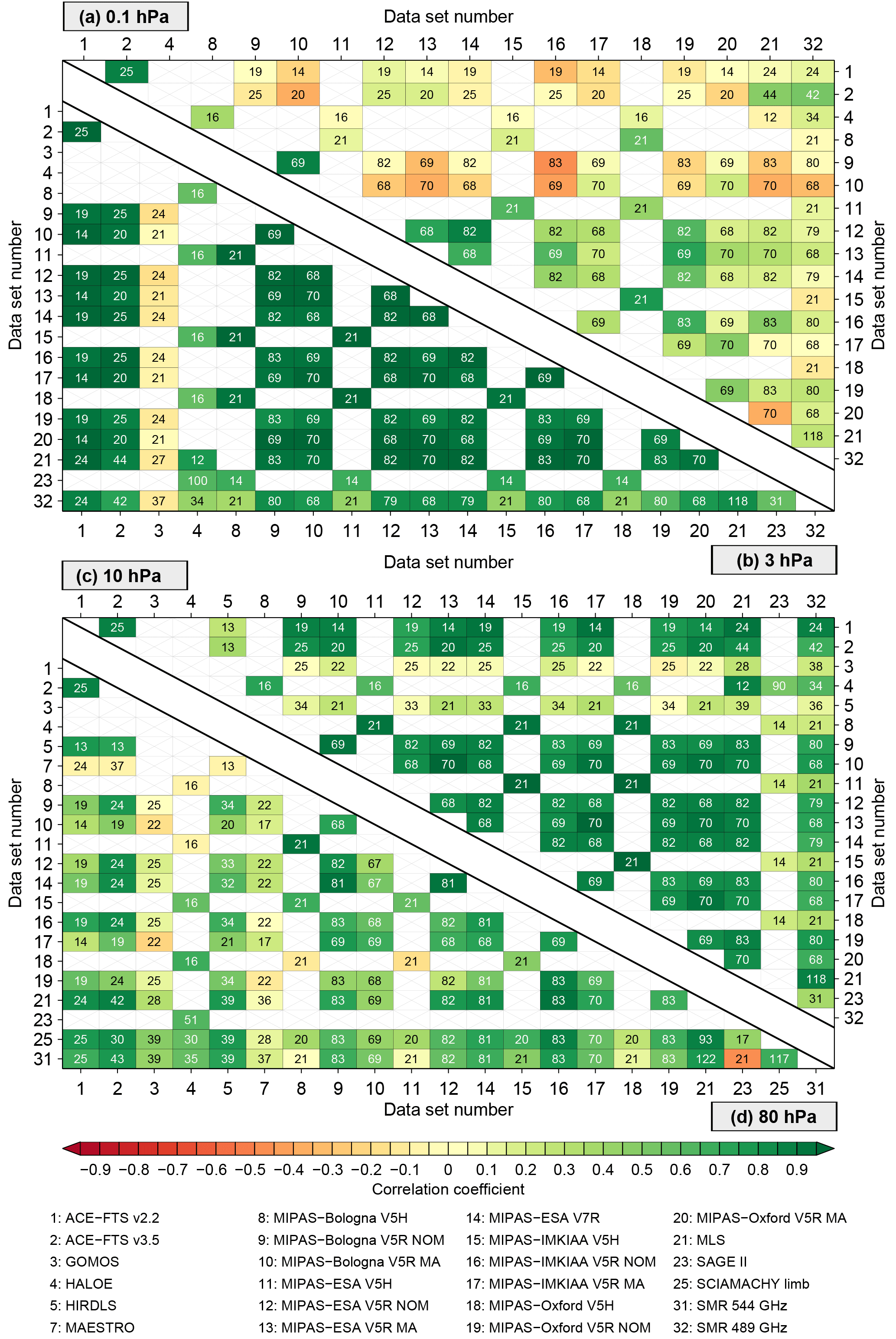
Figure 7The correlations between de-seasonalised time series in the latitude band between 80∘ and 70∘ S. The upper panel considers the 0.1 hPa (a) and 3 hPa (b) pressure levels, while in the lower panel the results at 10 hPa (c) and 80 hPa (d) are shown. Only data sets yielding any result at a given altitude are shown. Thus, the number of data sets can vary from altitude to altitude. Comparisons yielding no results are indicated by grey crosses. For comparisons with results (the coloured boxes) the number of months the two data sets actually overlap (i.e. both yield a valid monthly mean) are indicated.
4.3 Spread assessment
In the following, the spread between the data sets is quantitatively assessed to provide an estimate of the uncertainty in the observational database. Figure 5 shows the difference between the maximum and minimum volume mixing ratio among the different de-seasonalised water vapour data sets as a function of time and altitude for the three latitude bands: Antarctic, tropics and Northern Hemisphere mid-latitudes. The spread of the absolute time series is shown in the Supplement in Fig. S7. The spread is calculated for the years 2000–2014. Earlier years are not considered due to the lack of a sufficient number of satellite instruments measuring during that time period. Before 2000 only HALOE, POAM III and SAGE II data were available which results in a too sparse and not meaningful picture (similar to the gaps found for the early years in Fig. 5). The spread estimates become more meaningful as more satellite data sets become available. This can be seen from Fig. 5 for 2002 onwards. For the years 2000–2001 and 2012–2014 between two and four data sets were available. In these cases the differences among the data sets are not as pronounced and probably less meaningful than for the years 2002–2012, when the majority of satellite instruments were measuring.
In all three latitude bands the spread is large at the highest and lowest altitude level considered in this study, which correspond to the upper troposphere/tropopause region and the lower mesosphere. The large spread in these altitude regions is related to large uncertainties in the water vapour observations (e.g. due to increased measurement noise) as well as to the variability of the atmosphere and its different representation in the individual data sets. In addition, large spread is found in the Antarctic lower stratosphere (Fig. 5 top) in winter and spring, when the water vapour distribution in the lower stratosphere is affected by dehydration and transport of low water vapour from the mesosphere into the stratosphere (Sect. 5.1). In the tropics (Fig. 5 middle), the lowest spread compared to the other latitude bands is found. Increased values are found here as in the other regions at the highest and lowest levels. The spread is lowest in the time period 2006 to 2010. Similar behaviour is found for the mid-latitudes (Fig. 5 bottom), also here the spread seems to be lower around 10 hPa during the time period 2006–2010. The mid-latitudes show features similar to the tropics and polar regions. In the Northern Hemisphere mid-latitudes, the largest spread occurs in the lower stratosphere, where low water vapour is found due to air masses that are freeze dried when entering the stratosphere in the tropics (atmospheric tape recorder), and in the lower mesosphere due to the descent of air within the polar vortex.
4.4 Correlation assessment
To assess the temporal consistency between individual data sets, the correlation coefficients between all possible combinations of data sets are considered. In this section, the results for the de-seasonalised time series are presented, while the results for the absolute time series are given in the Supplement. We start by presenting an example correlation of the MIPAS-Oxford V5R NOM time series with those from the other data sets and then present all correlations in the form of matrices.
4.4.1 Correlation example
Figure 6 shows the correlation between the de-seasonalised MIPAS-Oxford V5R NOM time series and those from the other data sets for the Antarctic, tropics and the Northern Hemisphere mid-latitudes. The largest spread in the correlation between the satellite data sets is found in the Antarctic (Fig. 6 top), also where the lowest correlation over all altitude levels is found (rarely exceeding a correlation coefficient of 0.8). MIPAS-ESA V5R NOM and MIPAS-ESA V7R are among the data sets showing the highest correlation with MIPAS-Oxford V5R NOM over all altitude levels while the lowest correlation with MIPAS-Oxford V5R NOM is found for SCIAMACHY lunar throughout most altitudes. The SOFIE and SMR 544 GHz data sets show very low correlations (even negative for SOFIE) at the lowest altitude levels (below 10 hPa) as well as above 3 hPa (but here SMR 489 GHz instead of SMR 544 GHz). In between these altitudes levels the SOFIE and SMR 489 GHz data sets show similar correlation to MIPAS-Oxford V5R NOM as the other data sets.
In the tropics (Fig. 6 middle), the correlation coefficients vary between 0.8 and 1 for most data sets between 30 and 1 hPa. Low correlations are found for all data sets between 100 and 30 hPa, except the MIPAS-IMKIAA V5R NOM data set, which shows a high correlation (>0.8) up to 1 hPa with MIPAS-Oxford V5R NOM. The data sets that show the lowest correlation with MIPAS-Oxford V5R NOM (even in some occasions negative) are GOMOS and MAESTRO. These data sets thus deviate from the typical correlation of most other data sets. Above 60 hPa and above 25 hPa this is also true for HIRDLS and SMR 544 GHz, respectively. These two data sets show reasonable correlation with MIPAS-Oxford V5R NOM at the lowest altitude levels, but then the correlation coefficients decrease rapidly with increasing altitude, most likely due to increased measurement noise. At altitudes above 0.7 hPa the correlation decreases for all data sets and the spread between the data sets increases. For MIPAS-ESA V5R NOM, the correlation, although decreasing, remains rather high with a correlation coefficient of 0.7. The lowest correlation at 0.1 hPa is found for the ACE-FTS v2.2, ACE-FTS v3.5, MIPAS Bologna V5R NOM and MIPAS-Bologna V5R MA data sets.
In the Northern Hemisphere mid-latitudes (Fig. 6 bottom), the correlation coefficients vary between 0.4 and almost 1 in the altitude region between 0.7 hPa and 10 hPa depending on which data set is considered. The spread in the Northern Hemisphere mid-latitudes is almost as large as the spread in the Antarctic. Very high correlation (correlation coefficient of around 0.9–1) between MIPAS-Oxford V5R NOM and the other data sets is found at, for example, around 1 hPa for the MIPAS-ESA V5R NOM and MIPAS-ESA V7R data sets. The lowest correlation between MIPAS-Oxford V5R NOM and the other data sets is found above 1 hPa for the two ACE-FTS data sets while the SMR 489 GHz data set shows a rather low correlation throughout the entire altitude region considered in this study. Below 10 hPa the lowest correlations (even negative correlations) are found for HIRDLS, MAESTRO, SCIAMACHY limb and SMR 544 GHz data sets. These data sets also deviate from the usual spread in correlation of the data sets.
4.4.2 Correlation matrices
The correlation of all data sets is given in Figs. 7–9 in form of matrix plots for the three latitude bands and four altitude levels. In addition to the correlation coefficient, the number of months of overlap between the time series is given (requiring a minimum of 12 months; see Sect. 4.2.2). The same figures for the correlation of the absolute time series are given in the Supplement (Figs. S8–S10). The correlation matrix shown in Fig. 7 gives a good overview over the temporal consistency of all data sets in the Antarctic. The correlations between the data sets are generally positive (green), but in some cases negative correlations (red) are found, for example, in the case of the correlation between the MIPAS-IMKIAA V5H and POAM III data sets at 10 hPa or that between the MLS and SCIAMACHY lunar data sets at 3 hPa. However, in these two cases, the number of overlapping months is not that high (14 and 28) and this may explain the low correlation between these data sets. An example of where a negative correlation is found despite the high number of overlapping months (70) is the correlation between the MIPAS-Bologna V5R NOM and MLS data sets at 0.1 hPa. An example of a high number of overlapping months (114) and high correlation coefficient is the correlation between the MLS and SMR 489 GHz data sets at 10 hPa. Nevertheless, although in the Antarctic the correlation is generally positive, the correlation coefficient rarely exceeds 0.5. An exception is the 3 hPa level, where a generally high correlation among the MIPAS data sets is found. Similar behaviour between the MIPAS data sets is found at 10 hPa.
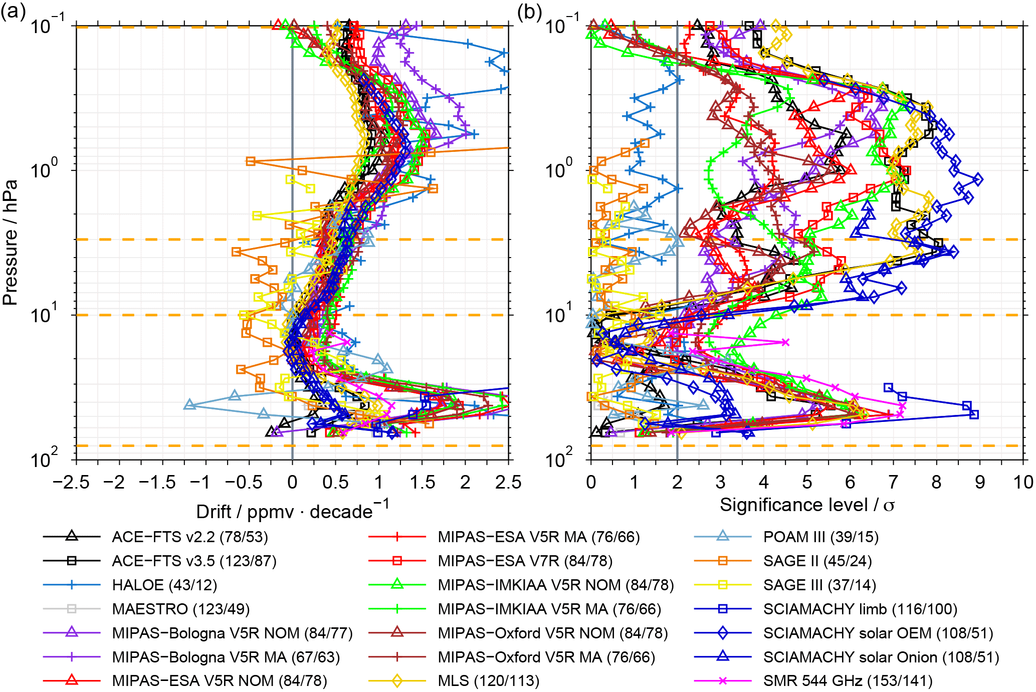
Figure 10The left panel shows the drifts between the de-seasonalised time series of the SMR 489 GHz data set and the other data sets. In the right panel the corresponding significance levels of the drift estimates are shown and the 2σ level is marked by a vertical line. This example considers the latitude band between 50∘ and 60∘ N. In the legend, the first number given in parentheses indicates the overlap period (over all altitudes) of the two data sets, i.e. the time between the first and the last month during which the data sets yield a valid monthly mean. Results are only shown here when this time period is at least 36 months. The second number indicates the number of months for which both data sets actually yield a valid monthly mean.
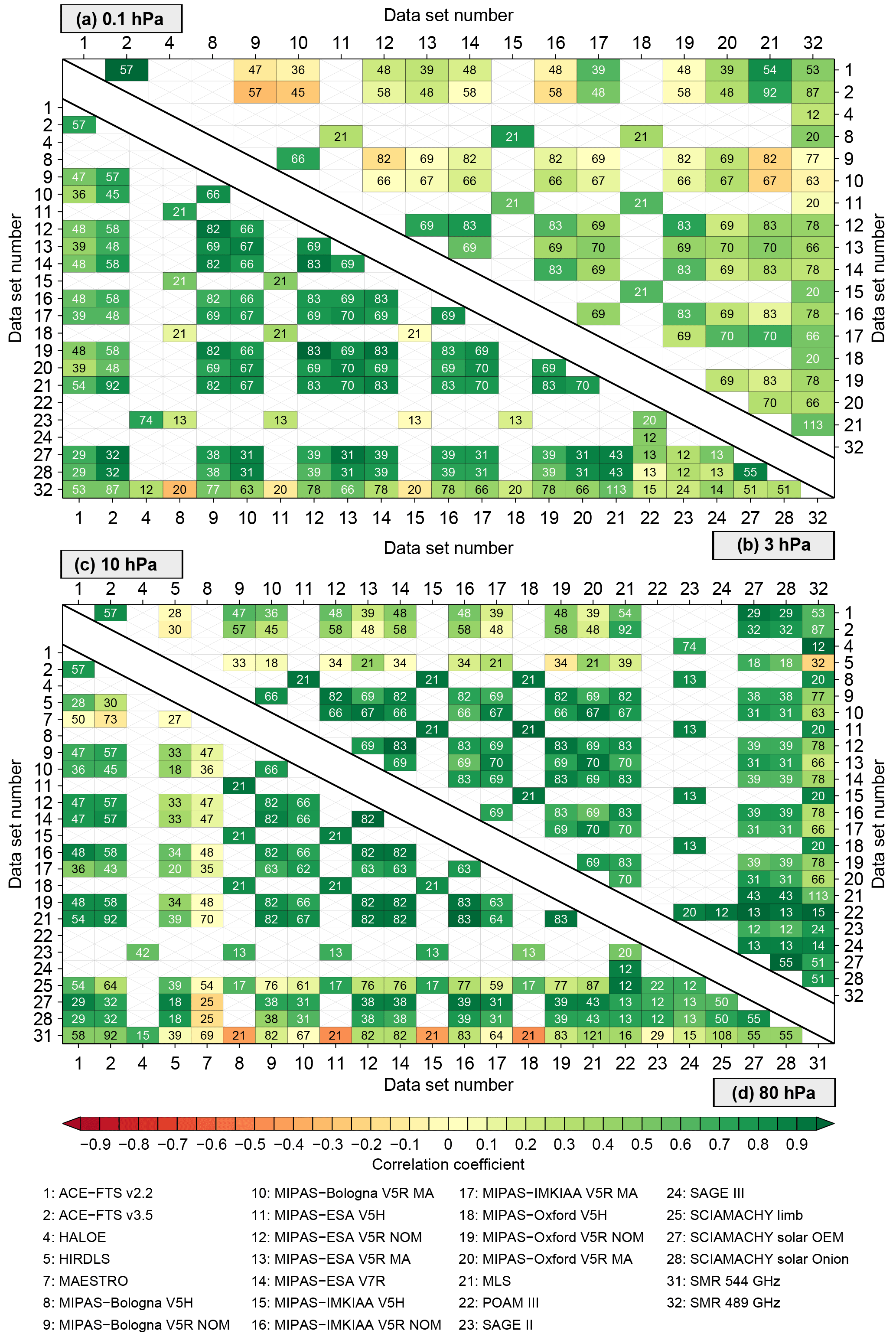
In Fig. 8 the correlation matrix for the tropics is shown. The large spread between the data sets we found in Fig. 6 at 0.1 hPa is also reflected in the correlations among all data sets. The same holds for the good correlations that are found at 3 and 10 hPa. An exception here is the GOMOS data set that shows negative correlations with all instruments at 3 hPa, but the number of overlapping months is rather low. At 80 hPa the spread between the data sets is not as large as at 0.1 hPa, but still larger than at 3 and 10 hPa. At 80 hPa occasionally negative correlations are found. This primarily concerns comparisons involving the GOMOS, HALOE, MAESTRO and MIPAS-Oxford V5H data sets. The lowest (negative) correlation is found between SMR 489 GHz and SAGE II data sets, but here the number of overlapping months (21) was also rather low.
The correlation matrix shown in Fig. 9 gives a good overview of the temporal consistency of all data sets in the mid-latitudes. The majority of the correlations are positive, but for some comparisons negative correlation is found. One such example is the correlation between the MIPAS Bologna V5H and SMR 489 GHz data sets at 3 hPa. However, again the number of overlapping months was rather low and may explain the negative correlation between these data sets. An example of negative correlation, despite a high number of overlapping months, is found between MIPAS-Bologna V5R NOM and MIPAS-Bologna-V5R-MA with MLS at 0.1 hPa. The correlation of these two data sets with the other data sets is also generally low at 0.1 hPa. Also, for the two ACE-FTS data sets the correlation of most data sets is often low despite a sufficient number of overlapping months. Positive correlations are found for the ACE-FTS v2.2/v3.5 data sets in comparison to the MIPAS-IMKIAA V5R MA, MIPAS-Oxford V5R MA, MLS and SMR 489 GHz. The highest correlation at 0.1 hPa is found between the two ACE-FTS data sets and between ACE-FTS v2.2 and MLS. At 3 and 10 hPa generally high correlations among the MIPAS data sets are found. At 10 hPa the correlation of HIRDLS with some data sets is high, but low with the other data sets. At 80 hPa low correlations between MAESTRO and all other instruments are found.
In summary, a high number of overlapping months does not necessarily guarantee a good correlation between two data sets, but generally the chances are quite high if this is the case. On the other hand, if data sets overlap only for a low number of months, good agreement between these data sets can still be found. Therefore, for assessing the agreement between two data sets, both the number of overlapping months and the correlation coefficient should be taken into account. The correlation assessment again confirms what we found before from the qualitative time series comparison, namely that the best agreement between the satellite data sets is found in the tropics, while in the Antarctic and Northern Hemisphere mid-latitudes a large spread between the data sets is found. Generally, the lowest correlations are found in the Antarctic. Further, in each latitude band the correlation is lower in the lower stratosphere and lower mesosphere than in the middle stratosphere.
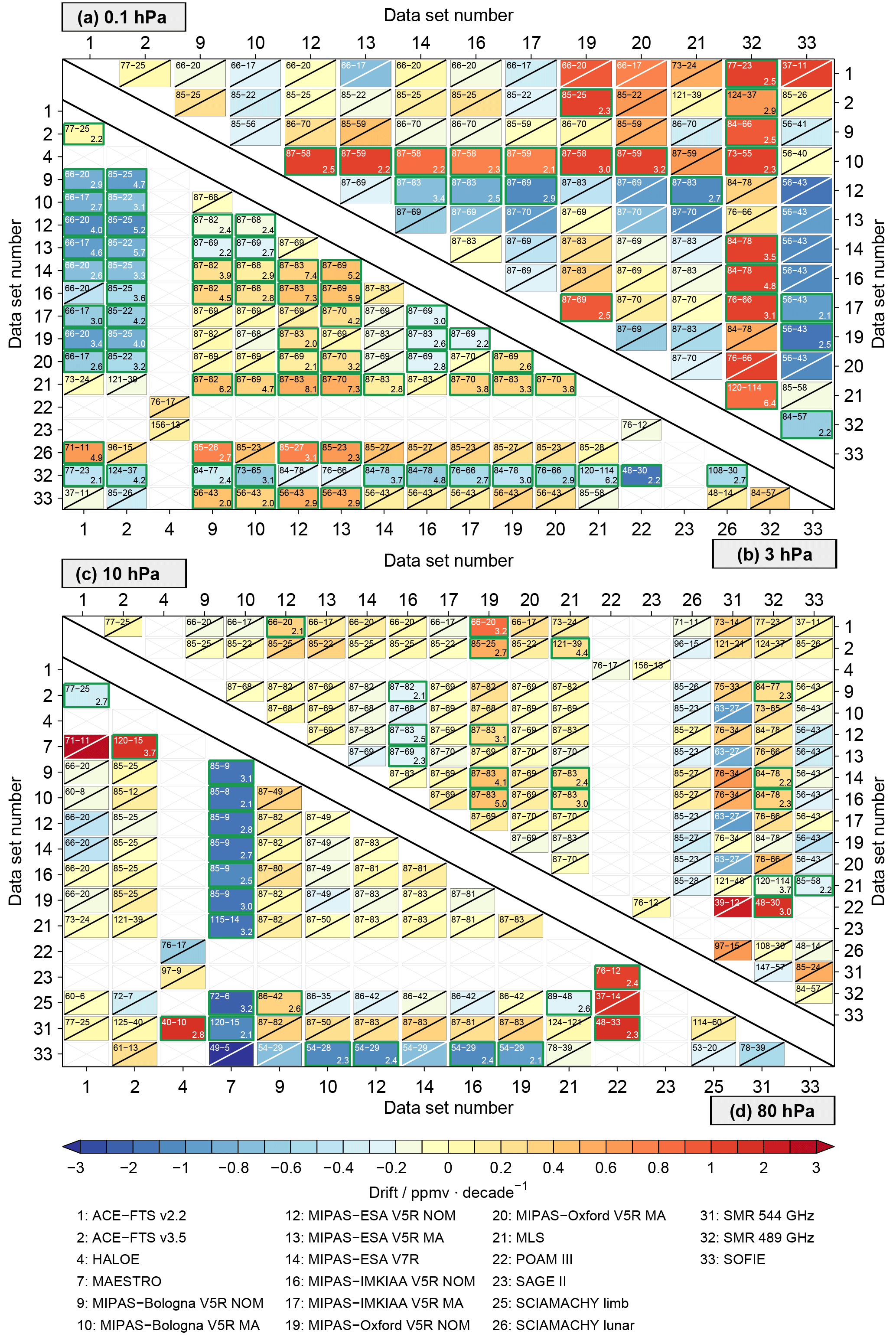
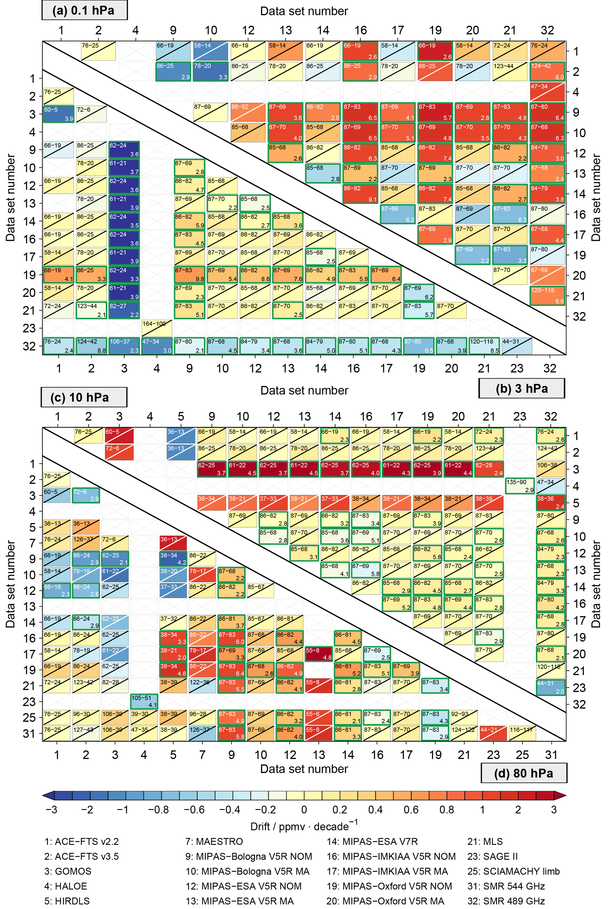
Figure 11Drifts between the different data sets in the latitude band between 80∘ and 70∘ S at four specific altitudes. The drift estimates are based on the difference time series between the data sets given on the x axis and the data sets given on the y axis. Additional information is given in the result boxes: the overall time period the two data sets overlap, how many months the data sets actually overlap (upper left corner) and if the drifts are significant (green frame) or not significant (slant) at the 2σ uncertainty level. The significance level is given in the lower right corner in cases where the drift is significant.
4.5 Drift assessment
In addition to the spread and correlations, the drifts among the satellite data sets are considered. As drift we consider the linear change of the difference between two time series, which indicates if the longer-term variation of the two time series is the same or not (Sect. 4.3). As before, we start with an example. In Fig. 10 the drifts between the de-seasonalised time series of the SMR 489 GHz and all other data sets are shown for the Northern Hemisphere mid-latitudes (left panel) as well as the corresponding significance level (right panel). The significance level is given by the absolute ratio of the drift to the drift uncertainty. We consider a drift as statistically significant when the significance level is larger than 2σ (corresponding to the 95 % confidence level).
4.5.1 Drift example
Figure 10 shows that below 20 hPa large drifts (up to 2.5 ppmv decade−1 and even higher) are found between SMR 489 GHz and the other satellite data sets. In the altitude region between 20 and 1 hPa, good consistency between the satellite data sets is found despite the different time periods of measurements. The smallest drifts, ranging from about 0 to 0.5 ppmv decade−1, are found around 20 hPa. The drifts consistently increase with altitude and maximise around 0.4 hPa. Above 1 hPa the drifts of SMR 489 GHz vary between about 0.75 and 1.5 ppmv decade−1 depending on which data set the SMR 489 GHz data set is compared to, but decrease with altitude towards 0.1 hPa. The drifts range here between 0 and 1.25 ppmv decade−1. The drifts between SMR 489 GHz and the other satellite data sets are in most cases significant at the 2σ uncertainty level as can be seen from Fig. 10 (right panel). Larger drifts between SMR 489 GHz and the other data sets that obviously deviate from the majority of data sets are found for the comparison to the POAM III, SAGE II, SAGE III and HALOE data sets. However, this is due to the fact that for these data sets not only the overlap period with SMR 489 GHz is relatively short (4 years, 2001–2005), but also the number of months for which both data sets actually yield a valid monthly mean is small (see numbers given in figure legend). Additionally, these drifts are in most cases not statistically significant at the 2σ uncertainty level.
4.5.2 Drift matrices
In Figs. 11–13 the drift estimates between the time series of all data sets are summarised as matrix plots for the three latitude bands and four altitudes. In the matrix plots, data sets are only shown if they yield any result at a given altitude. The drift estimates are based on the difference time series between the data sets given on the x axis and the data sets given on the y axis. Additional information that is given in the matrix plots includes the overlap period of the two data sets, how many months the two data sets actually overlap and if the drift is significant or not at the 2σ uncertainty level as well as the corresponding significance level for significant drift.
In the Antarctic (Fig. 11), almost no significant drifts are found between the satellite data sets at the two lowest altitude levels (80 and 10 hPa). An exception here is the MAESTRO data set which shows a significant (negative) drift of −2 to −3 ppmv decade−1 (significance level up to 3.7) and POAM III which shows a significant positive drift (2 to 3 ppmv decade−1) compared to SAGE II and SMR 544 GHz (at 80 hPa). While the overall time period MAESTRO had overlap with other data sets was sufficiently long (>85 months), the number of coincident months for these data sets was rather low (9 months). Further, at 80 hPa, a significant negative drift is found between some MIPAS data sets and SOFIE. At 10 hPa, a significant (positive) drift (0.8 ppmv decade−1) is found between the MIPAS-Oxford V5R NOM and ACE-FTS v2.2 data sets (significance level of 3.2) and of 2 ppmv decade−1 between the SMR 489 GHz and POAM III data sets (significance level 3.0). Additionally, significant drifts are found between different MIPAS data sets relative to SMR 489 GHz and between the MLS and SMR data sets. At 3 hPa most drifts are significant. Most MIPAS data sets exhibit significant positive drifts relative to the ACE-FTS (significance level up to 5.7) and MLS (significance level up to 8.1) data sets. While in the comparisons to the ACE-FTS data sets the actual number of overlapping months is limited, this is not the case in the comparison to MLS. As before, for the SMR 489 GHz data set significant positive drifts are found (significance level up to 4.8) relative to most other data sets. A large variety of drifts is found at 0.1 hPa, but in most cases the drift is not significant. Data sets for which most drifts are significant at this altitude level are SMR 489 GHz (>2 ppmv decade−1, significance level up to 6.4) and MIPAS-Bologna V5R MA (significance level up to 3.2).
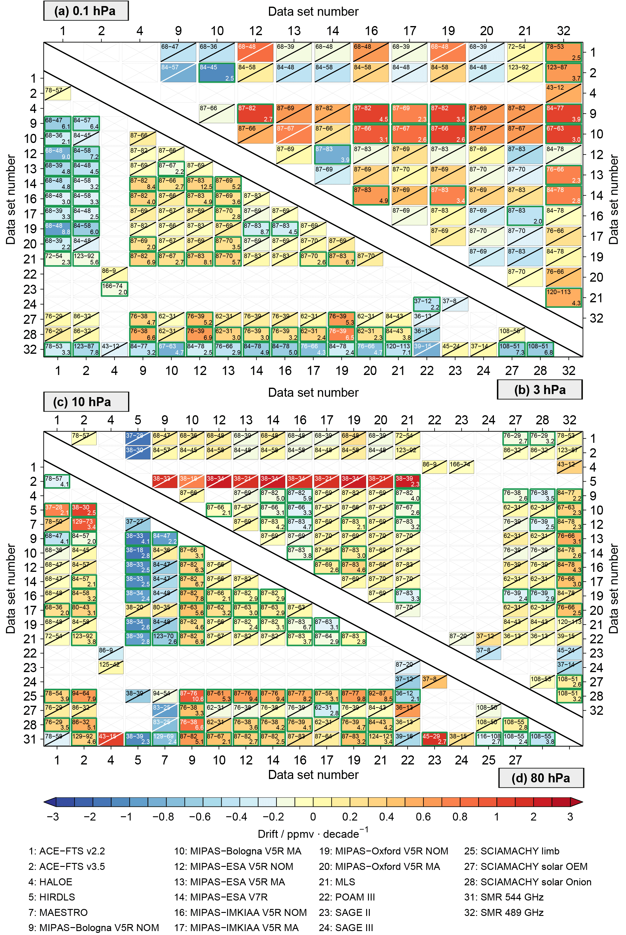
In the tropics (Fig. 12), larger drifts are found than in the Antarctic, especially at 0.1 hPa. Here, most drifts are significant. Significant drifts are found for the MIPAS-Bologna V5R NOM, MIPAS-Bologna V5R MA, MIPAS-ESA V5R, MIPAS-IMKIAA V5R NOM, MIPAS-Oxford V5R NOM and SMR 489 GHz data sets. For example, for MIPAS-Bologna V5R NOM and MIPAS-Bologna V5R MA drift (significance level up to 6.5) in comparison to most other satellite data sets is found. For MIPAS-Bologna V5R NOM this is also the case at 3 hPa (significance level up to 9.8). Large negative drifts are found for GOMOS ( ppmv decade−1, significance level up to 3.9) compared to most data sets. Also for SMR 489 GHz significant positive drifts (up to ∼1 ppmv decade−1, significance level up to 8.5) for almost all data sets are found at 3 hPa. Good consistency is found among the MIPAS data sets. The drifts are low and in most cases not significant. An exception here is MIPAS-Oxford V5R NOM (∼0.6–1 ppmv decade−1, significance level up to 9.8). For the tropics the best agreement among the data sets is found at 10 hPa. In most cases the drift is not significant and in cases where the drift is significant the drifts are relatively low with 0.2–0.4 ppmv decade−1. Larger drifts are found at this altitude for GOMOS (up to −3 ppmv decade−1) and HIRDLS (up to −2 ppmv decade−1). For GOMOS the drifts are significant in most cases (significance level up to 4.3), while this is not the case for HIRDLS.
At 80 hPa a wide variety is found. Some data sets show positive drift, some negative. In some cases the drift is significant and in other cases not. For example, a positive drift (2 ppmv decade−1) relative to almost all data sets is found for MIPAS-Bologna V5R NOM (significance level up to 6.4). For the HIRDLS data set a significant positive drift (also ∼2 ppmv decade−1) is found compared to MIPAS-IMKIAA V5R NOM, MIPAS-IMKIAA-V5R MA and MIPAS-Oxford V5R NOM (significance level 2.0–4.6). A large drift (>3 ppmv decade−1) at this altitude level is found for MIPAS-ESA V5R MA compared to MIPAS-IMKIAA V5R NOM (significance level 4.8). Also the MIPAS-Oxford V5R NOM shows significant drifts compared to a number of data sets.
The patterns of the estimated drifts in the Northern Hemisphere mid-latitudes shown in Fig. 13 are quite similar to the drifts in the tropics and Antarctica. However, the estimated change in ppmv decade−1 seems to be somewhat lower in the mid-latitudes than in the tropics or Antarctic. The highest variety is again found at 0.1 hPa. Similar to the tropics significant drifts are found, e.g., for the MIPAS-Bologna V5R NOM and MIPAS-Bologna V5R MA (up to −2 ppmv decade−1, significance level up to 3.9) data sets relative to the SMR 489 GHz data set. At 3 hPa, for most data sets the drifts are small and/or not significant. Significant negative drifts are found for both ACE-FTS data sets and for SMR 489 GHz. For SMR 489 GHz drift is found relative to most other data sets which is also in most cases significant. At 10 hPa HIRDLS shows pronounced drifts compared to the other data sets. However, these drifts are not significant except for the comparison with MLS (drift of 3 ppmv decade−1, significance level 2.3). Otherwise for most data sets the drifts are small and/or not significant at 10 and 80 hPa. Exceptions are HIRDLS (−2 ppmv decade−1) and MAESTRO (−1 ppmv decade−1), which show negative drift at 80 hPa. For HIRDLS in most cases the drift is significant (significance level up to 4.1), but for MAESTRO in most cases not. For MIPAS-Bologna-V5R NOM significant positive drifts are found for all instruments that are in most cases around 0.2–0.4 ppmv decade−1, but higher compared to HIRDLS (significance level 4.1), MAESTRO (significance level 2.2), SCIAMACHY limb (significance level 10.6) and SCIAMACHY solar OEM (significance level 6.6). Other data sets for which drifts are found compared to most other data sets are SCIAMACHY limb, SCIAMACHY solar Onion and SMR 489 GHz.
In the framework of the second SPARC water vapour assessment, time series of stratospheric and lower mesospheric water vapour derived from satellite observations were compared. The comparison results presented comprise 33 data sets from 15 satellite instruments. These comparisons provide a comprehensive overview of the typical uncertainties in the observational database that should be considered in the future in observational and modelling studies addressing stratospheric and lower mesospheric water vapour variability and trends.
The time series comparison was performed for three latitude bands: the Antarctic (80–70∘ S), the tropics (15∘ S–15∘ N) and the Northern Hemisphere mid-latitudes (50∘–60∘ N) at four altitudes levels (0.1, 3, 10, 80 hPa) covering the stratosphere and lower mesosphere. The combined temporal coverage of observations from the 15 satellite instruments allows consideration of the time period 1986–2014. In addition to the qualitative comparison of the time series, a quantitative comparison was provided based on the spread, correlation and drift between the individual time series.
The qualitative time series comparison shows that the largest differences between the de-seasonalised time series are in the Antarctic and in the lower mesosphere (0.1 hPa) and tropopause region (80 hPa). In the stratosphere (3 and 10 hPa) and the tropics, good agreement between the satellite data sets was found. These differences were quantitatively confirmed by the correlation assessment, where the best agreement between the satellite data sets was also found in the tropics, while in Antarctic and Northern Hemisphere mid-latitudes, large spread between the data sets was found. Generally, the lowest correlations between the individual data sets were found in the Antarctic. In each latitude band the correlation was lower in the lower stratosphere and lower mesosphere than in the middle stratosphere.
There are multiple factors that give rise to the observed differences between the individual data sets. A thorough discussion on this is given in Lossow et al. (2017b). From this study we know that the most important contributions arise from differences in temporal and spatial sampling, the influence of clouds or NLTE effects. Other factors include systematic differences, for example calibration problems. However, for the time series comparison we would rank sampling biases and systematic errors as the most important reasons for the differences as was discussed by Toohey et al. (2013) based on trace gas climatologies.
The reason why the largest differences between the data sets are found in the tropopause region, in the lower mesosphere and in the Antarctic is that these are also the locations where the highest variability in water vapour is found. Given the limited vertical resolution of the satellite data sets, tropospheric influences start to play a role near the tropopause. Sampling differences become more pronounced due to the large variability, e.g. due to the fact that the satellite observations are influenced differently by clouds. In the lower mesosphere, diurnal variation becomes more important. The satellite data sets do not have the same local time coverage. For example there is the influence of NLTE effects in most MIPAS data sets except MIPAS-IMKIAA V5R MA, where these NLTE effect are explicitly considered. Larger deviations in the lower mesosphere occur, e.g. in the case of the MIPAS NOM data sets, which are close to their upper retrieval limit there, and thus more uncertain.
Less agreement between the data sets was found for the Antarctic, especially in the lower stratosphere in winter and spring when dehydration occurs. Large differences between the data sets were found in both the absolute and de-seasonalised data. In the absolute data, these differences are primarily caused by differences in the influence of clouds on the measurements. However, sampling biases can also play a role. In the de-seasonalised data some differences between the data sets could be related to the de-seasonalisation approach used in our study (e.g. POAM III). Since the dehydration is more a seasonal phenomenon, and accordingly is less characterised by a sinusoidal behaviour, the usage of sinusoidal functions for the de-seasonalisation is not optimal. Instead, the average approach (see Sect. 4.1) would be more suitable for de-seasonalisation in this region.
In addition to the assessment of the spread and correlations, the drifts between the individual data sets were also assessed, which indicates if the longer-term variations (drifts) of two time series are the same or not. From the drift comparison we found that the drift patterns are quite similar for the three latitude bands considered. The drifts are highest at the highest and lowest considered altitude levels (0.1 and 80 hPa). The majority of significant drifts were found in the tropics (the latitude region with the lowest spread/variability), which makes the drift detection considerably easier. Further, it is possible that some of the drifts (especially for the low-density samplers) are caused by sampling biases (Damadeo et al., 2018). The same drift approach as used here has been used by Lossow et al. (2018) to calculate drifts from profile-to-profile comparisons (using coincident data). However, no statistically significant difference was found between the two sets of drifts in 95 % of the comparisons.
Further, from the drift assessment we found that the MIPAS data sets show positive drifts relative to the ACE-FTS data sets in the Antarctic and Northern Hemisphere mid-latitudes at 3 hPa. Interestingly, no drifts of MIPAS relative to ACE-FTS are found in the tropics. The reason for this is currently not understood. The drifts found in the MIPAS data sets are consistent with the time dependence unaccounted for in the correction coefficient for the non-linearity in the detector response function used in the data sets based on calibration version 5 (Walker and Stiller, 2018). Some improvement is seen in the MIPAS ESA V7R NOM data set, where a time dependence of the correction coefficient is implemented, though not at all altitudes. Additionally, even drifts among the different MIPAS data sets were found. This might be related to the different retrieval choices (as well as to the usage of different micro-windows) by the different processors and to sampling differences between the NOM and MA observations. Further, from the drift comparison, we found that the SMR 489 GHz data set shows a significant drift relative to the other data sets, except at around 10 hPa. The drifts of the SMR 489 GHz data set are largest at around 50 and 0.5 hPa with approximately 1.5 and >2 ppmv decade−1, respectively depending on the data set used for comparison.
Further, within this assessment study we encountered the following difficulties in our analyses using the HIRDLS, GOMOS and MAESTRO data sets. The GOMOS time series exhibit larger scatter from month to month (coverage only in the tropics for de-seasonalised data here) despite extended screening (Walker and Stiller, 2018), resulting in low correlations to the other data sets and pronounced negative drifts at 10 and 3 hPa. The quality of the HIRDLS data set deteriorates towards 10 hPa, resulting in low correlations, larger anomalies and larger drifts. However, the drifts were mostly not statistically significant. It should be noted here that in addition to correcting for the effects of the obstruction in the optics, changes in the calibration were made within the HIRDLS mission (Gille et al., 2008, 2012). This change in calibration may also have an influence on the drift estimates. The MAESTRO data set encounters large uncertainty (noise) at 80 hPa (in the correlations and drifts) which is related to the vicinity to the uppermost limit of these retrievals. Similar behaviour is also found for the SCIAMACHY limb and the SMR 544 GHz data sets.
Nevertheless, although the water vapour data sets have been thoroughly assessed in this study it is difficult or rather impossible to decide which data set is most suitable for future modelling and observational studies. This can only be answered with respect to the specific scientific application to which the data set is intended to be applied. For future studies, e.g. on water vapour trends, we can state that the data sets that provide the longest measurement record with high spatial and temporal coverage have an advantage over the ones which provide only observations in specific latitude bands and/or altitude regions. For data sets that show drift relative to other data sets (e.g. SMR 489 GHz), a drift has to be taken into account, and data sets that are simply too short (less than 1 year; e.g. ILAS-II and SMILES) cannot be used for trend studies at all. Thus, from our assessment we find that most data sets can be considered in future observational and modelling studies, e.g addressing stratospheric and lower mesospheric water vapour variability and trends, if data set specific characteristics (e.g. an instrument drift) and restrictions (e.g. spatial and temporal coverage) are taken into account.
Data are available upon request.
The supplement related to this article is available online at: https://doi.org/10.5194/amt-11-4435-2018-supplement.
The study was designed by JU, FK and SL with contributions from the WAVAS-II core members GS, KR, JCG, MK, GEN, WGR and KAW. FK wrote the manuscript and SL performed the analyses and contributed to the writing of the manuscript. JU performed the first version of the analyses. GS helped with the selection of results to be presented in the paper. KHR contributed to the discussion of the results. Satellite data used in this study were provided by GPS, JPB, RD, PE, MGC, JG, YK, MK, SN, PR, WGR, AR, CS, KAW and KW. Valuable comments on the manuscript were provided by GPS, KHR, RPD, PR, MG, SN, CS, JG, AR and KW.
The authors declare that they have no competing interests.
This article is part of the special issue “Water vapour in the upper troposphere and middle atmosphere: a WCRP/SPARC satellite data quality assessment including biases, variability, and drifts (ACP/AMT/ESSD inter-journal SI)”. It does not belong to a conference.
The Atmospheric Chemistry Experiment (ACE), also known as SCISAT, is a
Canadian-led mission mainly supported by the Canadian Space Agency and the
Natural Sciences and Engineering Research Council of Canada. We would like to
thank the European Space Agency (ESA) for making the MIPAS level-1b data set
available. MLS data were obtained from the NASA Goddard Earth Sciences and
Information Center. Work at the Jet Propulsion Laboratory, California
Institute of Technology, was done under contract with the National
Aeronautics and Space Administration. SCIAMACHY spectral data have been
provided by ESA. The work on the SCIAMACHY water vapour data products has
been funded by DLR (German Aerospace Center) and the University of Bremen.
The SCIAMACHY limb water vapour data set v3.01 is a result of the DFG (German
Research Council) Research Unit “Stratospheric Change and its Role for
Climate Prediction” (SHARP) and the ESA SPIN (ESA SPARC Initiative) project
and were partly calculated using resources of the German HLRN
(High-Performance Computer Center North). We would like to thank Mark Hervig
for providing the SOFIE data and Takafumi Sugita for providing the ILAS-II
data. We acknowledge the HALOE science team and the many members of the HALOE
project for producing and characterising the high-quality HALOE data set.
Further, we would like to thank Ellis Remsberg for valuable comments on the
manuscript. Stefan Lossow was funded by the SHARP project under contract
STI 210/9-2. We want to express our gratitude to SPARC and WCRP (World
Climate Research Programme) for their guidance, sponsorship and support of
the WAVAS-II programme. We acknowledge support by Deutsche
Forschungsgemeinschaft and Open Access Publishing Fund of Karlsruhe Institute
of Technology.
The article processing charges
for this open-access
publication were covered by a Research
Centre of the Helmholtz
Association.
Edited by: Stefan
Buehler
Reviewed by: Hugh C. Pumphrey and one anonymous referee
Avery, M. A., Davis, S. M., Rosenlof, K. H., Ye, H., and Dessler, A. E.: Large anomalies in lower stratospheric water vapour and ice during the 2015-2016 El Niño, Nat. Geosci., 10, 405–409, https://doi.org/10.1038/ngeo2961, 2017. a
Bates, D. R. and Nicolet, M.: The photochemistry of atmospheric water vapor, J. Geophys. Res., 55, 301–327, https://doi.org/10.1029/JZ055i003p00301, 1950. a, b
Brewer, A. W.: Evidence for a world circulation provided by the measurements of helium and water vapour distribution in the stratosphere, Q. J. Roy. Meteor. Soc., 75, 351–363, https://doi.org/10.1002/qj.49707532603, 1949. a
Brinkop, S., Dameris, M., Jöckel, P., Garny, H., Lossow, S., and Stiller, G.: The millennium water vapour drop in chemistry–climate model simulations, Atmos. Chem. Phys., 16, 8125–8140, https://doi.org/10.5194/acp-16-8125-2016, 2016. a
Damadeo, R. P., Zawodny, J. M., Remsberg, E. E., and Walker, K. A.: The impact of nonuniform sampling on stratospheric ozone trends derived from occultation instruments, Atmos. Chem. Phys., 18, 535–554, https://doi.org/10.5194/acp-18-535-2018, 2018. a
Dessler, A. E., Schoeberl, M. R., Wang, T., Davis, S. M., Rosenlof, K. H., and Vernier, J.-P.: Variations of stratospheric water vapor over the past three decades, J. Geophys. Res., 119, 12588–12598, https://doi.org/10.1002/2014JD021712, 2014. a
Dinelli, B. M., Arnone, E., Brizzi, G., Carlotti, M., Castelli, E., Magnani, L., Papandrea, E., Prevedelli, M., and Ridolfi, M.: The MIPAS2D database of MIPAS/ENVISAT measurements retrieved with a multi-target 2-dimensional tomographic approach, Atmos. Meas. Tech., 3, 355–374, https://doi.org/10.5194/amt-3-355-2010, 2010. a
Fahey, D. W., Kelly, K. K., Kawa, S. R., Tuck, A. F., and Loewenstein, M.: Observations of denitrification and dehydration in the winter polar stratospheres, Nature, 344, 321–324, https://doi.org/10.1038/344321a0, 1990. a, b
Freie Universität Berlin (http://www.geo.fu-berlin.de/met/ag/strat/produkte/qbo/qbo.dat, last access: 20 July 2018.
Fueglistaler, S. and Haynes, P. H.: Control of interannual and longer-term variability of stratospheric water vapor, J. Geophys. Res., 110, D24108, https://doi.org/10.1029/2005JD006019, 2005. a
Gettelman, A., Hegglin, M. I., Son, S., Kim, J., Fujiwara, M., Birner, T., Kremser, S., Rex, M., Añel, J. A., Akiyoshi, H., Austin, J., Bekki, S., Braesicke, P., Brühl, C., Butchart, N., Chipperfield, M., Dameris, M., Dhomse, S., Garny, H., Hardiman, S. C., Jöckel, P., Kinnison, D. E., Lamarque, J. F., Mancini, E., Marchand, M., Michou, M., Morgenstern, O., Pawson, S., Pitari, G., Plummer, D., Pyle, J. A., Rozanov, E., Scinocca, J., Shepherd, T. G., Shibata, K., Smale, D., Teyssèdre, H., and Tian, W.: Multimodel assessment of the upper troposphere and lower stratosphere: Tropics and global trends, J. Geophys. Res., 115, D00M08, https://doi.org/10.1029/2009JD013638, 2010. a
Gille, J., Barnett, J., Arter, P., Barker, M., Bernath, P., Boone, C., Cavanaugh, C., Chow, J., Coffey, M., Craft, J., Craig, C., Dials, M., Dean, V., Eden, T., Edwards, D. P., Francis, G., Halvorson, C., Harvey, L., Hepplewhite, C., Khosravi, R., Kinnison, D., Krinsky, C., Lambert, A., Lee, H., Lyjak, L., Loh, J., Mankin, W., Massie, S., McInerney, J., Moorhouse, J., Nardi, B., Packman, D., Randall, C., Reburn, J., Rudolf, W., Schwartz, M., Serafin, J., Stone, K., Torpy, B., Walker, K., Waterfall, A., Watkins, R., Whitney, J., Woodard, D., and Young, G.: High Resolution Dynamics Limb Sounder: Experiment overview, recovery, and validation of initial temperature data, J. Geophys. Res., 113, D16S43, https://doi.org/10.1029/2007JD008824, 2008. a
Gille, J., Cavanough, C., Halvorson, C., Hartsough, C., Nardi, B., Rivas, M., Khosravi, R., Smith, L., and Francis, G.: Final correction algorithms for HIRDLS version 7 data, Proc. SPIE 8511, Infrared Remote Sensing and Instrumentation XX, 85110K (24 October 2012), https://doi.org/10.1117/12.930175, 2012. a
Hamilton, K.: Dynamics of the tropical middle atmosphere: A tutorial review, Atmos.-Ocean, 36, 319–354, 1998. a
Hegglin, M. I., Tegtmeier, S., Anderson, J., Froidevaux, L., Fuller, R., Funke, B., Jones, A., Lingenfelser, G., Lumpe, J., Pendlebury, D., Remsberg, E., Rozanov, A., Toohey, M., Urban, J., von Clarmann, T., Walker, K. A., Wang, R., and Weigel, K.: SPARC Data Initiative: Comparison of water vapor climatologies from international satellite limb sounders, J. Geophys. Res., 118, 11824, https://doi.org/10.1002/jgrd.50752, 2013. a
Hegglin, M. I., Plummer, D. A., Shepherd, T. G., Scinocca, J. F., Anderson, J., Froidevaux, L., Funke, B., Hurst, D., Rozanov, A., Urban, J., von Clarmann, T., Walker, K. A., Wang, H. J., Tegtmeier, S., and Weigel, K.: Vertical structure of stratospheric water vapour trends derived from merged satellite data, Nat. Geosci., 7, 768–776, https://doi.org/10.1038/ngeo2236, 2014. a
Hurst, D. F., Oltmans, S. J., Vömel, H., Rosenlof, K. H., Davis, S. M., Ray, E. A., Hall, E. G., and Jordan, A. F.: Stratospheric water vapor trends over Boulder, Colorado: Analysis of the 30 year Boulder record, J. Geophys. Res., 116, D02306, https://doi.org/10.1029/2010JD015065, 2011. a, b
Jensen, E. J., Toon, O. B., Pfister, L., and Selkirk, H. B.: Dehydration of the upper troposphere and lower stratosphere by subvisible cirrus clouds near the tropical tropopause, Geophys. Res. Lett., 23, 825–828, https://doi.org/10.1029/96GL00722, 1996. a
Jones, A., Walker, K. A., Jin, J. J., Taylor, J. R., Boone, C. D., Bernath, P. F., Brohede, S., Manney, G. L., McLeod, S., Hughes, R., and Daffer, W. H.: Technical Note: A trace gas climatology derived from the Atmospheric Chemistry Experiment Fourier Transform Spectrometer (ACE-FTS) data set, Atmos. Chem. Phys., 12, 5207–5220, https://doi.org/10.5194/acp-12-5207-2012, 2012. a, b
Kawatani, Y., Lee, J. N., and Hamilton, K.: Interannual variations of stratospheric water vapor in MLS observations and climate model simulations, J. Atmos. Sci., 71, 4072–4085, https://doi.org/10.1175/JAS-D-14-0164.1, 2014. a
Kelly, K. K., Tuck, A. F., Murphy, D. M., Proffitt, M. H., Fahey, D. W., Jones, R. L., McKenna, D. S., Loewenstein, M., Podolske, J. R., Strahan, S. E., Ferry, G. V., Chan, K. R., Vedder, J. F., Gregory, G. L., Hypes, W. D., McCormick, M. P., Browell, E. V., and Heidt, L. E.: Dehydration in the lower Antarctic stratosphere during late winter and early spring, 1987, J. Geophys. Res., 94, 11317–11357, https://doi.org/10.1029/JD094iD09p11317, 1989. a, b
Khaykin, S. M., Engel, I., Vömel, H., Formanyuk, I. M., Kivi, R., Korshunov, L. I., Krämer, M., Lykov, A. D., Meier, S., Naebert, T., Pitts, M. C., Santee, M. L., Spelten, N., Wienhold, F. G., Yushkov, V. A., and Peter, T.: Arctic stratospheric dehydration – Part 1: Unprecedented observation of vertical redistribution of water, Atmos. Chem. Phys., 13, 11503–11517, https://doi.org/10.5194/acp-13-11503-2013, 2013. a
Khosrawi, F., Urban, J., Lossow, S., Stiller, G., Weigel, K., Braesicke, P., Pitts, M. C., Rozanov, A., Burrows, J. P., and Murtagh, D.: Sensitivity of polar stratospheric cloud formation to changes in water vapour and temperature, Atmos. Chem. Phys., 16, 101–121, https://doi.org/10.5194/acp-16-101-2016, 2016. a
Le Texier, H., Solomon, S., and Garcia, R. R.: The role of molecular hydrogen and methane oxidation in the water vapour budget of the stratosphere, Q. J. Roy. Meteor. Soc., 114, 281–295, https://doi.org/10.1002/qj.49711448002, 1988. a, b
Lossow, S., Garny, H., and Jöckel, P.: An “island” in the stratosphere – on the enhanced annual variation of water vapour in the middle and upper stratosphere in the southern tropics and subtropics, Atmos. Chem. Phys., 17, 11521–11539, https://doi.org/10.5194/acp-17-11521-2017, 2017a. a
Lossow, S., Khosrawi, F., Nedoluha, G. E., Azam, F., Bramstedt, K., Burrows, John. P., Dinelli, B. M., Eriksson, P., Espy, P. J., García-Comas, M., Gille, J. C., Kiefer, M., Noël, S., Raspollini, P., Read, W. G., Rosenlof, K. H., Rozanov, A., Sioris, C. E., Stiller, G. P., Walker, K. A., and Weigel, K.: The SPARC water vapour assessment II: comparison of annual, semi-annual and quasi-biennial variations in stratospheric and lower mesospheric water vapour observed from satellites, Atmos. Meas. Tech., 10, 1111–1137, https://doi.org/10.5194/amt-10-1111-2017, 2017b. a, b, c, d, e, f
Lossow, S., Kiefer, M., Walker, K. A., Bertaux, J.-L., Blanot, L., Hervig, M., Russell, J. M., Gille, J. C., Sugita, T., Sioris, C. E., Dinelli, B. M., Papandrea, E., Raspollini, P., García-Comas, M., Stiller, G. P., von Clarmann, T., Dudhia, A., Read, W. G., Nedoluha, G. E., Zawodny, J. M., Weigel, K., Rozanov, A., Azam, F., Bramstedt, K., Noël, S., Urban, J., Eriksson, P., Murtagh, D. P., Sagawa, H., Kasai, Y., Hurst, D. F., and Rosenlof, K. H.: The SPARC water vapour assessment II: Profile-to-profile comparisons of stratospheric and lower mesospheric water vapour data sets obtained from satellite, to be submitted to Atmos. Meas. Tech., 2018. a
Manney, G. L. and Lawrence, Z. D.: The major stratospheric final warming in 2016: dispersal of vortex air and termination of Arctic chemical ozone loss, Atmos. Chem. Phys., 16, 15371–15396, https://doi.org/10.5194/acp-16-15371-2016, 2016. a
Mote, P. W., Rosenlof, K. H., McIntyre, M. E., Carr, E. S., Gille, J. C., Holton, J. R., Kinnersley, J. S., Pumphrey, H. C., Russell, J. M., and Waters, J. W.: An atmospheric tape recorder: The imprint of tropical tropopause temperatures on stratospheric water vapor, J. Geophys. Res., 101, 3989–4006, https://doi.org/10.1029/95JD03422, 1996. a, b
Müller, R., Kunz, A., Hurst, D. F., Rolf, C., Krämer, M., and Riese, M.: The need for accurate long-term measurements of water vapor in the upper troposphere and lower stratosphere with global coverage, Earths Future, 4, 25–32, https://doi.org/10.1002/2015EF000321, 2016. a
Nedoluha, G. E., Bevilacqua, R. M., Hoppel, K. W., Daehler, M., Shettle, E. P., Hornstein, J. H., Fromm, M. D., Lumpe, J. D., and Rosenfield, J. E.: POAM III measurements of dehydration in the Antarctic lower stratosphere, Geophys. Res. Lett., 27, 1683–1686, https://doi.org/10.1029/1999GL011087, 2000. a
Nedoluha, G. E., Bevilacqua, R. M., Gomez, R. M., Hicks, B. C., Russell, J. M., and Connor, B. J.: An evaluation of trends in middle atmospheric water vapor as measured by HALOE, WVMS, and POAM, J. Geophys. Res., 108, 4391, https://doi.org/10.1029/2002JD003332, 2003. a
Nedoluha, G. E., Benson, C. M., Hoppel, K. W., Alfred, J., Bevilacqua, R. M., and Drdla, K.: Antarctic dehydration 1998-2003: Polar Ozone and Aerosol Measurement III (POAM) measurements and Integrated Microphysics and Aerosol Chemistry on Trajectories (IMPACT) results with four meteorological models, J. Geophys. Res., 112, D07305, https://doi.org/10.1029/2006JD007414, 2007. a
Oltmans, S. J. and Hofmann, D. J.: Increase in lower-stratospheric water vapour at a mid-latitude Northern Hemisphere site from 1981 to 1994, Nature, 374, 146–149, https://doi.org/10.1038/374146a0, 1995. a
Oltmans, S. J., Vömel, H., Hofmann, D. J., Rosenlof, K. H., and Kley, D.: The increase in stratospheric water vapor from balloonborne, frostpoint hygrometer measurements at Washington, D.C., and Boulder, Colorado, Geophys. Res. Lett., 27, 3453–3456, https://doi.org/10.1029/2000GL012133, 2000. a
Pan, L. L., Randel, W. J., Nakajima, H., Massie, S. T., Kanzawa, H., Sasano, Y., Yokota, T., Sugita, T., Hayashida, S., and Oshchepkov, S.: Satellite observation of dehydration in the Arctic Polar stratosphere, Geophys. Res. Lett., 29, 1184, https://doi.org/10.1029/2001GL014147, 2002. a
Payne, V. H., Noone, D., Dudhia, A., Piccolo, C., and Grainger, R. G.: Global satellite measurements of HDO and implications for understanding the transport of water vapour into the stratosphere, Q. J. Roy. Meteor. Soc., 133, 1459–1471, https://doi.org/10.1002/qj.127, 2007. a
Ploeger, F., Günther, G., Konopka, P., Fueglistaler, S., Müller, R., Hoppe, C., Kunz, A., Spang, R., Grooß, J.-U., and Riese, M.: Horizontal water vapor transport in the lower stratosphere from subtropics to high latitudes during boreal summer, J. Geophys. Res., 118, 8111–8127, https://doi.org/10.1002/jgrd.50636, 2013. a
Pumphrey, H. C. and Harwood, R. S.: Water vapour and ozone in the mesosphere as measured by UARS MLS, Geophys. Res. Lett., 24, 1399–1402, https://doi.org/10.1029/97GL01158, 1997. a
Randel, W. J., Wu, F., Oltmans, S. J., Rosenlof, K., and Nedoluha, G. E.: Interannual changes of stratospheric water vapor and correlations with tropical tropopause temperatures, J. Atmos. Sci., 61, 2133–2148, https://doi.org/10.1175/1520-0469(2004)061<2133:ICOSWV>2.0.CO;2, 2004. a, b
Randel, W. J., Wu, F., Vömel, H., Nedoluha, G. E., and Forster, P.: Decreases in stratospheric water vapor after 2001: Links to changes in the tropical tropopause and the Brewer-Dobson circulation, J. Geophys. Res., 111, D12312, https://doi.org/10.1029/2005JD006744, 2006. a, b, c
Raspollini, P., Carli, B., Carlotti, M., Ceccherini, S., Dehn, A., Dinelli, B. M., Dudhia, A., Flaud, J.-M., López-Puertas, M., Niro, F., Remedios, J. J., Ridolfi, M., Sembhi, H., Sgheri, L., and von Clarmann, T.: Ten years of MIPAS measurements with ESA Level 2 processor V6 – Part 1: Retrieval algorithm and diagnostics of the products, Atmos. Meas. Tech., 6, 2419–2439, https://doi.org/10.5194/amt-6-2419-2013, 2013. a
Read, W. G., Wu, D. L., Waters, J. W., and Pumphrey, H. C.: Dehydration in the tropical tropopause layer: Implications from the UARS Microwave Limb Sounder, J. Geophys. Res., 109, D06110, https://doi.org/10.1029/2003JD004056, 2004. a
Remsberg, E.: Observed seasonal to decadal scale responses in mesospheric water vapor, J. Geophys. Res., 115, D06306, https://doi.org/10.1029/2009JD012904, 2010. a
Remsberg, E., Russell, J. M., Gordley, L. L., Gille, J. C., and Bailey, P. L.: Implications of the stratospheric water vapor distribution as determined from the Nimbus 7 LIMS experiment, J. Atmos. Sci., 41, 2934–2948, https://doi.org/10.1175/1520-0469(1984)041<2934:IOTSWV>2.0.CO;2, 1984. a
Remsberg, E., Damadeo, R., Natarajan, M., and Bhatt, P.: Observed responseses of mesospheric water vapor to solar cycle and dynamical forcings, J. Geophys. Res., 123, https://doi.org/10.1002/2017JD028029, 2018. a
Riese, M., Ploeger, F., Rap, A., Vogel, B., Konopka, P., Dameris, M., and Forster, P.: Impact of uncertainties in atmospheric mixing on simulated UTLS composition and related radiative effects, J. Geophys. Res., 117, D16305, https://doi.org/10.1029/2012JD017751, 2012. a
Rosenlof, K. H., Chiou, E.-W., Chu, W. P., Johnson, D. G., Kelly, K. K., Michelsen, H. A., Nedoluha, G. E., Remsberg, E. E., Toon, G. C., and McCormick, M. P.: Stratospheric water vapor increases over the past half-century, Geophys. Res. Lett., 28, 1195–1198, https://doi.org/10.1029/2000GL012502, 2001. a, b
Scherer, M., Vömel, H., Fueglistaler, S., Oltmans, S. J., and Staehelin, J.: Trends and variability of midlatitude stratospheric water vapour deduced from the re-evaluated Boulder balloon series and HALOE, Atmos. Chem. Phys., 8, 1391–1402, https://doi.org/10.5194/acp-8-1391-2008, 2008. a, b
Schiller, C., Grooß, J.-U., Konopka, P., Plöger, F., Silva dos Santos, F. H., and Spelten, N.: Hydration and dehydration at the tropical tropopause, Atmos. Chem. Phys., 9, 9647–9660, https://doi.org/10.5194/acp-9-9647-2009, 2009. a
Schoeberl, M. R., Douglass, A. R., Newman, P. A., Lait, L. R., Lary, D., Waters, J., Livesey, N., Froidevaux, L., Lambert, A., Read, W., Filipiak, M. J., and Pumphrey, H. C.: QBO and annual cycle variations in tropical lower stratosphere trace gases from HALOE and Aura MLS observations, J. Geophys. Res., 113, D05301, https://doi.org/10.1029/2007JD008678, 2008. a
Seele, C. and Hartogh, P.: Water vapor of the polar middle atmosphere: Annual variation and summer mesosphere conditions as observed by ground-based microwave spectroscopy, Geophys. Res. Lett., 26, 1517–1520, https://doi.org/10.1029/1999GL900315, 1999. a
Seinfeld, J. H. and Pandis, S. N.: Atmospheric chemistry and physics: From air pollution to climate change, John Wiley and Sons, New York, 2006. a
Solomon, S.: Stratospheric ozone depletion: A review of concepts and history, Rev. Geophys., 37, 275–316, https://doi.org/10.1029/1999RG900008, 1999. a
Solomon, S., Rosenlof, K. H., Portmann, R. W., Daniel, J. S., Davis, S. M., Sanford, T. J., and Plattner, G.: Contributions of stratospheric water vapor to decadal changes in the rate of global warming, Science, 327, 1219–1223, https://doi.org/10.1126/science.1182488, 2010. a, b, c
Stiller, G. P., Kiefer, M., Eckert, E., von Clarmann, T., Kellmann, S., García-Comas, M., Funke, B., Leblanc, T., Fetzer, E., Froidevaux, L., Gomez, M., Hall, E., Hurst, D., Jordan, A., Kämpfer, N., Lambert, A., McDermid, I. S., McGee, T., Miloshevich, L., Nedoluha, G., Read, W., Schneider, M., Schwartz, M., Straub, C., Toon, G., Twigg, L. W., Walker, K., and Whiteman, D. N.: Validation of MIPAS IMK/IAA temperature, water vapor, and ozone profiles with MOHAVE-2009 campaign measurements, Atmos. Meas. Tech., 5, 289–320, https://doi.org/10.5194/amt-5-289-2012, 2012a. a
Stiller, G. P., von Clarmann, T., Haenel, F., Funke, B., Glatthor, N., Grabowski, U., Kellmann, S., Kiefer, M., Linden, A., Lossow, S., and López-Puertas, M.: Observed temporal evolution of global mean age of stratospheric air for the 2002 to 2010 period, Atmos. Chem. Phys., 12, 3311–3331, https://doi.org/10.5194/acp-12-3311-2012, 2012b. a, b
Taha, G., Thomason, L. W., and Burton, S. P.: Comparison of Stratospheric Aerosol and Gas Experiment (SAGE) II version 6.2 water vapor with balloon-borne and space-based instruments, J. Geophys. Res., 109, D18313, https://doi.org/10.1029/2004JD004859, 2004. a
Thölix, L., Backman, L., Kivi, R., and Karpechko, A. Yu.: Variability of water vapour in the Arctic stratosphere, Atmos. Chem. Phys., 16, 4307–4321, https://doi.org/10.5194/acp-16-4307-2016, 2016. a
Toohey, M., Hegglin, M. I., Tegtmeier, S., Anderson, J., Añel, J. A., Bourassa, A., Brohede, S., Degenstein, D., Froidevaux, L., Fuller, R., Funke, B., Gille, J., Jones, A., Kasai, Y., Krüger, K., Kyrölä, E., Neu, J. L., Rozanov, A., Smith, L., Urban, J., Clarmann, T., Walker, K. A., and Wang, R. H. J.: Characterizing sampling biases in the trace gas climatologies of the SPARC Data Initiative, J. Geophys. Res., 118, 11847–11862, https://doi.org/10.1002/jgrd.50874, 2013. a
Tweedy, O. V., Kramarova, N. A., Strahan, S. E., Newman, P. A., Coy, L., Randel, W. J., Park, M., Waugh, D. W., and Frith, S. M.: Response of trace gases to the disrupted 2015–2016 quasi-biennial oscillation, Atmos. Chem. Phys., 17, 6813–6823, https://doi.org/10.5194/acp-17-6813-2017, 2017. a
Urban, J., Murtagh, D. P., Stiller, G., and Walker, K. A.: Evolution and Variability of Water Vapour in the Tropical Tropopause and Lower Stratosphere Region Derived from Satellite Measurements, in: Advances in Atmospheric Science and Applications, vol. 708, ESA Special Publication, 8, 2012. a
Urban, J., Lossow, S., Stiller, G., and Read, W.: Another drop in water vapor, EOS Trans., 95, 245–246, https://doi.org/10.1002/2014EO270001, 2014. a, b, c
Vömel, H., Oltmans, S. J., Hofmann, D. J., Deshler, T., and Rosen, J. M.: The evolution of the dehydration in the Antarctic stratospheric vortex, J. Geophys. Res., 100, 13919–13926, https://doi.org/10.1029/95JD01000, 1995. a
von Clarmann, T., Höpfner, M., Kellmann, S., Linden, A., Chauhan, S., Funke, B., Grabowski, U., Glatthor, N., Kiefer, M., Schieferdecker, T., Stiller, G. P., and Versick, S.: Retrieval of temperature, H2O, O3, HNO3, CH4, N2O, ClONO2 and ClO from MIPAS reduced resolution nominal mode limb emission measurements, Atmos. Meas. Tech., 2, 159–175, https://doi.org/10.5194/amt-2-159-2009, 2009. a
von Clarmann, T., Stiller, G., Grabowski, U., Eckert, E., and Orphal, J.: Technical Note: Trend estimation from irregularly sampled, correlated data, Atmos. Chem. Phys., 10, 6737–6747, https://doi.org/10.5194/acp-10-6737-2010, 2010. a, b
Walker, K. A. and Stiller, G. P.: The SPARC water vapour assessment II: Data set overview, to be submitted to Atmos. Meas. Tech., 2018. a, b, c, d, e