the Creative Commons Attribution 4.0 License.
the Creative Commons Attribution 4.0 License.
 | 27 Jul 2018
The importance of surface reflectance anisotropy for cloud and NO2 retrievals from GOME-2 and OMI
K. Folkert Boersma
Piet Stammes
L. Gijsbert Tilstra
Andreas Richter
Said Kharbouche
Jan-Peter Muller
The angular distribution of the light reflected by the Earth's surface influences top-of-atmosphere (TOA) reflectance values. This surface reflectance anisotropy has implications for UV/Vis satellite retrievals of albedo, clouds, and trace gases such as nitrogen dioxide (NO2). These retrievals routinely assume the surface to reflect light isotropically. Here we show that cloud fractions retrieved from GOME-2A and OMI with the FRESCO and OMCLDO2 algorithms have an east–west bias of 10 % to 50 %, which are highest over vegetation and forested areas, and that this bias originates from the assumption of isotropic surface reflection. To interpret the across-track bias with the DAK radiative transfer model, we implement the bidirectional reflectance distribution function (BRDF) from the Ross–Li semi-empirical model. Testing our implementation against state-of-the-art RTMs LIDORT and SCIATRAN, we find that simulated TOA reflectance generally agrees to within 1 %. We replace the assumption of isotropic surface reflection in the equations used to retrieve cloud fractions over forested scenes with scattering kernels and corresponding BRDF parameters from a daily high-resolution database derived from 16 years' worth of MODIS measurements. By doing this, the east–west bias in the simulated cloud fractions largely vanishes. We conclude that across-track biases in cloud fractions can be explained by cloud algorithms that do not adequately account for the effects of surface reflectance anisotropy. The implications for NO2 air mass factor (AMF) calculations are substantial. Under moderately polluted NO2 and backward-scattering conditions, clear-sky AMFs are up to 20 % higher and cloud radiance fractions up to 40 % lower if surface anisotropic reflection is accounted for. The combined effect of these changes is that NO2 total AMFs increase by up to 30 % for backward-scattering geometries (and decrease by up to 35 % for forward-scattering geometries), which is stronger than the effect of either contribution alone. In an unpolluted troposphere, surface BRDF effects on cloud fraction counteract (and largely cancel) the effect on the clear-sky AMF. Our results emphasise that surface reflectance anisotropy needs to be taken into account in a coherent manner for more realistic and accurate retrievals of clouds and NO2 from UV/Vis satellite sensors. These improvements will be beneficial for current sensors, in particular for the recently launched TROPOMI instrument with a high spatial resolution.
- Article
(5436 KB) - Companion paper 1
- Companion paper 3
-
Supplement
(1829 KB) - BibTeX
- EndNote


Nitrogen dioxide (NO2) in the lower troposphere is an important constituent of air pollution. In Europe, the annual mean NO2 concentration limit value (40 µg m−3) is still widely exceeded, exposing 30 million people to poor air quality with known harmful health effects (EEA, 2016). In combination with other pollutants and sunlight, chemical and physical transformations of nitrogen oxides () lead to the formation of particulate matter and ozone smog, further impacting public health, ecosystems, and climate. Satellite measurements of tropospheric NO2 column densities provide much better spatial coverage than ground-based sensors, and they have been used to monitor trends and to estimate NOx emissions and NO2 surface concentrations (e.g. Richter et al., 2005; Martin et al., 2003; Lamsal et al., 2008). The spatial resolution of the satellite instruments and their retrievals is improving such that the observed NO2 pollution can now be traced back to emissions from individual cities, power plants, and transportation sectors. The uncertainty of satellite NO2 retrievals is considerable and mainly related to the adequacy of the assumptions made on the state of the atmosphere. We recently estimated the structural uncertainty from an ensemble of NO2 retrievals to be of the order of 30 %–40 % (Lorente et al., 2017). An important component of this uncertainty is how surface properties (usually from an external database) are taken into account, and how errors in the external database propagate in the air mass factor (AMF) calculations. This is not straightforward, because the AMF calculation directly depends on surface properties under clear-sky circumstances, and indirectly via cloud parameters retrieved for the same scene by the cloud algorithm.
Surfaces reflect light differently in each direction, and the angular distribution of the reflected light influences top-of-atmosphere (TOA) reflectance levels measured by satellite instruments that monitor atmospheric composition. Therefore, surface reflectance anisotropy influences retrievals of surface albedo, trace gases, aerosols, and clouds from satellite instruments like the Global Ozone Monitoring Experiment 2 (GOME-2) and the Ozone Monitoring Instrument (OMI). In surface albedo, cloud, aerosols, and trace gas retrievals, the surface is often assumed to be Lambertian: an idealised surface that reflects light isotropically (e.g. Kleipool et al., 2008; Veefkind et al., 2016; Torres et al., 2007; Boersma et al., 2011). This assumption implies that the geometry-dependent scattering properties of the reflecting surface are ignored.
The Lambertian-equivalent reflectivity (LER) climatologies represent the albedo of the Lambertian surface in the radiative transfer simulations for cloud retrievals and trace gas retrievals. In constructing such climatologies (e.g. monthly climatologies), a large ensemble of measurements taken over a scene over multiple years is analysed statistically, and based on the lower 1 % percentile reflectance, an inversion is done to retrieve the surface reflectance (e.g. Koelemeijer et al., 2003; Kleipool et al., 2008; Tilstra et al., 2017). Depending on the exact viewing and illumination geometry, however, the surface may appear darker or brighter. Taking the lower 1 % percentile reflectances therefore skews the distribution of retrieved albedo values to those scenes that appear darker from space. Using these climatologies therefore fails to represent any surface reflectance anisotropic effects on TOA reflectance simulations for the widely varying subset of viewing geometries encountered along a satellite orbit. We may expect cloud retrievals to be directly affected by the assumption of a Lambertian surface in the radiative transfer: if a scene is brighter than predicted by the biased climatology, cloud fractions will be overestimated. Trace gas retrievals are affected by the Lambertian assumption in the calculation of the AMF: directly via the clear-sky AMF and also indirectly because the retrieved cloud parameters are used to correct for the possible presence of residual clouds via the independent pixel approximation (IPA) method. In the IPA, the cloud radiance fraction weighs the clear-sky and cloudy parts of the scene for the calculation of the overall AMF and vertical column density (VCD) (e.g. Martin et al., 2002).
The angular distribution of the reflected light by a surface is represented mathematically by the bidirectional reflectance distribution function (BRDF) (Nicodemus et al., 1992). Anisotropy is a fundamental physical property of surface reflectance, so in order to fully represent the geometry-dependent surface scattering properties in cloud and trace gas retrievals, surface BRDF has to replace the isotropic Lambertian albedo. Some studies have already shown that surface BRDF effects are important for NO2 and cloud retrievals. Zhou et al. (2010) found that, after including surface BRDF over Europe, differences in NO2 columns were higher in November (20 %) compared to July (3 %), when the solar zenith angle is small. Noguchi et al. (2014) studied surface BRDF effects on the diurnal cycle of clear-sky geostationary measurements over Japan, and found that whether NO2 columns are under- (−15 %) or overestimated (+9 %) depends on the specific geometry of the measurement. To also address the need to include surface BRDF effects on cloud algorithms, Lin et al. (2014, 2015) updated the POMINO retrieval over China. Changes in surface reflectance led to changes in opposite sign in cloud fraction (±0.05) and more complex effects on cloud pressure, with an overall change of 10 % in NO2 columns that were regionally and seasonally dependent. Vasilkov et al. (2017) created a geometry-dependent surface LER (GLER) product and applied it to OMI NO2 and cloud retrievals. They found relatively small effects on retrieved cloud parameters and relatively high differences in retrieved NO2 columns (up to 50 %) driven by GLER values, being on average smaller than the original LER.
These studies show that surface BRDF effects depend on the specific geometry (hence local time and season) and surface characteristics of the individual measurements and that averaging over many pixels results in smaller differences. They analysed mostly clear-sky scenes (i.e. no clouds present) or scenes with very low cloud fractions (i.e. lower than 0.2), and they did not consider how surface reflectance anisotropy affects the radiative transfer in the atmosphere and TOA reflectances. The indirect effect of biased cloud parameters on NO2 retrievals combined with effects on clear-sky AMFs received less attention. Vasilkov et al. (2017) and Lin et al. (2015) addressed the indirect effects and showed that the effects on cloud parameters could enhance or compensate for the direct effect on clear-sky AMFs.
Here we study the effect of surface reflectance anisotropy on surface LER climatologies, on cloud fraction retrievals and on NO2 tropospheric AMFs, covering the essential steps from the TOA reflectance to retrieve the final NO2 tropospheric column in a partly cloud-covered pixel. We present observational evidence that surface reflectance anisotropy skews LER climatologies to the darkest scenes corresponding with forward-scattering geometries (Sect. 2). We demonstrate that using these LER climatologies in cloud retrieval algorithms leads to considerable across-track biases in cloud fractions, especially for the O2-A band (GOME-2) but also for the 477 nm O2–O2 band (OMI). In Sect. 3 we describe our extension of the DAK radiative transfer model (RTM) to include surface reflectance anisotropy with the Ross–Li BRDF semi-empirical model. We validate DAK with state-of-the-art radiative transfer models and evaluate TOA reflectance simulations including surface BRDF at the relevant wavelengths for cloud and NO2 retrievals. In Sect. 4 we study the consequences of including surface BRDF in the calculation of effective cloud fractions. In Sect. 5 we study the surface BRDF effects on NO2 AMFs, and how these, in combination with the effects on cloud fractions, affect tropospheric NO2 retrievals in cloudy scenes. We end with conclusions and an outlook.
Surface LER climatologies are commonly used as boundary conditions for cloud and trace gas retrievals, (e.g. De Smedt et al., 2018; Bucsela et al., 2013). Earlier instruments like GOME and SCIAMACHY have very coarse pixels (40×320 km2 and 60×30 km2 respectively) and a narrow swath (960 km). For retrievals from these instruments, the Lambertian assumption can be justified as surface BRDF effects are likely to smooth out over the large and heterogeneous pixels. Newer instruments like OMI, and especially TROPOMI, have higher spatial resolution (13×24 km2 and 3.5×7 km2 respectively) and a wider swath (up to 2600 km), i.e. a wider range of viewing directions, and therefore the surface BRDF effects become more relevant. One of the advantages of using LER climatologies is that they have been derived from measurements of the satellite instrument itself, for example, Koelemeijer et al. (2003) climatology for GOME and SCIAMACHY, Kleipool et al. (2008) for OMI, and Tilstra et al. (2017) for GOME-2 and SCIAMACHY. In constructing these climatologies, it is assumed that the surface reflectance is fully isotropic, and the angular dependence of reflected light is neglected. In the minimum-LER method, surface LER values are the 1 % cumulative values retrieved from the histogram of Earth reflectance over a specific scene in a climatological period. The presence of clouds increases TOA reflectance compared to clear-sky scenes; therefore taking the minimum LER ensures that the surface LER values represent mostly cloud-free scenes. However, if for particular viewing and illumination geometries, the TOA reflectance appears brighter, then those measurements will not be included in the climatology. This will introduce an intrinsic (but not explicit) viewing-angle dependency in the surface LER climatologies derived from the satellites. That measurements taken under different viewing geometry configurations are used to create the climatologies does not mean that climatological surface LER values are representative for typical or average-viewing geometries of the instruments.
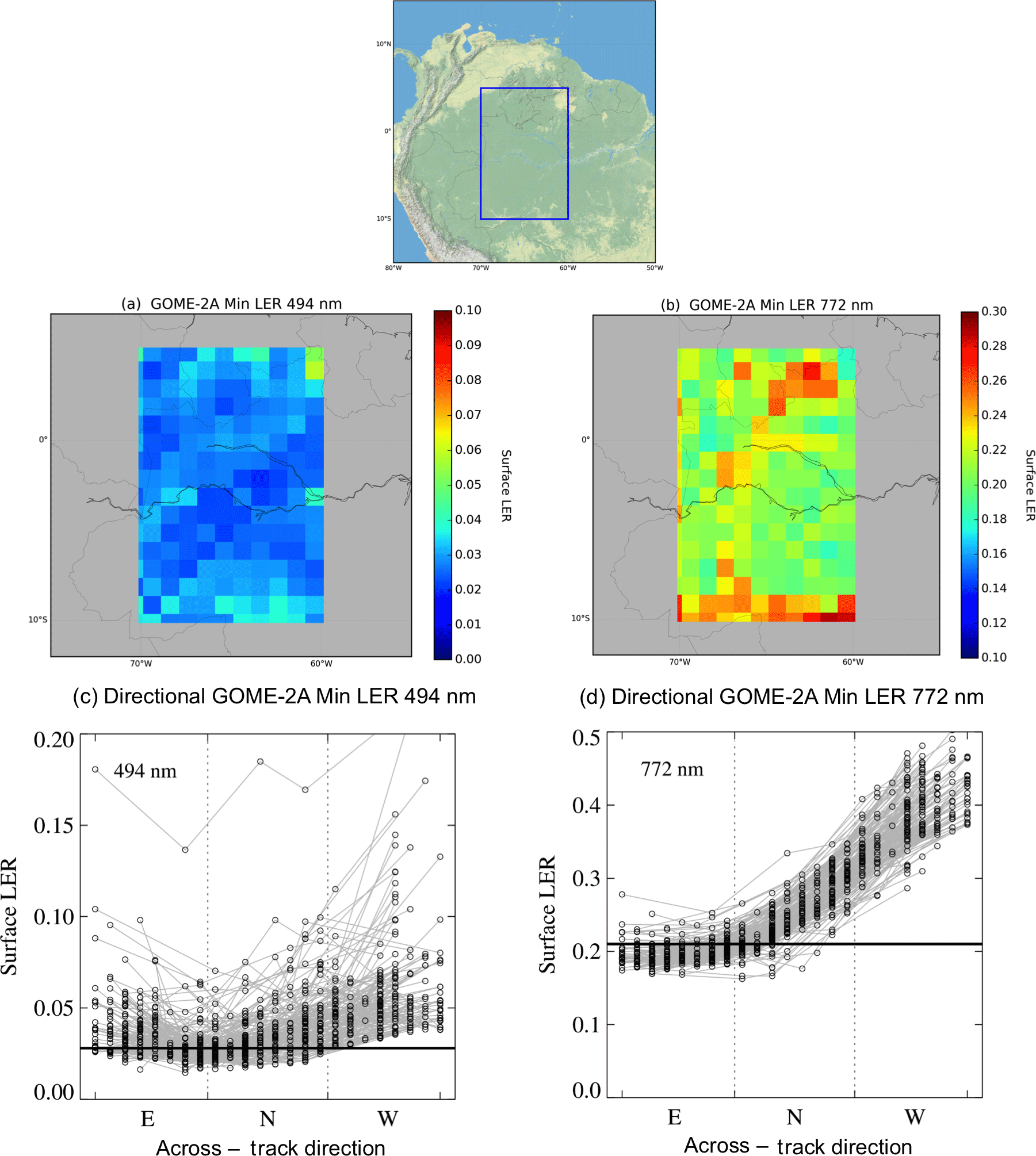
Figure 1(a, b) Map of GOME-2A minimum surface LER climatology (2007–2013) for March (a) at 494 nm and (b) at 772 nm over Amazonia (lat: 5∘ N–10∘ S, long: 60–70∘ W, upper panel) at resolution. (c, d) Directional dependence of surface LER climatology (2007–2013) derived from individual measurements along the swath: east (E) for the eight easternmost pixels, nadir (N) for the eight centre pixels and west (W) for the eight westernmost pixels. The horizontal line represents the surface LER using the full swath which is the average of the surface LER in panels (a) and (b).
Figure 1a, b show the minimum surface LER climatology (2007–2013) at 494 and 772 nm for March over Amazonia for GOME-2 on-board MetOp-A (hereafter GOME-2A) from Tilstra et al. (2017). This climatology was derived from the 1 % cumulative reflectances gathered irrespective of viewing geometry. Figure 1c, d show the directional dependence of the minimum surface LER climatologies derived using the same GOME-2A measurements but now discriminating between different geometries. For this purpose, the 24 measurements in 24 different viewing directions along the GOME-2 swath are considered independently, and then the minimum LER method is applied for each viewing direction as in the derivation of the original full swath climatology. We consider east as the eight most eastward measurements, nadir as the centred ones and west as the eight most westward measurements. The average relative azimuth angle (RAA) characterises the light-scattering regime for measurements in each region: low RAA in the east (RAA = 16∘) corresponds to forward scattering and high RAA (RAA = 164∘) in the west corresponds to backward scattering.
In Fig. 1c, d the horizontal line is the original surface LER value obtained using all GOME-2A measurements over Amazonia, and corresponds to the average value over the box in Fig. 1a, b ( at 494 nm and at 758 nm). The albedo is lower at 494 nm because of the absorption of light by chlorophyll. At 758 nm, if only measurements of the eastern part (E) of the orbit are used to construct the climatology, the average surface LER value is slightly lower () than the value using all measurements. If only nadir (N) measurements are used, the average surface LER increases (), and for the westernmost measurements (W), the average surface LER increases to almost twice the original value (). Using the full swath climatology thus implies a slight overestimation of the surface reflectance for the eastern measurements and a strong underestimation for nadir and western measurements. This systematic effect is a consequence of the directional signature of the surface reflectance. In the backward-scattering direction, canopy surfaces generally appear brighter than in the forward-scattering direction (e.g. Camacho-de Coca et al., 2004). This effect is strongest in the near-infrared (NIR, 0.7–2.5 µm) spectral range, where the atmosphere is more transparent, and over vegetation, which has non-isotropic elements (e.g. dense trees with heterogeneous leave orientation and shadowing effects). The effect in the surface LER climatologies also appears over non-vegetated regions and at shorter wavelengths. However, it is not as strong because stronger Rayleigh scattering tends to smooth out the sensitivity to surface effects and because land surfaces are darker at shorter wavelengths. Non-vegetated areas are usually more isotropic than vegetated areas. Because these biased surface LER climatologies are used in cloud retrievals (e.g. FRESCO Wang et al., 2008, O2–O2 Veefkind et al., 2016), we anticipate a substantial effect on the retrieved cloud properties and as a consequence on trace gas column retrievals that use cloud parameters retrieved in the NIR, where sensitivity to surface anisotropy is strong (such as GOME-2).
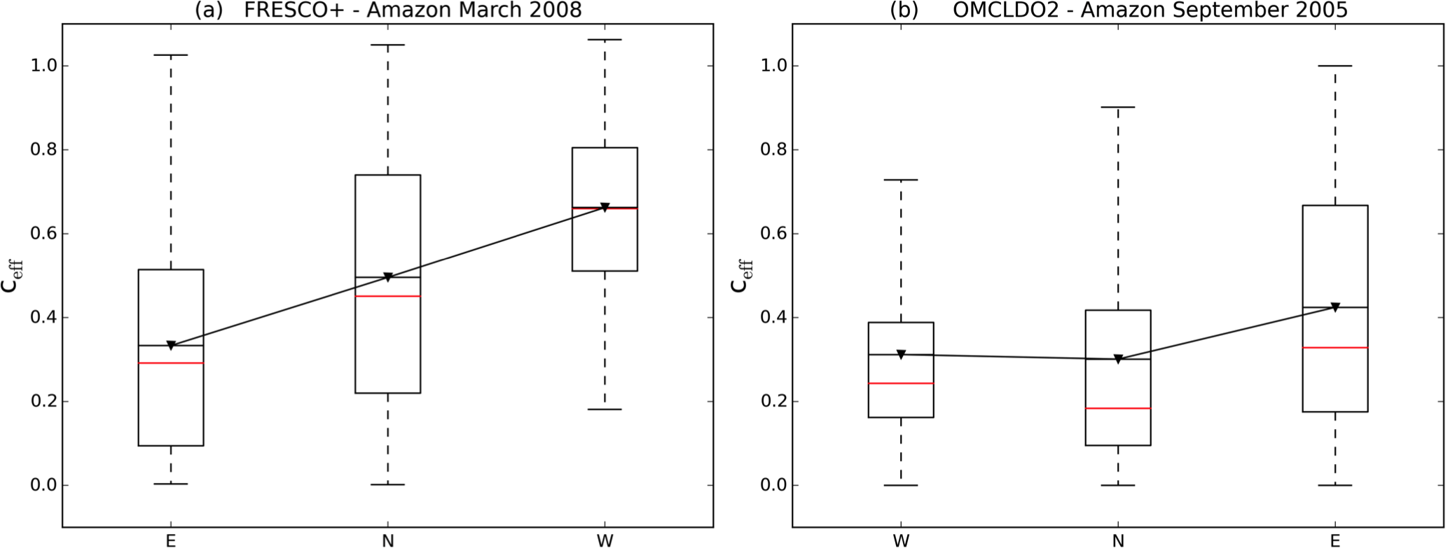
Figure 2Box plot of cloud fractions retrieved with (a) FRESCO cloud retrieval for GOME-2A for March 2008 and (b) OMCLDO2 cloud retrieval for OMI for September 2005 for east–nadir–west measurements over Amazonia (lat: 5∘ N–10∘ S, long: 60–70∘ W). Black triangles correspond to mean values, red lines to median. The box represents 25th and 75th percentiles and the dashed lines the minimum and maximum values.
Indeed, we find that cloud fractions retrieved with FRESCO cloud retrieval from GOME-2 measurements are affected by the across-track bias in the surface LER climatology. FRESCO retrieves cloud properties in the O2 A-band near 760 nm. Figure 2a shows that over Amazonia (in March 2008) FRESCO cloud fractions are generally lower for the eastern measurements than for nadir and western measurements. This dependency can be explained by the directional biases in the surface LER (Fig. 1d). In the nadir and west measurements, the surface LER is underestimated and the retrieval compensates these overestimating cloud fractions in order to match observed TOA reflectances.
This results in higher mean effective cloud fractions for the nadir () and west () measurements compared to the east measurements (). The east–west bias () in the cloud fraction depends on the time of the year and the location. It is not only present over forested areas (i.e. Amazonia (50 %), Equatorial Africa (42 %) in March 2008) but also occurs over other regions (e.g. over Europe (25 %) and Asia (10 %), not shown). Furthermore, in the ensemble of western measurements in most of the regions there are very few cloud fraction values lower than 0.2. This directly impacts trace gas retrievals, because a cloud fraction of 0.2 is often used as a threshold above which it is considered difficult to retrieve tropospheric NO2 columns (cloud screening effect). This bias in FRESCO cloud fractions is significantly higher than the cloud fraction retrieval uncertainty estimates of 0.05 due to surface albedo uncertainty (Koelemeijer et al., 2002), which underlines the need to correct for surface BRDF effects in cloud retrievals in the O2-A band.
The OMCLDO2 cloud retrieval from the OMI retrieves cloud properties in the O2–O2 band around 470 nm and uses the Kleipool et al. (2008) surface LER climatology, which is based on the same principles as the climatology used in FRESCO. Cloud fractions from the OMI instrument retrieved with the OMCLDO2 algorithm also show a west–east1 bias (Fig. 2b) over Amazonia (September 2005) of 26 % (, ) and around 15 % over other regions. The effect is weaker than for GOME-2A (50 % vs. 26 % over Amazonia) but still substantial. The bias shown here is slightly higher than the cloud fraction retrieval uncertainty estimate, which is always below 0.1 (Acarreta et al., 2004), suggesting that the bias in the O2–O2 retrieved cloud fractions can be significant depending on location and time of the year. Because OMI angles are larger than for GOME-2, a larger effect could be expected if the O2-A band was also used to retrieve clouds from OMI measurements.
We have shown that surface BRDF effects result in a distinct across-track bias in surface LER climatologies and cloud fractions retrieved from satellite instruments and that the effect is highly relevant in the NIR and in the visible. Errors in cloud fraction and surface albedo are the most important sources of tropospheric AMF errors (Boersma et al., 2004), so we expect a strong impact on tropospheric NO2 retrievals. In the following section we describe how to account for surface anisotropy in the radiative transfer model DAK. Then, we study how cloud fraction and NO2 AMFs in the framework of cloud and trace gas retrievals are affected by the assumption of a Lambertian surface compared to a realistic anisotropically reflecting surface.
3.1 Definition of BRDF
The amount of radiation reflected by a surface in a certain direction depends on the direction of the incident irradiance and on the direction in which the reflected radiance is observed. The surface bidirectional reflectance distribution function (BRDF) is a function that characterises the directional reflecting properties of a surface. The surface BRDF mathematically describes the angular distribution of the surface reflectance: Rg as a function of the illumination direction (incident, θ′, φ′) and viewing direction (reflected, θ, φ) (see Fig. 3). It is expressed as the ratio of the reflected radiance in a certain direction (dL) and the incident irradiance from a particular direction (dE′) (Nicodemus et al., 1992):
The zenith angle (θ) and the azimuth angle (φ) define the direction of incidence () and reflectance (θ,φ), as sketched in Fig. 3.
The albedo of a surface is generally defined as the ratio of the irradiance reflected by a surface area into the whole hemisphere and the irradiance incident on the surface with hemispherical angular extent (i.e. coming from all directions) (Schaepman-Strub et al., 2006). For particular illumination and viewing conditions, black-sky and white-sky albedo are defined, and they are obtained through hemispherical integration of the surface BRDF. The black-sky albedo is the albedo without diffuse component in the incident irradiance; i.e. the illumination of the surface is from a single direction. It is defined as the integral of the BRDF over the reflection hemisphere of 2π steradian (directional–hemispherical reflectance):
In the particular case when there is only a diffuse isotropic component in the incident irradiance, the white-sky albedo can be defined as the integral of the surface BRDF over both the incident and reflection hemispheres (bihemispherical reflectance):
The blue-sky albedo is a linear combination of Abs and Aws weighted by the fraction of diffuse skylight. The use of either Abs, Aws or ALER in different applications depends on the assumptions of each parameter and the particular application. In the NIR, the diffuse component in the radiation field is much smaller than the direct component so the use of the Abs is justified because it assumes only direct light. Aws might be more suitable for applications in the UV/visible spectral range, where the diffuse component of the incident light may be of comparable size to the direct component. In any case, MODIS visible and NIR Aws and Abs do not differ on average by more than 5 % in summer (Oleson et al., 2003). Aws is constant with solar incident direction, so its use is valid as a ALER but it accounts for some surface BRDF effects (Eq. 3).
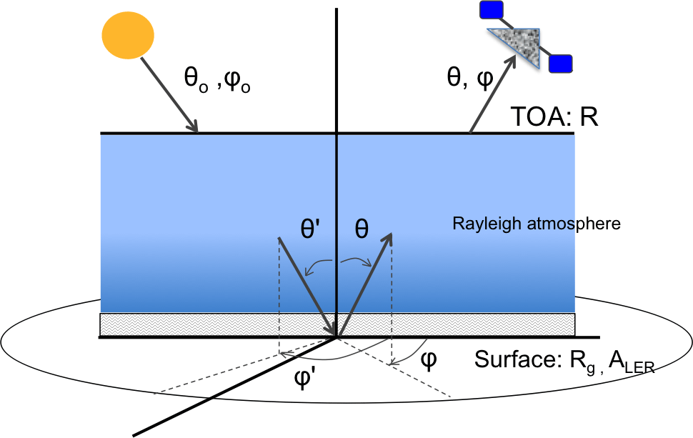
Figure 3Sketch of the surface to top-of-atmosphere system with zenith and azimuth angles that define incident (θ′, φ′) and reflected (θ, φ ) directions of light. Direct incident solar light is described by (θ0, φ0). ALER is the Lambertian surface albedo and Rg the surface BRDF.
Several models have been developed to describe surface BRDF (Wanner et al., 1995). These are either physical, empirical, or semi-empirical models. Physical models are constructed using the laws of physics to explicitly describe the processes that lead to the anisotropic behaviour of surface reflectance. Empirical models characterise the BRDF using mathematical functions that are suitable to describe the observed surface reflectance. Semi-empirical models describe the surface BRDF as a weighted sum of empirical functions derived from physical approximations.
Semi-empirical models are commonly used for global surface BRDF characterisation using remote sensing instruments. In these models, surface reflectance is represented as a linear combination of different terms (the kernels) that characterise different types of scattering that lead to the directional signatures on the reflectance (Roujean et al., 1992). Typically these terms consist of an isotropic term, a volume scattering term, and a geometric scattering term. The weights of the kernels cannot be directly interpreted as physical characteristics from the reflecting surface but just as a first-order approximation of the structure of the surface BRDF (Gao et al., 2003).
In the semi-empirical BRDF Ross Thick – Li Sparse (hereinafter Ross–Li) kernel-driven model, the surface reflectance is expressed as the sum of an isotropic term and two kernels (Ki) that depend on incident zenith angle (θ′), viewing zenith angle (θ), and relative azimuth angle ():
In Eq. (4) Ki are the kernels from the semi-empirical Ross–Li model that describe the three basic scattering types and fi are the surface BRDF parameters that are retrieved from surface reflectance observations from satellite measurements (e.g. MODIS). The surface reflectance cloud-free observations used to obtain the surface BRDF parameters are corrected for absorption and scattering by atmospheric gases, aerosols, and thin clouds (Vermote et al., 1997). Improvements in the atmospheric correction scheme include as much information as possible derived from the satellite itself (e.g. MODIS aerosol optical thickness) (Vermote and Kotchenova, 2008).
The isotropy parameter (fiso) represents the isotropic scattering from a nadir incident and nadir view position. The volumetric scattering is represented by the Ross-Thick kernel, Kvol. It is derived in a single-scattering approximation from radiative transfer theory for a thick homogeneous layer of small scatterers, with equal reflectance and transmittance (Roujean et al., 1992). To account for the reflectance peak in the backward-scattering direction (i.e. the hotspot effect), we include the modification on the volumetric kernel by Maignan et al. (2004). The geometric scattering is represented by the Li–Sparse kernel, Kgeo. For this case, the scene is assumed to contain sparse objects that cast perfectly black shadows with sunlit and shaded portions of the ground and crown contributing to the modelled reflectance of the scene (Li and Strahler, 1986). The exact formulae for these kernels are summarised in Appendix A.
3.2 Surface BRDF implementation in DAK
The radiative transfer model DAK (Doubling–Adding KNMI, Lorente et al., 2017; Stammes et al., 1989; de Haan et al., 1987) is used in the GOME-2 and OMI cloud retrievals (FRESCO and OMCLDO2) and in the DOMINO NO2 retrieval. Originally DAK only considered Lambertian surfaces. To account for the surface reflectance anisotropy in DAK, we have implemented the Ross–Li kernel-driven model. We chose this model for consistency with the retrieval algorithm of the MODIS BRDF/albedo product that we will use in our simulations. The MODIS satellite provides a reliable surface BRDF product and its resolution is suitable to capture surface anisotropy variations for OMI and GOME-2 resolution. MODIS BRDF/albedo products have been successfully used in different fields of atmospheric and climate science such as analysis of radiative forcing due to vegetation change (Myhre et al., 2005) and assessment of land surface albedo in global climate models (Oleson et al., 2003).
After the implementation of the Ross–Li surface BRDF model in DAK, the surface reflectance matrix Rg now contains the full reflection properties of the surface and substitutes the constant isotropic value used for the Lambertian case. This matrix is filled with the surface reflectance calculated with the Ross–Li BRDF model via Eq. (4) as a function of for a specific . For the Lambertian case, the matrix only contains the (1,1) element, which is the value of the surface albedo. We neglect polarisation in the BRDF. In the Doubling–Adding method for radiative transfer calculation, all the matrices (scattering, reflection, and transmission matrices) are expanded in a Fourier series for the integration over following the approach in de Haan et al. (1987). For each Fourier term the Doubling–Adding procedure is applied separately, including the addition of the surface. The mth Fourier coefficient matrix for the surface reflectance matrix is obtained from the relation:
where μ, μ′ are the cosines of the zenith angles in the scattered and incident direction () respectively and is the difference between the scattered and incident azimuth angles.
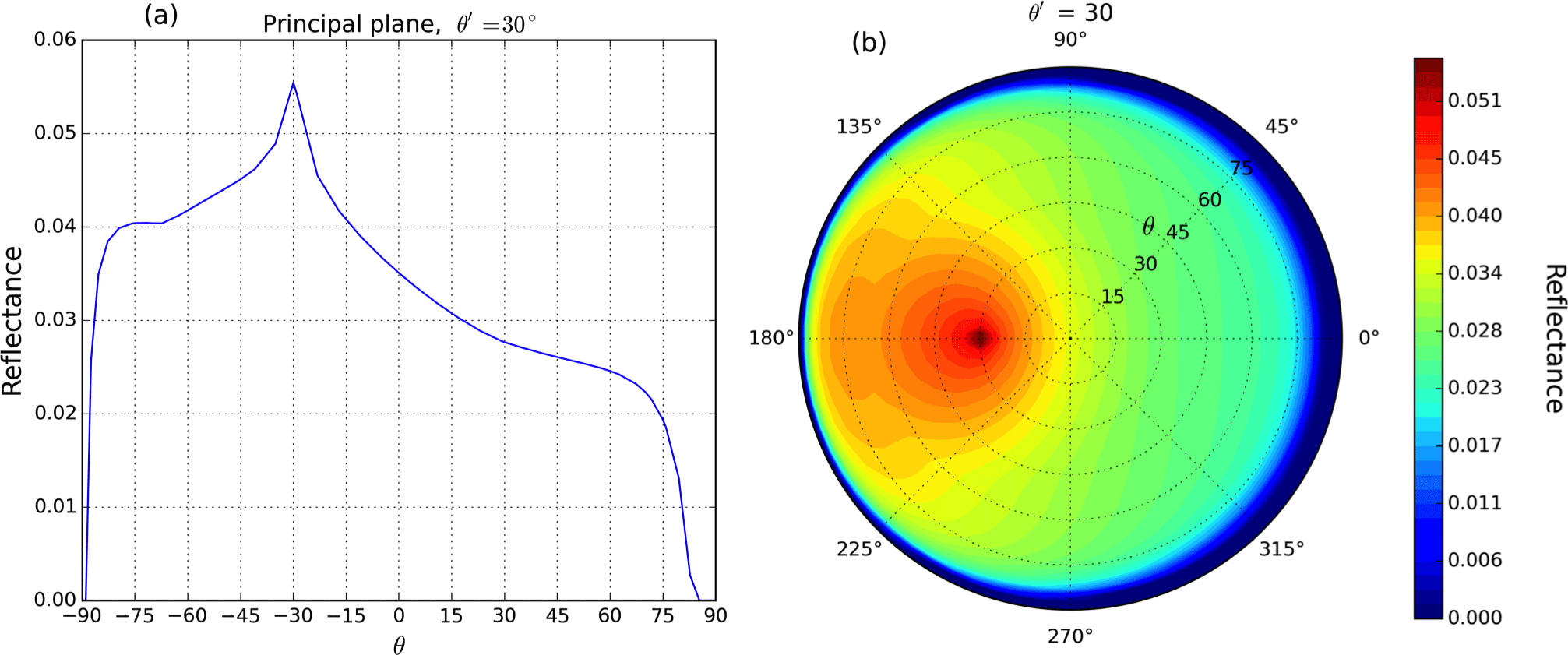
Figure 4Surface reflectance modelled with the Ross–Li surface BRDF model with parameters from MODIS band 3 (459–479 nm) representing a vegetated surface over Amazonia (a) as function of viewing zenith angle in the principal plane ( for negative θ and for positive θ) and (b) in a polar plot with along the azimuth axis and θ along the polar axis for .
The coefficients of the Fourier expansion (Eq. 5) are calculated with the Gauss–Legendre quadrature integration method. It is possible to apply this method because the surface reflection matrix Rg is known at a certain number of division points . The number of Fourier terms (m) and Gaussian points for azimuth () integration needed to resolve the surface BRDF shape depends on the illumination and viewing geometry. For geometries close to the hotspot region in the backward-scattering direction, the number of Fourier terms and Gaussian points needed to reproduce the original BRDF increases significantly with respect to geometries outside the hotspot. In order to reach an accuracy of 10−3 (difference between the original BRDF and the reconstructed BRDF with the Fourier expansion) over the hotspot region, 720 Gaussian points are needed for the azimuth integration, and 300 Fourier terms. Outside the hotspot region, using 60 Gaussian points and 30 Fourier terms in DAK reproduces the original surface reflectance values with an accuracy higher than 10−5. In the final implementation of the surface BRDF in the DAK RTM and in order to have an optimal simulation time, we used 100 Fourier terms and 360 Gaussian points for , also over the hotspot. The overall accuracy obtained with these numbers is within the errors of the radiative transfer modelling for application in satellite retrievals (Lorente et al., 2017).
One of the disadvantages of empirical models is that they depend on observations to derive the parameters fi that describe the surface BRDF. Kernel-based semi-empirical models like the Ross–Li model implemented in DAK only describe the surface reflection accurately for the range of illumination and viewing geometries of the measurements from which they have been derived (Litvinov et al., 2011). The geometries for which the semi-empirical models are valid are thus limited by extreme geometries of instruments like MODIS, which are typically 60–70∘ for θ and θ′. This limit overlaps well with the θ, θ′ values in OMI and GOME-2 measurements for which clouds and trace gas columns are retrieved. For geometries outside the range of MODIS measurement geometries, surface reflectance variations need to be extrapolated.
In radiative transfer modelling with the Doubling–Adding method, in order to calculate the radiation field correctly, the reflectance and transmittance values are needed for all between 0 and 90∘ to be integrated over the complete hemisphere. However, after implementing the Ross–Li BRDF model in DAK, surface reflectance was negative or too high for some combinations of extreme geometries. In order to avoid these unphysical values, we tried various ways of extrapolating values from valid (MODIS-range) angles to the more extreme angles. The different methods did not affect TOA reflectance and albedo values by more than 1 %. Finally, we constrained the surface reflectance to the range [0,1] as in Eq. (6). This is reasonable as negative surface reflectance values are not physically valid, and in nature, surfaces with reflectance higher than 1 do not usually occur (except for surfaces covered by snow or ice). Therefore,
Figure 4 is an example of the surface reflectance computed with the Ross–Li BRDF model for a surface with parameters (fiso, fvol, . This combination of fi values are the spatially averaged parameters from MODIS (BRDF/albedo product MCD43A1) band 3 (459–479 nm) over Amazonia (lat: 5∘ N–10∘ S, long: 60–70∘ W) for March 2008. This representation of a vegetated surface will be used in all the simulations in Sect. 3. The backward-scattering direction corresponds to values of in the polar plot (Fig. 4b) and negative values of θ in the principal plane plot (Fig. 4a). In the backward-scattering direction, the surface reflectance is 2 times higher than in the forward-scattering direction ( in Fig. 4b and positive θ in Fig. 4a). In the backward-scattering direction the hotspot is clearly visible when .
The surface reflectance dependence on geometry as shown in Fig. 4 does not exist when a constant isotropic albedo or surface LER is used. Using a constant albedo for this surface of 0.03 (the equivalent Aws is 0.034) means that in the backward-scattering direction the surface reflectance is underestimated. On the contrary, in the forward direction the surface reflectance is overestimated if an isotropic surface albedo is used. This surface reflectance difference between forward–backward-scattering direction, thus qualitatively explains the east–west bias in the surface LER in Fig. 1. West measurements in GOME-2 correspond to the backward-scattering direction, and for this direction the surface reflectance is higher than in the forward-scattering direction, i.e. east measurement in GOME-2. How this affects effective cloud fractions and NO2 AMFs from GOME-2 and OMI will be analysed in Sect. 4.
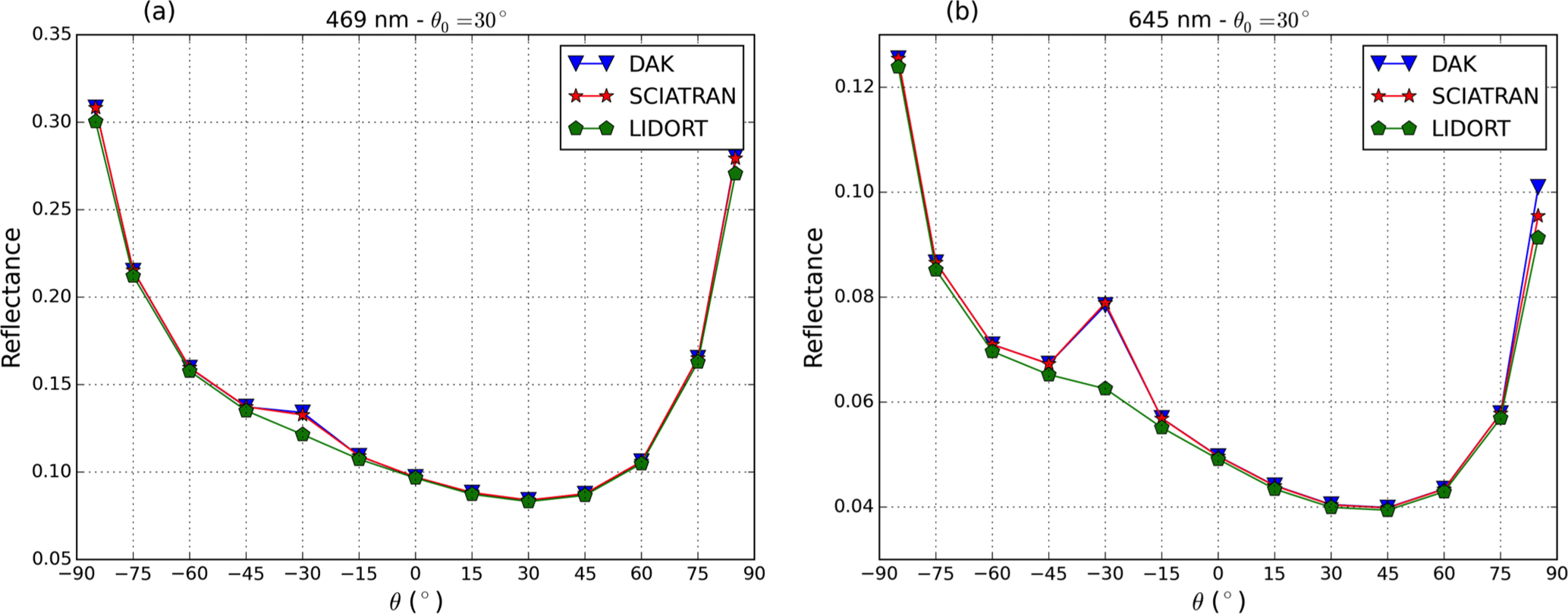
Figure 5TOA reflectance at (a) 469 nm and (b) 645 nm simulated by DAK (blue), SCIATRAN (red), and LIDORT (green) with the Ross–Li surface BRDF model with parameters representing a vegetated surface over Amazonia as in Fig. 4 as a function of the viewing zenith angle in the principal plane ( for negative θ and for positive θ), for .
3.3 Evaluation of surface BRDF effects in DAK TOA reflectances
To evaluate the surface BRDF implementation in DAK we compare TOA reflectances with those simulated by other state-of-the-art radiative transfer models that include a description of surface BRDF effects. Both SCIATRAN (Rozanov et al., 2014) and LIDORT (Spurr, 2004) model the surface reflectance using the Ross–Li model. To minimise the differences due to factors other than the surface BRDF implementations itself, the settings of the three RTMs were as similar as possible. These settings include no polarisation, a plane-parallel standard midlatitude atmosphere and absorption by O3, O2–O2, and NO2.
We select two combinations of the Ross–Li BRDF parameters to model surface reflectance of different surfaces. We simulate TOA reflectances at two different wavelengths: 469 and 645 nm. These wavelengths correspond to the middle of the MODIS band 3 (459–479 nm) and band 1 (620–670 nm) respectively.
Figure 5 shows the simulated TOA reflectance by DAK, SCIATRAN and LIDORT as a function of VZA along the principal plane at 469 and 645 nm. The agreement between the models is within 0.5 % for geometries outside the hotspot region, and DAK and SCIATRAN agree within 1 % over the hotspot. With this simple validation we ensure that our surface BRDF implementation in DAK is correct. The viewing geometry dependency of the TOA reflectance is the effect of Rayleigh scattering of a clean atmosphere. By comparing Fig. 4a with Fig. 5 we see that the effect of surface reflectance anisotropy is dampened by scattering in the atmosphere but the hotspot effect is still visible at both wavelengths after the radiation has passed through the atmosphere. Figure 5 also shows that the hotspot effect is less prominent in TOA reflectance at 469 nm compared to 645 nm, where the atmosphere is more transparent. At 469 nm Rayleigh scattering is stronger than at 645 nm, reducing the effects of surface anisotropy on the TOA reflectance.
We now compare TOA reflectance simulated with surface BRDF and TOA reflectance simulated assuming a Lambertian surface at 469 nm (Fig. 6a, b) and 758 nm (Fig. 6c, d). For simulations at 758 nm we use surface BRDF parameters from MODIS band 2 (841–876 nm) to account for the increase in surface reflectivity near 700 nm (the red edge, e.g. Tilstra et al., 2017). To test the representativeness of band 2 at 758 nm, we scaled the parameters from band 3 (459–479 nm) using the ratio of reflectance at 772 and 469 nm, and the differences with the parameters from MODIS band 2 were negligible. For the Lambertian case, we use the equivalent Aws calculated using the surface BRDF model with Eq. (3). Figure 6b shows that, at 469 nm, the highest absolute differences are around the hotspot region in the backward-scattering direction, where TOA reflectance with BRDF is up to 15 % higher than the TOA reflectance for the Lambertian case. In the forward-scattering direction, TOA reflectance with surface BRDF is 7 % lower than for the Lambertian surface. At 758 nm the effect of surface reflectance anisotropy is much stronger than at 469 nm (Fig. 6c). The highest absolute differences at 758 nm (Fig. 6d) are in the hotspot region in the backward-scattering direction (up to 30 %) and for very extreme angles () in the forward-scattering direction.
These results are consistent with those shown in Figs. 1 and 2: for GOME-2A west measurements (backward-scattering direction), TOA reflectances with surface BRDF are higher than for the Lambertian surface. If these differences are not accounted for in the cloud retrieval, cloud fractions will be biased high in the west measurements to match the measured TOA reflectance. For east measurements in the forward-scattering direction, TOA reflectance with surface BRDF is lower than for the Lambertian surface. Cloud fractions retrieved with surface LER will be biased low to match the measured TOA reflectance. Results from Fig. 6 underline that surface BRDF effects in retrieved cloud fractions are stronger for FRESCO at 758 nm than for OMCLDO2 at 477 nm. Our results also show that the error in TOA reflectances due to the use of a Lambertian albedo is substantial, but its magnitude is highly dependent on the spectral and geometrical characteristics of the measurements: effects are stronger at 758 nm and around the hotspot region in the backward-scattering direction.
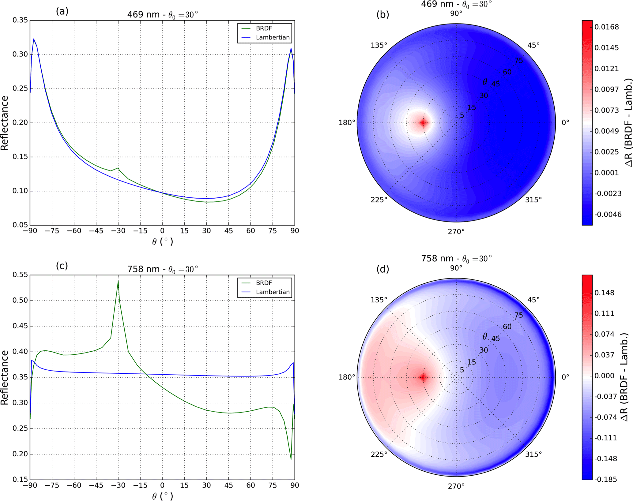
Figure 6(a, c) TOA reflectance as a function of viewing zenith angle simulated by DAK at 469 and 758 nm with a Lambertian surface (blue line) and with surface BRDF (green line) in the principal plane ( for negative θ and for positive θ). (b, d) Absolute differences between TOA reflectance with surface BRDF and with a Lambertian surface at 469 and 758 nm. Surface BRDF parameters represent a vegetated surface over Amazonia at 469 nm (fiso, fvol, and 758 nm (fiso, fvol, . Note the different scales.
4.1 Synthetic cloud fraction retrieval
In Sect. 2 we showed that there is an east–west bias in the retrieved cloud fractions from GOME-2 and OMI. Effective cloud fractions in FRESCO and OMCLDO2 are retrieved as follows (Stammes et al., 2008; Veefkind et al., 2016):
Rmeas is the TOA reflectance measured by the satellite instrument, Rcr is the simulated clear-sky TOA reflectance, and Rcd is the simulated cloudy-sky TOA reflectance assuming that the cloud is a Lambertian reflector with a fixed albedo of 0.8. In the current versions of FRESCO (v7) and OMCLDO2 (v2.0) cloud retrievals, the simulated clear-sky TOA reflectances in Eq. (7) assume that the surface is Lambertian. Due to this assumption, any surface anisotropy signal in the measured TOA reflectance (Rmeas) is neglected and, consequently, ends up in the retrieved effective cloud fraction.
Table 1Settings for Lambertian and BRDF ceff simulations in Sect. 4.1. Inverse model for Lambertian ceff reproduces current O2–O2 and FRESCO+ retrievals, with Lambertian surface and Lambertian cloud. Inverse model for BRDF ceff reproduces the retrieval accounting for surface BRDF effects.
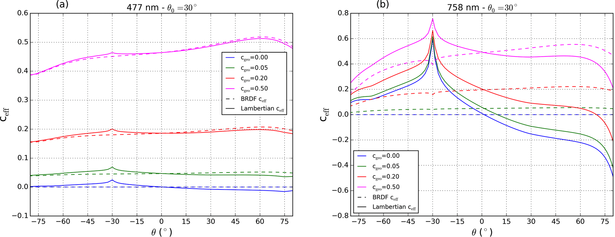
Figure 7Simulated effective cloud fraction at (a) 477 nm and (b) 758 nm as a function of viewing zenith angle for different geometric cloud fractions along the principal plane ( for negative θ and for positive θ). and cgeo=0, 0.05, 0.2, and 0.5. At 477 nm: BRDF parameters (solid line) (fiso, fvol, and for Lambertian surface Aws=0.0217 (dashed line). At 758 nm: BRDF parameters (solid line) (fiso, fvol, and for Lambertian surface Aws=0.337 (dashed line).
To improve our understanding of how surface reflectance anisotropy influences the retrieval of cloud fractions, we use the forward model DAK to approximate Rmeas by simulating the TOA reflectance for a scene with a Henyey–Greenstein cloud and surface reflectance anisotropy. This resembles what the satellite would measure in a realistic cloudy scene. We express Rmeas as the sum of TOA reflectance of the cloudy and the clear parts of the scene, weighted by a geometric cloud fraction cgeo (independent pixel approximation):
The effective cloud fraction is the part of the pixel that the Lambertian cloud has to occupy to match the observed reflectance. The geometric cloud fraction is the part of the pixel that is covered by the “true” cloud (Stammes et al., 2008).
The settings of the simulations are summarised in Table 1. We simulate TOA reflectances and cloud fractions in the spectral regions where cloud fractions are calculated in the cloud algorithms. The Ross–Li BRDF parameters are from a climatology created by the QA4ECV Land Group at the Mullard Space Science Laboratory (University College London). This data set consists of daily BRDF parameters collected from 16 years of MODIS measurements (Strahler et al., 1999; MCD43A1, 2015) from 2000 to 2016 (QA4ECV-WP4, 2016). Parameters from band 3 (459–479 nm) are representative for simulations in the O2–O2 absorption band and parameters from band 2 (841–876 nm) for simulations in the O2–A band (see Sect. 3.2). Monthly averaged parameters from this data set over Amazonia are shown in Figs. S2, S3 in the Supplement.
We calculate cloud fractions using Eq. (7) with Rcr simulated with a Lambertian surface consistent with the current O2–O2 and FRESCO+ retrievals (hereafter Lambertian ceff) and by accounting for surface BRDF effects (hereafter BRDF ceff). The Lambertian cloud is located at the same pressure level as the Henyey–Greenstein cloud so we can isolate surface BRDF effects on cloud fraction only (see settings in Table 1).
Figure 7 shows that cloud fractions accounting for surface BRDF effects (dashed lines) depend only weakly on geometry, whereas cloud fractions with a Lambertian surface (solid lines) are higher in the backward-scattering direction, at both 477 and 758 nm and especially for the lowest cgeo. At 758 nm this is true even for a geometric cloud fraction as high as 0.5. In the backward-scattering direction, surface reflectance is higher than reflectance by a Lambertian surface. Therefore clear-sky TOA reflectance with a Lambertian surface cannot explain the higher-simulated reflectance in Eq. (7), which results in high Lambertian ceff.
Surface BRDF effects are more important for small cloud fractions, and less importance for large cloud fractions. For cloudy pixels the effect of surface reflectance anisotropy vanishes because the scattering by the cloud dominates in the measured reflectance. Figure 7 shows that for large cgeo, the viewing zenith angle dependency of the effective cloud fractions is due to the Henyey–Greenstein scattering cloud, which gives relatively higher scattering in the forward direction.
At 477 nm, surface BRDF effects on cloud fractions are less evident than at 758 nm. In the visible spectral region, surface BRDF effects are suppressed by Rayleigh scattering smoothing out the surface anisotropy effects on TOA reflectances. For lower geometric cloud fraction, Lambertian cloud fractions are moderately higher (by 0.05) in the backward-scattering direction than in the forward-scattering direction. These findings underscore the relevance of accounting for surface BRDF effects because measurements with small cloud fractions are most sensitive to pollution in the lower troposphere.
Differences in Lambertian cloud fractions between backward- and forward-scattering directions at 758 nm are on average 0.35. At 477 nm, the differences amount to 0.1, depending on the surface and the geometry. This is consistent with the observed bias in FRESCO and OMCLDO2 cloud fractions shown in Fig. 2. The absence of a backward–forward-scattering dependency in the BRDF ceff implies that accounting for surface BRDF effects will reduce the east–west across-track bias in retrieved cloud fractions.
4.2 GOME-2A cloud fraction simulations
We simulate Lambertian and BRDF cloud fractions for GOME-2A measurements over Amazonia in March 2008. We use the exact illumination and viewing geometry (θ,θ0, φ−φ0) of each individual measurement and co-locate MODIS pixels with the GOME-2A pixel centre to obtain the surface BRDF parameters over the scene. For Lambertian cloud fractions, we use the GOME-2A surface LER value from Tilstra et al. (2017). To simulate the measured reflectance, we assume a geometric cloud fraction distribution with an area-wide average of . Figure 8a, d show the distribution for east and west measurements respectively.
Figure 8 shows simulated Lambertian (panels b, e) and BRDF (panels c, f) effective cloud fractions for east and west GOME-2A measurements. For east measurements, both Lambertian () and BRDF () cloud fraction simulations capture the original geometric cloud fraction distribution and absolute values. This means that surface BRDF effects are weaker in the east, consistent with the smaller surface LER climatology bias for measurements on the east part of the orbit (Fig. 1). For west measurements, the original distribution is reproduced well in the BRDF cloud fractions (), but the Lambertian values show a significant overestimation (). A box plot of these distributions is shown in Fig. S4 in the Supplement. The east–west bias in the Lambertian simulation (0.2) is considerably reduced (0.01) for the BRDF cloud fractions: the across-track bias in the FRESCO data is a direct consequence of neglecting surface BRDF effects. We conclude that accounting for these surface BRDF effects can largely solve the bias in cloud fractions measured in the backward-scattering regime over Amazonia. Although we have not made an analysis of the surface BRDF effects in a complete retrieval, the biases in cloud fraction found over other regions will probably be reduced after accounting for surface BRDF effects.
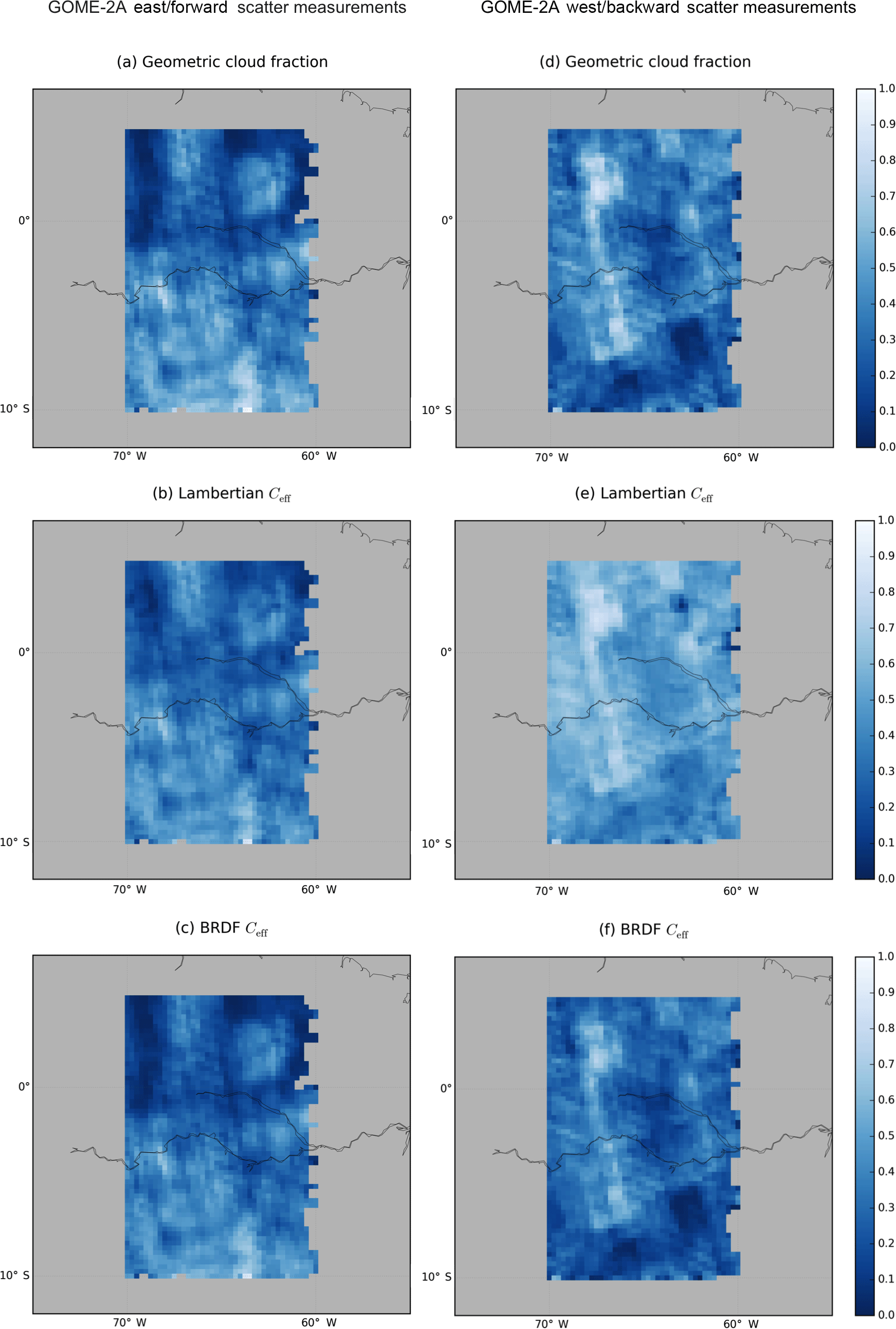
Figure 8Geometric cloud fraction distributions for (a) east and (d) west GOME-2A measurements. (b, e) Lambertian and (c, f) BRDF cloud fraction simulations for east (a–c) and west (d–f) GOME-2A measurements. Plots show averaged cloud fractions in a grid over Amazonia (lat: 5∘ N–10∘ S, long: 60–70∘ W) for March 2008.
Here we investigate the effects of accounting for surface reflectance anisotropy on tropospheric NO2 column retrievals under clear-sky and partly cloudy conditions. We calculate tropospheric AMFs with surface BRDF and with a Lambertian surface, including the surface BRDF effects on retrieved cloud fractions (Sect. 4) for GOME-2A measurements over Amazonia and over France.
In satellite retrievals of trace gases, an air mass factor (M) is used to convert the slant column density (Ns, SCD) from the measured reflectance spectra into the vertical column density (Nv, VCD):
The AMF depends on the surface reflectance (Rs), surface pressure (Ps), cloud fraction, and pressure (fcd,Pcd), a priori NO2 profile (xa) and measurement geometry ().
Here, tropospheric NO2 AMFs are calculated by differencing the logarithm of simulated TOA reflectances with and without trace gas in the troposphere divided by the absorption optical thickness of the gas τgas:
Table 2Settings for the Lambertian and BRDF tropospheric NO2 AMF calculations shown in Fig. 9.
AMF is directly affected by the assumption of a Lambertian surface instead of an anisotropic surface in the simulated TOA reflectance. In addition, AMFs are indirectly affected by the cloud radiance fraction (fcd) used to correct for residual clouds, in which calculation a Lambertian surface is assumed as well. To account for the presence of clouds, we use the independent pixel approximation (IPA; see also Eq. 8), which consists of calculating the total AMF for a partly cloudy scene as a linear combination of cloudy (Mcd) and clear (Mcr) components of the AMF, weighted by the cloud radiance fraction w:
The use of a Lambertian surface thus influences the AMF directly via Mcr and indirectly via w:
where ceff is the cloud fraction, and Rcd and Rcr are the radiances for totally cloudy and clear-sky scenes. Cloud radiance fraction depends on the Lambertian surface assumption via Rcr and ceff.
5.1 BRDF effects on tropospheric NO2 air mass factors
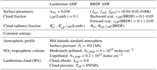
We calculate AMFs with Eq. (10) by simulating TOA reflectances with surface BRDF and with a Lambertian surface. The settings of the simulations are summarised in Table 2. Based on our analysis (Sect. 4.1), we include a change of ±0.05 over the Lambertian cloud fraction with a decrease of −0.05 in the backward-scattering direction and an increase of +0.05 in the forward-scattering direction to quantify how the surface BRDF effects on clouds propagate to the final AMF.
Figure 9a shows surface BRDF effects on Mcr for a moderately polluted troposphere as a function of VZA along the principal plane. In the backward-scattering direction, BRDF Mcr is higher by 5–20 %. The higher surface BRDF reflectance and TOA reflectance makes the retrieval more sensitive to the NO2 in the boundary layer. In the forward-scattering direction, BRDF Mcr is lower by 5–15 %.
Figure 9b shows surface BRDF effects on w and Fig. 9c shows the combined effect on total tropospheric M of changes in Mcr and in w in a partly cloudy scene with a ceff(Lamb.)=0.1. In the backward-scattering direction, tropospheric M is 9–30 % higher when accounting for surface BRDF effects. The decrease in ceff (and hence w) makes the retrieval more sensitive to the NO2 below the cloud. In the forward-scattering direction, tropospheric M is 14 %–22 % lower when accounting for surface BRDF effects because of the stronger screening effect by the higher BRDF ceff. The surface BRDF effect on w enhances the effect on the clear-sky AMF by up to 10 % in both the forward and backward-scattering directions.
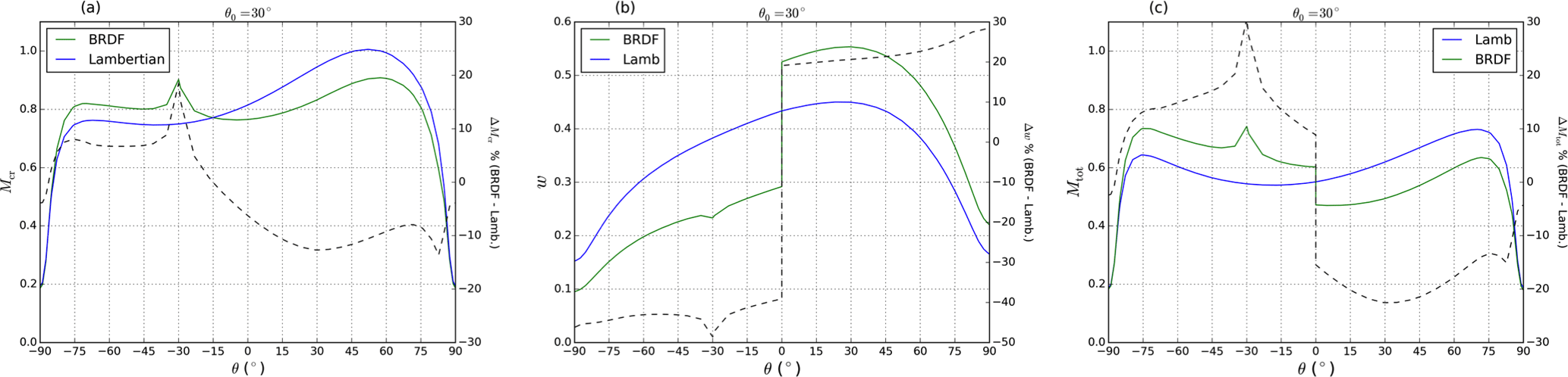
Figure 9(a) Clear-sky tropospheric NO2 AMF, (b) cloud radiance fraction, and (c) total tropospheric NO2 AMF computed with surface BRDF (green) and with a Lambertian surface (blue) and their relative difference (right axis) as a function of viewing zenith angle in the principal plane ( for negative θ and for positive θ), for . Pcd=850 hPa, Lambertian ceff=0.1 and BRDF . Surface BRDF parameters are (fiso, fvol, and Aws=0.036 for the Lambertian surface. Troposphere is moderately polluted ( molec cm−2).
Figure 10 shows surface BRDF effects on total tropospheric M in partly cloudy scenes with increasing cloudiness for the specific combination of (θ, , 30∘) in the principal plane, representative of typical GOME-2 or OMI measurements. For a polluted troposphere (represented by stars), the total effect of accounting for surface BRDF is to increase M in the backward-scattering direction (Fig. 10a) and to reduce M in the forward-scattering direction (Fig. 10b). Average relative differences of about 15 % for Mcr increase up to 25 %–40 % for low cloud fractions (below 0.1) (see Fig. S5 in the Supplement). The effect decreases for higher cloud fractions, with relative differences below 10 % for cloud fractions higher than 0.5. For a lower bias in ceff (e.g. 0.02), the effect on M reduces to about 15 %–20 %, which is still a considerable effect.
For an unpolluted troposphere, surface BRDF effects on Mcr are in the same direction as in the polluted case but smaller (−7 % to +11 %). In a partly cloudy scene, Lambertian and BRDF tropospheric M are similar within −3 % to 7 %. Because there is very little NO2 below the cloud, the effect of a change in w counteracts (and largely cancels) the effect on the clear-sky AMF (circles in Fig. 10).
Figure 10Total tropospheric NO2 AMF as a function of cloud fraction in the (a) backward-scattering direction and (b) forward-scattering direction computed with surface BRDF (green) and a Lambertian surface (blue), for Pcd=850 hPa, (θ, , 30∘), for a moderately polluted (stars) and unpolluted (circles) troposphere. BRDF parameters are (fiso, fvol, and Aws=0.036 for the Lambertian surface.
Figure 11 shows surface BRDF effects on total tropospheric AMF as a function of cloud pressure, for a cloud fraction of 0.1. For cloud pressures higher than the 850 hPa assumed in Fig. 10, the contribution of surface BRDF effects to the change in M from the change in cloud fractions is dampened. There is a range of cloud pressures (in Fig. 11 between 900 and 950 hPa) for which the effects on Mcr and on cloud fraction compensate each other. For an even higher cloud pressure (e.g. 978 hPa), Mcd is larger than Mcr and the sign of the effect changes. In the backward-scattering we have lower BRDF AMFs and in the forward-scattering higher BRDF AMFs. In the unpolluted situations the differences are larger for higher cloud pressures.
Although this study does not address surface BRDF effects on cloud pressure, we did a preliminary analysis, applying a directional surface LER derived from GOME-2 in FRESCO+. The analysis shows that accounting for surface reflectance anisotropy effects reduces the cloud pressure by 40 hPa on average (with differences up to 120 hPa). This high bias in retrieved cloud pressure implies that the results shown for 850 hPa might be representative of the surface BRDF effects on AMFs for clouds currently retrieved at higher (biased) pressures.
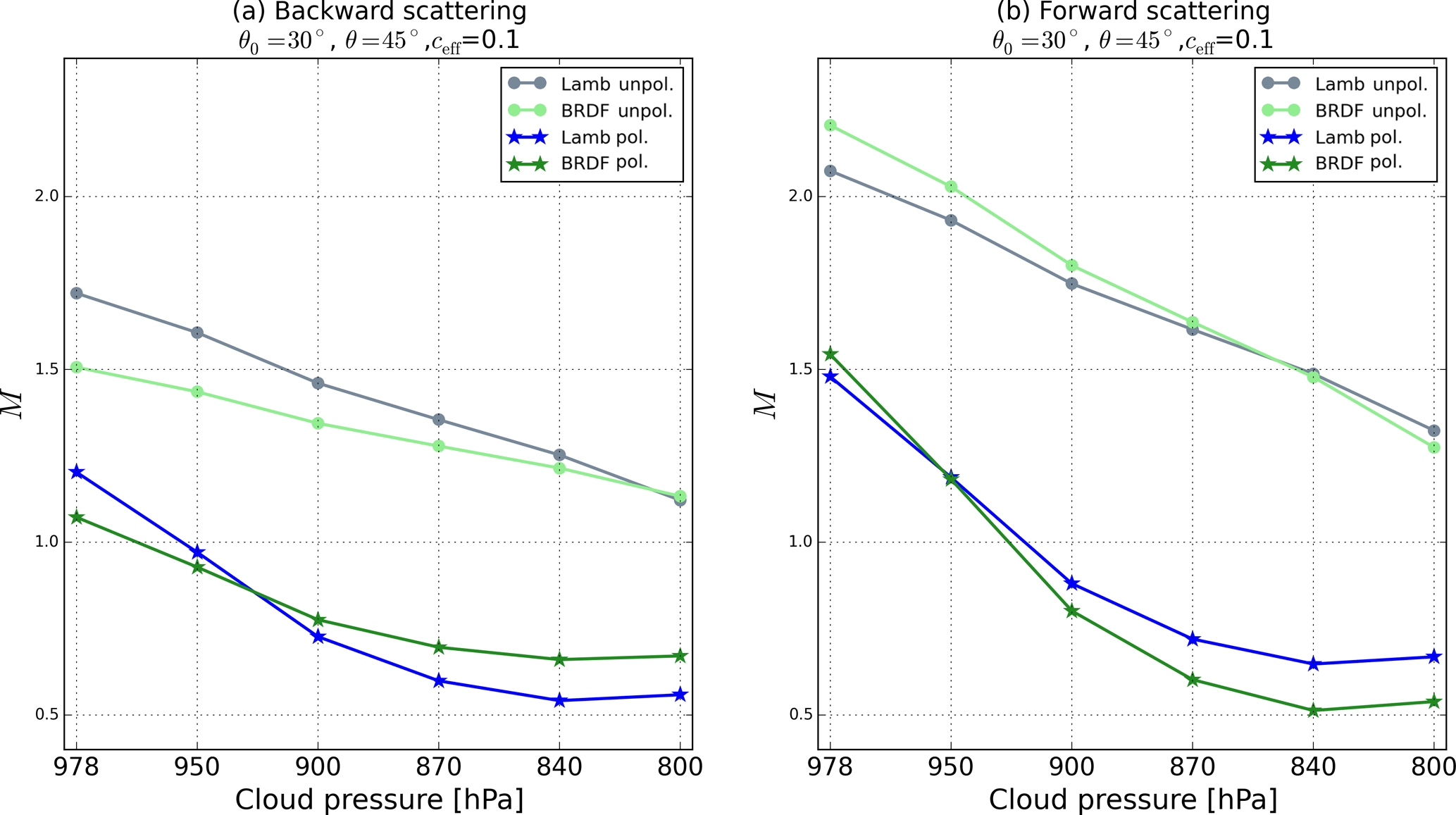
Figure 11Total tropospheric NO2 AMF as a function of cloud fraction in the (a) backward-scattering direction and (b) forward-scattering direction computed with surface BRDF (green) and a Lambertian surface (blue), for Pcd=850 hPa, (θ, , 30∘), for a moderately polluted (stars) and unpolluted (circles) troposphere. BRDF parameters are (fiso, fvol, and Aws=0.036 for the Lambertian surface.
5.2 GOME-2A tropospheric NO2 air mass factors
We calculate Lambertian and BRDF NO2 tropospheric AMFs for the exact illumination and viewing geometries of GOME-2A measurements over Amazonia and over France for March 2008. This results in approximately 1300 clear-sky pixels analysed over Amazonia and 700 over France. We assume a moderately polluted atmosphere in every scene and collocate MODIS pixels with the GOME-2A pixel centre to obtain the surface BRDF parameters. For the Lambertian simulations, we use the surface LER value of each pixel from the GOME-2 climatology. We apply Lambertian and BRDF ceff distributions from Sect. 4.2 (as in Fig. 8). This way we account for the calculated surface BRDF effects in cloud fraction instead of the average change of 0.05 assumed in the sensitivity analysis in Sect. 5.1.
Figure 12a shows that for east measurements (i.e. forward scattering), Mcr decreases on average by 18 % over Amazonia. Over France the decrease is on average 8 % (not shown). Figure 12b shows that for west measurements (i.e. backward scattering), Mcr increases on average 5 % over Amazonia and 7 % over France, consistent with our findings in Fig. 9a. The differences of 15 %–23 % found in this analysis agree with the reported differences of 10 %–20 % in Noguchi et al. (2014) and Zhou et al. (2010) for clear-sky AMFs. The higher BRDF AMFs in the upper-right corner of our study area correspond to a savanna ecosystem that is brighter than the dense rainforest. Because of the higher resolution of the MODIS BRDF data set, this feature is well captured and leads to higher AMFs both in the east and west measurements (see Fig. S2 in the Supplement). MODIS albedo is able to capture spatial variability on scales that satellites with coarser pixels cannot (Russell et al., 2011).
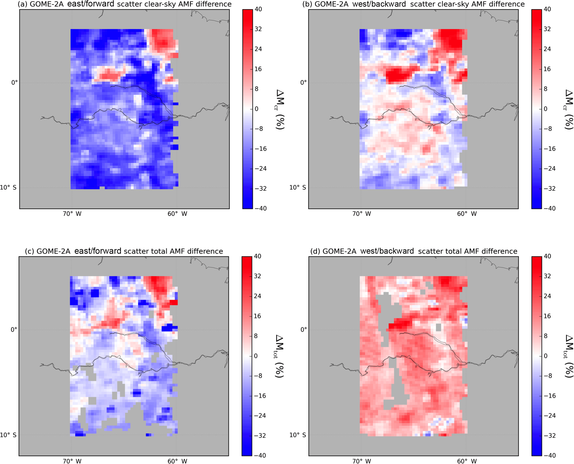
Figure 12Relative differences between BRDF and Lambertian AMFs over Amazonia for March 2008: (a) clear-sky tropospheric NO2 AMFs for east GOME-2A measurements (forward scatter), (b) clear-sky tropospheric NO2 AMFs for west GOME-2A measurements (backward scatter), (c) total tropospheric NO2 AMF for east GOME-2A measurements (forward scatter) and (d) total tropospheric NO2 AMF for west GOME-2A measurements (backward scatter). Total AMFs are only shown for ceff<0.5.
Figure 12c shows that for east measurements (i.e. forward scattering), total tropospheric AMFs including surface BRDF effects on cloud fractions are on average 10 % lower over Amazonia. The decrease is on average 7 % over France (not shown). For west measurements, (i.e. backward scattering), total AMFs are on average 16 % higher over both Amazonia (Fig. 12d) and France, illustrating that the Mcr effect is enhanced by the effect on the cloud fraction by 10 %–15 % on average. Vasilkov et al. (2017) also found increased differences in the tropospheric AMFs due to surface BRDF effects on cloud parameters, but as reported by Lin et al. (2014), there can also be compensating effects.
These results show that surface BRDF affects both clear-sky AMF and cloud radiance fractions, which in combination significantly affect total NO2 AMFs. As shown in Figs. 10–12, the sign and magnitude of the surface BRDF effects show strong spatial variations and depend on cloud fraction and cloud pressure. In order to generalise the effects to a global retrieval, a full assessment including all possible retrieval conditions should be done. Over forested terrain, current tropospheric AMFs are likely underestimated in the backward-scattering regime and overestimated in the forward-scattering regime by up to 25 %–35 %, explained by systematic errors in Mcr and w. These results show that surface BRDF effects have to be included consistently in both cloud and trace gas retrievals.
We analysed the effects of surface reflectance anisotropy on the OMI and GOME-2 satellite retrievals of cloud parameters and tropospheric NO2 columns that currently use Lambertian-equivalent reflectivity (LER) climatologies. These climatologies, and consequently retrieved cloud fractions, show substantial across-track biases over terrain with a strong BRDF directionality. Here we interpret these with the DAK radiative transfer model. A clear understanding of the reasons for the biases and how they propagate in the tropospheric NO2 column retrieval is critical to improve cloud and trace gas retrieval algorithms for satellite sensors.
An important finding is that the LER climatologies slightly overestimate surface albedo for forward-scattering satellite-viewing geometries (eastern part of GOME-2 orbit) and highly underestimate the surface albedo for backward scattering viewing geometries (western part). The underestimation is as large as a factor of 2 over forested scenes in the near-infrared (772 nm). They are weaker but still relevant in the visible (494 nm), where surfaces are darker and Rayleigh scattering effects are stronger. This across-track bias in surface LER propagates into the cloud fraction retrievals: we find biases in cloud fractions of up to 50 % between backward-scattering and forward-scattering geometries in the GOME-2 FRESCO and 26 % in the OMI OMCLDO2 cloud algorithms. Time of day does not drive the importance of surface BRDF effects but specific viewing geometry and spectral range do.
To interpret the above biases, we extended the description of surface reflectance in DAK to include the geometrical surface reflecting properties via the bidirectional reflectance distribution function (BRDF) from the Ross–Li semi-empirical model. This allows DAK to simulate not only isotropic reflection at the surface but also the anisotropic contributions from volumetric (e.g. leaf scattering) and from geometric (e.g. shadow-casting) effects. We evaluated DAK top-of-atmosphere (TOA) reflectance simulations against other radiative transfer models and find agreement within 1 % between DAK and SCIATRAN, even within the hotspot backscatter reflectance peak. We then simulated TOA reflectances over vegetated scenes using BRDF parameters from a daily high-resolution database derived from 16-years of MODIS measurements recently developed within the QA4ECV project (QA4ECV-WP4, 2016). Our updated DAK simulations show considerably higher TOA reflectance levels for backward-scattering viewing geometries than those with isotropic surface reflection (LER) only. This strongly indicates that across-track biases in cloud fractions can be explained by the lack of a description of surface reflectance anisotropy in the FRESCO and OMCLDO2 algorithms.
Subsequent sensitivity tests indicated that accounting for surface reflectance anisotropy in the FRESCO and OMCLDO2 retrieval framework removes the bias in cloud fractions. A correct physical description of surface anisotropy is essential for FRESCO, because cloud properties are retrieved in the NIR spectral range (760–790 nm) where surface BRDF effects are stronger and the atmosphere is virtually transparent. It is also of high relevance for scenes with low cloud fractions, where trace gas retrievals are still sensitive to pollution close to the ground. A discussion on the validity of the Lambertian cloud model is beyond the scope of this study. Nevertheless, the cloud fraction dependency with VZA for cloudy scenes suggests that the use of a more realistic cloud model should be considered in future improvements of cloud retrievals.
The implications for NO2 air mass factor (AMF) calculations are substantial. Total tropospheric NO2 AMFs are calculated as the radiative cloud fraction-weighted sum of cloudy and clear-sky AMFs. For moderately polluted NO2 and backward-scattering geometries, we find that clear-sky AMFs are up to 20 % higher and cloud radiance fractions up to 40 % lower if surface reflectance anisotropic effects are accounted for. The combined effect of these changes (with clouds located at 850 hPa) is that NO2 AMFs in polluted situations increase by 25 %–30 % for backward-scattering geometries (and decrease by 25 %–35 % for forward-scattering geometries), stronger than the effect of either contribution alone.
An issue that was not addressed in this study is the role of aerosols. Noguchi et al. (2014) showed that scattering by aerosols generally dampens surface BRDF effects for clear-sky scenes. However, more research is needed to assess how specific aerosol characteristics (i.e. aerosol amount and type, vertical distribution relative to cloud) will affect cloud parameter retrievals and air mass factor calculations both in clear-sky and cloudy conditions.
We conclude that it is necessary to coherently account for surface reflectance anisotropy effects in retrievals of cloud properties and trace gases from UV/vis satellite sensors. Although this study does not apply surface BRDF to a complete global cloud and NO2 retrieval, it shows that it has substantial effects on both cloud fractions and NO2 AMFs. A number of recent studies have attempted to account for the effects of anisotropic reflectance on both cloud and NO2 retrievals (Lin et al., 2014; Vasilkov et al., 2017), but a global assessment including the full range of possible retrieval conditions is still missing. An additional incentive to account for surface reflectance anisotropy is that the currently available LER climatologies (Kleipool et al., 2008; Tilstra et al., 2017) describe the spatial variation in albedo on a scale (–) coarser than the OMI or GOME-2 pixel itself (13×24 km2/80×40 km2). Using these coarse LER climatologies in AMF calculations degrades the intrinsic spatial resolution of the satellite retrievals, an issue that will be exacerbated for the recently launched TROPOMI instrument, with pixels as small as 3.5×7 km2. A viable alternative to the current LER climatologies is provided by the MODIS-derived BRDF-parameters at a spatial resolution better than the GOME-2, OMI, and TROPOMI pixel sizes. MODIS Terra and Aqua are expected to last until 2025 and afterwards the Joint Polar Satellite System (JPSS) satellite constellation ensures continuity of land observations needed to produce surface BRDF data. Sentinel-3 could be employed to generate a BRDF similar to the one from the ESA GlobAlbedo broadband and the QA4ECV spectral albedo after some years of measurements. Another alternative is to make a directionally dependent LER database from TROPOMI once there is enough surface reflectance data acquired by the satellite itself.
Radiative transfer model DAK is available upon request (contact persons: Piet Stammes and Ping Wang). FRESCO and OMCLDO2 cloud product and OMI DOMINO NO2 product are publicly available and the datasets can be found at http://www.temis.nl/. QA4ECV surface BRDF climatology is available upon request (contact person: Jan-Peter Muller).
We summarise here the expressions of the kernels implemented in DAK to model the surface reflectance anisotropy. We refer the reader to the original literature where these kernels were derived for more detailed information.
A1 Ross-Thick kernel
The expression of the Ross-Thick volumetric scattering kernel is (Roujean et al., 1992):
Here θ′ and θ are the incident and reflected zenith angles respectively. ξ is the scattering angle defined as follows:
where is the relative azimuth angle (reflected and incident azimuth difference).
The term in the second pair of squared bracket in Eq. (A1) is the modified part for the hotspot modelling, where ξ0 is the hotspot characteristic angle (typically 1.5∘). This characteristic angle can be related to the ratio of the size of the scattering element and the canopy vertical density (Maignan et al., 2004).
A2 Li–Sparse kernel
The expression of the Li–Sparse geometric scattering kernel is (Li and Strahler, 1986; Wanner et al., 1995):
The different terms in the equation are as follows:
The angles with a star are equivalent angles to convert spheroid-like object to spheres:
O (Eq. A4) is the overlap area between the shadow of illumination and the shadow of viewing projections on the ground. D is the distance between the centres of the scattering objects. The parameter t is used to parameterise the scattering objects spherically. This kernel it is not linear as it has two parameters and describing the shape and the relative height of the scattering objects, and in the simulations in this study are set to 1 and 2 respectively.
The supplement related to this article is available online at: https://doi.org/10.5194/amt-11-4509-2018-supplement.
The authors declare that they have no conflict of interest.
This research has been supported by the EU FP7 Project Quality Assurance for
Essential Climate Variables (QA4ECV), grant no. 607405. We acknowledge the
free use of the GOME-2 data provided by EUMETSAT.
Edited by: Michel Van Roozendae
Reviewed by:
two anonymous referees
EEA: Air quality in Europe – 2016 Report, Tech. Rep. 28/2016, TH-AL-16-127-EN-N, European Environmental Agency, EEA, https://doi.org/10.2800/80982, 2016. a
Acarreta, J. R., De Haan, J. F., and Stammes, P.: Cloud pressure retrieval using the O2–O2 absorption band at 477 nm, J. Geophys. Res.-Atmos., 109, D05204, https://doi.org/10.1029/2003JD003915, 2004. a
Boersma, K. F., Eskes, H. J., and Brinksma, E. J.: Error analysis for tropospheric NO2 retrieval from space, J. Geophys. Res., 109, D04311, https://doi.org/10.1029/2003JD003962, 2004. a
Boersma, K. F., Eskes, H. J., Dirksen, R. J., van der A, R. J., Veefkind, J. P., Stammes, P., Huijnen, V., Kleipool, Q. L., Sneep, M., Claas, J., Leitão, J., Richter, A., Zhou, Y., and Brunner, D.: An improved tropospheric NO2 column retrieval algorithm for the Ozone Monitoring Instrument, Atmos. Meas. Tech., 4, 1905–1928, https://doi.org/10.5194/amt-4-1905-2011, 2011. a
Bucsela, E. J., Krotkov, N. A., Celarier, E. A., Lamsal, L. N., Swartz, W. H., Bhartia, P. K., Boersma, K. F., Veefkind, J. P., Gleason, J. F., and Pickering, K. E.: A new stratospheric and tropospheric NO2 retrieval algorithm for nadir-viewing satellite instruments: applications to OMI, Atmos. Meas. Tech., 6, 2607–2626, https://doi.org/10.5194/amt-6-2607-2013, 2013. a
Camacho-de Coca, F., Bréon, F. M., Leroy, M., and Garcia-Haro, F. J.: Airborne measurement of hot spot reflectance signatures, Remote Sens. Environ., 90, 63–75, https://doi.org/10.1016/j.rse.2003.11.019, 2004. a
de Haan, J. F., Bosma, P. B., and Hovenier, J. W.: The adding method for multiple scattering calculations of polarized light, Astron. Astrophys, 183, 371–391, 1987. a, b
De Smedt, I., Theys, N., Yu, H., Danckaert, T., Lerot, C., Compernolle, S., Van Roozendael, M., Richter, A., Hilboll, A., Peters, E., Pedergnana, M., Loyola, D., Beirle, S., Wagner, T., Eskes, H., van Geffen, J., Boersma, K. F., and Veefkind, P.: Algorithm theoretical baseline for formaldehyde retrievals from S5P TROPOMI and from the QA4ECV project, Atmos. Meas. Tech., 11, 2395–2426, https://doi.org/10.5194/amt-11-2395-2018, 2018. a
Gao, F., Schaaf, C. B., Strahler, A. H., Jin, Y., and Li, X.: Detecting vegetation structure using a kernel-based BRDF model, Remote Sens. Environ., 86, 198–205, https://doi.org/10.1016/S0034-4257(03)00100-7, 2003. a
Kleipool, Q. L., Dobber, M. R., de Haan, J. F., and Levelt, P. F.: Earth surface reflectance climatology from 3 years of OMI data, J. Geophys. Res.-Atmos., 113, D18308, https://doi.org/10.1029/2008JD010290, 2008. a, b, c, d, e
Koelemeijer, R. B. A., Stammes, P., Hovenier, J. W., and de Haan, J. F.: Global distributions of effective cloud fraction and cloud top pressure derived from oxygen A band spectra measured by the Global Ozone Monitoring Experiment: Comparison to ISCCP data, J. Geophys. Res.-Atmos., 107, 4151, https://doi.org/10.1029/2001JD000840, 2002. a
Koelemeijer, R. B. A., de Haan, J. F., and Stammes, P.: A database of spectral surface reflectivity in the range 335–772 nm derived from 5.5 years of GOME observations, J. Geophys. Res.-Atmos., 108, 4070, https://doi.org/10.1029/2002JD002429, 2003. a, b
Lamsal, L. N., Martin, R. V., van Donkelaar, A., Steinbacher, M., Celarier, E. A., Bucsela, E., Dunlea, E. J., and Pinto, J. P.: Ground-level nitrogen dioxide concentrations inferred from the satellite-borne Ozone Monitoring Instrument, J. Geophys. Res.-Atmos., 113, D16308, https://doi.org/10.1029/2007JD009235, 2008. a
Li, X. and Strahler, A. H.: Geometric-Optical Bidirectional Reflectance Modeling of a Conifer Forest Canopy, IEEE T. Geosci. Remote, GE-24, 906–919, https://doi.org/10.1109/TGRS.1986.289706, 1986. a, b
Lin, J.-T., Martin, R. V., Boersma, K. F., Sneep, M., Stammes, P., Spurr, R., Wang, P., Van Roozendael, M., Clémer, K., and Irie, H.: Retrieving tropospheric nitrogen dioxide from the Ozone Monitoring Instrument: effects of aerosols, surface reflectance anisotropy, and vertical profile of nitrogen dioxide, Atmos. Chem. Phys., 14, 1441–1461, https://doi.org/10.5194/acp-14-1441-2014, 2014. a, b, c
Lin, J.-T., Liu, M.-Y., Xin, J.-Y., Boersma, K. F., Spurr, R., Martin, R., and Zhang, Q.: Influence of aerosols and surface reflectance on satellite NO2 retrieval: seasonal and spatial characteristics and implications for NOx emission constraints, Atmos. Chem. Phys., 15, 11217–11241, https://doi.org/10.5194/acp-15-11217-2015, 2015. a, b
Litvinov, P., Hasekamp, O., Cairns, B., and Mishchenko, M. I.: Semi-empirical BRDF and BPDF models applied to the problem of aerosol retrievals over land: testing on airborne data and implications for modeling of top-of-atmosphere measurements, Springer Netherlands, 313–340, https://doi.org/10.1007/978-94-007-1636-0_13, 2011. a
Lorente, A., Folkert Boersma, K., Yu, H., Dörner, S., Hilboll, A., Richter, A., Liu, M., Lamsal, L. N., Barkley, M., De Smedt, I., Van Roozendael, M., Wang, Y., Wagner, T., Beirle, S., Lin, J.-T., Krotkov, N., Stammes, P., Wang, P., Eskes, H. J., and Krol, M.: Structural uncertainty in air mass factor calculation for NO2 and HCHO satellite retrievals, Atmos. Meas. Tech., 10, 759–782, https://doi.org/10.5194/amt-10-759-2017, 2017. a, b, c
Maignan, F., Bréon, F.-M., and Lacaze, R.: Bidirectional reflectance of Earth targets: evaluation of analytical models using a large set of spaceborne measurements with emphasis on the Hot Spot, Remote Sens. Environ., 90, 210–220, https://doi.org/10.1016/j.rse.2003.12.006, 2004. a, b
Martin, R. V., Jacob, D. J., Chance, K., Kurosu, T. P., Palmer, P. I., and Evans, M. J.: An improved retrieval of tropospheric nitrogen dioxide from GOME, J. Geophys. Res., 107, 4437, https://doi.org/10.1029/2001JD001027, 2002. a
Martin, R. V., Jacob, D. J., Chance, K.and Kurosu, T. P., Palmer, P. I., and Evans, M. J.: Global inventory of nitrogen oxide emissions constrained by space-based observations of NO2 columns, J. Geophys. Res.-Atmos., 108, 4537, https://doi.org/10.1029/2003JD003453, 2003. a
MCD43A1: MODIS/Terra and Aqua BRDF/Albedo Model Parameters Daily L3 Global 500 m SIN Grid V006, NASA EOSDIS Land Processes DAAC, Data set, https://doi.org/10.5067/MODIS/MCD43A1.006, 2015. a
Myhre, G., Kvalevåg, M. M., and Schaaf, C. B.: Radiative forcing due to anthropogenic vegetation change based on MODIS surface albedo data, Geophys. Res. Lett., 32, L21410, https://doi.org/10.1029/2005GL024004, 2005. a
Nicodemus, F. E., Richmond, J. C., Hsia, J. J., Ginsberg, I. W., and Limperis, T.: Geometrical Considerations and Nomenclature for Reflectance, in: Radiometry, edited by: Wolff, L. B., Shafer, S. A., and Healey, G., Jones and Bartlett Publishers, Inc., USA, 94–145, 1992. a, b
Noguchi, K., Richter, A., Rozanov, V., Rozanov, A., Burrows, J. P., Irie, H., and Kita, K.: Effect of surface BRDF of various land cover types on geostationary observations of tropospheric NO2, Atmos. Meas. Tech., 7, 3497–3508, https://doi.org/10.5194/amt-7-3497-2014, 2014. a, b, c
Oleson, K. W., Bonan, G. B., Schaaf, C., Gao, F., Jin, Y., and Strahler, A.: Assessment of global climate model land surface albedo using MODIS data, Geophys. Res. Lett., 30, 1443, https://doi.org/10.1029/2002GL016749, 2003. a, b
QA4ECV-WP4: Product User Guide for Land ECVs and Product Specification Document for Atmosphere ECV precursors – Part 1: Product User Guide for QA4ECV-albedo, Deliverable 4.6, available at: https://modis-land.gsfc.nasa.gov/pdf/atbd_mod09.pdf (last access: July 2018), 2016. a, b
Richter, A., Burrows, J. P., Nusz, H., Granier, C., and Niemeier, U.: Increase in tropospheric nitrogen dioxide over China observed from space, Nature, 437, 129–132, https://doi.org/10.1038/nature04092, 2005. a
Roujean, J.-L., Leroy, M., and Deschamps, P.-Y.: A bidirectional reflectance model of the Earth's surface for the correction of remote sensing data, J. Geophys. Res., 97, 20455–20468, https://doi.org/10.1029/92JD01411, 1992. a, b, c
Rozanov, V. V., Rozanov, A. V., Kokhanovsky, A. A., and Burrows, J. P.: Radiative tranfer through terrestrial atmosphere and ocean: Software package SCIATRAN, J. Quant. Spectrosc. Ra., 133, 13–71, https://doi.org/10.1016/j.jqsrt.2013.07.004, 2014. a
Russell, A. R., Perring, A. E., Valin, L. C., Bucsela, E. J., Browne, E. C., Wooldridge, P. J., and Cohen, R. C.: A high spatial resolution retrieval of NO2 column densities from OMI: method and evaluation, Atmos. Chem. Phys., 11, 8543–8554, https://doi.org/10.5194/acp-11-8543-2011, 2011. a
Schaepman-Strub, G., Schaepman, M., Painter, T., Dangel, S., and Martonchik, J.: Reflectance quantities in optical remote sensing – definitions and case studies, Remote Sens. Environ., 103, 27–42, https://doi.org/10.1016/j.rse.2006.03.002, 2006. a
Spurr, R. J. D.: A new approach to the retrieval of surface properties from earthshine measurements, J. Quant. Spectrosc. Ra., 83, 15–46, https://doi.org/10.1016/S0022-4073(02)00283-2, 2004. a
Stammes, P., de Haan, J. F., and Hovenier, J. W.: The polarized internal radiation field of a planetary atmosphere, Astron. Astrophys., 225, 239–259, 1989. a
Stammes, P., Sneep, M., de Haan, J. F., Veefkind, J. P., Wang, P., and Levelt, P. F.: Effective cloud fractions from the Ozone Monitoring Instrument: Theoretical framework and validation, J. Geophys. Res.-Atmos., 113, D16S38, https://doi.org/10.1029/2007JD008820,2008. a, b
Strahler, A. H., Lucht, W., Schaaf, C. B., Tsang, T., Gao, F., Li X.and Muller, J. P., Lewis, P., and Barnsley, M. J.: MODIS BRDF/Albedo Product: Algorithm Theoretical Basis Document Version 5.0, MODIS Product ID: MOD43, available at: http://www.qa4ecv.eu/sites/default/ files/D4.2.pdf (last access: May 2018), 1999. a
Tilstra, L. G., Tuinder, O. N. E., Wang, P., and Stammes, P.: Surface reflectivity climatologies from UV to NIR determined from Earth observations by GOME-2 and SCIAMACHY, J. Geophys. Res.-Atmos., 122, 4084–4111, https://doi.org/10.1002/2016JD025940, 2017. a, b, c, d, e, f
Torres, O., Tanskanen, A., Veihelmann, B., Ahn, C., Braak, R., Bhartia, P. K., Veefkind, P., and Levelt, P.: Aerosols and surface UV products from Ozone Monitoring Instrument observations: An overview, J. Geophys. Res.-Atmos., 112, D24S47, https://doi.org/10.1029/2007JD008809, 2007. a
Vasilkov, A., Qin, W., Krotkov, N., Lamsal, L., Spurr, R., Haffner, D., Joiner, J., Yang, E.-S., and Marchenko, S.: Accounting for the effects of surface BRDF on satellite cloud and trace-gas retrievals: a new approach based on geometry-dependent Lambertian equivalent reflectivity applied to OMI algorithms, Atmos. Meas. Tech., 10, 333–349, https://doi.org/10.5194/amt-10-333-2017, 2017. a, b, c, d
Veefkind, J. P., de Haan, J. F., Sneep, M., and Levelt, P. F.: Improvements to the OMI O2–O2 operational cloud algorithm and comparisons with ground-based radar–lidar observations, Atmos. Meas. Tech., 9, 6035–6049, https://doi.org/10.5194/amt-9-6035-2016, 2016. a, b, c
Vermote, E. F. and Kotchenova, S.: Atmospheric correction for the monitoring of land surfaces, J. Geophys. Res.-Atmos., 113, D23S90, https://doi.org/10.1029/2007JD009662, 2008. a
Vermote, E. F., El Saleous, N., Justice, C. O., Kaufman, Y. J., Privette, J. L., Remer, L., Roger, J. C., and Tanré, D.: Atmospheric correction of visible to middle-infrared EOS-MODIS data over land surfaces: Background, operational algorithm and validation, J. Geophys. Res.-Atmos., 102, 17131–17141, https://doi.org/10.1029/97JD00201, 1997. a
Wang, P., Stammes, P., van der A, R., Pinardi, G., and van Roozendael, M.: FRESCO+: an improved O2 A-band cloud retrieval algorithm for tropospheric trace gas retrievals, Atmos. Chem. Phys., 8, 6565–6576, https://doi.org/10.5194/acp-8-6565-2008, 2008. a
Wanner, W., Li, X., and Strahler, A. H.: On the derivation of kernels for kernel-driven models of bidirectional reflectance, J. Geophys. Res., 100, 21077–21089, https://doi.org/10.1029/95JD02371, 1995. a, b
Zhou, Y., Brunner, D., Spurr, R. J. D., Boersma, K. F., Sneep, M., Popp, C., and Buchmann, B.: Accounting for surface reflectance anisotropy in satellite retrievals of tropospheric NO2, Atmos. Meas. Tech., 3, 1185–1203, https://doi.org/10.5194/amt-3-1185-2010, 2010. a, b
OMI swath is divided into 60 different viewing directions; east corresponds to the 20 easternmost measurements and west to the 20 westernmost measurements
- Abstract
- Introduction
- Evidence of the influence of surface reflectance anisotropy on LER climatologies and cloud retrievals
- Reflectance simulations with surface BRDF in DAK
- Role of surface BRDF in cloud retrievals
- Role of surface BRDF in NO2 retrievals
- Discussion and conclusions
- Code and data availability
- Appendix A: Kernels for the Ross–Li BRDF model
- Competing interests
- Acknowledgements
- References
- Supplement
- Article
(5436 KB) - Full-text XML
- Abstract
- Introduction
- Evidence of the influence of surface reflectance anisotropy on LER climatologies and cloud retrievals
- Reflectance simulations with surface BRDF in DAK
- Role of surface BRDF in cloud retrievals
- Role of surface BRDF in NO2 retrievals
- Discussion and conclusions
- Code and data availability
- Appendix A: Kernels for the Ross–Li BRDF model
- Competing interests
- Acknowledgements
- References
- Supplement