the Creative Commons Attribution 4.0 License.
the Creative Commons Attribution 4.0 License.
 | 31 Jul 2018
New calibration procedures for airborne turbulence measurements and accuracy of the methane fluxes during the AirMeth campaigns
Martin Gehrmann
Katrin Kohnert
Stefan Metzger
Torsten Sachs
Low-level flights over tundra wetlands in Alaska and Canada have been conducted during the Airborne Measurements of Methane Emissions (AirMeth) campaigns to measure turbulent methane fluxes in the atmosphere. In this paper we describe the instrumentation and new calibration procedures for the essential pressure parameters required for turbulence sensing by aircraft that exploit suitable regular measurement flight legs without the need for dedicated calibration patterns. We estimate the accuracy of the mean wind and the turbulence measurements. We show that airborne measurements of turbulent fluxes of methane and carbon dioxide using cavity ring-down spectroscopy trace gas analysers together with established turbulence equipment achieve a relative accuracy similar to that of measurements of sensible heat flux if applied during low-level flights over natural area sources. The inertial subrange of the trace gas fluctuations cannot be resolved due to insufficient high-frequency precision of the analyser, but, since this scatter is uncorrelated with the vertical wind velocity, the covariance and thus the flux are reproduced correctly. In the covariance spectra the drop-off in the inertial subrange can be reproduced if sufficient data are available for averaging. For convective conditions and flight legs of several tens of kilometres we estimate the flux detection limit to be about 4 mg m−2 d−1 for , 1.4 g m−2 d−1 for and 4.2 W m−2 for the sensible heat flux.


The atmospheric methane concentration has nearly tripled since pre-industrial times and is currently rising faster than at any time in the past 2 decades (Saunois et al., 2016). Saunois et al. suggest that this recent rise is predominately biogenic. The contribution of Arctic permafrost regions to this rise and to the global budget in general is still largely uncertain, mainly due to the unavailability of direct measurements on a regional scale. Bousquet et al. (2011) identified natural wetlands to be the main contributor to the interannual variability of the global budget. Thawing permafrost in a warming climate may further increase the contribution of the Arctic. Advancing knowledge of Arctic methane emission is the motivation to obtain airborne flux measurements over Arctic permafrost regions.
The development of robust and precise sensors using cavity ring-down spectroscopy for trace gas measurement (Baer et al., 2002) has made direct flux measurements by eddy covariance possible. Throughout the Arctic flux measurements at tower sites have been conducted, but regional flux estimates for Arctic tundra areas based on extrapolations of these data currently exceed top-down estimates based on satellite data and global models by a factor of 2 (McGuire et al., 2012). Measurements by aircraft allow emission studies to be extended onto a regional scale and have been used to estimate methane by a budget approach (e.g. Cambaliza et al., 2014; Hiller et al., 2014; Karion et al., 2013) or by inverse modelling (Miller et al., 2016).
Airborne measurements of the direct flux require the combination of a precise turbulence probe and a fast-response gas analyser. At this point in time only few aircraft are capable of conducting methane flux measurements. Wolfe et al. (2018) used a C-23 Sherpa and Desjardins et al. (2017) used a Twin Otter to measure direct methane emission over mid-latitude agricultural areas. Over the Alaskan North Slope Sayres et al. (2017) and Dobosy et al. (2017) flew a Diamond DA42 for methane flux measurements. Specifically, eddy covariance data from low-level flights can be used to create flux maps by means of direct surface projection (e.g. Kohnert et al., 2017; Mauder et al., 2008) and data fusion (e.g. Metzger et al., 2013; Serafimovich et al., 2018). These gridded fluxes provide unique insights into the spatial patterning of surface emissions, including the location of hotspots, in a format most suitable e.g. for use with other spatial datasets and model validation.
Airborne turbulence measurements require a calibration of the inherent modification of the surrounding pressure field by the aircraft. For flux and flux map studies flight legs at constant level and constant speed are typically flown, and the primary accuracy requirements are on the horizontal wind vector for footprint determination and on the vertical wind for covariances with scalars (temperature, trace gas concentration). We focus in this paper on the calibration for low-level runs with approximately constant speed. As many research aircraft are used for multiple tasks, equipment is not permanently installed, and a recalibration is necessary for each reinstallation, adding extra flight hour requirements per campaign. Here we show some new aspects of in-flight calibration using regular flux flight legs to find the primary calibration parameters without additional dedicated calibration patterns.
The aim of the Airborne Measurements of Methane Emissions (AirMeth) campaigns is to obtain measurements of methane emissions from natural area sources to close the gap between bottom-up and top-down estimates of the contribution of Arctic wetlands to the global methane budget. After a few flights in 2011 over northern Germany and Fennoscandia, campaigns were carried out in 2012 and 2013 over the Alaskan North Slope and over the Mackenzie Delta in convective boundary layer conditions. Low-level flight legs of 50 to 150 km length were combined with ascents and descents to well above the boundary layer at each end. In each of the latter campaigns some 40 h of low-level legs were flown. Figure 1 shows a typical flight pattern over the Mackenzie Delta.
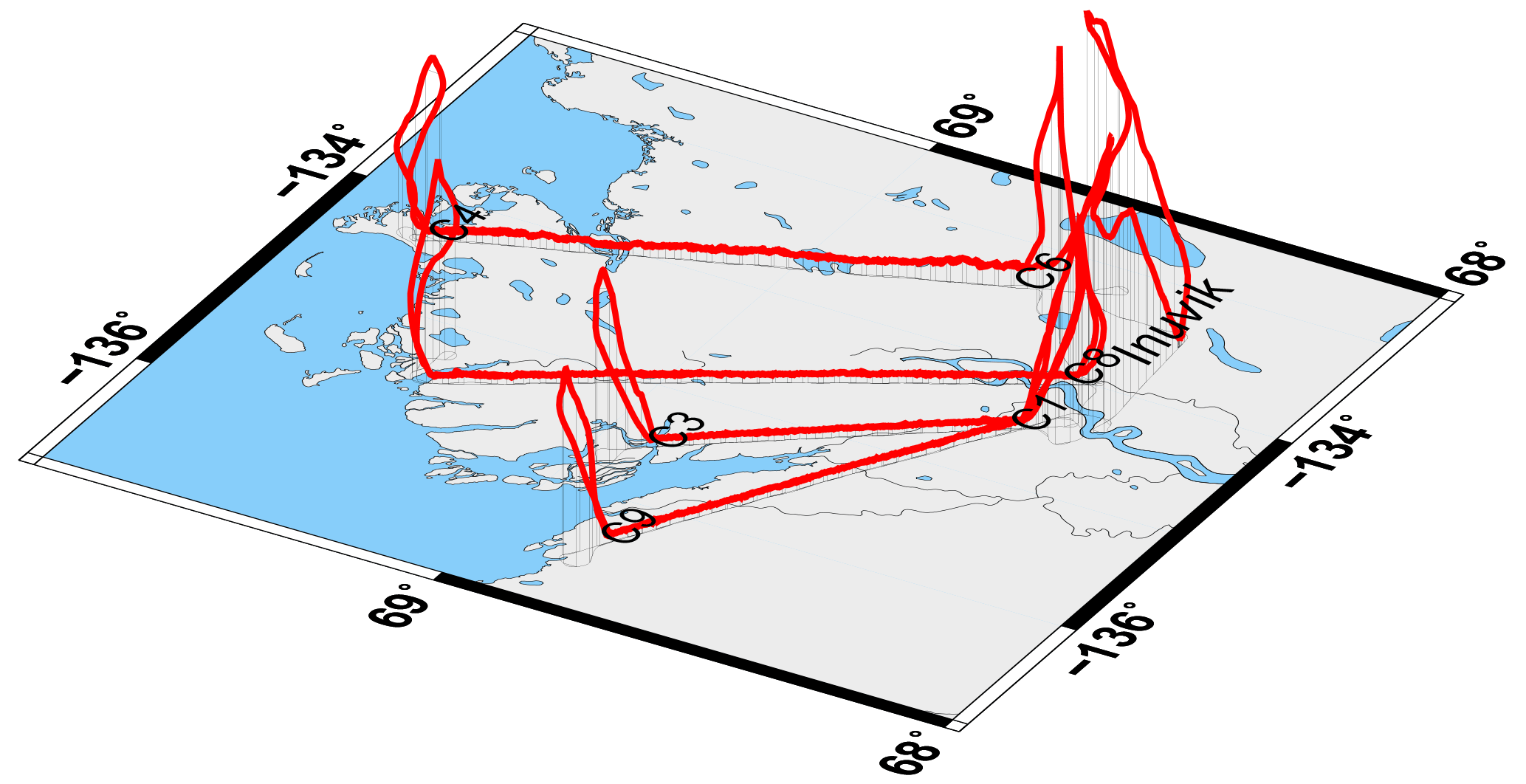
Figure 1Flight path (solid red) of Polar 5 on 20 July 2013 during the AirMeth campaign illustrating a typical pattern flown with low-level return-track flight legs and ascents and descents for profiling the convective boundary layer.
In this paper we describe the instrumentation, calibration procedures and accuracies of the wind and flux measurements. Analyses of flux patterns, footprint calculations, and correlations between fluxes and surface conditions are discussed in Kohnert et al. (2017) and Serafimovich et al. (2018).
The airborne platform we describe in this paper is the AWI (Alfred Wegener Institute) research aircraft Polar 5, a former DC 3 converted by Basler to a turboprob aircraft and now referred to as a BT-67. Polar 5 is unpressurised, is able to fly at reasonably low speed (60 m s−1 for low-level flux measurements, Ma ≈0.2) and has an endurance of 5 to 6 h.
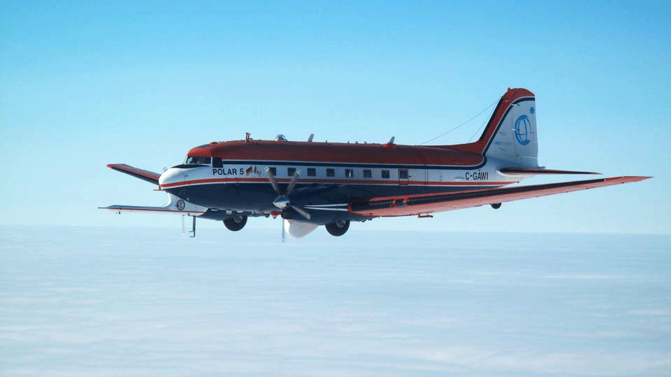
Figure 2 shows a picture of Polar 5 with the noseboom for turbulence measurements. Polar 5 is used for geosciences and atmospheric measurements and occasionally for logistics (Wesche et al., 2016). Equipment is not permanently installed, and most campaigns are flown with different instrumentation. Therefore the calibration coefficients and alignment offsets for the five-hole probe are re-examined for each reinstallation. In this paper all instrument description refer to the configuration flown in the 2012 and 2013 AirMeth campaigns.
2.1 Turbulence probe
For turbulence measurements Polar 5 can be equipped with a noseboom carrying a Rosemount 858 five-hole probe. The tip of the probe is 2.9 m ahead of the tip of the fuselage. Dynamic, static and differential pressures are measured by Rosemount pressure transducers: for the static pressure, Rosemount 1201F2A1B1B with a precision better than 0.1 hpa between 200 and 1100 hpa; for the dynamic pressure, Rosemount 1221F2VL6B1B with a precision better than 0.02 hpa for ±50 hpa; and for the flow angle differential pressures, Rosemount 1221F2VL3B1B with a precision better than 0.01 hpa for ±20 hpa. These precisions have been confirmed in laboratory calibrations with temperature variations between 0 and 20 ∘C and during ground recordings with the probe covered. The sensor head of the noseboom is manufactured by MessWERK (Cremer, 2008). The frequency response of the pressure transducers is sufficiently fast for atmospheric turbulence measurements as Lee (1993) found that for frequencies below 1 kHz any difference between source and measured signal cannot be attributed to the pressure sensors.
2.2 Position and velocity
For position, movement and attitude we use a combination of GPS and INS. The INS (inertial navigation system), a Honeywell Laseref V provides the position (longitude, latitude) at 12 Hz; the ground speed (vg), true track angle (χ) and true heading (Ψ) at 25 Hz; the pitch (Θ) and roll (Φ) angles at 50Hz; and the angular rates at 100 Hz. The accuracies for the angles, valid during all flight manoeuvres, are given as 0.1∘ for pitch and roll and 0.4∘ for true heading. The precision of the INS output data depends on the magnitude of flight manoeuvres (e.g. accelerations and turns). A comparison with a GPS-derived direction showed during a long straight and level flight. The response time of the INS is 0.02 s (as given by the manual) with a delay time of about 0.01 s. We found the time difference of 0.03 s between INS and GPS by a cross-correlation analysis of the velocity components, high-pass-filtered with a cut-off at 0.001 Hz. The position and the velocity vector are supported by Novatel GPS FlexPak6. We use the Doppler-derived velocities (“Novatel bestvel”) with a precision of 0.03 m s−1 at a data rate of 1 Hz. INS and GPS are merged by complementary filtering at a frequency of 0.1 Hz.
2.3 Temperature and humidity
High-speed temperature is recorded by an open-wire Pt100 in an unheated Rosemount housing at the tip of the noseboom with a radial distance to the centre of the five-hole probe of 16 cm and an axial distance of 35 cm. At typical measurement speed of 60 m s−1 the axial distance corresponds to a time lag of less than one sample at the recording frequency of 100 Hz. The effect of adiabatic heating due to the dynamic pressure has been taken into account. Humidity measurements are provided by a Vaisala HMT-333 mounted in a Rosemount housing in a relation to the five-hole probe similar to the fast Pt100. The HMT-333 consists of a HUMICAP and a temperature sensor in close connection. This combination allows a correction of the humidity measurement for adiabatic heating. The calibration certificate provides accuracies of ±0.4 % for the relative humidity and of C for the temperature. For cross-checks a Buck Research CR2 dew point mirror, providing highly accurate but slow absolute values, was mounted in the cabin with an inlet about 6 m aft of the five-hole probe. From 2013 on humidity was also measured in the methane analyser. Polar 5 now also has a Licor LI-7200, but it was not available in the 2012 and 2013 campaigns.
2.4 Methane analyser
In 2011 and 2012 a Los Gatos Research (LGR) Fast Methane Analyzer (FMA) was rack-mounted in the cabin. The FMA has an internal pump enabling a slow operation mode. For flux measurements the airflow through the closed cell sensor was driven by a BOC Edwards XDS35i dry scroll pump. Outside air was taken in by a rearward-facing tube 10 cm above the top of the fuselage. To achieve a high flow rate for a fast response we fed the air directly into the analyser using two filters and no air dryer. The air inlet was mounted above the cabin, 7.3 m to the rear of the tip of the five-hole probe. It was connected to the FMA by 4.3 m of stainless-steel tubing with an inner diameter of 4 mm (which is 54 mL in volume). In 2013 an LGR Fast Greenhouse Gas Analyzer (FGGA) was used instead of the FMA. All tubing remained unchanged. In addition to CH4 the FGGA also measured CO2 and H2O concentrations.
2.5 Data recorder and sampling frequencies
Polar 5 has a state-of-the-art data acquisition and management system (“DMS”) with a high-precision time based on the Precision Time Protocol according to IEEE 1588. The precision of the time stamps of all data is ±60 ns; the clock drift is less than 1 ms over 10 h. Time is synchronised to the GPS. The voltage signals of the pressure transducers of the five-hole probe and the Pt100 temperature are digitised by 16 bit AD converters and recorded at 100 Hz. The INS is recorded at the data rates mentioned above via a serial ARINC interface. Relative humidity from the Vaisala sensor and the CR2 data are recorded via a serial interface at 20 Hz and about 1 Hz, respectively. The methane data are recorded at 16 Hz in internal files by the analyser, and additionally the methane concentration is fed into the DMS via an analogue signal through the AD converters to enable synchronisation.
The wind measurement by an aircraft is the usually small difference between two larger vectors: the aircraft vector with respect to Earth Vg and the airflow vector with respect to the moving air VTAS:
Vg is given with high accuracy by the combination of INS and GPS; VTAS is based on measurements by pressure sensors at the aircraft and transformed from the aircraft system into the local Earth system by three rotations given in e.g. Lenschow and Spyers-Duran (1989) and Hartmann (1990). As modifying its surrounding pressure field is the very essence of flying an aircraft heavier than air, all pressure measurements need to be calibrated to account for these modifications. Since flying the aircraft in a wind tunnel is not an option, we have no other choice but to perform in-flight calibrations.
Calibration manoeuvres are described for single-engine aircraft e.g. by Vellinga et al. (2013) and Mallaun et al. (2015) and for twin-engine aircraft e.g. by Tjernström and Friehe (1991), Cremer (2008) and Drüe and Heinemann (2013). Typically a constant wind is assumed and speed variations are flown in box or racetrack patterns for the calibration of the dynamic pressure and in level flights for the angle of attack α. However, little attention is paid to assessing the accuracy of the assumption of a constant wind. We address that problem and describe a calibration procedure that does not need a dedicated flight pattern by exploiting a series of return-track flight legs flown for flux measurements.
3.1 True airspeed (TAS)
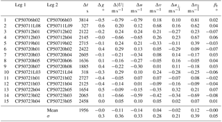
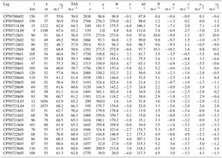
We focus on the condition of flux measurement flights, i.e. a TAS of 60 m s−1 and level flight, and use the random variations in the airspeed on manually controlled flights. For an accuracy of the wind measurement better than 0.25 m s−1 the uncertainty in the dynamic pressure needs to be smaller than 0.2 hpa. As the absolute wind is virtually never known with this accuracy, we perform reverse-heading manoeuvres during which the mean wind changes little. Furthermore we use a multitude of these manoeuvres distributed randomly in space, time and orientation over the course of the campaign. We assume that the small changes of the mean wind that might occur during individual outbound and return flights are uncorrelated between the multiple realisations of these manoeuvres. Averaging over all such pairs of flight manoeuvres will then reduce the uncertainty in the assumption of a constant wind by , with n being the number of such manoeuvres. For example with n=16, we can reduce the wind uncertainty of the calibration procedure by a factor of 4. Of all flight legs during the 2013 AirMeth campaign, 15 have been flown in reverse order in immediate succession; they are listed in Table 1 and with more details in Table A1.
For a flight track exactly parallel to a constant wind the average of the true airspeed (vT) of both legs equals the average of the true ground speed (vg) of both legs:
where the indices 1 and 2 refer to the outbound and return flight legs, respectively. For a wind deviating from the parallel to the true ground track, the aircraft heading is turned slightly into the wind, leading to a reduced ground speed. Related to this ground speed, the true airspeed is increased by 1∕cos(γ), with being the angle between the true heading Ψ and the true track χ.
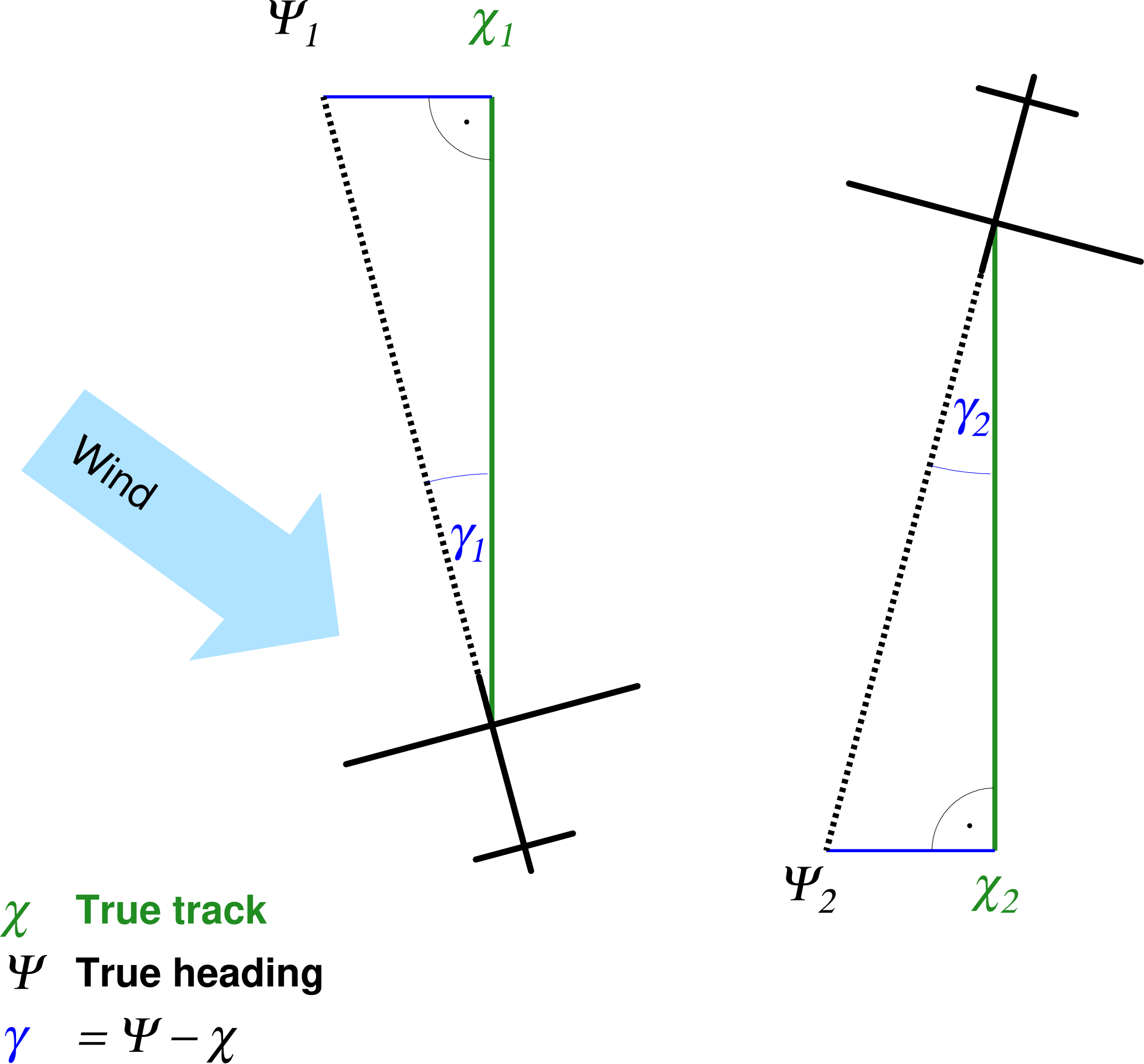
Figure 3Illustration of the angles true track χ and true heading Ψ for reverse-heading flights.
Figure 3 shows a sketch illustrating the angles. For small angles γ and with the assumptions described above, Eq. (2) becomes
with vref denoting the reference speed for this pair of return flights.
In our case is typically 2–3∘, corresponding to values for 1∕cos(γ) of ≈1.001; i.e. the reference ground speed is about 1‰ higher than the true ground speed. With vref we calculate the reference undisturbed dynamic pressure as
with ρ being the air density. Similarly we average the indicated dynamic pressure and use Eq. (4) to calibrate qi at the tip of the five-hole probe by
We find that in the range of values realised during typical low-level flux runs Eq. (5) is best approximated by a linear relationship with cq=1.165, as shown in Fig. 4.

Figure 4 Dynamic pressure derived by Eq. (4) versus the indicated dynamic pressure at the tip of the five-hole probe. Each of the 15 dots represents the average of two overpasses of the same track in reverse direction. The red line is a linear regression.
The standard deviation of the points (qc) from the approximation (1.165qi) is 0.014 hpa, which we take as an estimate of the calibration accuracy. The static pressure measurement can then be corrected by
where Δps is the measurement error of the Rosemount probe as a function of the flow angle. We use the wind tunnel measurements done by Mühlbauer (1985) with an identical Rosemount probe to approximate Δps by a second-degree polynomial:
where ϕ is the flow angle defined by cos(ϕ)=cos(α)cos(β). For flux measurement runs with α being roughly 5∘, Eq. (7) leads to a correction of typically 0.04 hpa.
Table 1Return-track flight sections used for the calibration of the dynamic pressure measurement and the alignment between the five-hole probe and the INS reference. Each line refers to one pair of return flights over the same track. The first column is sequential numbering, while the second and third columns give the codes of the flight legs; further details are listed in Table A1. Δt is the time difference between the middle of each leg, Δχ the difference in the track angle, the difference in the wind speed, Δu and Δv the differences of the horizontal wind components (u positive to the east and v positive to the north), Δu⊥ and Δv‖ the differences in components of the wind rotated to align with the track angle, and βr the remaining offset in the β angle (Eq. 12). All parameters are calculated after the calibration.
3.2 Angle of attack alpha
At the five-hole probe a pressure difference results between the two holes on the vertical plane that depends on the angle of attack α. This relation is a function of the shape of the probe and of the aerodynamical influence of the aircraft. The probe's shape has been thoroughly tested in wind tunnels (e.g. De Leo and Hagen, 1976; Mühlbauer, 1985) and analysed theoretically (Rodi and Leon, 2012) to be expressed by a linear proportionality: , with a proportionality constant of 12.67 and αi being the indicated, i.e. undisturbed, angle of attack; qα the indicated pressure difference; and qi the indicated dynamic pressure. A small dependence on the Mach number is neglected, since it is about 4 orders of magnitude smaller for the airspeed of our measurement flights. The proportionality constant is valid for a probe in an undisturbed flow, but the influence of the aircraft leads to a deviation from this number. Crawford et al. (1996) explained this deviation in terms of “lift-induced upwash” in front of the aircraft. Furthermore the α measurement needs to be aligned with the coordinate system of the INS. This alignment may be different for each reinstallation of the noseboom. Therefore an α calibration is typically done for each remounting of the probe and any change in the configuration of the aircraft. We combine the effects of probe shape and aircraft influence in a single calibration procedure. For the small angles that occur during straight level flights α depends with a very good approximation linearly on the pressure difference normalised by the dynamic pressure:
with α0 being the offset angle between the five-hole probe and the reference of the INS, and cα the proportionality constant.
3.2.1 Dedicated calibration flight
For a calibration flight pattern we use the fact that (a) with no pressure influence by the aircraft the angle of attack α equals the pitch angle during a straight and level flight with no vertical movement of the air and that (b) for a plane with fixed aerofoil (no flap movement) α varies with airspeed. This is a very commonly used method for the α calibration. We performed three low-level flight sections over water with the airspeed gradually increasing from 50 to 90 m s−1 over 5 min and decreasing back to 50 m s−1 again over 5 min. For these data Fig. 5 shows pitch versus qα∕qi. As the aircraft is manually controlled during this manoeuvre and the vertical movement of the air is not constantly zero, points scatter vertically with the vertical speed of the aircraft wg and horizontally with vertical wind velocity w. The colour coding with wg shows that most of the scatter is explained by vertical movement of the aircraft. Typically this is assumed to cancel on average (Mallaun et al., 2015), and mean values over subsections are used for the calibration. This implicitly assumes a Gaussian distribution of w and wg.
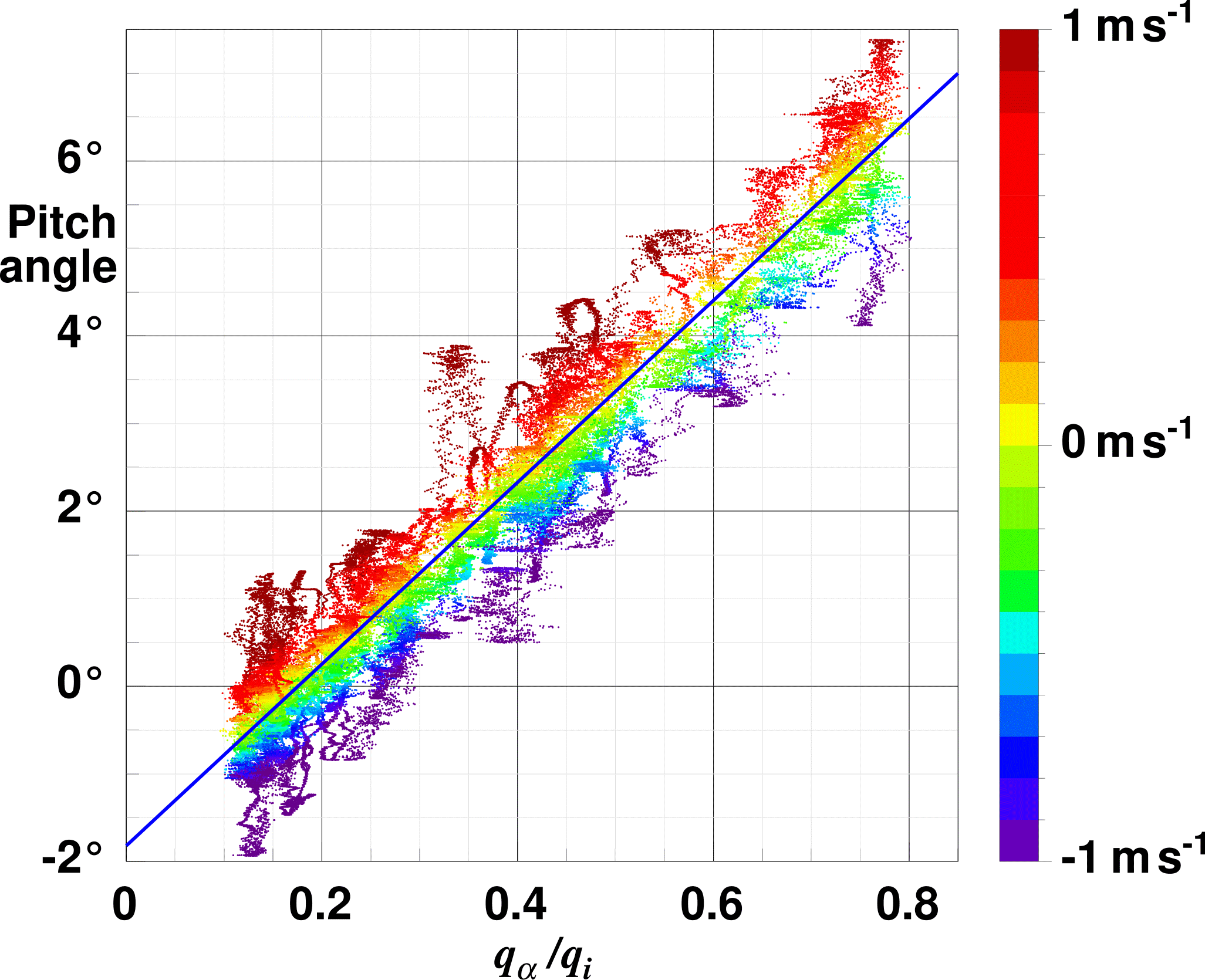
Figure 5Difference of pitch angle Θ versus alpha pressure normalised by the dynamic pressure qα∕qi. The data are from three low-level calibration flight sections over water off Barrow on 6 July 2013. Colour-coded is the vertical velocity of the aircraft wg, with the colour scale given in the vertical bar at the right. Plotted are the 100 Hz data. The blue line represents the linear regression .
With quite accurate knowledge of wg we can restrict the data used for a regression to these conditions of very little vertical movement of air and aircraft and level wings, i.e.
and furthermore correct the pitch angle by
to account for the remaining small vertical movement of the plane to arrive at
Note that for our data (Eq. 9) the correction term in Eq. (10) is smaller than 0.05∘. As the vertical wind velocity, needed for the selection condition (Eq. 9), is not known before the final calibration coefficients are determined, we need to run through one step of iteration for which we use the coefficients of the most recent campaign as a first guess. The uncertainties in the regression coefficients in Eq. (11) translate into an offset uncertainty for the vertical wind velocity of ∼0.03 m s−1 and a gain uncertainty of ∼0.7 %. Our value for cα is close to that of Mallaun et al. (2015), who found a correction factor of 0.78 necessary for a theoretical value of 12.66 to account for the aircraft influence of a Cessna Grand Caravan. A Gaussian error propagation for Eq. (8) with qi=20 hpa (TAS ≈ 60 m s−1) and qa=10 hpa (vertical wind ≈ 1 m s−1) and using the uncertainties 0.033∘ for α0, 0.073∘ for cα, 0.01 hpa for qα and 0.02 hpa for qi yield an uncertainty for α of 0.05∘, with the dominating contribution from the uncertainty of the regression slope.
3.2.2 No need for calibration flight for α
It is interesting to note that an α calibration is actually possible without any specific flight manoeuvre if sufficient data are available. We demonstrate this for the AirMeth campaign in 2013. We use all flight data of all days except 6 July 2013, the day of the dedicated α pattern, to have an independent test. Of these 68 h of flight data (with qi>10 hpa, ≅ 50 m s−1 to ensure in-flight conditions) we select those that fulfill the conditions given in Eq. (9): vertical movement of the plane smaller than 5 cm s−1, vertical wind velocity smaller than 0.1 m s−1 and roll angle smaller than 5∘ (absolute values for each). Roughly 0.6 % of the data remain and are plotted in Fig. 6 as red dots. For comparison grey shading indicates the density distribution of all 68 h of data. A least-squares fit of a linear relation results in and , which are within the range of uncertainty of Eq. (11) and differ from the values of the dedicated pattern by 1.8 % for the offset and 0.7 % for the slope. At the typical airspeed during measurement runs of 60 m s−1 the offset corresponds to constant difference for the vertical wind speed of 3 cm s−1, and the slope deviation translates directly to a gain difference of 0.7 %. Both figures are in the range of uncertainty of the results of the dedicated flight pattern.
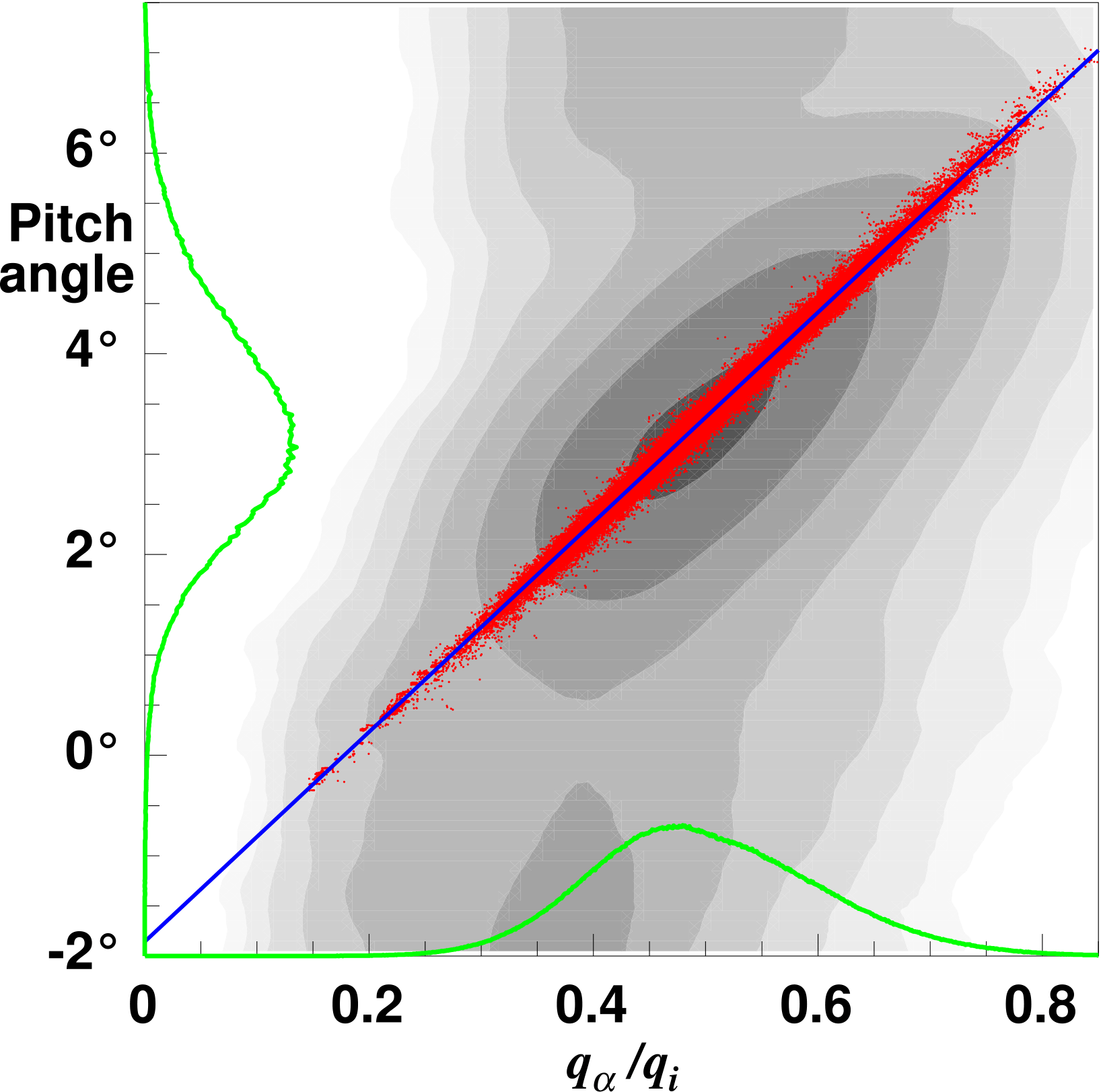
Figure 6Difference of pitch angle versus alpha pressure normalised by the dynamic pressure for all flights (except 6 July 2013) during the 2013 AirMeth campaign. Red dots are data that fulfill the conditions given in Eq. (9) and with correction of the pitch angle (Eq. 10). Grey shading indicates the distribution of all data which include ascents, descents, and take-off and landing procedures. A logarithmic shading scale is used. Only data with qi<10 hpa (corresponding to TAS =50 m s−1) are excluded to ensure in-flight conditions. The green lines show the normalised frequency distribution of all data of the horizontal level runs used for flux measurements. The blue line represents the regression .
From Fig. 6 we can furthermore see that the pitch variation during measurement runs is nearly Gaussian-distributed, while the pressure ratio qα∕qi is positively skewed due to the skewness of w at low level in a convective boundary layer (Hunt et al., 1988).
3.3 Alignment of the five-hole probe and INS reference (beta offset)
The angle of sideslip β is measured by the five-hole probe via the pressure difference qβ between the two holes on the horizontal plane. Then β is calculated by
where β0 is the alignment offset between the five-hole probe and the INS reference system, and cβ in analogy to cα (Eq. 8) is a proportionality constant. For a symmetrical sonde in a pressure field undisturbed by the aircraft cα and cβ would be identical, as e.g. Mühlbauer (1985) proved in a wind tunnel. But as we include in the calibration the influence of the aircraft pressure field which is not symmetrical with respect to the longitudinal axis of the sonde, cα and cβ are different. The proportionality cβ should not change between campaigns, but β0 needs to be recalibrated with each remounting of the noseboom. We use cβ=11.36 as determined in the calibration flights of Cremer (2008) and confirmed by Drüe and Heinemann (2013). Based on the assumption that the wind is constant for the outbound and return flights, the wind components orthogonal to the track (, after the coordinate system has been rotated to align with the track direction) should cancel out. Note that the coordinate system of the return flight is rotated by 180∘ and thus this component changes sign. A misalignment of the five-hole probe with the INS would then result in a residual of the sum of . This residual can be referenced to the misalignment by
as a residual offset for the beta angle. With the large number of return-track flights under different situations and on different days we can assume that possible wind changes are randomly distributed. Thus, the wind-induced part of βr should also be randomly distributed and cancel out when averaged over a sufficiently large number. We then manually iterate the beta offset β0 such that the average over all βrs is minimised. For the AirMeth 2013 flights we find . Mallaun et al. (2015) pointed out that a misalignment of the β angle should show in a correlation between the vertical wind velocity and the roll angle, as a misaligned sonde would be tilted up- or downward and thus produce a spurious vertical wind. Following their suggestion, we tested for the alignment-corrected wind calculation for and m s−1 and could not find any correlation.
3.4 Static pressure precision
We can use the series of return-track flights for an estimation of the precision of the static pressure measurement. As we have passed the same location during the return flight (with about ±200 m lateral deviation), we can calculate a pressure difference along the track. This difference is composed of sensor uncertainties, height variation of the aircraft and atmospheric change. The height variation is accounted for by calculating the static pressure for a reference height href by
with ps being the static pressure (Eq. 6), g the acceleration due to gravity, R the gas constant for air and T the temperature. As a reference height we define the mean over both flight legs. The atmospheric change is handled by this procedure: for each position along the track we have a
the absolute value of the pressure difference between both passes, and in analogy a Δt, the time elapsed between both overpasses. Plotting Δp versus Δt shows increasing scatter with increasing Δt. A least-squares fit gives with its ordinate offset at Δt=0 the remaining uncertainties of the sensors. We find this Δp0 to be <0.1 hpa. This uncertainty estimate includes the uncertainty of the direct pressure measurement as well as that due to the aircraft height based on the GPS data. With this uncertainty a pressure gradient detection limit for a 100 km long leg would be 0.001 hpa km−1. Note that this method can only estimate the relative accuracy; a constant offset in the static pressure measurement cannot be detected.
3.5 Accuracy of the horizontal wind measurement
The difference in the mean wind speed between outbound and return legs as shown in Table 1 has a mean value of 0.08 m s−1 and a standard deviation of 0.33 m s−1 over all 15 pairs. This supports our assumption that mostly results from atmospheric variation and that the calibration and measurement uncertainty rather is of the order of 0.08 m s−1. Rotating the wind components into an along-track component v‖ and an across-track component u⊥, we get a mean difference in v‖ of 0.11 m s−1, which translates into a calibration uncertainty for the dynamic pressure of ≈0.09 hpa and is of similar order to the estimate given in Sect. 3.1. Calculating a Gaussian error propagation for the along-track component
using the uncertainties 0.1 hpa for the static pressure p, 0.12 hpa (averaging the estimates of Sect. 3.1 and 3.5) for the dynamic pressure qi, 0.1 K for the temperature T and 0.03 m s−1 for the ground speed vg‖ results in an uncertainty for v‖ of 0.18 m s−1. In this estimate the uncertainty of qi clearly dominates the other contributions by about 1 order of magnitude. Note that this estimate is valid for wind measurements during horizontal flight legs. The accuracy during turn manoeuvres, ascents and descents may be less. For the alignment offset between the five-hole probe and the INS we estimate the calibration uncertainty by the standard deviation of βr, given in Table 1 (second-to-last line) to be 0.05∘. Furthermore, applying the procedure described in Sect. 3.4 to the horizontal wind components yields 0.2 m s−1 as an uncertainty estimate for both components, confirming the estimate in this section.
3.6 Methane analyser
The data acquisition system of Polar 5, DMS, and the methane analyser each ran on an autonomous computer system with its individual clocks. They were synchronised by recording within the DMS an analogue output of the methane analyser. Sectionwise cross correlation revealed that the analyser's clock ran typically slower than the DMS. This synchronisation was done individually for each flight leading to a timing accuracy of 0.01s between the systems.
After clock synchronisations, the time lag of the methane signal due to delay in the tubings was found by a cross-correlation analysis of the FGGA data with the vertical wind velocity for selected runs with clearly positive methane and humidity fluxes. Prior to the correlation analysis all signals were high-pass-filtered with a cut-off at 0.1 Hz (corresponding to ≈600 m horizontal distance at 60 m s−1). The time lags for CH4, CO2 and H2O are 0.68, 0.66 and 0.72 s, respectively, with negligible variation between individual runs. Water vapour has a slightly larger delay due to interaction with the tubing. However, as Ibrom et al. (2007) have shown, for referencing the methane signal to a dry mole fraction the water vapour signal needs to be treated with the same time delay as the methane signal, as the actual condition in the measurement cell is relevant. A correlation analysis between the FGGA and Vaisala humidity signals showed a delay of 0.36 s of the Vaisala signal. The time delay of the methane signal due to the tubing was confirmed by a ground test. A step change of the concentration at the inlet took 0.5 s to arrive at the analyser's reading.
The cell pressure in the methane analyser is maintained at 140 Torr and shows little variation during level flux measurement runs. Desjardins et al. (2017) used a Picarro G2301-f in a Twin Otter for flux measurements and found a weak correlation of the methane concentration with the cell pressure. We performed coherency and correlation analysis with spectral resolution and as integral statistics and could not find any correlation between pressure and the CH4 signal. Also Wolfe et al. (2018) reported no pressure effect on the CH4 signal from an airborne LGR analyser.
A specific problem of airborne cavity ring-down spectroscopy, especially in the Arctic, is sensor warm-up. In a flux tower setup sensors typically run continuously, but for airborne applications the instruments can only be switched on after starting of the engines. Occasionally sensors could be pre-heated by ground power, but this was not always available. Laboratory and in-flight tests showed that the CH4 concentration reported from a cold sensor increased with cavity temperature for temperatures lower than 34 ∘C. For below-zero starting conditions, warm-up time was up to 45 min.
To analyse the accuracy of airborne trace gas flux measurements, we estimate the flux detection limit, test the instrument precision and use a spectral analysis to compare methane fluxes with the well-known behaviour of heat and moisture fluxes. We focus on the covariance at the height of the aircraft. For referencing the flux measurement to the surface level and footprint calculations we refer to Kohnert et al. (2017) and Serafimovich et al. (2018).
4.1 Instrumental noise
To determine the instrumental noise level from our recordings, we follow a method described by Mauder et al. (2013), based on the property of univariate white noise being uncorrelated with the signal. Thus it appears only at lag 0 of the autocorrelation but not in further lags. The variance of the noise error ϵx2 of a quantity x can be estimated as
where C11(0) is the autocorrelation of x at lag 0 and C11(p→0) the autocorrelation as a function of lag p extrapolated to lag 0. For the FGGA we get ϵx=0.0037 ppm for CH4, ϵx=0.695 ppm for CO2 and ϵx=34.9 ppm for H2O, all confirming the design specifications of the instrument. Applying the same procedure to the data of vertical wind velocity and temperature, we get ϵx=0.029 m s−1 for w and x=0.0022 K for Tϵ. For C11(p→0) we use the lags 3–20, corresponding to 0.16 to 1.0 s sampling time.
4.2 Turbulent flux detection limit
Next we determine the turbulent flux detection limit, now based on the property of the bivariate white noise being uncorrelated with the signal.
First, we use a method suggested by Wienhold et al. (1995) based on the cross-covariance function. Here, the correlation between biophysical (scalar abundance) and transport (air motion) mechanisms is removed by shifting the two time series against each other, leaving only the random correlations attributed to instrumental noise. We calculate the standard derivation of the cross-covariance function for the time lag interval −200 to −50 and 50 to 200 s. At a typical airspeed of 60 m s−1 this corresponds to shifting the two time series by 3 to 12km horizontal distance.
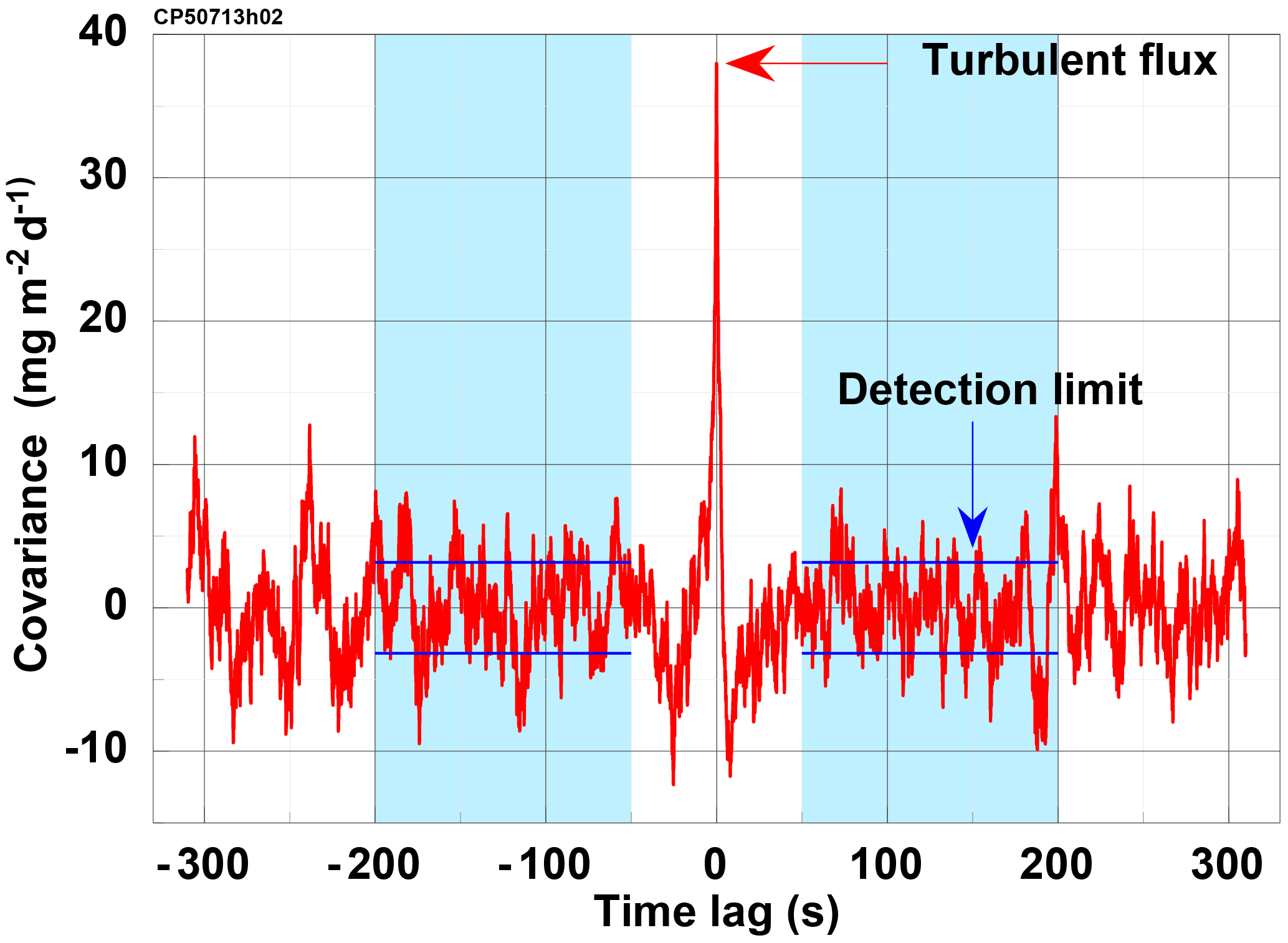
Figure 7Example of the covariance function of w′ and versus time lag to illustrate the range used for estimation of the flux detection limit. The covariance is scaled to mg m2 d−1. Blue shaded areas indicate the ranges −200 to −50 and 50 to 200 s, over which the standard deviation has been calculated; it is marked by the horizontal blue lines. At the typical airspeed of 60 m s−1 the range corresponds to 3 to 12 km. The figure shows data of run CP50713h02 with a methane flux of 30.9 mg m2 d−1 (at lag zero, marked by the red arrow). The standard derivation over the range marked blue is 3.1 mg m2 d−1, which is taken as an estimate for the flux detection limit.
Figure 7 shows an example of a horizontal flight section on 13 July 2013, where the turbulent flux is marked at lag 0 and the estimate for the detection limit is as described above by blue lines.
Applying this procedure to all horizontal flight legs of the 2013 campaign with positive methane, heat and moisture fluxes and negative CO2 fluxes and averaging, we get detection limits of 3.9 mg m−2 d−1 for , 1.4 g m−2 d−1 for , 4.2 W m−2 for the sensible heat flux and 8.8 W m−2 for the latent heat flux.
Billesbach (2011) provides an alternative “random shuffle” method for determining the turbulent flux detection limit: here the bivariate white noise property is achieved by recalculating the eddy covariance after one of the variables has been randomly “time-shuffled” instead of shifted. When applied to all 44 low-level flight legs of the AirMeth 2012 North Slope campaign, this method yields comparable flux detection limits of 4.9±1.4 g m2 d−1, 4.6±1.9 W m2 and 3.9±1.3 W m2 for the fluxes of methane, sensible and latent heat, respectively. The LGR FMA sensor installed in 2012 did not measure CO2.
4.3 Spectral analysis
With the precision of ±3 ppb for an integration time of 0.1 s of the methane analyser we cannot expect to have spectral resolution of atmospheric fluctuations in the high-frequency (HF) range that is comparable to temperature and vertical velocity. We examine power spectra (Fig. 8) of a 100 km long flight leg at 50 m above ground. The measurements were taken on 12 July 2013 over the North Slope of Alaska in a convective boundary layer driven by a sensible heat flux of 70 W m−2. The boundary layer height zi was 500 m.
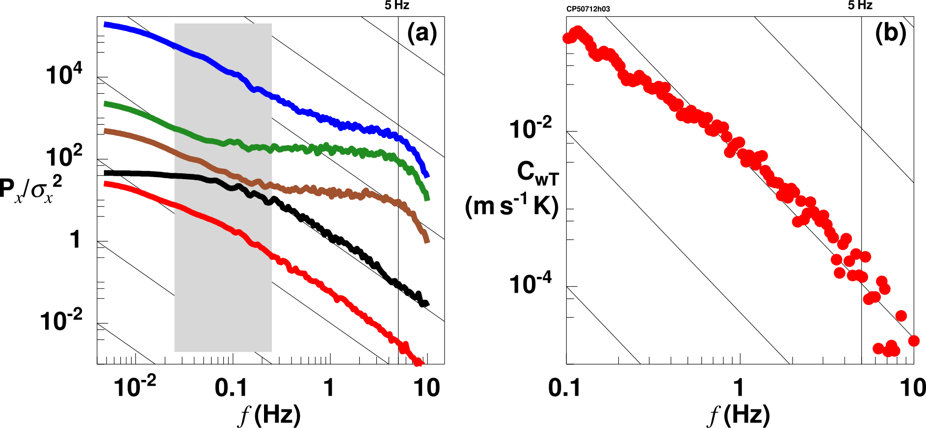
Figure 8(a) Power spectra of the fluctuation of temperature (red), vertical wind velocity (black), CH4 (brown), CO2 (green) and water vapour mixing ratio (blue). The spectra are nondimensionalised by their respective variance and shifted in the plot by 1 decade increasingly. The sloped lines indicate a decrease. The grey shaded area marks the scale corresponding to 5–0.5 zi, the range of dominant transport in a convective boundary layer. (b) Covariance spectrum of vertical wind velocity and temperature. The sloped lines indicate decrease. Data are from 12 July 2013 at the Alaskan North Slope, with measurement height of 50 m above ground and boundary layer height zi=500 m above ground.
Vertical wind velocity and temperature nicely follow a drop-off over nearly 2 decades for horizontal scales smaller than the boundary layer height. The data from the FGGA contain considerable white noise, most pronounced for CO2, followed by CH4, and least for the water vapour measurement. All three show too much HF noise to resolve the inertial subrange of turbulence. Similar results are shown by Wolfe et al. (2018) from low-level airborne carbon flux measurements over Maryland and Virginia. Beyond about 5 Hz (corresponding to 12 m horizontal distance at the typical airspeed of 60 m s−1) spectral drop-off due to dampening in the tubing is visible. As w scales with the boundary layer height, power at the low-frequency end does not increase further, while the fluctuations in all scalars continue on scales far beyond 100× the boundary layer height since the scalar quantities rather scale with their horizontal surface structure.
In the cospectrum of w and T we see the expected drop-off (e.g. Kaimal et al., 1972), as shown in Fig. 8. Beyond 5 Hz there appears a small drop-off; however, theses scales (corresponding to 12 m horizontal resolution) contribute a negligible amount to the covariance at the aircraft height of 50 m. The uncertainties at the low-frequency end are larger and more important for flux estimates.
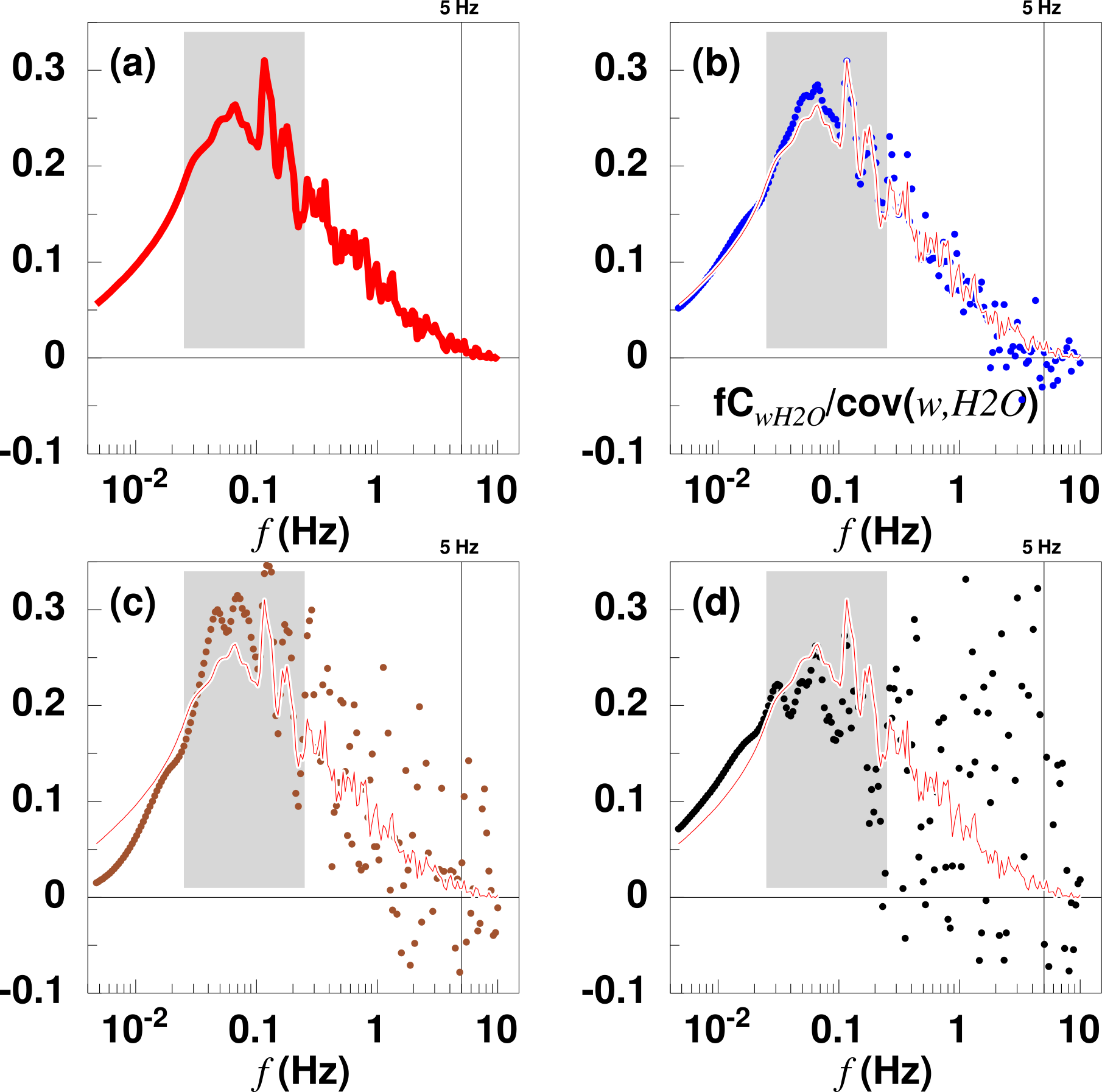
Figure 9Cospectra normalised by their respective covariances. The data are from the same flight leg as in Fig. 8. The grey shaded areas mark the scales corresponding to 5–0.5 zi. (a) CwT sensible heat flux, red; (b) C moisture flux, blue; (c) C methane flux, brown; and (d) C flux of carbon dioxide, black. Note that normalisation by the covariance eliminates the sign. The first three fluxes are directed upward; the carbon dioxide flux is downward. For comparison CwT is plotted as thin red line in (b), (c) and (d).
Since the white noise of the trace gas analyser is uncorrelated with the vertical velocity, it does not appear in the covariance spectra (Fig. 9). All four spectra are of similar shape. Although C and C have considerably more scatter in the high frequencies, their drop-off follows that of CwT. Thus the turbulent vertical transport of trace gases is essentially identical to that of other scalars in the convective boundary layer.
Uncorrelated instrumental noise should vanish, or at least reduce, if measurements are repeated under similar conditions and averaged. The statistical error then reduces proportionally to , with n being the number of independent realisations. We calculated covariance spectra for each of the 93 available low-level legs of the 2013 AirMeth campaign, normalised by their covariance and averaged. In these stacked cospectra (Fig. 10) the expected drop-off is reproduced for all four scalar fluxes, again, with more scatter for the trace gases than for the water vapour or the temperature. Figure 10 shows that the instrumental noise leading to the spectral deviation in Fig. 8 is uncorrelated with the vertical velocity and does not affect the covariance other than by a small increase of statistical uncertainty.
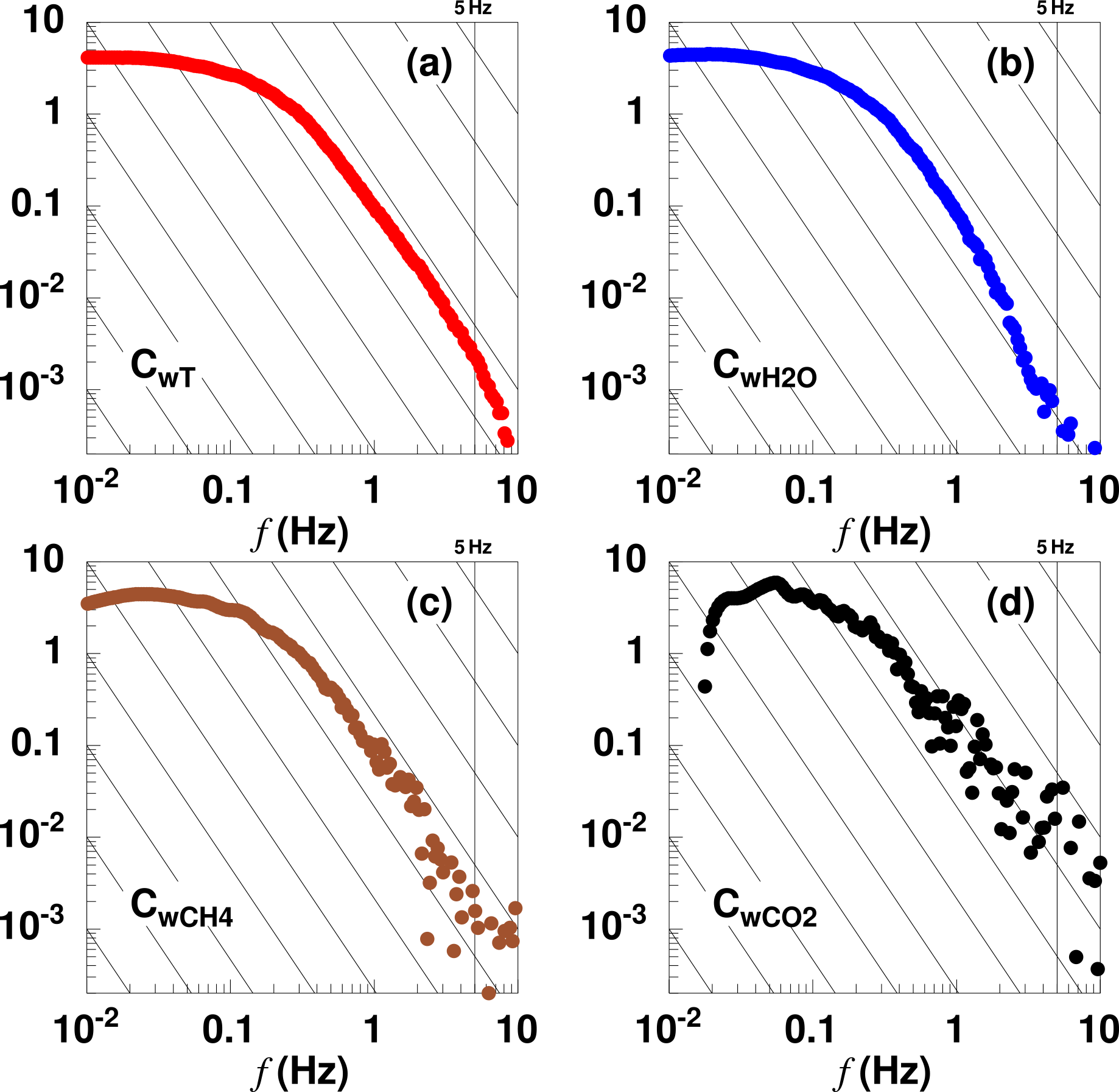
Figure 10Stacked cospectra normalised by their respective covariances. The spectra are averages of 87 horizontal flight legs totalling some 5600 km distance and 26 h. (a) CwT sensible heat flux, red; (b) C moisture flux, blue; (c) C methane flux, brown; and (d) C flux of carbon dioxide, black. Note that normalisation by the covariance eliminates the sign. Thin black lines show the slope.
4.4 Dry mole fraction flux
We aim to determine the mass of methane being emitted from the surface per area unit and time interval. The trace gas analyser measures molecular ratios. As the atmospheric methane concentration is of a similar order of magnitude to the density variations due to humidity fluctuations, the latter need to be taken into account in computing a mass flux from the measured (wet) mole fractions (Webb et al., 1980).
A direct measurement of dry mole fractions requires gas drying. However, for eddy covariance analysis a fast response of the system is very important. To keep the tubing as short as possible, we fed the outside air directly into the analyser, avoiding delays by an air dryer, and account for the effect of humidity fluctuations by using fast humidity measurements. This method can even be applied in the tropics with considerably higher atmospheric humidity as Chen et al. (2010) have proven. To then find the dry mole fraction flux, two options remain:
-
Finding for each CH4 sample taken in the measurement cell the exact humidity in the very same moment. For this method either an additional humidity measurement needs to be done in the analyser cell, or a separate fast humidity measurement can be referenced into the analyser with a high temporal accuracy.
-
Calculating a wet mole fraction flux and applying what is commonly referred to as one of two Webb–Pearman–Leuning (WPL) correction terms (Webb et al., 1980). For method (2) a separate humidity flux measurement needs to be available.
With the FGGA used in the 2013 AirMeth campaign the water vapour concentration is measured in the same air volume and at the same time as the trace gas concentration. Dry mole fraction can then be calculated by
where is the ratio of water vapour to dry air. The dry mole flux then is
with being the density of methane. We use these data to estimate differences and possible inaccuracies introduced by the above-mentioned methods. We compare the dry mole fraction flux based on CH4 with the following four different methods:
- a.
Based on CH4w plus the WPL term calculated from the FGGA-humidity measurement.
ma∕mv is the mass ratio of dry air and water vapour; ρCH4 and ρa are the densities of methane and dry air, respectively; and ρvFGGA is the water vapour density as measured by the FGGA. F and FA should only be affected by numerical inaccuracies. The ratio FA∕F turns out to be 0.993±0.002.
- b.
Based on CH4w plus the WPL term taken from the Vaisala humidity measurement.
The ratio FB∕F turns out to be 1.041±0.035. The overestimation of 4.1 % is due to the fact that the Vaisala measurement leads to a 31.2 % larger humidity flux than the FGGA measurement. However a direct comparison between averaged humidity measurements shows a good agreement. The flux difference is due to a different response behaviour of both sensors. Since in the 2012 campaign no other fast humidity measurement was available, this method had to be applied, leading to a slightly increased uncertainty of the methane flux. Assuming a similar behaviour for 2012 to that for 2013, we overestimate the methane fluxes by roughly 4 %.
- c.
Based on CH4dvais as calculated from CH4w and the in-cell humidity derived from the (outside) Vaisala measurement (HMT-330) referenced into the analyser cell. We calculated the mixing ratio from the relative humidity, temperature (Pt100) and pressure and determined the time lag to the humidity measurement of the FGGA by a cross correlation of the high-pass-filtered data to be 1.12 s and time-shifted the data by this amount. Thus
and the flux
The ratio FC∕F turns out to be 1.080±0.047, somewhat larger than method (b) mostly due to the apparently insufficiently accurate time shift procedure. However, this method had to be used for the 2012 data (e.g. Kohnert et al., 2017) to enable wavelet decomposition.
- d.
No correction for water vapour.
The ratio FD∕F is 0.793±0.093. Thus, for our situation of methane emissions from Arctic tundra the water vapour fluctuations lead to a flux underestimation of 20 % if not accounted for.

Figure 11 Comparison of different methods of accounting for humidity fluctuations in estimating methane flux from wet mole fraction measurements. The abscissa is the dry mole flux, F (Eq. 18). Dark yellow is FB, the wet mole flux plus WPL term based on the Vaisala data according to Eq. (20). Green represents FC (Eq. 21), and medium blue is the uncorrected wet mole flux, FD (Eq. 22).
Figure 11 shows the above for each horizontal flight section of the 2013 AirMeth campaign. We conclude that, even with a non-perfect humidity flux measurement, the dry mole fraction flux can be determined in polar regions with reasonable accuracy, in our case of the 2012 campaign an over-estimation of 4 %.
We showed that aircraft are well-suited tools for studying methane emissions from Arctic tundra. The vertical fluxes of the most important greenhouse gases can be measured during low-level flight legs with sufficient accuracy. We showed that a calibration of the essential coefficients of aircraft turbulence equipment can be achieved with high accuracy by exploiting suitably arranged flux measurement legs. The natural variations in parameters (airspeed, pitch) due to manually controlled flights are sufficient. The horizontal wind components are measured with an accuracy better than 0.2 m s−1 during level flight legs. The level of white noise of the trace gas analyser does not allow the inertial subrange of turbulent fluctuations of CO2 and CH4 to be resolved with sufficient accuracy. However, since the noise is uncorrelated with the vertical wind velocity, the cospectra show a drop-off if sufficient data are available for averaging. We found the detection limit of the methane flux to be about 4 mg m−2 d−1 and that of carbon dioxide to be about 1.4 g m−2 d−1.
The data are available on request from the lead author.
A list of these pairs of flight legs is given in Table A1.
Table A1Horizontal flight legs used for the calibration of the dynamic pressure measurement and the alignment between the five-hole probe and the INS reference. The first column gives the code of the flight leg; further details and a full list of all flight legs of the AirMeth campaign 2013 are given in Kohnert et al. (2014). l is the leg length; h is the height above ground; vg is the averaged ground speed; TAS is the averaged true air speed; t is the time needed to fly the legs; χ is the true track angle; Ψ is the true heading; is the angle between heading and track; dd and ff are the wind direction and speed, respectively; u and v are the wind components (u positive to the east and v positive to the north); and u⊥ and v‖ are the components of the wind rotated to align with the track angle. All parameters are calculated after the calibration.
JH devised the calibration procedures and wrote the manuscript with contributions from co-authors. MG designed the installation of the instrumentation. JH and TS designed the campaign and collected the data together with KK and MG. KK performed additional calibrations of the methane analyser. SM calculated the instrumental noise and described the detection limit.
The authors declare that they have no conflict of interest.
We thank the pilots, mechanics and engineers for their support. We thank Matthias Cremer for fruitful discussions and two anonymous reviewers for helpful comments.
The AirMeth campaigns were fully funded by Alfred
Wegener Institute Helmholtz Centre for Polar and Marine Research. This work has
received funding from the Helmholtz Association of German Research Centres through a
Helmholtz Young Investigators Group grant to Torsten Sachs (grant VH-NG-821) and is a
contribution to the European Union's Horizon 2020 research and innovation programme
under grant agreement no. 727890, as well as to the Helmholtz Climate Initiative
(REKLIM – Regional Climate Change). The National Ecological Observatory Network is a
project sponsored by the National Science Foundation and managed under cooperative
agreement by Battelle Ecology, Inc. This material is based upon work supported by the
National Science Foundation (grant DBI-0752017). Any opinions, findings, and
conclusions or recommendations expressed in this material are those of the authors and
do not necessarily reflect the views of the National Science Foundation.
The article processing charges for this open-access
publication were covered by a
Research
Centre of the Helmholtz Association.
Edited by: Christian Brümmer
Reviewed by: two anonymous referees
Baer, D. S., Paul, J. B., Gupta, M. and O'Keefe, A.: Sensitivity absorption measurements in a near-infrared region using off-axis integrated-cavity-output spectroscopy, Appl. Phys. B, 75, 261–265, https://doi.org/10.1007/s00340-002-0971-z, 2002. a
Billesbach, D. P.: Estimating uncertainties in individual eddy covariance flux measurements: A comparison of methods and a proposed new method, Agr. Forest Meteorol. 151, 394–405, https://doi.org/10.1016/j.agrformet.2010.12.001, 2011. a
Bousquet, P., Ringeval, B., Pison, I., Dlugokencky, E. J., Brunke, E.-G., Carouge, C., Chevallier, F., Fortems-Cheiney, A., Frankenberg, C., Hauglustaine, D. A., Krummel, P. B., Langenfelds, R. L., Ramonet, M., Schmidt, M., Steele, L. P., Szopa, S., Yver, C., Viovy, N., and Ciais, P.: Source attribution of the changes in atmospheric methane for 2006–2008, Atmos. Chem. Phys., 11, 3689–3700, https://doi.org/10.5194/acp-11-3689-2011, 2011. a
Cambaliza, M. O. L., Shepson, P. B., Caulton, D. R., Stirm, B., Samarov, D., Gurney, K. R., Turnbull, J., Davis, K. J., Possolo, A., Karion, A., Sweeney, C., Moser, B., Hendricks, A., Lauvaux, T., Mays, K., Whetstone, J., Huang, J., Razlivanov, I., Miles, N. L., and Richardson, S. J.: Assessment of uncertainties of an aircraft-based mass balance approach for quantifying urban greenhouse gas emissions, Atmos. Chem. Phys., 14, 9029–9050, https://doi.org/10.5194/acp-14-9029-2014, 2014. a
Chen, H., Winderlich, J., Gerbig, C., Hoefer, A., Rella, C. W., Crosson, E. R., Van Pelt, A. D., Steinbach, J., Kolle, O., Beck, V., Daube, B. C., Gottlieb, E. W., Chow, V. Y., Santoni, G. W., and Wofsy, S. C.: High-accuracy continuous airborne measurements of greenhouse gases (CO2 and CH4) using the cavity ring-down spectroscopy (CRDS) technique, Atmos. Meas. Tech., 3, 375–386, https://doi.org/10.5194/amt-3-375-2010, 2010. a
Crawford, T. L., Dobosy, R. J. and Dumas, E .J.: Aircraft wind measurement considering lift-induced upwash, Bound.-Lay. Meteorol., 80, 79–94, 1996. a
Cremer, M.: Kalibrierung der Turbulenzmessonde der Polar 5, Dok.-Nr.mW-AWI-P5-2008-06, Messwerk, Braunschweig, Germany, 2008. a, b, c
De Leo, R. V. and Hagen, F. W.: Aerodynamic performance of Rosemount model 858AJ air data sensor, Rosemount Report 8767, Aeronautical Research Department, Rosemount Inc., P.O. Box 35129, Minneapolis, Minnesota 55435 USA, 1976. a
Desjardins, R. L., Wortha D. E., Pattey, E., VanderZaaga, A., Srinivasan, R., Mauder, M., Worthy, D., Sweeney, C., and Metzger, S.: The challenge of reconciling bottom-up agricultural methane emissions inventories with top-down measurements, Agr. Forest Meteorol. 248, 48–59, https://doi.org/10.1016/j.agrformet.2017.09.003, 2017. a, b
Dobosy, R., Sayres, D., Healy, C., Dumas, E., Heuer, M., Kochendorfer, J., Baker, B., and Anderson, J.: Estimating Random Uncertainty in Airborne Flux Measurements over Alaskan Turdra: Update on the Flux Fragment Method, J. Atmos. Ocean. Tech., 34, 1807–1822, 2017. a
Drüe, C. and Heinemann, G.: A Review and Practical Guide to In-Flight Calibration for Aircraft Turbulence Sensors, J. Atmos. Oceanic Technol., 30, 2820–2837, https://doi.org/10.1175/JTECH-D-12-00103.1, 2013. a, b
Hartmann, J.: Airborne Turbulence Measurements in the Maritime Convective Boundary Layer, PhD Thesis, Flinders University of South Australia, 163 pp., 1990. a
Hiller, R.V., Neininger, B., Brunner, D., Gerbig, C. Bretscher, D., Künzler, T., Buchmann, N., and Eugster, W., Aircraft-based CH4 flux estimates for validation of emissions from an agriculturally dominated area in Switzerland, J. Geophys. Res.-Atmos., 119, 4874–4887, 2014. a
Hunt, J. C. R., Kaimal, J. C., and Gaynor, J. E.: Eddy structure in the convective boundary layer – new measurements and new concepts, Q. J. Roy. Meteor. Soc., 144, 827–858, 1988. a
Ibrom, A., Dellwik, E., Larsen, S. E., and Pilegaard, K.: On the use of the Webb–Pearman–Leuning theory for closed-path eddy correlation measurements, Tellus, 59B, 937–946, 2007. a
Kaimal, J. C., Wyngaard, J. C., Yzumi, Y., and Coté, O. R.: Spectral characteristics of surface-layer turbulence, Q. J. Roy. Meteor. Soc. 98, 563–589, 1972. a
Karion, A., Sweeney, C., Pétron, G., Frost, G., Hardesty, R. M., Kofler, J., Miller, B. R., Newberger, T., Wolter, S., Banta, R., Brewer, A., Dlugokencky, E., Lang, P., Montzka, S. A., Schnell, R., Tans, P., Trainer, M., Zamora, R., and Conley, S.: Methane emissions estimates from airborne measurements over a western United States natural gas field, Geophys. Res. Lett., 40, 1–5, https://doi.org/10.1002/grl.50811, 2013. a
Kohnert, K., Serafimovich, A., Hartmann, J. ,and Sachs, T.: Airborne Measurements of methane fluxes in Alaskan and Canadian Tundra with the Research Aircraft Polar 5, Reports on Polar and Marine Research, 673, 2014. a
Kohnert, K., Serafimovich, A., Metzger, S., Hartmann, J., and Sachs, T.: Strong geologic methane emissions from discontinuous terrestrial permafrost in the Mackenzie Delta, Canada, Scientific Reports, 7, 5828, 2017. a, b, c, d
Lee, M. F.: Dynamic response of pressure measuring systems, Technical Report 32, Department of Defence, Defence Science and Technology Organisation, Aeronautical Research Laboratory, Melbourne, Vic. Australia, April 1993. a
Lenschow, D. H. and Spyers-Duran, P.: Measurement techniques: Air motion sensing, NCAR Research Aviation Facility Bull. 23, 36 pp., available from: NCAR, P.O. Box 3000, Boulder, CO 80307., 1989. a
Mallaun, C., Giez, A., and Baumann, R.: Calibration of 3-D wind measurements on a single-engine research aircraft, Atmos. Meas. Tech., 8, 3177–3196, https://doi.org/10.5194/amt-8-3177-2015, 2015. a, b, c, d
Mauder, M., Desjardins, R. L., and MacPherson, I.: Creating surface flux maps from airborne measurements: Application to the Mackenzie area GEWEX study MAGS 1999, Bound. Lay. Meteorol., 129, 431–450, https://doi.org/10.1007/s10546-008-9326-6, 2008. a
Mauder, M., Cuntz M., Drüe, C., Graf, A., Rebmann, C., Schmid, H.P., Schmidt, M., and Steinbrecher, R.: A strategy for quality and uncertainty assessment of long-term eddy-covariance measurements, Agr. Forest Meteorol. 169, 122–135, https://doi.org/10.1016/j.agrformet.2012.09.006, 2013. a
McGuire, A. D., Christensen, T. R., Hayes, D., Heroult, A., Euskirchen, E., Kimball, J. S., Koven, C., Lafleur, P., Miller, P. A., Oechel, W., Peylin, P., Williams, M., and Yi, Y.: An assessment of the carbon balance of Arctic tundra: comparisons among observations, process models, and atmospheric inversions, Biogeosciences, 9, 3185–3204, https://doi.org/10.5194/bg-9-3185-2012, 2012. a
Metzger, S., Junkermann, W., Mauder, M., Butterbach-Bahl, K., Trancón y Widemann, B., Neidl, F., Schäfer, K., Wieneke, S., Zheng, X. H., Schmid, H. P., and Foken, T.: Spatially explicit regionalization of airborne flux measurements using environmental response functions, Biogeosciences, 10, 2193–2217, https://doi.org/10.5194/bg-10-2193-2013, 2013. a
Miller, S. M., Miller, C. E., Commane, R., Chang, R. Y.-W., Dinardo, S. J., Henderson, J. M., Karion, A., Lindaas, J., Melton, J. R., Miller, J. B., Sweeney, C., Wofsy, S. C., and Michalk, A. M.: A multiyear estimate of methane fluxes in Alaska from CARVE atmospheric observations, Global Biogeochem. Cy., 30, 1441–1453, https://doi.org/10.1002/2016GB005419, 2016. a
Mühlbauer, P.: Theoretische und experimentelle Untersuchungen zum Problem der Strömungsmessung mittels Fünf-Loch-Sonden an meteorologischen Forschungsflugzeugen der DFVLR, DFVLR Forschungsbericht DFVLR-FB 85-50, 128 pp., 1985. a, b, c
Rodi, A. R. and Leon, D. C.: Correction of static pressure on a research aircraft in accelerated flight using differential pressure measurements, Atmos. Meas. Tech., 5, 2569–2579, https://doi.org/10.5194/amt-5-2569-2012, 2012. a
Saunois, M. Jackson, R.B., Bousquet, P., Poulter, B., and Canadell, J.G.: The growing role of methane in anthropogenic climate change, Environ. Res. Lett., 11, 120207, https://doi.org/10.1088/1748-9326/11/12/120207, 2016. a
Sayres, D. S., Dobosy, R., Healy, C., Dumas, E., Kochendorfer, J., Munster, J., Wilkerson, J., Baker, B., and Anderson, J. G.: Arctic regional methane fluxes by ecotope as derived using eddy covariance from a low-flying aircraft, Atmos. Chem. Phys., 17, 8619–8633, https://doi.org/10.5194/acp-17-8619-2017, 2017. a
Serafimovich, A., Metzger, S., Hartmann, J., Kohnert, K., Zona, D., and Sachs, T.: Upscaling surface energy fluxes over the North Slope of Alaska using airborne eddy-covariance measurements and environmental response functions, Atmos. Chem. Phys., 18, 10007–10023, https://doi.org/10.5194/acp-18-10007-2018, 2018. a, b, c
Tjernström, M. and Friehe, C. A.: Analysis of a Radome Air-Motion System on a Twin-Jet Aircraft for Boundary-Layer Research, J. Atmos. Ocean. Tech., 8, 19–40, https://doi.org/10.1175/1520-0426(1991)008<0019:AOARAM>2.0.CO;2, 1991. a
Vellinga, O. S., Dobosy, R. J., Dumas, E. J., Gioli, B., Elbers, J. A., and Hutjes, R .W. A.: Calibration and Quality Assurance of Flux Observations from a Small Research Aircraft, J. Atmos. Ocean. Tech., 30, 161–181, https://doi.org/10.1175/JTECH-D-11-00138.1, 2013. a
Webb, E. K., Pearman, G. I., and Leuning, R.: Correction of flux measurements for density effects due to heat and water vapour transfer, Q. J. Roy. Meteor. Soc. 106, 85–100, 1980. a, b
Wesche, C., Steinhage, D., and Nixdorf, U.: Polar aircraft Polar5 and Polar6 operated by the Alfred Wegener Institute, Journal of large-scale research facilities, 2, A87, https://doi.org/10.17815/jlsrf-2-153, 2016. a
Wienhold, F. G., Welling, M., and Harris, G. W.: Micrometeorological measurements and source region analysis of nitrous oxide fluxes from an agricultural soil, Atmos. Environ., 29, 2219–2227, 1995. a
Wolfe, G. M., Kawa, S. R., Hanisco, T. F., Hannun, R. A., Newman, P. A., Swanson, A., Bailey, S., Barrick, J., Thornhill, K. L., Diskin, G., DiGangi, J., Nowak, J. B., Sorenson, C., Bland, G., Yungel, J. K., and Swenson, C. A.: The NASA Carbon Airborne Flux Experiment (CARAFE): instrumentation and methodology, Atmos. Meas. Tech., 11, 1757–1776, https://doi.org/10.5194/amt-11-1757-2018, 2018. a, b, c