the Creative Commons Attribution 4.0 License.
the Creative Commons Attribution 4.0 License.
 | 22 Aug 2018
Field evaluation of low-cost particulate matter sensors in high- and low-concentration environments
Tongshu Zheng
Michael H. Bergin
Karoline K. Johnson
Sachchida N. Tripathi
Shilpa Shirodkar
Matthew S. Landis
Ronak Sutaria
David E. Carlson
Low-cost particulate matter (PM) sensors are promising tools for supplementing existing air quality monitoring networks. However, the performance of the new generation of low-cost PM sensors under field conditions is not well understood. In this study, we characterized the performance capabilities of a new low-cost PM sensor model (Plantower model PMS3003) for measuring PM2.5 at 1 min, 1 h, 6 h, 12 h, and 24 h integration times. We tested the PMS3003 sensors in both low-concentration suburban regions (Durham and Research Triangle Park (RTP), NC, US) with 1 h PM2.5 (mean ± SD) of 9±9 and 10±3 µg m−3, respectively, and a high-concentration urban location (Kanpur, India) with 1 h PM2.5 of 36±17 and 116±57 µg m−3 during monsoon and post-monsoon seasons, respectively. In Durham and Kanpur, the sensors were compared to a research-grade instrument (environmental β attenuation monitor, E-BAM) to determine how these sensors perform across a range of PM2.5 concentrations and meteorological factors (e.g., temperature and relative humidity, RH). In RTP, the sensors were compared to three Federal Equivalent Methods (FEMs) including two Teledyne model T640s and a Thermo Scientific model 5030 SHARP to demonstrate the importance of the type of reference monitor selected for sensor calibration. The decrease in 1 h mean errors of the calibrated sensors using univariate linear models from Durham (201 %) to Kanpur monsoon (46 %) and post-monsoon (35 %) seasons showed that PMS3003 performance generally improved as ambient PM2.5 increased. The precision of reference instruments (T640: ±0.5 µg m−3 for 1 h; SHARP: ±2 µg m−3 for 24 h, better than the E-BAM) is critical in evaluating sensor performance, and β-attenuation-based monitors may not be ideal for testing PM sensors at low concentrations, as underscored by (1) the less dramatic error reduction over averaging times in RTP against optically based T640 (from 27 % for 1 h to 9 % for 24 h) than in Durham (from 201 % to 15 %); (2) the lower errors in RTP than the Kanpur post-monsoon season (from 35 % to 11 %); and (3) the higher T640–PMS3003 correlations (R2≥0.63) than SHARP–PMS3003 (R2≥0.25). A major RH influence was found in RTP (1 h RH %) due to the relatively high precision of the T640 measurements that can explain up to ∼30 % of the variance in 1 min to 6 h PMS3003 PM2.5 measurements. When proper RH corrections are made by empirical nonlinear equations after using a more precise reference method to calibrate the sensors, our work suggests that the PMS3003 sensors can measure PM2.5 concentrations within ∼10 % of ambient values. We observed that PMS3003 sensors appeared to exhibit a nonlinear response when ambient PM2.5 exceeded ∼125 µg m−3 and found that the quadratic fit is more appropriate than the univariate linear model to capture this nonlinearity and can further reduce errors by up to 11 %. Our results have substantial implications for how variability in ambient PM2.5 concentrations, reference monitor types, and meteorological factors can affect PMS3003 performance characterization.
- Article
(6355 KB) -
Supplement
(2499 KB) - BibTeX
- EndNote


Exposure to particulate matter (PM) is associated with cardiopulmonary morbidity and mortality. Multiple complex pathophysiological or mechanistic pathways have been identified as the underlying causes of this association (Pope and Dockery, 2006). Fine particles (PM2.5, with a diameter of 2.5 µm and smaller) pose a greater threat to human health than their larger and coarser counterparts due to their higher levels of toxicity, stronger tendency towards deposition deep in the lungs, and longer lifetime in the lungs (Pope and Dockery, 2006). From an environmental perspective, PM2.5 contributes to decreased visibility, environmental damages such as depletion of soil nutrients and acid rain effects, and material damages such as discoloration of the Taj Mahal (U.S. EPA, 2016a; Bergin et al., 2015).
In the US, PM2.5 is regulated and monitored under the National Ambient Air Quality Standards (NAAQS) (U.S. EPA, 2016b). The NAAQS compliance monitoring approves the use of both the Federal Reference Methods (FRMs) and the Federal Equivalent Methods (FEMs) to accurately and reliably measure PM2.5 in outdoor air (U.S. EPA, 2017). While these kinds of instruments provide measurements of decision-making quality, they require skilled staff, close oversight, regular maintenance, and stringent environmental operating conditions (Chow, 1995). The personnel, infrastructure, and financial demands of running a regulatory PM2.5 monitor make it impractical to deploy them in a dense monitoring network and make it consequently hard to gather high temporally and spatially resolved air quality information. The lack of finely grained PM2.5 monitoring data hinders the characterization of urban PM2.5 gradients and distributions (Kelly et al., 2017), and prohibits exposure scientists from adequately quantifying the relationship between air pollution exposures and health effects (Holstius et al., 2014). The lack of finely resolved ambient PM2.5 data also restricts prompt empirical verifications of emission-reduction policies and inhibits rapid screening for urban “hot spots” (Holstius et al., 2014).
These conventional techniques' deficiencies in measuring PM2.5 along with the technological advancements in multiple areas of electrical engineering (Snyder et al., 2013) foster a paradigm shift to the use of small, portable, inexpensive, and real-time sensor packages for air quality measurement. As these sensors can provide almost instantaneous feedback about changes in air quality and at a low cost, citizens may be more willing to be part of “participatory measurement” including determining if they are in areas with high levels of pollution and exploring how to decrease their exposure. Air pollution control agencies such as the South Coast Air Quality Management District (SCAQMD) have already been researching ways of empowering local communities to answer questions about their specific air quality issues with sensors and potentially engaging them in future projects (U.S. EPA, 2016c).
Previous evaluations of numerous low-cost PM sensor models have demonstrated promising results in comparison with FEMs or research-grade instruments in some field studies. These models include Shinyei PPD20V (Johnson et al., 2018), Shinyei PPD42NS (Holstius et al., 2014; Gao et al., 2015), Shinyei PPD60PV (SCAQMD, 2015a; Jiao et al., 2016; Mukherjee et al., 2017; Johnson et al., 2018), Alphasense OPC-N2 (SCAQMD, 2015b; Mukherjee et al., 2017; Crilley et al., 2018), Plantower PMS1003 (Kelly et al., 2017; SCAQMD, 2017b), Plantower PMS3003 (SCAQMD, 2017a), and Plantower PMS5003 (SCAQMD, 2017c). Currently, all Plantower particulate matter sensor (PMS) models have only been tested at low to moderately high ambient PM2.5 concentrations in the US. Kelly et al. (2017) assessed the performance of Plantower PMS1003 against an FRM, two FEMs, and a research-grade instrument in a 41-day field campaign in the southeast region of Salt Lake City during winter. They reported both high 1 h PMS–FEM PM2.5 correlations (R2=0.83–0.92) and high 24 h PMS–FRM PM2.5 correlations (R2>0.88). The SCAQMD's Air Quality Sensor Performance Evaluation Center (AQ-SPEC) has field-tested Laser Egg Sensor (Plantower PMS3003 sensors), PurpleAir (Plantower PMS1003 sensors), and PurpleAir PA-II (Plantower PMS5003 sensors) with triplicates per model located next to FEMs at ambient monitoring sites in southern California for a roughly 2-month period (SCAQMD, 2017a, b, c). Even though the evaluation results are still preliminary, they filled in gaps in the documentation of the performance of the new generation of low-cost PM sensors. The SCAQMD found that both PMS1003 and PMS5003 raw PM2.5 measurements correlated very well with the corresponding FEM GRIMM model 180 (R2>0.90 and R2>0.93, respectively) and FEM BAM-1020 (R2>0.78 and R2>0.86, respectively). The SCAQMD, however, reported a moderate correlation between 1 h raw PMS3003 PM2.5 measurements and the corresponding FEM BAM-1020 (R2∼0.58).
Despite the favorable correlation of these sensors in comparison with reference monitors during these field evaluations, considerable challenges have also been acknowledged. To date, there is only limited understanding of the performance specifications of these emerging low-cost PM sensor models (Lewis and Edwards, 2016). This situation is further confounded by the fact that a model's agreement with reference instruments, and the corresponding calibration curves established, vary with the operating conditions (relative humidity (RH), temperature, and PM2.5 mass concentrations), the aerosol properties (aerosol composition, size distribution, and the resulting light-scattering efficiency), and the choice of reference instruments (Holstius et al., 2014; Gao et al., 2015; Kelly et al., 2017). Artifacts such as varying RH and temperature significantly interfere with accurate reporting of PM2.5 results from low-cost PM sensors. To the best of our knowledge, only Crilley et al. (2018) have adequately compensated for the RH bias in low-cost PM sensor measurements based on the κ-Köhler theory and they found a roughly 1 order of magnitude improvement in the accuracy of sensor measurements after correcting for RH bias. Also, U.S. EPA FEMs are required to provide results comparable to the FRMs for a 24 h but not a 1 h sampling period. An inappropriate selection of reference monitors in field tests (especially in low PM2.5 concentration environments) might prejudice the overall performance of low-cost sensors' short-term measurements.
These limitations in the previous scientific work warrant more testing under diverse ambient environmental conditions alongside various reference monitors and more rigorous methods (statistical and calibration) to characterize a particular low-cost sensor model's performance. It is of paramount importance to quantify the accuracy and precision of these sensors, as the value of the rest of the related work such as data analyses, sensor network establishment, and citizen engagement is conditional on this. This paper focuses on (1) comparing a new low-cost PM sensor model (Plantower PMS3003) to different reference monitors (including a newly designated U.S. EPA PM2.5 FEM, i.e., Teledyne API T640 PM mass monitor) in both high (Kanpur, Uttar Pradesh, India, 1 h PM2.5 average ≥36 µg m−3) and relatively low (Durham and Research Triangle Park (RTP), NC, US, 1 h PM2.5 average ≤10 µg m−3) ambient PM2.5 concentration environments; (2) calculating metrics including mean of ratios and error in addition to correlation coefficient (R2) to more rigorously interpret low-cost sensors' performance capabilities as a function of averaging timescales; and (3) conducting appropriate RH and temperature adjustments when possible to sensor PM2.5 responses in order to account for systematic meteorology-induced influences and consequently to present PM2.5 measurements with relatively high accuracy and precision at a low cost. To our knowledge, this is the first study to evaluate such a low-cost PM sensor model under high ambient conditions during two typical and distinct seasons (i.e., monsoon and post-monsoon) in India and the first to use the T640 PM mass monitor (Teledyne API) as a reference monitor to examine sensor performance.
2.1 Sensor configuration
The low-cost sensors evaluated in the present study are Plantower particulate matter sensors (model PMS3003). The Plantower PMS3003 sensors were chosen because (1) they are priced at a small fraction of the cost of reference monitors (approximately USD 30) and (2) their manufacturer-reported maximum errors are relatively low (±10 µg m−3 in the 0–100 µg m−3 range, and ±10 % in the 100–500 µg m−3 range). Unlike their PMS1003 and PMS5003 counterparts, the PMS3003 sensors are not designed as single-particle counters. The sensors employ a light-scattering approach to measure PM1, PM2.5, and PM10 mass concentrations in real time and are believed to apportion light scattering to PM1, PM2.5, and PM10 based on a confidential proprietary algorithm (Kelly et al., 2017). Ambient air laden with different-sized particles is drawn into the sensor measurement volume where the particles are illuminated with a laser beam, and the resulting scattered light is measured perpendicularly by a recipient photodiode detector. These raw light signals are filtered and amplified via electronic filters and circuitry before being converted to mass concentrations. The manufacturer data sheet indicates that the measurement range of this specific sensor model spans from 0.3 to 10 µm. The configuration of the PMS3003 sensors suggests that their detection approach is volume scattering of the particle population rather than light scattering at the single-particle level. This volume-scattering detection approach results in PM measurements that are independent of flow rate. PM mass concentration measurements either with or without a manufacturer “atmospheric” calibration are available from the Plantower sensor outputs. Nevertheless, the manufacturer did not provide any documentation to elaborate on how the calibration algorithm was derived. The influence of meteorological factors (e.g., RH, temperature) was likely not accounted for in the manufacturer calibrations. Therefore, we used the sensor-reported PM concentration estimates without an atmospheric calibration in the current study. Prior to field deployment, no attempt was made to calibrate these sensors under laboratory conditions due to a potentially marked discrepancy in particle size, composition, and optical properties of field and laboratory conditions.
The Plantower PMS3003 sensor (dimensions: 5.0 cm long × 4.3 cm wide × 2.1 cm high; weight: 40 g) along with a Sparkfun SHT15 RH and temperature sensor, a Teensy 3.2 USB-based microcontroller, a ChronoDot v2.1 high-precision real-time clock, a microSD card adapter, a Pololu 5 V S7V7F5 voltage regulator, a DC barrel jack connector, and a basic 5 mm LED were connected to a custom designed printed circuit board (PCB), shown in Fig. 1a. We programmed the Teensy 3.2 microcontroller to measure PM mass concentrations (µg m−3) every second and to store the time-stamped 1 min averaged measurements to text files on a microSD card. To protect sensors from rain and direct sunlight, all components were housed in a 20.50 cm long × 9.95 cm wide × 6.70 cm high, 363 g lightweight NEMA (National Electrical Manufacturers Association) electrical box (Bud Industries NBF32306) as shown in Fig. 1b. The inlet of the Plantower sensor was aligned with a hole drilled in the electrical box to ensure unrestricted airflow into the sensor. Each Duke PM air quality monitoring package is estimated to weigh ∼430 g in total and was continuously powered up by a 5 V 1 A USB wall charger. The total material costs for one PM monitoring package including the Plantower PMS3003 sensor (∼ USD 30), the supporting circuitry (∼ USD 140 including PCB with almost all components), the enclosure (∼ USD 20), and additional power cords (∼ USD 20) are approximately USD 210. More detailed instructions on how to assemble the sensor packages and information on how to use their data can be found on our web page (http://dukearc.com, last access: 30 March 2018).
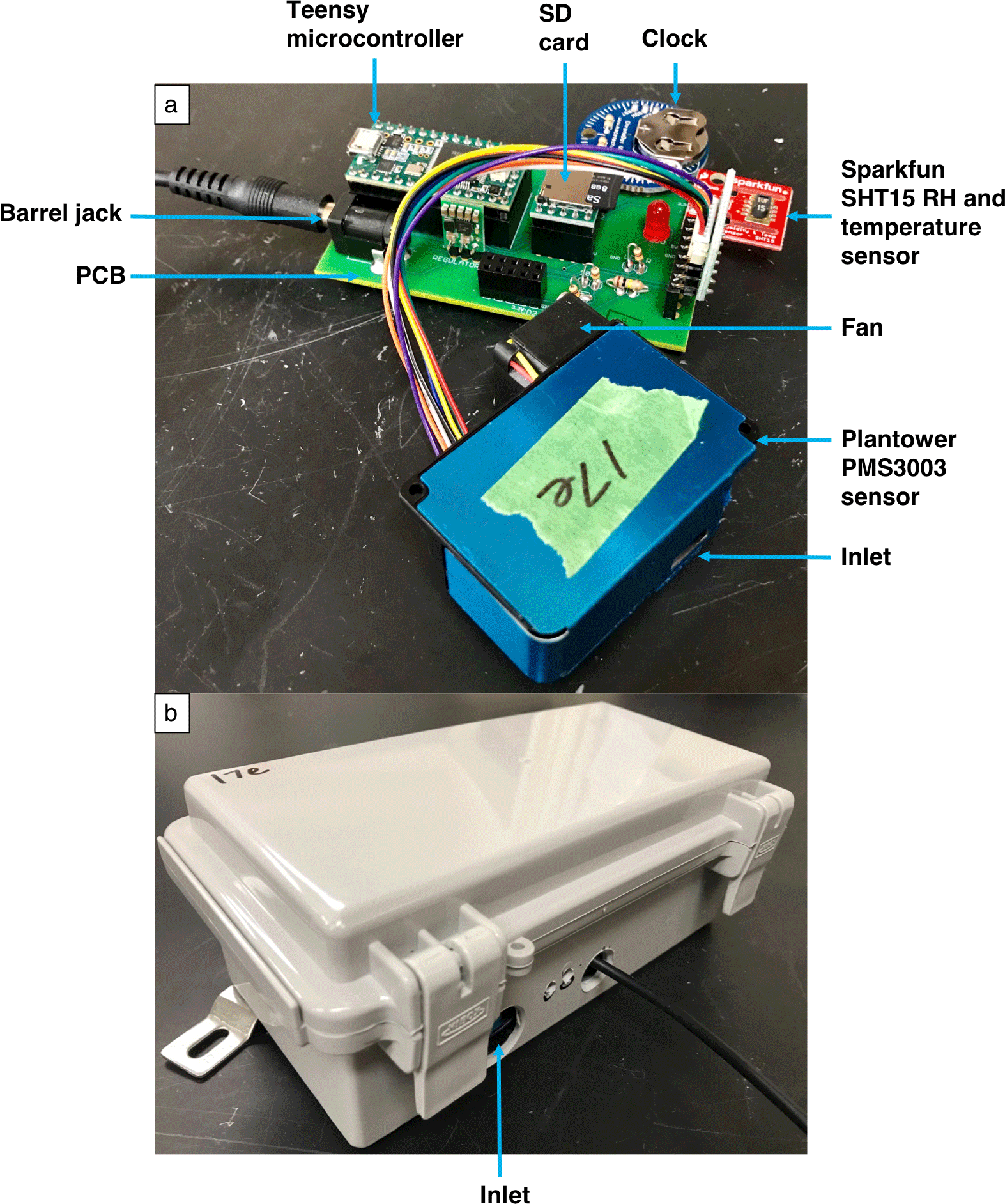
Figure 1(a) The custom-designed printed circuit board (PCB) and its components for the Plantower PMS3003 sensor packages. (b) Electrical box housing all components for outdoor sampling.
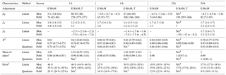
Table 1Summary statistics for 1 h averaged measurements (mean ± SD (range)) at the three sampling locations. Reference monitors at the sampling locations are indicated with bold font. The dates are formatted month/day/year.
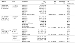
∗ All the PMS3003 sensor packages and the E-BAM were shut down between 3 and 12 March for maintenance.
2.2 Field deployment
Three field campaigns were conducted to evaluate the performance characteristics of Plantower PMS3003 sensors and to explore the potential impacts from artifacts such as RH and temperature on sensors' PM2.5 measurements (Table 1). Two sites were in Durham County, NC, representing suburban environments with low ambient PM2.5 concentrations. The other study site was in Kanpur, Uttar Pradesh, India, representing an urban-influenced environment. The data from Kanpur were subset into the monsoon season with moderately high PM2.5 concentrations and the post-monsoon season with high PM2.5 concentrations.
2.2.1 Low-concentration region: Durham and Research Triangle Park (RTP), NC
The first measurement campaign in the low-concentration region was on the rooftop of the Fitzpatrick Center, a three-story building located on the Duke University West Campus in Durham, NC (latitude 36.003350, longitude −78.940259). The sampling location lies in close proximity to the 28.5 km2 Duke Forest and approximately 3.5 km from the Durham downtown and 4.5 km from the Durham National Guard Armory monitoring station (latitude 36.0330, longitude −78.9043). This study location is also about 950 m southwest of the Durham Freeway, which had an annual average daily traffic of 43 000 vehicles as of 2015 (North Carolina Department of Transportation, 2015). No known principle point source emissions are located in the surrounding area. The 3-year average (2013–2015) for PM2.5 concentrations reported by the Durham National Guard Armory monitoring station was 12 µg m−3, and the reported 98th percentile daily average from 2013 to 2015 was 18 µg m−3 (North Carolina Department of Environmental Quality, 2017). At the Duke site, five Plantower PMS3003 sensors (labeled PMS3003-1 through PMS3003-5) were compared to a collocated environmental β attenuation monitor E-BAM-9800 (Met One Instruments). Unlike its more advanced counterpart BAM-1020 (Met One Instruments), the E-BAM-9800 is not currently a U.S. EPA-designated FEM for PM2.5 mass concentration continuous monitoring, although it is ideal for rapid deployment because of its portability and its ability to accurately track FRM or FEM results with proper operation and regular maintenance (Met One Instruments, 2008). The hourly values reported by the E-BAM (mg m−3) were used in the analyses. The E-BAM's sporadic negative values caused by low actual ambient concentrations (such as below 3 µg m−3) were replaced with 0 µg m−3 in this study. The sensor packages were strapped to the E-BAM tripod and operated in a collocated manner for a period of 50 days from 1 February to 31 March 2017 (all the sensor packages and the E-BAM were shut down between 3 and 12 March for maintenance). Over the course of the deployment, PMS3003-1 was disconnected between 14 and 21 February because of power supply issues, and this situation rendered PMS3003-1 data 86 % complete.
The second ambient test in the low-concentration region was performed at the U.S. EPA's Ambient Air Innovation Research Site (AIRS) on its RTP campus, NC (latitude 35.882816, longitude −78.874471) about 16 km southeast of the Duke site. The ambient PM2.5 mass concentrations in the RTP region are normally well under 12 µg m−3 (Williams et al., 2003). A Thermo Scientific 5030 SHARP (synchronized hybrid ambient real-time particulate monitor) monitor (U.S. EPA PM2.5 FEM) was operated by the U.S. EPA Office of Research and Development (ORD) and two Teledyne API T640 PM mass monitors (U.S. EPA PM2.5 FEM) were operated by the U.S. EPA Office of Air Quality Planning and Standards (OAQPS). The SHARP monitor is a hybrid of a high-sensitivity nephelometer using 880 nm infrared light-emitting diodes (IREDs) and a BAM. The SHARP continuously calculates the ratios of dynamically time-averaged beta concentrations to dynamically time-averaged nephelometer concentrations and continuously employs these ratios as correction factors to adjust the raw 1 min averaged nephelometer readings. The corrected nephelometric concentrations are reported as 1 min SHARP measurements in micrograms per cubic meter (Thermo Fisher Scientific, 2007). The T640 monitor, first introduced in 2016, is one of the latest additions to the list of approved U.S. EPA PM2.5 FEM monitors. The T640 is essentially an optical aerosol spectrometer that uses light scattering to measure particle diameters in 256 particle size classes over the 0.18–20 µm range at the single-particle level. The 256 size classes are subsequently combined into 64 channels for mass calculation with proprietary algorithms. The light source used by the T640 monitor is polychromatic (broadband) light. Compared to traditional monochromatic laser scattering approaches, the polychromatic light approach provides more robust and accurate measurements with significantly less noise, especially over the particle size range of 1 to 10 µm (Teledyne Advanced Pollution Instrumentation, 2016). The T640 reports 1 min resolution results in micrograms per cubic meter. The SHARP and one of the T640 units (T640_Shelter) were installed inside an ORD mobile laboratory and an OAQPS shelter, respectively, with roof penetration while the other T640 unit (T640_Roof) was installed inside an outdoor enclosure with heating, ventilation, and air conditioning (HVAC) control on the rooftop of the OAQPS shelter. Three PMS3003 sensor packages from the Duke site (labeled PMS3003-1 through PMS3003-3) were attached to the rail on top of the ORD mobile laboratory approximately 3 to 4 m above the ground. The SHARP inlet and the sensor packages' inlets were only about a meter apart. The two T640 inlets were situated on the rooftop of the OAQPS shelter, within about 30 m of the sensor packages' inlets. The inlets of these instruments were positioned roughly at the same height above ground. Over the course of the 32-day field project (30 June to 31 July 2017), all the instruments' data completeness was 100 % except that of SHARP (99 %). The slightly incomplete SHARP data stemmed from the removal of midnight concentration spikes (at approximately 01:00 to 01:10 EDT, eastern daylight time) due to the daily filter tape advancement.
2.2.2 High-concentration location: Indian Institute of Technology Kanpur (IIT Kanpur) study site
Identical to the setup at the Duke site, the third field evaluation involving two PMS3003 sensors (labeled PMS3003-6 and PMS3003-7) alongside an E-BAM was carried out on the rooftop of the Center for Environmental Science and Engineering inside the campus of IIT Kanpur (latitude 26.515818, longitude 80.234337). The center is a two-story building (roughly 12 m above the ground level) that lies approximately 15 km northwest of downtown Kanpur. The institute is located upwind of Kanpur and away from major roadways, industrial sites, and dense residential communities; therefore it has comparatively low PM2.5 concentrations (Villalobos et al., 2015). Kanpur is a heavily polluted industrial city on the Indo-Gangetic Plain with a large urban area of dense population (approximately 2.7 million) (Villalobos et al., 2015). Various small-scale industries, a coal-fired power plant (Panki Thermal Power Station), indoor and outdoor biomass burning, heavy vehicles on the Grand Trunk Road (a major national highway) running through Kanpur, fertilizer plants, and refineries are the prime contributors to air pollution (Shamjad et al., 2015; Villalobos et al., 2015). The local climate is primarily defined as humid subtropical with extremely hot summers and cold winters (Ghosh et al., 2014). The monsoon season (June to September) is documented to have lower PM2.5 concentrations than the post-monsoon season (October and November) (Bran and Srivastava, 2017). The two sensor packages were first deployed at the study site on 8 June 2017 for approximately 22 days (early monsoon), and then on 23 October 2017 for approximately 25 days (post-monsoon). Since these two sensor units were not embedded with temperature and RH sensors, the temperature and RH data (available as 15 min averages) were simultaneously collected from an automatic weather station, roughly 500 m away from the study site and 2 to 3 m above the ground. Throughout the sampling periods, error-flagged E-BAM measurements (including delta temperature set point exceeded, flow failure, abnormal flow rate, beta count failure) during the operation were excluded from the analyses for quality assurance purposes, and this caused the E-BAM data to be 85 % and 93 % complete for monsoon and post-monsoon seasons, respectively. The two sensor packages had data completeness close to 100 % for both monsoon and post-monsoon seasons. The temperature and RH data from the automatic weather station were only occasionally missing due to power supply issues with an overall 93 % and 99 % completeness for monsoon and post-monsoon seasons, respectively.

Figure 2Flow path for sensor calibrations. Note raw sensor PM2.5 measurements are uncalibrated sensor PM2.5 measurements.
2.3 Sensor calibrations
Sensor PM2.5 measurement adjustments/corrections were made as described in the following three subsections. First, we evaluated the dependence of sensor response on RH (Sect. 2.3.1); if this was significant we adjusted sensor PM2.5 values for RH. Next, we investigated the sensor response dependency on temperature (Sect. 2.3.2); if this was significant we simultaneously adjusted sensor PM2.5 values for temperature and calibrated sensor values based on reference monitors. If this was not significant, we simply applied a calibration based on the reference PM2.5 values and corrected for any nonlinear performance (Sect. 2.3.3). The calibration strategy is shown graphically in Fig. 2.
2.3.1 RH adjustment to sensor PM2.5 measurements
FEMs and research-grade PM analyzers typically control for RH by dynamically heating the sample air inlet. Our sensor packages, similar to many low-cost designs, are not equipped with any heaters or conditioners to reduce RH impact. Therefore, the RH can significantly bias the PM2.5 mass concentrations reported by our sensor packages. The effect of RH on the mass of atmospheric aerosol particles has been well documented for decades. Sinclair et al. (1974) showed that there was a 2- to 6-fold increase in the mass of particles, depending on the properties of the particles, as the RH reached 100 %. Waggoner et al. (1981) also showed that RH above roughly 70 % can enhance scattering coefficients of hygroscopic or deliquescent particles in various locations in the western and midwestern US due to the growth of these particles associated with water uptake. Zhang et al. (1994) described the calculated scattering efficiencies of ammonium sulfate in the Grand Canyon as a function of RH with empirical Eq. (1). This equation was later employed by Chakrabarti et al. (2004) to predict the effect of RH on the relationship between the nephelometric personal monitors' PM2.5 mass concentration measurements and the results of a reference monitor (BAM). They found that the model agreed quite well with the field data collected from both their study and a previous study (Day and Malm, 2001). An identical equation was also among a wide variety of approaches assessed by Soneja et al. (2014) to adjust nephelometric personal monitor PM2.5 readings for the RH impact. We believe lessons learned from these previous studies can be directly applied to RH adjustments for low-cost nephelometric sensors' PM2.5 measurements in the present study by using Eq. (1):
Ordinary least-squares (OLS) regressions were conducted to obtain the empirical regression parameters a and b in Eq. (1), where the dependent variable was the RH correction factors calculated as the ratio of PMS3003 PM2.5 mass concentrations averaged across all the sensor package units to the corresponding reference monitor concentrations at each point in time at a sampling location, and the independent variable was the entire term. The RH was the measurements averaged across all the embedded Sparkfun SHT15 RH and temperature sensors at each point in time for the calibration models of Duke University and EPA RTP study sites, and the measurements from the automatic weather station for the models of the IIT Kanpur study site. The empirical equations derived were used to compute the RH correction factor for a given RH at the sampling sites. The RH interferences were compensated for by dividing each individual raw PMS3003 PM2.5 mass concentration for a given RH by the RH correction factor yielded for that RH (Eq. 2):
We only performed the RH adjustments when the fitted models for any of the sampling locations over any time-averaging interval had at least a moderate coefficient of determination (R2≥0.40). The slightly high correlation cutoff value was implemented in this study to ensure that the RH corrections can effectively lower the error of the low-cost sensor PM2.5 measurements. Despite the similarity of the general shape of correction factor curves in different studies, the detailed behaviors of aerosols diverged greatly due to considerable difference in particle chemical composition and diameter (Waggoner et al., 1981; Zhang et al., 1994; Day and Malm, 2001; Chakrabarti et al., 2004; Soneja et al., 2014). In a previous study (Day and Malm, 2001), aerosol mass at some locations increased continuously above a relatively low RH (such as 20 %), whereas at other locations it exhibited a distinct deliquescent behavior (i.e., aerosol water uptake occurred at a relatively high RH). Even for aerosols showing deliquescent behavior, the observed deliquescence RH (RH threshold) varies from study to study. Soneja et al. (2014) also found underestimation of PM concentrations (correction factors less than 1) below 40 % RH. Because of these uncertainties, we conducted RH adjustments across the entire range of recorded RH without incorporating an RH threshold. Additionally, the RH adjustments in this study were always performed separately from and prior to either temperature adjustments or reference monitor adjustments.
2.3.2 Temperature adjustment to sensor PM2.5 measurements
The Akaike's information criterion (AIC) is a widely used tool for model selection to address the fact that including additional predictors may overfit the data (Crawley, 2017). It was used to determine the significance of the temperature term in the PMS3003 calibration models for all the study locations at various averaging times. The AIC penalizes more complex models based on the number of parameters fit in that model. A lower AIC when comparing two models for the same data set indicates a better fitting model. In a linear regression model, an AIC difference between two models of less than or equal to 2 indicates that the more complex model does not improve predictive performance. Therefore, the simpler model should be adopted. We specifically compared the AIC value of a multiple linear regression model, which included both the reference monitor measurement and temperature as predictor variables and without considering an interaction term (i.e., Eq. 3) to the value of a univariate linear regression model with only the reference monitor measurement as a predictor variable (i.e., Eq. 4). We performed the temperature adjustments using Eq. (5) only when the AIC indicated that the temperature predictor was significant in the calibration model (i.e., ).
The temperature was the measurements averaged across all the embedded Sparkfun SHT15 RH and temperature sensors at each point in time for the models of Duke University and EPA RTP study sites and the measurements from the automatic weather station for the models of the IIT Kanpur study site. Since the RH adjustments in this study were always performed first, the PMS3003 PM2.5 concentration in Eqs. (3) and (4) were RH-adjusted PMS3003 PM concentrations when RH adjustments were significant and were otherwise raw PMS3003 PM2.5 concentrations. Additionally, temperature adjustments and reference monitor adjustments were always conducted simultaneously when the temperature predictor was significant because Eq. (3) consists of both the reference monitor concentration and temperature terms as independent variables. The AIC values for models with 24 h data are not reported in the present study as 24 h observations generally have limited statistical power to determine the significance of temperature in the models.
2.3.3 PM2.5 sensor calibrations based on reference monitor values
The most basic calibration is a direct comparison with reference monitor measurements. We derived reference instrument calibration equations (Eq. 4) by fitting a linear least-squares regression model to each pair of PMS3003 (dependent variable) and collocated reference instrument's PM2.5 mass concentrations (independent variable). The PMS3003 PM2.5 values were RH-adjusted concentrations when RH adjustments were significant and were otherwise raw concentrations. Each PMS3003 measurement was subsequently calibrated using Eq. (6).
When the relationship between PM2.5 mass concentrations of reference monitors and PMS3003 sensors was nonlinear, PM2.5 sensor calibration equations based on reference monitor values in a quadratic form (Eq. 7) were used to describe the nonlinear performance and each PMS3003 measurement was subsequently calibrated using Eq. (8) since calibrated values should always be on the left side of the axis of symmetry of the parabola with a2<0. The AIC values (discussed in Sect. 2.3.2), and the root-mean-square errors (RMSEs) (Eq. 9) were used in combination to assess the goodness of fit and accuracy of the two model approaches (i.e., univariate linear and quadratic models) as a function of integration times.
Here n is the number of observations, is the calibrated PMS3003 PM2.5 mass concentrations, and yi is the reference monitor PM2.5 mass concentrations.
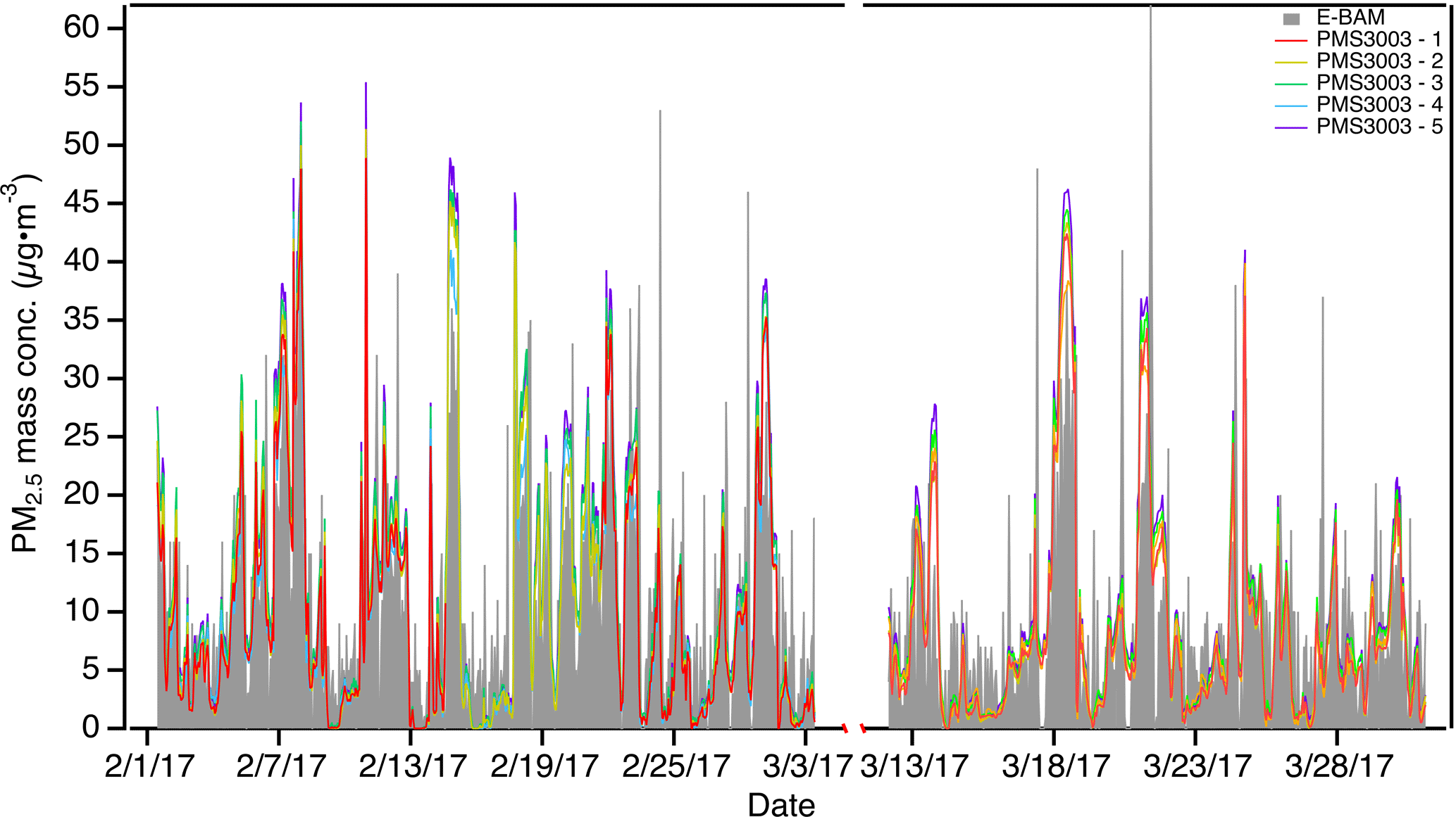
Figure 3Comparison of hourly PM2.5 mass concentrations between the E-BAM and the five uncalibrated PMS3003 sensor packages between 1 February and 31 March 2017 at Duke University.
2.4 Sensor performance metrics
Metrics such as the intercept, slope, and coefficient of determination (R2) obtained from OLS models of sensor outputs with reference instrument measurements are widely used to evaluate sensor performance (Holstius et al., 2014; Gao et al., 2015; Wang et al., 2015; Jiao et al., 2016; Cross et al., 2017; Kelly et al., 2017; Zimmerman et al., 2018). In this study, all the R2 values in figures represent regression coefficients of the (calibration) equations while all the R2 values in tables represent regression coefficients between the calibrated sensor and reference measurements. To date, only a few studies have attempted to compute parameters other than R2 to gauge the overall performance of low-cost sensor technologies. They typically focus on the RMSE (Holstius et al., 2014; Cross et al., 2017; Zimmerman et al., 2018), the mean absolute error (MAE) and the mean bias error (MBE) (Cross et al., 2017; Zimmerman et al., 2018), and normalized residuals (Sousan et al., 2017; Kelly et al., 2017). In addition to the intercept, slope, and R2, we also used ratios of the calibrated PMS3003 PM2.5 mass concentrations to reference monitor values to examine sensors' post-calibration performance. From this set of ratios, we calculated an average ratio and 1 standard deviation (SD), which are defined as mean of ratios and error for each sensor unit, respectively. The mean of ratios should be close to 1 after calibration, and we would expect the error of any PM2.5 mass concentration reported by a particular PMS3003 unit to be within ±1 SD × 100 % for 68 % of the time. Knowing the performance of calibrated PMS3003 sensors is particularly important for understanding these sensors' potential for future applications such as investigating the source and transport patterns of PM in an urban environment or examining the effectiveness of certain PM abatement strategies.
While longer averaging times (i.e., ≥24 h) typically smooth out noisy signals and result in enhanced sensor performance, shorter averaging times (i.e., hours or minutes) are of growing interest, particularly in the field of exposure assessment (Williams et al., 2017). Similar to Williams et al. (2017), we also evaluated sensor performance over a wide range of time-averaging intervals, namely 1 min (for the EPA RTP – the only site where 1 min reference data were available), 1 h, 6 h, 12 h, and 24 h. The purpose of such an examination is to better understand the tradeoff between errors and averaging times when using this type of sensor so that data accuracy and precision can be weighed against the need for highly time-resolved data for various desirable research or citizen science applications.
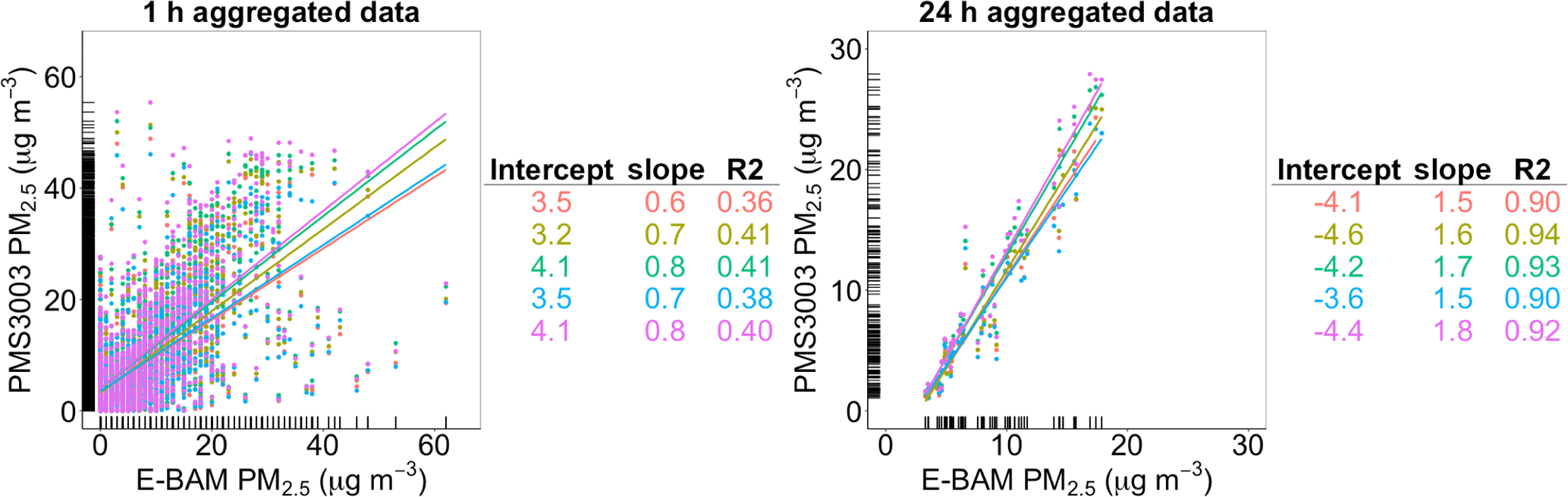
Figure 4Linear regressions between aggregated PM2.5 mass concentrations (µg m−3) of the E-BAM and the five uncalibrated PMS3003 sensors at 1 and 24 h time intervals from 1 February to 31 March 2017 at Duke University (6 and 12 h results not shown). Marginal rugs were added to better visualize the distribution of data on each axis.
Table 2Summary of sensor performance characteristics for the five PMS3003 PM2.5 measurements at 1, 6, 12, and 24 h time intervals from 1 February to 31 March 2017 at Duke University. The fit coefficients for the calibration models are provided. The R2, mean of ratios, and error are performance characteristics for the calibrated sensor PM2.5 measurements in comparison with reference values. The results are displayed in mean (range) format. Note the mean statistics were obtained by fitting the models to the PMS3003 PM2.5 measurements averaged across all five sensor package units at each point in time.
β0: intercept. β1: coefficient for
E-BAM. β2: coefficient for temperature (T). 1 Mean of
ratios of calibrated PMS3003 to E-BAM PM2.5 concentration. 2 Defined as 1 SD
of ratios
of calibrated PMS3003 to E-BAM PM2.5 concentration.
3.1 Duke University rooftop low ambient PM2.5 concentration environment with E-BAM as the reference monitor
3.1.1 PM2.5 concentration, RH, and temperature on a 1 h scale
Table 1 shows the summary statistics for 1 h averaged measurements at Duke University from 1 February to 31 March 2017. The 1 h E-BAM PM2.5 measurements averaged 9±9 µg m−3. The hourly PM2.5 averages of the uncalibrated sensors were close to those of the E-BAM and had little intra-sensor variability. We calculated the coefficient of variation (defined as the ratio of the SD and the mean of the PM2.5 readings from the five replicate PMS3003 sensors) as an indicator of sensor precision, which yielded 10 %, indicating the relatively high precision of the PMS3003 model. RH and temperature averaged 45±19 % and 15±8 ∘C, respectively. Figure 3 compares the 1 h E-BAM PM2.5 mass concentrations to the results of the five uncalibrated sensors. Overall, the uncalibrated PMS3003 measurements followed the trend in ambient PM2.5 concentrations and were very responsive to most sudden spikes in concentrations. However, the sensors tended not to track the E-BAM well below ∼10 µg m−3.
3.1.2 PMS3003 performance characteristics on various timescales
Correlations among the five uncalibrated PMS3003 units were high (R2=0.98–1.00) on a 1 h timescale even under low ambient PM2.5 concentrations with slopes averaging 1±0.1 and negligible intercepts averaging 0.3±0.3 (Fig. S1 in the Supplement), suggesting excellent intra-PMS3003 precision. Regressions of the uncalibrated 1 and 24 h PM2.5 measurements from the five PMS3003 units versus the corresponding E-BAM PM2.5 values indicate that different PMS3003 sensor units generally had similar calibration factors (i.e., intercept and slope values) on the same timescale (Fig. 4). Comparing across the time-averaging interval spectrum (Table 2), the calibration factors on different timescales were consistent, with the exception of 1 h results. Raw 1 h aggregated PMS3003 PM2.5 concentration measurements correlated only moderately with the corresponding E-BAM data, with a mean R2 of 0.40 (range: 0.36–0.41). When the averaging time increased from 1 to 6 h, the R2 showed a marked improvement (mean: 0.80, range: 0.77–0.82). When the averaging time further rose to 12 h and from 12 to 24 h, although still accompanied by improvements in R2 (mean: 0.84 and 0.93, respectively), the magnitudes of the improvements were considerably smaller than the one seen from 1 to 6 h.
The SCAQMD (2017a) also field-tested three Plantower PMS3003 units (Laser Egg sensors) alongside an FEM (BAM-1020, Met One Instruments) over a study period of similar length (roughly 2 months) with similar ambient PM2.5 concentrations (1 h PM2.5 range: 0–40 µg m−3) in Riverside, CA, although the data were presented differently (with reference and sensor measurements on the y and x axes, respectively) and thus the values of calibration factors cannot be directly compared to our study. The SCAQMD study demonstrated the calibration factors on a 1 h scale (intercept: 5.9–6.3, slope: 0.50–0.57) were virtually the same as the values on a 24 h scale (intercept: 6.0–6.3, slope: 0.48–0.57). This observation is in contrast to our finding in which 1 h results (intercept: 3.2–4.1, slope: 0.64–0.79) differed dramatically from the 24 h values (intercept: −4.6 to −3.6, slope: 1.5–1.8). This discrepancy might stem from the use of different reference instruments in the two studies. While both instruments use beta attenuation as the measurement principle, the accuracy of BAM-1020 (FEM) for 1 h measurements in the SCAQMD study is significantly better than that of the E-BAM-9800 (research grade) in our study. This may also account for the higher R2 on a 1 h scale in the SCAQMD study (around 0.58).
Table 2 shows that the pattern of errors was aligned with our expectation, with each of the four time integration values having successively more accurate post-calibration PMS3003 PM2.5 concentrations than all the previous time integration values (i.e., the error decreased as the averaging time increased). Furthermore, the steep gradient at which the mean error reduced over averaging time (from 201 % for 1 h to 15 % for 24 h) was unusual and most likely caused by E-BAM's poor signal-to-noise ratio at low concentrations with short real-time average periods. This finding points out that the precision of reference monitors is a critical factor in sensor evaluation, as discussed in detail in Sect. 3.2.2. It should be noted that the strong correlation on a 6 h scale (R2 mean = 0.8) did not translate into a low error (mean: 53 %). This observation emphasizes the downside of overreliance on the correlation in the examination of sensor performance.
Figure S2 displays the relationship between the PMS3003-to-E-BAM PM2.5 ratio and RH on a 1 h scale at Duke University. There was no apparent pattern of fractional increase in PM2.5 weight measured by uncalibrated PMS3003 sensors with RH. Fitting the empirical RH correction factor model (i.e., Eq. 1 in Sect. 2.3.1) to these field data resulted in an R2 close to 0. Examination of patterns and model fitting at longer averaging time intervals (i.e., 6, 12, and 24 h) yielded comparable results (not shown). These findings are indicative of the negligible impact of RH on PMS3003 PM2.5 responses at Duke University. This lack of RH interference is believed to stem from a combination of infrequently high RH conditions during the winter months (only 12.5 % and 4.0 % of the entire time greater than 70 % and 80 %, respectively) and large measurement error inherent in the E-BAM under low PM2.5 concentrations.
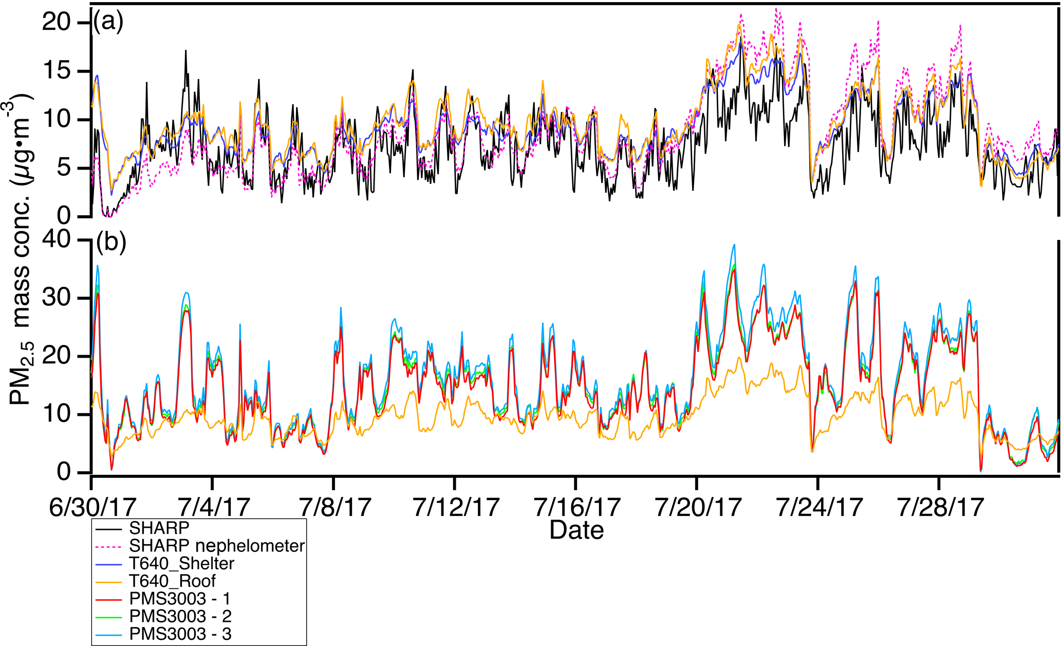
Figure 5Comparison of hourly aggregated PM2.5 mass concentrations (µg m−3) (a) among the SHARP, the SHARP's nephelometer, the two T640 sensors (one unit sitting on the roof, “T640_Roof”; the other unit installed in the OAQPS shelter, “T640_Shelter”), from 30 June to 31 July 2017 at U.S. EPA RTP, and (b) between the T640 sitting on the roof (T640_Roof) and the three uncalibrated PMS3003 sensor packages during the same period at the same location.
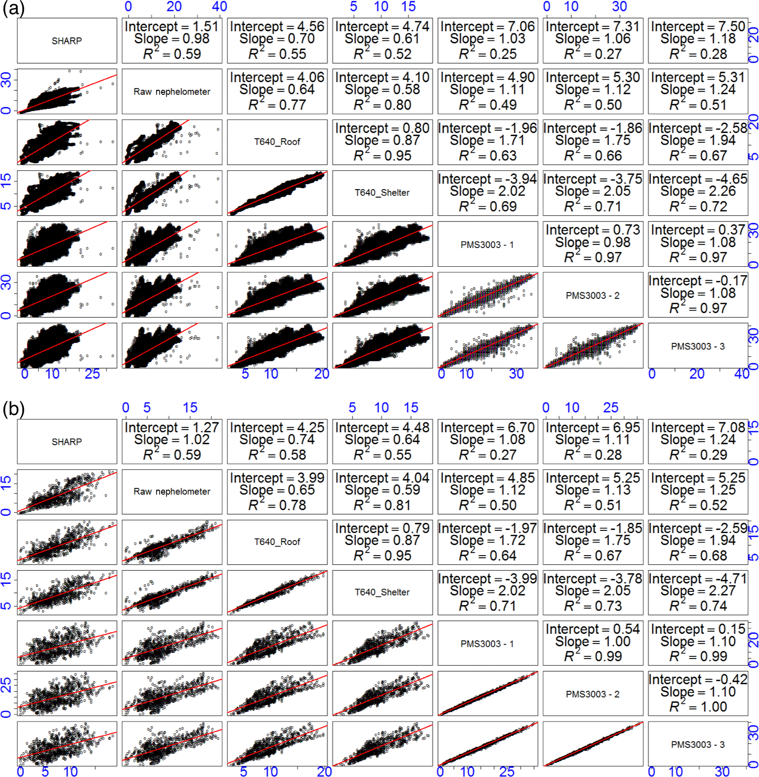
Figure 6Pairwise correlations between (a) 1 min aggregated PM2.5 mass concentrations (µg m−3) and (b) 1 h aggregated PM2.5 mass concentrations (µg m−3) of the SHARP, the SHARP's nephelometer, the two T640 sensors, and the three uncalibrated PMS3003 sensor packages between 30 June and 31 July 2017 at U.S. EPA RTP. In both panels (a) and (b), the upper right set of panels includes the intercept, slope, and R2 of linear regression models using the ordinary least-squares (OLS) method; the lower left set of panels shows the linear regression lines superimposed on pairwise plots.
Table S1 demonstrates that the AIC differences between the calibration models with only a true PM2.5 concentration term and the models incorporating an additional temperature term were greater than 2 for only the 1 h aggregated data, implying the calibration model with an added temperature term was significantly better than its simpler counterpart only on the 1 h scale. Therefore, the temperature adjustment was performed only for 1 h averaged PMS3003 responses at the Duke University study site. Counterintuitively, Table 2 shows that the temperature correction worsened the sensor performance by bringing the mean of ratios down from 0.97 to 0.90 and by bringing the error up from 201 % to 207 %. The deterioration in performance was likely to arise from large measurement error inherent in the E-BAM under low PM2.5 concentrations.
3.2 RTP low ambient PM2.5 concentration environment with SHARP and T640 as the reference monitors
Following sampling on the rooftop at Duke, we moved three PMS3003 units (labeled PMS3003-1 through PMS3003-3) from the Duke University study site to the U.S. EPA AIRS on its RTP campus and further compared these three units to the more accurate and precise regulatory FEMs (i.e., SHARP and two T640s). This allowed us to determine whether much of the poor performance of the Plantower PMS3003 sensors, the indistinct RH effects on the PMS3003 PM2.5 measurements, and the unsuccessful temperature corrections to the PMS3003 PM2.5 values were attributable to the inferior precision of the E-BAM.
3.2.1 PM2.5 concentration, RH, and temperature on a 1 h scale
Figure 5a shows 1 h time series data from all the reference monitors including the SHARP's embedded nephelometer and Fig. 5b juxtaposes the T640_Roof and the three uncalibrated PMS3003 units' PM2.5 measurements at 1 h time resolution. Table 1 indicates that the 1 h averaged ambient PM2.5 levels at the U.S. EPA RTP (9–10 µg m−3) matched those at Duke University (9 µg m−3). However, Fig. 5a depicts smaller ranges of ambient PM2.5 concentrations than were measured at Duke University. Table 1 indicates that the SD (less than 4 µg m−3) and maximum PM2.5 concentration (less than 20 µg m−3) at the EPA RTP were significantly lower than at Duke University (9 and 62 µg m−3 for SD and maximum, respectively). These comparisons imply that the RTP sampling location had overall lower ambient PM2.5 concentrations and was consequently more challenging for low-cost sensors than the Duke University sampling site. During the measurement period, the mean RH and temperature were 64±22 % and 30±7 ∘C, respectively. The higher average RH level at the EPA RTP than at Duke University (45±19 %) accentuated the RH interference in the PMS3003 PM2.5 measurements, as seen in Sect. 3.2.3.
3.2.2 PMS3003 performance characteristics on various timescales prior to adjustment for meteorological parameters
Figure 6a–b graphically and statistically summarize the pairwise correlations among all the instruments' 1 min aggregated and 1 h aggregated PM2.5 mass concentrations, respectively. The R2 and calibration factors among all the instruments on 1 min and 1 h scales were similar. The PMS3003 sensors were well correlated with one another (R2=0.97), the two T640 sensors (R2≥0.63), and the SHARP's embedded nephelometer (R2≥0.49) even for 1 min aggregated data at exceptionally low ambient PM2.5 levels. In contrast, the 1 min or 1 h PMS3003–SHARP correlations (R2≥0.25) were poor and worse than the 1 h PMS3003–E-BAM correlations (R2≥0.36) at the Duke site. Additionally, the SHARP had only moderate correlations with the two T640 sensors (R2≤0.58) or the SHARP's embedded nephelometer (R2=0.59) even though both the SHARP and T640 are US-designated PM2.5 FEMs and the SHARP readings take into account its raw nephelometer values.
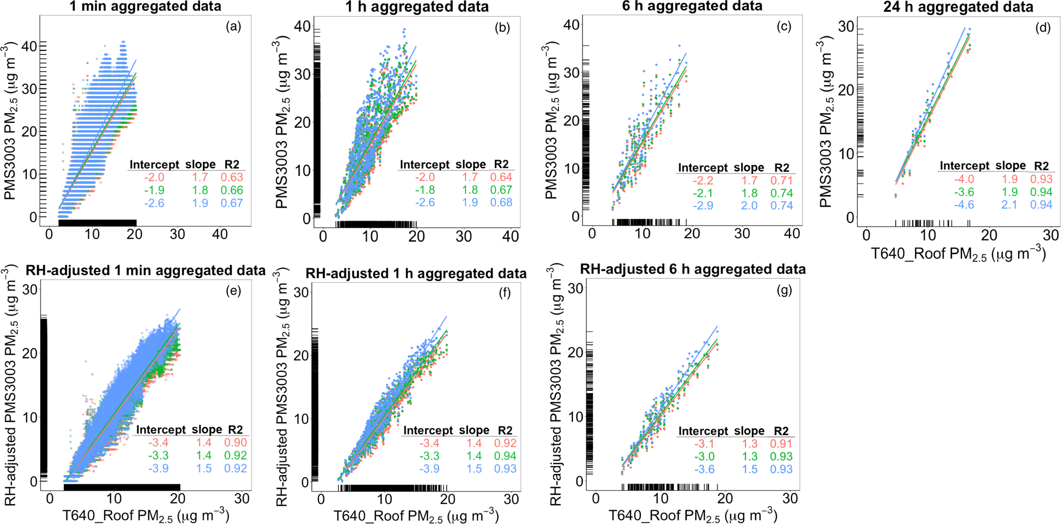
Figure 7Linear regressions between aggregated PM2.5 mass concentrations (µg m−3) of the T640 sitting on the roof (T640_Roof) and the three PMS3003 sensors from 30 June and 31 July 2017 at U.S. EPA RTP. In panels (a)–(d), the PMS3003 readings are raw values at 1 min, 1 h, 6 h, and 24 h, respectively (12 h results are not shown). In panels (e)–(g), the PMS3003 readings are RH-adjusted values at 1 min, 1 h, and 6 h, respectively. Marginal rugs were added to better visualize the distribution of data on each axis. Note the rug on the y axis in (a) is sparse because 1 min raw PMS3003 PM2.5 measurements are recorded as integers.
While the common optically based principles of operation shared by T640 (and nephelometer) and PMS3003 could partially explain the stark performance contrast between the SHARP and T640 (and nephelometer), the lower reported precision of the beta-attenuation-based approach with a 24 h average of ±2 µg m−3 for SHARP than the T640 with a 1 h average of ±0.5 µg m−3 in low ambient PM2.5 concentration environments appears to be the root cause (Thermo Fisher Scientific, 2007; Teledyne Advanced Pollution Instrumentation, 2016). A previous study by Holstius et al. (2014) demonstrated the poor performance of BAM-1020 in a comparably low-concentration environment in Oakland, CA. They used both statistical simulation based on the true ambient PM2.5 distribution and the measurement uncertainty of BAM-1020 (1 h average: ±2.0–2.4 µg m−3) provided by the manufacturer (Met One Instruments) and field test results to show that an R2 of ∼0.59 is as correlated as one would expect from the 1 h measurements of a pair of collocated BAM-1020 sensors. In contrast to the moderate intra-BAM-1020 correlation (∼0.59) reported by Holstius et al. (2014), the two collocated T640 instruments yielded an ideal R2 of 0.95 (Fig. 6), which suggests a significantly smaller measurement error in the T640 than in the BAM-1020. The SHARP is known to derive its reported values by dynamically adjusting its embedded nephelometer readings based on its BAM measurements. In other words, the SHARP performance was adversely affected by the low precision of its embedded BAM at low ambient PM2.5 levels. All these observations seem to imply that beta-attenuation-based monitors might be unfavorable for low-cost particle sensor evaluation at the low concentrations typically present in the US. U.S. EPA FEMs are valid for 24 h PM2.5 measurements rather than for 1 h measurements (Jiao et al., 2016). An inappropriate selection of reference monitors might prejudice the overall performance of low-cost sensors, particularly for time resolutions finer than 24 h.
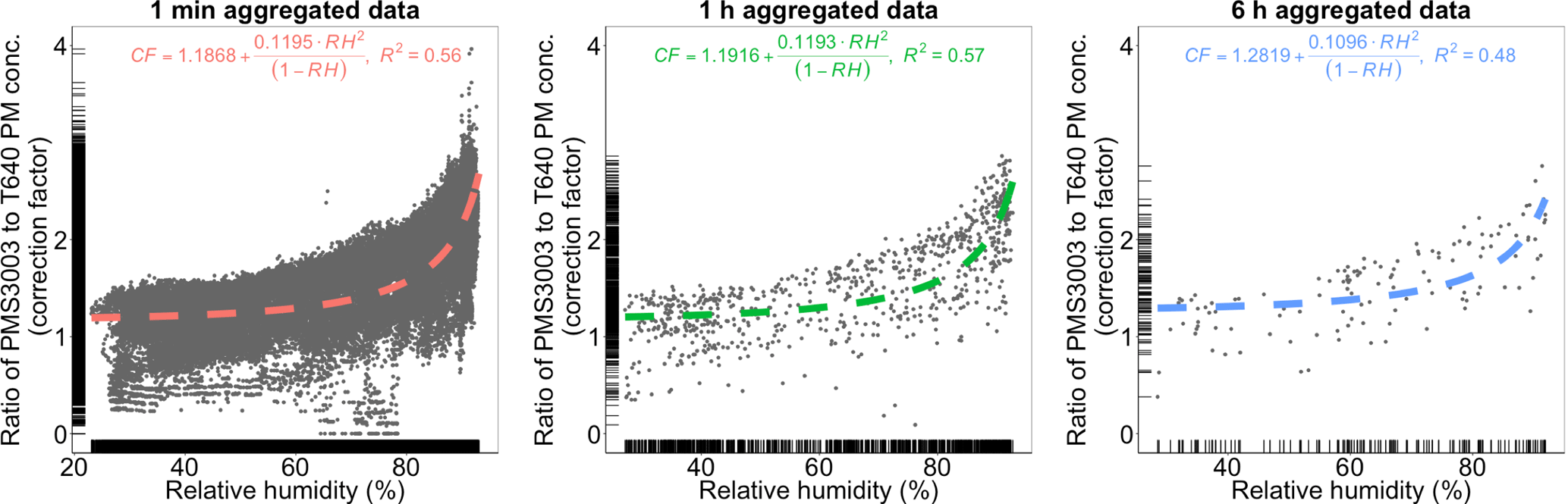
Figure 8Fractional increase in PM2.5 weight measured by the uncalibrated PMS3003 sensors with respect to RH at 1 min, 1 h, and 6 h time intervals from 30 June and 31 July 2017 at U.S. EPA RTP. RH (%) and PMS3003 PM2.5 concentrations (µg m−3) are arithmetic means averaged across all the three PMS3003 sensor packages at each point in time. The fitted RH adjustment equations and curves were superimposed on the plots. Marginal rugs were added to better visualize the distribution of data on each axis. The results of 12 and 24 h aggregated data are not shown as their patterns are relatively indistinct.
The T640 sitting on the roof (T640_Roof) was chosen over the SHARP and the other T640 unit (T640_Shelter) as the reference monitor because (1) the T640 as a US-designated PM2.5 FEM is better for sensor evaluation at low concentrations than a SHARP and (2) the T640_Roof had slightly lower correlations with the sensors than the T640_Shelter, therefore giving conservative estimates of PMS3003 performance. Similar to the Duke University results, comparisons of the data using regression between the same set of instruments in Fig. 7a–d present similar calibration factors across the sensors on the same timescale, therefore indicating the excellent precision of the PMS3003 model. Unlike the analysis of the Duke University data, the calibration factors (prior to adjustments for meteorological parameters) varied little from one averaging timescale to another (Table 3). Despite an appreciable improvement in R2 compared to the Duke University site being found only on the 1 h scale, the accuracy of the T640 calibrated PMS3003 units substantially outperformed their E-BAM calibrated counterparts across the entire averaging time spectrum (Table 3) with the most pronounced difference on the 1 h scale (27 % vs. 201 %). A less dramatic mean error drop from the 1 to 24 h scale at the EPA RTP (27 % to 9 %) compared to what was seen at the Duke University site (201 % to 15 %) highlights the inferior precision of the E-BAM and further undermines its credibility as a reference sensor at low PM2.5 concentrations. It should be noted that the non-normally distributed residuals on 1 min, 1 h, and 6 h scales in Fig. 7a–c indicate that the true ambient PM2.5 concentration term alone was not sufficient to explain the variation in PMS3003 measurements, therefore revealing the likely existence of RH or temperature impacts.
3.2.3 RH adjustment to sensor PM2.5 measurements
Figure 7e–g display the regressions of PM2.5 measurements from the RH-adjusted PMS3003 units versus the T640_Roof on 1 min to 6 h timescales. The empirical equations of the RH correction factors (i.e., Eq. 1) on the corresponding timescales are shown in Fig. 8 and they fitted well with the 1 min to 6 h aggregated data (R2≥0.48). The RH adjustment was not implemented to the 12 and 24 h aggregated data because the equation regression fit statistics degraded when evaluating these data, likely because of an insufficient number of observations and stronger smoothing effects at longer averaging time intervals. Aerosols at the EPA RTP generally exhibited smooth and continuous growth above the lowest collected RH rather than distinct deliquescence behavior (Fig. 8). The RH correction factors were roughly 20 % to 30 % above 1 even at the lowest RH (below 30 %), which justifies the decision of conducting RH adjustments across the entire range of recorded RH without incorporating an RH threshold. Despite the promising descriptions of correction factors as a function of RH, wide divergence in the magnitude of correction factors for a given RH exists. This divergence is likely the result of substantial day-to-day variation in the chemical composition of the aerosols (Day and Malm, 2001). A higher fraction of soluble inorganic compounds can contribute to a larger magnitude of RH correction factors (Day and Malm, 2001).
Table 3Summary of sensor performance characteristics for the three PMS3003 PM2.5 measurements at 1 min, 1 h, 6 h, 12 h, and 24 h time intervals. The three PMS3003 instruments were compared to the T640 sitting on the roof from 30 June to 31 July 2017 at U.S. EPA RTP. The temperature (T) correction is only valid for the 1 min to 12 h aggregated data and the RH correction is only valid for the 1 min to 6 h aggregated data. The fit coefficients for the calibration models are provided. The R2, mean of ratios, and error are performance characteristics for the calibrated PMS3003 PM2.5 measurements after the entire suite of indicated adjustments in comparison with reference values. The results are displayed in mean (range) format. Note the mean statistics were obtained by fitting the models to the PMS3003 PM2.5 measurements averaged across all the three sensor package units at each point in time.

β0: intercept. β1: coefficient for
T640. β2: coefficient for temperature (T). 1 Mean of
ratios of calibrated PMS3003 to E-BAM PM2.5 concentration. 2 Defined as 1 SD
of ratios of calibrated PMS3003 to E-BAM PM2.5
concentration.
Intercept and slope under the T640 adjustment define the linear relationship
between the raw PMS3003 (y axis) and T640 PM2.5 measurements
(x axis) while under the RH and T640 adjustments they define the linear
relationship
between the RH-adjusted PMS3003 (y axis) and T640 PM2.5
measurements (x axis).
The RH corrections brought the PMS–T640 correlations to above 0.90 for all 1 min, 1 h, and 6 h aggregated data (see Fig. 7e–g). This significant improvement in R2 implies a major RH influence that can explain up to nearly 30 % of the variance in 1 min and 1 h PMS3003 PM2.5 measurements in addition to the true ambient PM2.5 concentration variable. Figure S3 demonstrates that the PMS3003-to-T640 ratios after the RH corrections were also considerably closer to a strict normal distribution than those with only the FEM corrections (Fig. S4). However, Fig. 7e–g suggest that the PMS3003 PM2.5 measurements were still not in complete agreement with the T640 readings even after the RH adjustments. This discrepancy might stem from variations in aerosol composition described previously or impacts of particle size biases (Chakrabarti et al., 2004), therefore warranting a further step of FEM conversion (adjustment). According to Table 3, the combination of RH and FEM corrections were able to substantially improve the accuracy of PMS3003 PM2.5 measurements by reducing the mean errors to within 12 % even for data at a 1 min time resolution. The ideal normal distribution of PMS3003-to-T640 ratios in combination with the high accuracy and precision of the most finely grained data proves especially beneficial for minimization of exposure measurement errors in short-term PM2.5 health effect studies (Breen et al., 2015) or mapping of intra-urban PM2.5 exposure gradients (Zimmerman et al., 2018).
3.2.4 Temperature adjustment to sensor PM2.5 measurements
The decision to conduct the temperature adjustments to 1 min, 1 h, 6 h, and 12 h aggregated PMS3003 PM2.5 measurements was based on the AIC results in Table S1. Table S1 demonstrates that the AIC values of the calibration models incorporating an additional temperature term were substantially lower than those of the models including only a true PM2.5 concentration term at these levels of temporal resolution, therefore indicating the significance of the temperature variable in the calibration models. The 24 h AIC values are not reported as 24 h observations generally have limited statistical power to determine the significance of temperature in the models.
As shown in Table 3, the temperature corrections (when available) could further reduce the mean PMS3003 PM2.5 measurement errors by no more than 4 %, with the largest reduction in mean errors found in the 12 h averaged data. This marginal improvement stands in marked contrast to that brought about by the RH corrections (up to 17 %), suggesting the triviality of temperature adjustments in the entire suite of calibrations. Nevertheless, the addition of the temperature adjustments succeeded in lowering the mean errors to within 10 % at 1 min, 1 h, and 6 h time resolutions, which were comparable to the value at 24 h time resolution (9 %). Figure S5d also depicts the PMS3003-to-T640 ratios at a 12 h averaging interval after the temperature corrections and shows that these ratios were slightly more normally distributed than those with only the FEM corrections (Fig. S4). As a result, whether to conduct temperature adjustments is contingent upon the error targets, which are further dependent on the performance goals for the desired applications.
3.3 IIT Kanpur high ambient PM2.5 concentration environment with E-BAM as the reference monitor
Low-cost particle sensors are commonly known to exhibit an upward trend in accuracy with increasing ambient PM2.5 concentrations (Williams et al., 2017; Johnson et al., 2018). Moreover, Kanpur presents distinct seasonal variations in the particle size distribution. During the early stage of the monsoon season (June), coarse-mode aerosols are predominant due to the transport of dry dust particles from the western Thar Desert or arid regions to Kanpur. In contrast, during the post-monsoon season, anthropogenic accumulation-mode aerosols transported from the north and northwest dominate over Kanpur (Sivaprasad and Babu, 2014; Li et al., 2015; Bran and Srivastava, 2017). We explored how the variability in the ambient PM2.5 concentrations and the particle size distribution affected the low-cost PM sensors' performance and calibration curves relative to the reference monitor (E-BAM in our study).
3.3.1 PM2.5 concentration, RH, and temperature on a 1 h scale
Table 1 shows that Kanpur had significantly higher ambient PM2.5 levels for a 1 h averaging period during the post-monsoon season (116±57 µg m−3) than during the monsoon season (36±17 µg m−3). This seasonal increase in ambient PM2.5 concentrations is aligned with our expectation and can be attributed to diminished wet scavenging by precipitation, a shallow boundary layer (mixing height), and lower ventilation coefficients (wind speed) during the post-monsoon season (Gaur et al., 2014). While only moderately high ambient PM2.5 levels were found during the Kanpur monsoon season, they were substantially higher than those measured at the Duke University site (9±9 µg m−3). The field tests in this study provided a wide range of ambient PM2.5 levels spanning from high (Kanpur post-monsoon season), moderate (Kanpur monsoon season), to low (Duke University site). This PM2.5 concentration range coupled with the same type of reference monitor (E-BAM) is ideal for constructing empirical error curves to investigate the sensor performance within each individual concentration class as a function of averaging time period (as discussed in Sect. 3.3.4). The RH values during the monsoon season (62±15 %) were comparable to those during the post-monsoon season (63±16 %). These RH values measured in Kanpur were also similar to those at the EPA RTP site (64±22 %). The temperature during the monsoon season (33±5 ∘C) was considerably higher than that during the post-monsoon season (22±4 ∘C).
3.3.2 Comparing calibrations across locations
As with the two field tests in the low-concentration region, the two PMS3003 units were highly correlated with each other during both the monsoon (R2=0.99) and post-monsoon seasons (R2=0.93) in Kanpur (Fig. S6). This good agreement is also reflected in Fig. 9, which shows that the two sensors were in sync and tracked reasonably well with the E-BAM. However, there was a minor decrease in the intra-sensor correlation from the monsoon to post-monsoon seasons that might signal a performance change of the two PMS3003 sensors due to either minor deterioration or a change in the pollutant source. Figure S6 illustrates that the magnitude of the deviation from the regression line during the monsoon season was likely irrelevant to the deployment time (measured by the number of hours past the beginning of the Kanpur study, i.e., 8 June 2017 00:00 Indian Standard Time, IST). In contrast, the extent of the divergence was somewhat larger for the longer deployment time near the high end of the PM2.5 range over the post-monsoon period. One plausible explanation for the distinguishable post-monsoon (but not monsoon season) change is the routine exposure (for nearly a month) of the sensors to high concentrations of accumulation-mode aerosols. This may be especially detrimental to PM sensors; all the more so because the foggy conditions during post-monsoon and winter over Kanpur may further exacerbate the accumulation of aerosol particles at lower surfaces and therefore the deposition of particles within the sensors (Li et al., 2015; Bran and Srivastava, 2017). This constant exposure possibly caused disproportionately large detection errors primarily near the upper end of the PM2.5 range. The effect of PM deposition on the low-cost PM sensor performance and calibration, particularly in areas of high ambient PM concentrations (e.g., Kanpur), was not evaluated as part of this work. Future studies will present how preventive maintenance of low-cost sensors including periodic cleaning can benefit their performance. Another possible explanation is the change of dominant pollutant source from the early stage of the monsoon season (long-range transport of mineral dust from Iran, Afghanistan, Pakistan, and the Thar Desert) to the post-monsoon (local impact of biomass burning emissions) season (Ram et al., 2010). Sensors are likely to respond differently to different varieties of aerosols and the change in sensor responses might be most pronounced near the upper end of the PM2.5 range. Figure 9b substantiates the potential change by showing that the two uncalibrated PMS3003 sensors were unable to match the local minima of the E-BAM (even local minima below 40 µg m−3) throughout the post-monsoon season as they were able to during the monsoon season in Fig. 9a.
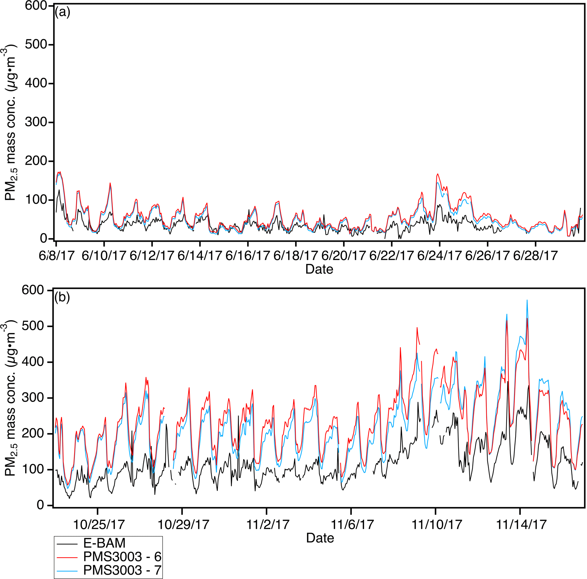
Figure 9Comparison of hourly PM2.5 mass concentrations between the E-BAM and the two uncalibrated PMS3003 sensor packages (a) from 8 to 29 June 2017 (monsoon season) and (b) from 23 October to 16 November 2017 (post-monsoon season) at IIT Kanpur.
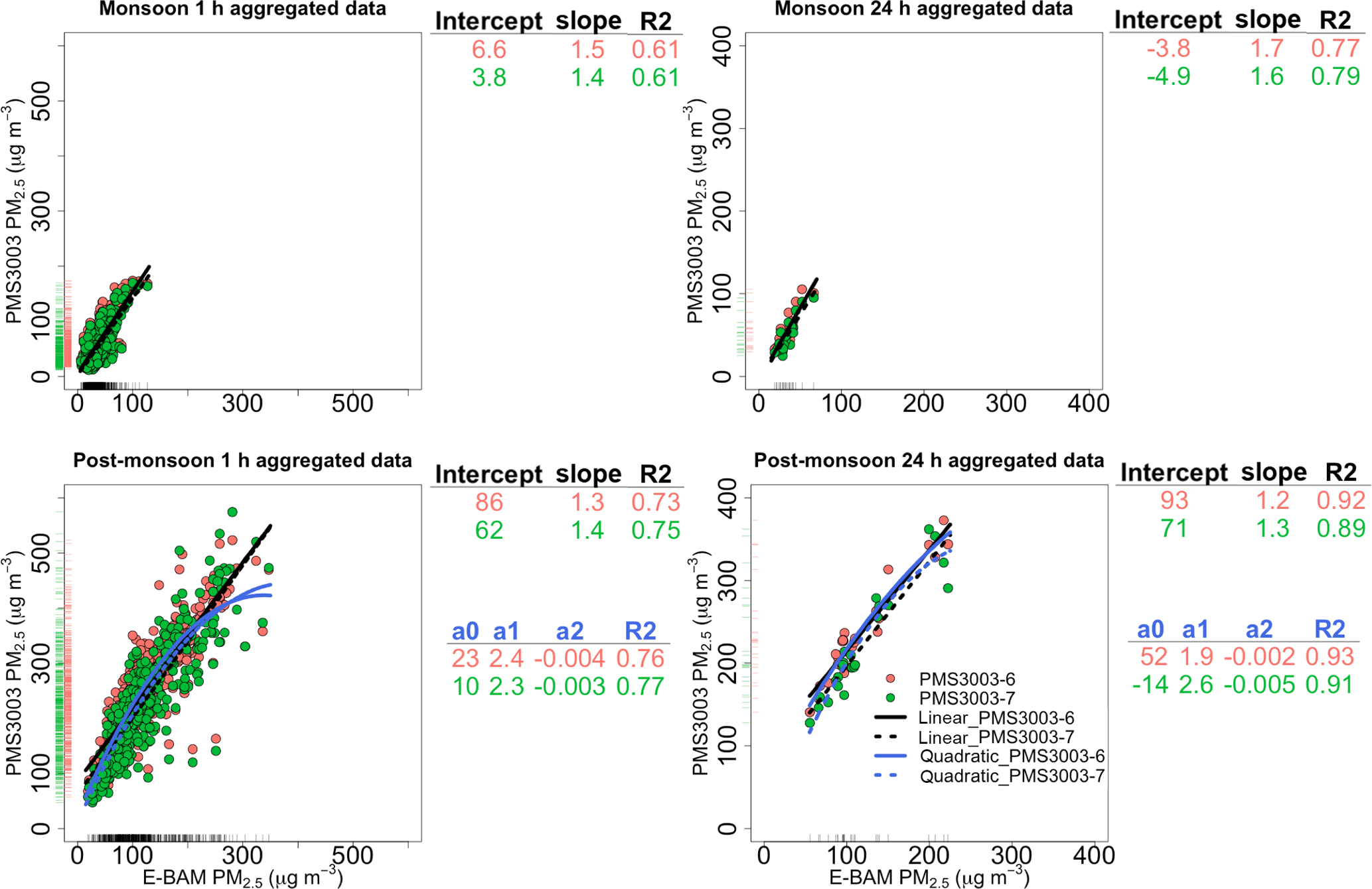
Figure 10Linear regressions between aggregated PM2.5 mass concentrations (µg m−3) of the E-BAM and the two uncalibrated PMS3003 sensors at 1 and 24 h time intervals during the monsoon season (from 8 to 29 June 2017) and the post-monsoon season (from 23 October to 16 November 2017) at IIT Kanpur (6 and 12 h results are shown in Fig. S9). The fit coefficients for the calibration models are provided. Marginal rugs were added to better visualize the distribution of data on each axis.
Despite the slight potential change, higher PMS3003–E-BAM correlations were found in the post-monsoon season than the monsoon season over all time-averaging intervals (Table 4). Figure 10 displays the 1 and 24 h average regression plots for the two uncalibrated sensors against the E-BAM during the monsoon and post-monsoon seasons. Similar to the Durham and EPA RTP field tests, different PMS3003 units had similar calibration factors over the same averaging timescales during both seasons. Comparable to the EPA RTP evaluation, the sensor units at or in the same study location or season were roughly similar in sensitivity and baseline regardless of averaging time periods (Fig. 10 and Table 4). Figure 10 also shows a distinct baseline drift of the PMS3003 sensors from the monsoon to the post-monsoon season regime. This appreciable drift in baseline agreed with the sensors being incapable of reaching the local minima of true ambient PM2.5 concentrations. This may also suggest a performance change or may be a reflection of a different calibration regime.
Table 4Summary of sensor performance characteristics for the two PMS3003 PM2.5 measurements at 1, 6, 12, and 24 h time intervals during the monsoon season (Mon, 8 to 29 June 2017) and for two different calibration methods (i.e., simple linear and quadratic equations) during the post-monsoon season (PoM, 23 October to 16 November 2017) at IIT Kanpur. The fit coefficients are provided for only the linear regression calibration models. The R2, mean of ratios, and error are performance characteristics for the calibrated PMS3003 PM2.5 measurements after the entire suite of indicated adjustments in comparison with reference values. The results are displayed in mean (range) format. Note the mean statistics were obtained by fitting the models to the PMS3003 PM2.5 measurements averaged across all the two sensor package units at each point in time.
β0: intercept. β1: coefficient for
E-BAM. β2: coefficient for temperature (T). 1 Mean of
ratios of calibrated PMS3003 to E-BAM PM2.5 concentration. 2 Defined as 1 SD
of ratios of calibrated PMS3003 to E-BAM PM2.5 concentration.
3 No attempt
was made to incorporate a temperature variable in quadratic models.
4 Temperature variable was not statistically significant at the 12 h
time resolution for the monsoon data set.
Figure 11 depicts a heat map of mean errors in calibrated PMS3003 PM2.5 measurements with respect to averaging timescales and calibration methods across varied sampling locations or seasons. Even though the EPA RTP sampling location had the lowest ambient PM2.5 level among the three study locations, it achieved the highest accuracy over each averaging time period, therefore reiterating the vital role the precision of reference instruments plays in evaluating sensor performance. For the remaining two sampling sites with an E-BAM as the reference monitor, lower errors were generally found in higher PM2.5 concentration environments. The exceptions to this rule were observed at 12 h (Kanpur post-monsoon error > monsoon error) and 24 h (Kanpur monsoon error > Duke University site error) time intervals. The occurrence of these anomalies can be explained by stronger smoothing effects than PM2.5 concentration effects over longer averaging times. Table 4 details the errors in calibrated PMS3003 PM2.5 measurements during the monsoon and post-monsoon seasons in Kanpur. The appreciably narrower reductions in mean errors from the 1 to 24 h scale during both seasons in Kanpur (monsoon: 46 % to 17 %, post-monsoon: 35 % to 11 %) compared to the reduction at the Duke University site (201 % to 15 %) underscore the inferior precision of E-BAM at low ambient PM2.5 concentrations.
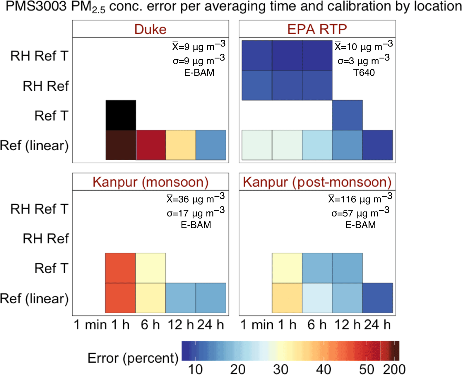
Figure 11Heat map of the mean errors of the calibrated PMS3003 PM2.5 measurements with respect to averaging timescales and calibration methods across study sites or sampling seasons. The mean and SD of the true ambient PM2.5 concentrations reported by the corresponding reference instrument (Ref) for each location or season were overlaid on the heat map. Note the errors of the 1 h E-BAM calibrated and the combination of E-BAM and temperature (T) calibrated PMS3003 PM2.5 measurements at the Duke study site were 201 % and 207 %, respectively. They are represented by dark brown and black, respectively, to improve the visual contrast in errors.
The lack of requirement for RH corrections during both testing seasons in Kanpur paralleled the outcomes of the Duke University field test. Figure S7 shows that the empirical RH correction equation fitted poorly with the widely scattered data from both monsoon (R2≤0.13) and post-monsoon seasons (R2≤0.03). We speculate that the E-BAM's low precision might be responsible for the failure to establish the impact of RH on PMS3003 responses, considering that the T640 measurements resulted in a significant RH relationship under similar conditions. We attempted to apply the empirical RH adjustment equations derived at the EPA RTP testing site to the Kanpur and Duke University data sets. However, no improvements in correlations or errors were found, indicating the RH correction function appears to be highly specific to study sites because of its great reliance on particle chemical, microphysical, and optical properties (Laulainen, 1993). The temperature variable was found to be statistically significant and therefore incorporated in the calibration models at time resolutions finer than 6 h for the Kanpur monsoon data and finer than 12 h for the post-monsoon data (Table S1). Overall, the temperature adjustments can scale the PMS3003 PM2.5 measurement errors down by no more than 7 %, with the 6 h averaged data during the post-monsoon season marking the greatest improvement (Table 4). These marginal improvements were comparable to those observed at the EPA RTP testing site (within 4 %).
3.3.3 Comparing among the methods for calibrating the Kanpur post-monsoon measurements
We observed a relatively pronounced nonlinear relationship between the raw PMS3003 and the E-BAM PM2.5 responses over the full concentration range examined during the post-monsoon season at IIT Kanpur (Fig. 10). In previous research, similar nonlinearity was ubiquitously characterized by attenuated responses towards the upper end of low-cost sensors' operation range in both field campaigns (Gao et al., 2015; Kelly et al., 2017; Johnson et al., 2018) and laboratory settings (Austin et al., 2015; Wang et al., 2015). The shape of calibration curves is dependent on varied factors such as type of low-cost sensor, range of true ambient PM2.5 concentrations, particle size, and particle composition (Wang et al., 2015). Without additional information, we are unable to parse out the exact reasons for the occurrence of this nonlinearity in our data during the Indian post-monsoon season. Nevertheless, we speculate that the comparatively high concentration range along with the prevalence of small particles encountered during the post-monsoon season might account for this nonlinearity (Kelly et al., 2017). In the present study, the PMS3003 responses were well characterized by a linear model below ∼125 µg m−3, which was close to the highest 1 h PM2.5 concentration during the monsoon season. This threshold was around 3 times greater than that reported by Kelly et al. (2017), who field-tested PMS1003 sensors under an ammonium-nitrate-dominated, moderately high PM2.5 concentration condition (1 h PM2.5 mean: up to 20 µg m−3, range: 10–70.6 µg m−3).
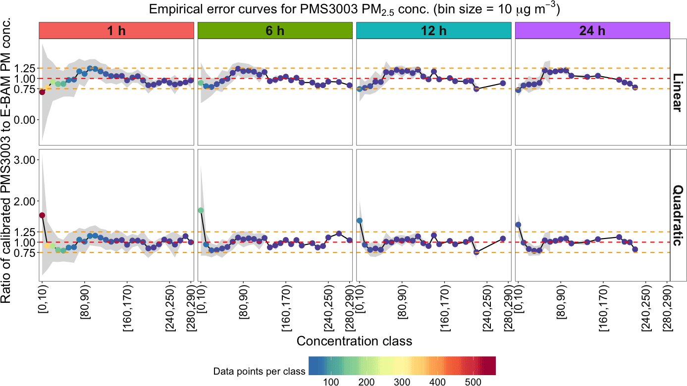
Figure 12Empirical error curves for the E-BAM calibrated Plantower PMS3003 PM2.5 measurements at 1, 6, 12, and 24 h time intervals from two different calibration methods (i.e., simple linear and quadratic equations). The curves were generated from the combination of the Duke University and IIT Kanpur data sets. The points and lines represent the means of ratios of E-BAM-calibrated PMS3003 to E-BAM PM2.5 measurements in different concentration classes, each of which spans a 10 µg m−3 interval. The shaded region represents the corresponding magnitudes of errors of PMS3003 PM2.5 measurements after the E-BAM calibration. The concentration classes are color coded by the number of data points in each class. Note the shaded region is generally absent from near the upper end of the PM2.5 ranges due to insufficient observations for the error evaluation. The red dashed line indicates a ratio of 1, while the two orange dashed lines indicate ratios of 0.75 and 1.25, respectively.
Researchers have used higher-order polynomial (Austin et al., 2015; Gao et al., 2015), penalized spline (Austin et al., 2015), and exponential functions (Kelly et al., 2017) to capture nonlinear responses of low-cost sensors. In this study, we explored the quadratic model to describe the full range response of the PMS3003 sensors during the Kanpur post-monsoon season. The quadratic model was chosen because it is straightforward to understand, interpret, disseminate, and use. The time series of the 1 and 24 h averages of the calibrated PMS3003 PM2.5 responses using the two calibration models (i.e., simple linear and quadratic models) can be found in Fig. S8. Figure S8 shows that the quadratic model might suit the post-monsoon 1 h aggregated data better than the simple linear model as the simple linear model failed to capture the local minima of the E-BAM throughout the post-monsoon period. The two models only differed little for the 24 h aggregated data. This is expected as Figs. 10 and S9 show that the strength of nonlinearity declined as the averaging times increased because longer averaging times reduced the number of relatively low-concentration observations (such as below ∼100 µg m−3). Table S2 summarizes the goodness of fit and accuracy estimates for the two model types as a function of time-averaging intervals during the post-monsoon season. Table S2 indicates that the quadratic fit appeared to have better goodness of fit and accuracy estimates for the current post-monsoon data set than the simple linear fit with both lower AIC and RMSE values at all time resolutions. Compared to the simple linear model, the quadratic model could further improve the mean accuracy of PMS3003 PM2.5 responses by up to 11 % (Table 4). Even when the nonlinearity was not strong enough to make the simple linear fit statistically different from the quadratic fit (i.e., the quadratic term a2 in the quadratic fit (Eq. 7) not significantly different from 0 with p>0.1) at 24 h integration time, the quadratic fit can still reduce the mean error and the range of RMSEs by 2 % (Table 4) and 3 µg m−3 (Table S2), respectively. This might also shed some light on the choice of calibration methods for PMS3003 PM2.5 responses in future deployments. The quadratic model should be chosen over the simple linear model as the starting point (default approach) to PMS3003 PM2.5 response calibration since the quadratic model can always be of larger benefit to the accuracy of PMS3003 measurements than the simple linear model even when the nonlinearity is weak at low ambient PM2.5 concentrations or at longer time-averaging intervals.
3.3.4 Empirical error curves for PMS3003 PM2.5 measurements with E-BAM as the reference monitor
Empirical error curves for PMS3003 PM2.5 measurements by calibration method and averaging time are presented in Fig. 12 by combining the results of all the field tests with E-BAM as the reference monitor (i.e., Duke University and IIT Kanpur data sets). These curves are useful for easy reference to the magnitude of errors for a given concentration range at a given temporal resolution. Overall, regardless of the averaging times, the largest errors were found below 20 µg m−3, particularly in the range of 0 to 10 µg m−3. Although further work is required to improve the error curves by collecting more data points, especially near the upper end of the PM2.5 distributions, we would presume calibrated PMS3003 PM2.5 responses to be relatively stable and consistent above ∼70 µg m−3 for 1 h aggregated data and above ∼50 µg m−3 for 6 to 24 h aggregated data with uncertainties roughly confined within 25 %, particularly when the quadratic calibration models are employed.
Given the broad range in PM2.5 concentrations, Fig. 12 seems to demonstrate that the quadratic calibration method performed better than their simple linear counterpart at all time intervals with steadier mean of ratio lines (remaining more constantly at 1 regardless of concentration classes) and relatively low uncertainties. The quadratic model outperformed the simple linear model, particularly over the moderately high concentration range (i.e., ∼60–140 µg m−3). Although a lesser improvement than over the moderately high concentration range, the quadratic fit still managed to slightly tighten the shaded uncertainty region over the range of ∼30–60 µg m−3, in which few differences existed between the two calibration curves. Table S3 shows that the quadratic fit had smaller AIC and RMSE values than the simple linear fit at all time intervals. Figure S10 further shows that the quadratic models fitted remarkably better than the simple linear model to the data. These observations support using the quadratic rather than the simple linear method as the general approach in calibrating PMS3003 PM2.5 responses.
This study comprised three distinct field campaigns in both an urban-influenced setting in Kanpur, India, during both monsoon (1 h averages: [PM2.5] µg m−3; RH %; temperature ∘C) and post-monsoon seasons ([PM2.5] µg m−3; RH %; temperature ∘C) and two suburban settings in Durham ([PM2.5] µg m−3; RH %; temperature ∘C) and RTP, NC, US ([PM2.5] µg m−3; RH %; temperature ∘C). The goal is to provide the adequate range of conditions to characterize how variability in ambient PM2.5 concentrations, meteorological factors (such as temperature and RH), and reference monitor types (Durham and Kanpur: E-BAM; RTP: T640 and SHARP) can affect the performance of low-cost Plantower PMS3003 sensors' PM2.5 measurements compared with reference instruments at 1 min, 1 h, 6 h, 12 h, and 24 h integration times. This information is ultimately important for identifying suitable research or citizen science applications for these sensors given their quantified capabilities.
The lower mean errors of PMS3003 sensors at the EPA RTP site (from 27 % for 1 h to 9 % for 24 h) than those at the remaining sites (Duke: from 201 % to 15 %; Kanpur monsoon: from 46 % to 17 %; Kanpur post-monsoon: from 35 % to 11 %) underscore the critical role the precision of reference instruments (T640: ±0.5 µg m−3 for 1 h; SHARP: ±2 µg m−3 for 24 h, better than the E-BAM) plays in evaluating sensor performance and the potential unfavorableness of beta-attenuation-based monitors for testing sensors at low concentrations. Nonetheless, longer averaging times (such as 24 h) typically smoothed out noisy signals and resulted in similar levels of error, indicating the feasibility of calibrating sensors using suboptimal reference analyzers as long as an appropriate averaging time is chosen. Even though the RH correction factor models might be highly location specific, it is striking to see that they were capable of explaining up to nearly 30 % of the variance in 1 min, 1 h, and 6 h aggregated sensor measurements and reducing mean errors down from ∼22 %–27 % to roughly 10 % even at the finest 1 min time resolution. Compared to the RH corrections, temperature corrections were found to be relatively small and can only scale uncertainties down by 7 % at most; however, in addition to the other corrections, this may help to achieve the highest possible accuracy level. It is important to note that the success of both RH and temperature corrections relies on the precision of reference instruments. Properly accounting for these systematic meteorology-induced influences is helpful in making high-quality PM2.5 measurements at a low cost. Additionally, we observed that PMS3003 sensors exhibited nonlinear PM2.5 responses relative to an E-BAM when ambient PM2.5 levels exceeded ∼125 µg m−3. We found that the quadratic model is more suitable than the simple linear regression model for effectively capturing this nonlinearity and can further reduce mean errors by up to 11 %. Furthermore, we demonstrated that the quadratic model should be chosen over the simple linear model as the starting point (default approach) in calibrating PMS3003 PM2.5 responses since the quadratic model can always be of larger benefit to the accuracy of PMS3003 measurements than the simple linear model even when the nonlinearity is weak at low ambient PM2.5 concentrations or at longer time-averaging intervals. The empirical error curves constructed by pooling the results of all the field tests with E-BAMs as the reference monitor were indicative of relatively stable and consistent calibrated responses above ∼70 µg m−3 for 1 h aggregated data and above ∼50 µg m−3 for 6 to 24 h aggregated data with uncertainties roughly confined within 25 %, particularly when the quadratic calibration models are employed.
Overall, we conclude that appropriate calibration models using ideal reference monitors and dynamic adjustments for meteorological parameters are an essential prerequisite for the Plantower PMS3003 sensors to achieve high accuracy and precision over a wide range in PM2.5 concentration typically encountered in the ambient monitoring. After proper calibration, the Plantower PMS3003 low-cost PM sensors are promising monitors for dense, wireless, real-time PM sensor network development in hazy urban areas such as Delhi and Mumbai, India; to complement the existing networks by better approximating the location of major PM2.5 sources (local vs. regional) and by advancing our understanding of the influence of meteorology, such as specific wind patterns, on the resulting regional PM2.5 levels in order to guide local and regional air quality management (Hagler et al., 2006).
The data are available upon request to Tongshu Zheng (tongshu.zheng@duke.edu).
The supplement related to this article is available online at: https://doi.org/10.5194/amt-11-4823-2018-supplement.
The authors declare that they have no conflict of interest.
The U.S. Environmental Protection Agency (EPA) through its Office of Research and Development participated in this research. The views expressed in this paper are those of the authors and do not necessarily reflect the views or policies of the EPA. It has been subjected to EPA Agency review and approved for publication. Mention of trade names or commercial products does not constitute endorsement or recommendation for use.
Sachchida N. Tripathi, Shilpa Shirodkar, and Ronak Sutaria are supported
under the Research Initiative for Real-time River Water and Air Quality
Monitoring program funded by the Department of Science and Technology,
Government of India and Intel Corporation, and administered by the Indo-U.S.
Science and Technology Forum. The authors would like to thank Tim Hanley at
EPA OAQPS for providing the raw 1 min data from the T640 PM mass monitors
used in the current study. The authors are also grateful to Christina Norris
at Duke University for her insightful advice and comments on the paper.
Edited by: Paolo Laj
Reviewed by: two anonymous referees
Austin, E., Novosselov, I., Seto, E., and Yost, M. G.: Laboratory evaluation of the Shinyei PPD42NS low-cost particulate matter sensor, PLoS One, 10, 1–17, https://doi.org/10.1371/journal.pone.0137789, 2015.
Bergin, M. H., Tripathi, S. N., Jai Devi, J., Gupta, T., Mckenzie, M., Rana, K. S., Shafer, M. M., Villalobos, A. M., and Schauer, J. J.: The discoloration of the Taj Mahal due to particulate carbon and dust deposition, Environ. Sci. Technol., 49, 808–812, https://doi.org/10.1021/es504005q, 2015.
Bran, S. H. and Srivastava, R.: Investigation of PM2.5 mass concentration over India using a regional climate model, Environ. Pollut., 224, 484–493, https://doi.org/10.1016/j.envpol.2017.02.030, 2017.
Breen, M. S., Long, T. C., Schultz, B. D., Williams, R. W., Richmond-Bryant, J., Breen, M., Langstaff, J. E., Devlin, R. B., Schneider, A., Burke, J. M., Batterman, S. A., and Meng, Q. Y.: Air Pollution Exposure Model for Individuals (EMI) in Health Studies: Evaluation for Ambient PM 2.5 in Central North Carolina, Environ. Sci. Technol., 49, 14184–14194, https://doi.org/10.1021/acs.est.5b02765, 2015.
Chakrabarti, B., Fine, P. M., Delfino, R., and Sioutas, C.: Performance evaluation of the active-flow personal DataRAM PM2.5 mass monitor (Thermo Anderson pDR-1200) designed for continuous personal exposure measurements, Atmos. Environ., 38, 3329–3340, https://doi.org/10.1016/j.atmosenv.2004.03.007, 2004.
Chow, J. C.: Measurement methods to determine compliance with ambient air quality standards for suspended particles, J. Air Waste Manag. Assoc., 45, 320–382, https://doi.org/10.1080/10473289.1995.10467369, 1995.
Crawley, M. J.: 9. Statistical Modelling, in: The R Book, 2nd ed., John Wiley & Sons, UK, 388–448, 2017.
Crilley, L. R., Shaw, M., Pound, R., Kramer, L. J., Price, R., Young, S., Lewis, A. C., and Pope, F. D.: Evaluation of a low-cost optical particle counter (Alphasense OPC-N2) for ambient air monitoring, Atmos. Meas. Tech., 11, 709–720, https://doi.org/10.5194/amt-11-709-2018, 2018.
Cross, E. S., Williams, L. R., Lewis, D. K., Magoon, G. R., Onasch, T. B., Kaminsky, M. L., Worsnop, D. R., and Jayne, J. T.: Use of electrochemical sensors for measurement of air pollution: correcting interference response and validating measurements, Atmos. Meas. Tech., 10, 3575–3588, https://doi.org/10.5194/amt-10-3575-2017, 2017
Day, D. E. and Malm, W. C.: Aerosol light scattering measurements as a function of relative humidity: A comparison between measurements made at three different sites, Atmos. Environ., 35, 5169–5176, https://doi.org/10.1016/S1352-2310(01)00320-X, 2001.
Gao, M., Cao, J., and Seto, E.: A distributed network of low-cost continuous reading sensors to measure spatiotemporal variations of PM2.5 in Xi'an, China, Environ. Pollut., 199, 56–65, https://doi.org/10.1016/j.envpol.2015.01.013, 2015.
Gaur, A., Tripathi, S. N., Kanawade, V. P., Tare, V., and Shukla, S. P.: Four-year measurements of trace gases (SO2, NOx, CO, and O3) at an urban location, Kanpur, in Northern India, J. Atmos. Chem., 71, 283–301, https://doi.org/10.1007/s10874-014-9295-8, 2014.
Ghosh, S., Gupta, T., Rastogi, N., Gaur, A., Misra, A., Tripathi, S. N., Paul, D., Tare, V., Prakash, O., Bhattu, D., Dwivedi, A. K., Kaul, D. S., Dalai, R., and Mishra, S. K.: Chemical characterization of summertime dust events at Kanpur: Insight into the sources and level of mixing with anthropogenic emissions, Aerosol Air Qual. Res., 14, 879–891, https://doi.org/10.4209/aaqr.2013.07.0240, 2014.
Hagler, G. S. W., Bergin, M. H., Salmon, L. G., Yu, J. Z., Wan, E. C. H., Zheng, M., Zeng, L. M., Kiang, C. S., Zhang, Y. H., Lau, A. K. H., and Schauer, J. J.: Source areas and chemical composition of fine particulate matter in the Pearl River Delta region of China, Atmos. Environ., 40, 3802–3815, https://doi.org/10.1016/j.atmosenv.2006.02.032, 2006.
Holstius, D. M., Pillarisetti, A., Smith, K. R., and Seto, E.: Field calibrations of a low-cost aerosol sensor at a regulatory monitoring site in California, Atmos. Meas. Tech., 7, 1121–1131, https://doi.org/10.5194/amt-7-1121-2014, 2014.
Jiao, W., Hagler, G., Williams, R., Sharpe, R., Brown, R., Garver, D., Judge, R., Caudill, M., Rickard, J., Davis, M., Weinstock, L., Zimmer-Dauphinee, S., and Buckley, K.: Community Air Sensor Network (CAIRSENSE) project: evaluation of low-cost sensor performance in a suburban environment in the southeastern United States, Atmos. Meas. Tech., 9, 5281–5292, https://doi.org/10.5194/amt-9-5281-2016, 2016.
Johnson, K. K., Bergin, M. H., Russell, A. G., and Hagler, G. S. W.: Field Test of Several Low-Cost Particulate Matter Sensors in High and Low Concentration Urban Environments, Aerosol Air Qual. Res., 18, 565–578, https://doi.org/10.4209/aaqr.2017.10.0418, 2018.
Kelly, K. E., Whitaker, J., Petty, A., Widmer, C., Dybwad, A., Sleeth, D., Martin, R., and Butterfield, A.: Ambient and laboratory evaluation of a low-cost particulate matter sensor, Environ. Pollut., 221, 491–500, https://doi.org/10.1016/j.envpol.2016.12.039, 2017.
Laulainen, N. S.: Summary of conclusions and recommendations from a visibility science workshop; technical basis and issues for a national assessment for visibility impairment, National Center for Atmospheric Research, Boulder, Colorado, 35 pp., available at: http://www.osti.gov/energycitations/product.biblio.jsp?osti_id=10149541 (last access: 10 January 2018), 1993.
Lewis, A. and Edwards, P.: Validate personal air-pollution sensors, Nature, 535, 29–31, 2016.
Li, Z., Li, L., Zhang, F., Li, D., Xie, Y., and Xu, H.: Comparison of aerosol properties over Beijing and Kanpur: Optical, physical properties and aerosol component composition retrieved from 12 years ground-based Sun-sky radiometer remote sensing data, J. Geophys. Res.-Atmos., 120, 1520–1535, https://doi.org/10.1002/2014JD022593, 2015.
Met One Instruments: E-BAM-9800 Operation Manual Rev L, available at: http://www.equipcoservices.com/pdf/manuals/met_one_e-bam.pdf (last access: 10 January 2018), 2008.
Mukherjee, A., Stanton, L. G., Graham, A. R., and Roberts, P. T.: Assessing the utility of low-cost particulate matter sensors over a 12-week period in the Cuyama valley of California, Sensors (Switzerland), 17, 1805, https://doi.org/10.3390/s17081805, 2017.
North Carolina Department of Environmental Quality: PM2.5 Average Values, available at: https://deq.nc.gov/about/divisions/air-quality/air-quality-data/nata-epa-national-air-toxics-assessment-for-north-carolina/data-archives-statistical-summaries/design-value-summaries/pm25-average-values (last access: 10 January 2018), 2017.
North Carolina Department of Transportation: Urban-Area Traffic Volume Maps, available at: https://xfer.services.ncdot.gov/imgdot/DOTTSUMaps/AADT_URBANS/DURHAM_URBAN/2015/Durham.pdf (last access: 10 January 2018), 2015.
Pope, C. A. and Dockery, D. W.: Health effects of fine particulate air pollution: Lines that connect, J. Air Waste Manag. Assoc., 56, 709–742, https://doi.org/10.1080/10473289.2006.10464485, 2006.
Ram, K., Sarin, M. M., and Tripathi, S. N.: A 1 year record of carbonaceous aerosols from an urban site in the Indo-Gangetic Plain: Characterization, sources, and temporal variability, J. Geophys. Res.-Atmos., 115, D24313, https://doi.org/10.1029/2010JD014188, 2010.
Shamjad, P. M., Tripathi, S. N., Pathak, R., Hallquist, M., Arola, A., and Bergin, M. H.: Contribution of Brown Carbon to Direct Radiative Forcing over the Indo-Gangetic Plain, Environ. Sci. Technol., 49, 10474–10481, https://doi.org/10.1021/acs.est.5b03368, 2015.
Sinclair, D., Countess, R. J., and Hoopes, G. S.: Effect of relative humidity on the size of atmospheric aerosol particles, Atmos. Environ., 8, 1111–1117, https://doi.org/10.1016/0004-6981(74)90045-6, 1974.
Sivaprasad, P. and Babu, C. A.: Seasonal variation and classification of aerosols over an inland station in India, Meteorol. Appl., 21, 241–248, https://doi.org/10.1002/met.1319, 2014.
Snyder, E. G., Watkins, T. H., Solomon, P. A., Thoma, E. D., Williams, R. W., Hagler, G. S. W., Shelow, D., Hindin, D. A., Kilaru, V. J., and Preuss, P. W.: The Changing Paradigm of Air Pollution Monitoring, Environ. Sci. Technol., 47, 11369–11377, https://doi.org/10.1021/es4022602, 2013.
Soneja, S., Chen, C., Tielsch, J. M., Katz, J., Zeger, S. L., Checkley, W., Curriero, F. C., and Breysse, P. N.: Humidity and gravimetric equivalency adjustments for nephelometer-based particulate matter measurements of emissions from solid biomass fuel use in cookstoves, Int. J. Environ. Res. Pu., 11, 6400–6416, https://doi.org/10.3390/ijerph110606400, 2014.
Sousan, S., Koehler, K., Hallett, L., and Peters, T. M.: Evaluation of consumer monitors to measure particulate matter, J. Aerosol Sci., 107, 123–133, https://doi.org/10.1016/j.jaerosci.2017.02.013, 2017.
South Coast Air Quality Management District (SCAQMD): Field Evaluation AirBeam PM Sensor, available at: http://www.aqmd.gov/docs/default-source/aq-spec/field-evaluations/airbeam—field-evaluation.pdf?sfvrsn=4 (last access: 10 January 2018), 2015a.
South Coast Air Quality Management District (SCAQMD): Field Evaluation AlphaSense OPC-N2 Sensor, available at: http://www.aqmd.gov/docs/default-source/aq-spec/field-evaluations/alphasense-opc-n2—field-evaluation.pdf?sfvrsn=0 (last access: 10 January 2018), 2015b.
South Coast Air Quality Management District (SCAQMD): Field Evaluation Laser Egg PM Sensor, available at: http://www.aqmd.gov/docs/default-source/aq-spec/field-evaluations/laser-egg—field-evaluation.pdf (last access: 10 January 2018), 2017a.
South Coast Air Quality Management District (SCAQMD): Field Evaluation Purple Air PM Sensor, available at: http://www.aqmd.gov/docs/default-source/aq-spec/field-evaluations/purpleair—field-evaluation.pdf (last access: 10 January 2018), 2017b.
South Coast Air Quality Management District (SCAQMD): Field Evaluation Purple Air (PA-II) PM Sensor, available at: http://www.aqmd.gov/docs/default-source/aq-spec/field-evaluations/purple-air-pa-ii—field-evaluation.pdf?sfvrsn=2 (last access: 10 January 2018), 2017c.
Teledyne Advanced Pollution Instrumentation (API): Teledyne API T640 PM Mass Monitor User Manual, available at: http://www.teledyne-api.com/prod/Downloads/T640 Manual - 08354.pdf (last access: 10 January 2018), 2016.
Thermo Fisher Scientific: Model 5030 SHARP Monitor Instruction Manual, available at: http://unitylabservices.info/content/dam/tfs/ATG/EPD/EPD Documents/Product Manuals & Specifications/Air Quality Instruments and Systems/Particulate/EPM-manual-Model 5030 SHARP.pdf (last access: 10 January 2018), 2007.
U.S. Environmental Protection Agency (U.S. EPA): Health and Environmental Effects of Particulate Matter (PM), available at: https://www.epa.gov/pm-pollution/health-and-environmental-effects-particulate-matter-pm (last access: 10 January 2018), 2016a.
U.S. Environmental Protection Agency (U.S. EPA): NAAQS Table, available at: https://www.epa.gov/criteria-air-pollutants/naaqs-table (last access: 10 January 2018), 2016b.
U.S. Environmental Protection Agency (U.S. EPA): U.S. EPA awards $750,000 for air monitoring sensors in Southern California, available at: https://19january2017snapshot.epa.gov/newsreleases/us-epa-awards-750000-air-monitoring-sensors-southern-california_.html (last access: 10 January 2018), 2016c.
U.S. Environmental Protection Agency (U.S. EPA): EPA scientists develop Federal Reference & Equivalent Methods for measuring key air pollutants, available at: https://www.epa.gov/air-research/epa-scientists-develop-federal-reference-equivalent-methods-measuring-key-air (last access: 10 January 2018), 2017.
Villalobos, A. M., Amonov, M. O., Shafer, M. M., Devi, J. J., Gupta, T., Tripathi, S. N., Rana, K. S., Mckenzie, M., Bergin, M. H., and Schauer, J. J.: Source apportionment of carbonaceous fine particulate matter (PM2.5) in two contrasting cities across the Indo–Gangetic Plain, Atmos. Pollut. Res., 6, 398–405, https://doi.org/10.5094/APR.2015.044, 2015.
Waggoner, A. P., Weiss, R. E., Ahlquist, N. C., Covert, D. S., Will, S., and Charlson, R. J.: Optical characteristics of atmospheric aerosols, Atmos. Environ., 15, 1891–1909, https://doi.org/10.1016/0004-6981(81)90224-9, 1981.
Wang, Y., Li, J., Jing, H., Zhang, Q., Jiang, J., and Biswas, P.: Laboratory Evaluation and Calibration of Three Low-Cost Particle Sensors for Particulate Matter Measurement, Aerosol Sci. Technol., 49, 1063–1077, https://doi.org/10.1080/02786826.2015.1100710, 2015.
Williams, R., Suggs, J., Rea, A., Leovic, K., Vette, A., Croghan, C., Sheldon, L., Rodes, C., Thornburg, J., Ejire, A., Herbst, M., and Sanders, W.: The Research Triangle Park particulate matter panel study: PM mass concentration relationships, Atmos. Environ., 37, 5349–5363, https://doi.org/10.1016/j.atmosenv.2003.09.019, 2003.
Williams, R., Conner, T., Clements, A., Foltescu, V., Nthusi, V., Jabbour, J., Nash, D., Rice, J., Kaufman, A., Rourk, A., and Srivastava, M.: Performance Evaluation of the United Nations Environment Programme Air Quality Monitoring Unit, EPA/600/R-17/171, available at: https://www.epa.gov/sites/production/files/2017-07/documents/un_pod_report-7-12-17.pdf (last access: 10 January 2018), 2017.
Zhang, X., Turpin, B. J., McMurry, P. H., Hering, S. V., and Stolzenburg, M. R.: Mie theory evaluation of species contributions to 1990 wintertime visibility reduction in the grand canyon, Air Waste, 44, 153–162, https://doi.org/10.1080/1073161X.1994.10467244, 1994.
Zimmerman, N., Presto, A. A., Kumar, S. P. N., Gu, J., Hauryliuk, A., Robinson, E. S., Robinson, A. L., and R. Subramanian: A machine learning calibration model using random forests to improve sensor performance for lower-cost air quality monitoring, Atmos. Meas. Tech., 11, 291–313, https://doi.org/10.5194/amt-11-291-2018, 2018.