2.1 CALIOP

Orbiting aboard the CALIPSO satellite within the A-Train constellation (Stephens et al., 2002), CALIOP is a two-wavelength (532 and 1064 nm) polarization-sensitive (at 532 nm) elastic backscatter lidar, observing the vertical distribution of aerosols and clouds in Earth's atmosphere since June 2006 (Winker et al., 2010). The 532 nm backscatter profiles measured by CALIOP are used to detect aerosol and cloud features and then retrieve corresponding particle extinction and subsequent AOTs (i.e., column-integrated extinction; Young and Vaughan, 2009) within layer boundaries determined by a multi-resolution layer detection scheme (Vaughan et al., 2009) and the assumption of a lidar ratio based upon aerosol or cloud type (Omar et al., 2005, 2009). For this study, 532 nm aerosol extinction coefficient data from the version 3 (V3) CALIPSO L2 5 km Aerosol Profile (L2_05kmAProf) product are utilized (Winker et al., 2009; hereafter, all references to CALIOP data imply the 532 nm channel/product). These aerosol profiles are reported in 5 km segments and feature a vertical resolution of 60 m below an altitude of 20.2 km above mean sea level (a.m.s.l.). Only CALIOP data collected during daytime conditions are considered for this study, so that comparison with aerosol observations from MODIS and AERONET can be accomplished.

Prior to analysis, advanced QA procedures are performed on the L2_05kmAProf product. This QA scheme is similar to that employed in Campbell et al. (2012) and Winker et al. (2013) and involves several parameters included in the L2_05kmAProf product: Extinction_Coefficient_532 (≥ 0 and ≤ 1.25 km⁻¹), Extinction_QC_532 (= 0, 1, 2, 16, or 18), CAD_Score ($\ge -$100 and $\le -$20), and Extinction_Coefficient_Uncertainty_532 (≤ 10 km⁻¹). The Integrated_Attenuated_Backscatter_532 (≤ 0.01 sr⁻¹) parameter from the L2 5 km aerosol layer (L2_05kmALay) product is also used as a QA metric. A detailed description of these QA checks is also outlined in our most recent CALIOP-based study (Toth et al., 2016). Extinction retrievals reported in the CALIOP data products that do not pass the full suite of QA tests are converted to RFVs. To limit the influence of clouds on our analysis (i.e., in order to ensure that the RFV issue is occurring due to layer detection sensitivity and not because of attenuation effects caused by cloud presence), each aerosol profile is cloud screened using the atmospheric volume description (AVD) parameter. We implement the strictest cloud screening possible, as profiles are flagged “cloudy” if any of the bins within the CALIOP column are classified as cloud.

2.2 Aqua MODIS

As an integral part of the payloads for NASA's Terra and Aqua satellites, MODIS is a 36-channel spectroradiometer with wavelengths ranging from 0.41 to 15 µm. Seven of these channels (0.47–2.13 µm) are used to retrieve aerosol optical properties such as AOT (e.g., Levy et al., 2013). MODIS L2 aerosol products are reported at a spatial resolution of 10×10 km² at nadir, with a reported over-ocean expected error of (−0.02–10 %), (+0.04 + 10 %) (Levy et al., 2013). However, uncertainties for individual retrievals may be larger (Shi et al., 2011). Also, thin cirrus contamination may exist in the MODIS aerosol products (e.g., Toth et al., 2013). In this study, the Effective_Optical_Depth_Best_Ocean (550 nm) parameter in the L2 Collection 6 (C6) Aqua MODIS aerosol product (MYD04_L2; Levy et al., 2013) is utilized. Only those retrievals flagged as “good” and “very good” are considered for analysis, as determined by the Quality_Assurance_Ocean parameter within the MYD04_L2 files.

2.3 AERONET

Developed for the purpose of furthering aerosol research and validating satellite retrievals, NASA's AERONET program is a federated worldwide system of ground-based sun photometers that collect measurements of aerosol optical and radiative properties (Holben et al., 1998). With a reported uncertainty of ±0.01–0.02 (although this estimate is low in the presence of unscreened cirrus clouds; e.g., Chew et al., 2011), AOTs are derived at several wavelengths ranging from 340 to 1640 nm. Due to the lack of retrievals at the CALIOP wavelength, AOTs at 532 nm are computed from an interpolation of those derived at the 500 and 675 nm channels using an Ångström relationship (e.g., Shi et al., 2011; Toth et al., 2013). The highest-quality V2.0 AERONET data (level 2.0) are used in this study, as these are both cloud screened and quality assured (Smirnov et al., 2000). Also, only observations from coastal/island AERONET sites are considered for comparison with over-ocean CALIOP profiles, despite the potential overestimation of CALIOP AOT in coastal regions due to the CALIPSO aerosol-typing algorithms (e.g., Kanitz et al., 2014).

3.1 Demonstrating how CALIOP backscatter distribution can render profiles of all RFVs

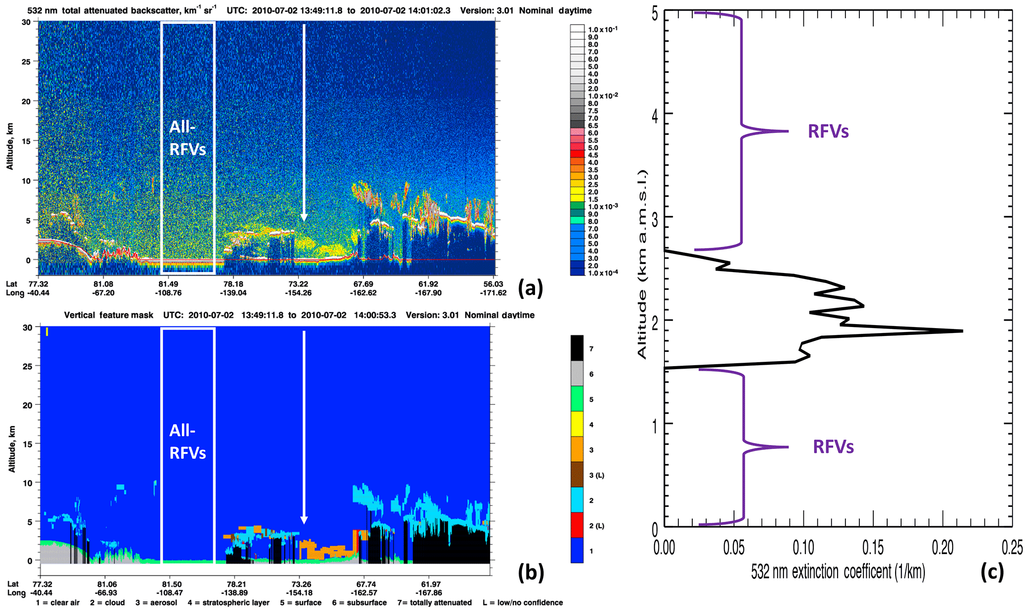
Figure 1For data collected during the daytime on 2 July 2010 over the Arctic, browse image curtain plots of CALIPSO (a) 532 nm total attenuated backscatter (km⁻¹ sr⁻¹) and (b) corresponding vertical feature mask (VFM). The white box represents an example segment of the granule for which range bins in the associated level 2 (L2) aerosol extinction coefficient profile are all retrieval fill values (RFVs), as the VFM classified these bins as either surface (green) or clear-air (blue) features. The white arrow indicates a column in which some aerosol has been detected (orange), and the resultant L2 aerosol extinction profile for this column is shown in (c).

Download

To demonstrate the nature of the RFV problem, Fig. 1 shows an example of cloud-free all-RFV CALIOP profiles embedded within curtain plots of total attenuated backscatter (TAB; Fig. 1a) and a matching vertical feature mask (VFM; Fig. 1b). Both plots were obtained from the CALIPSO Lidar Browse Images website (https://www-calipso.larc.nasa.gov/products/lidar/browse_images/production/), and the data were collected from CALIOP during the daytime on 2 July 2010 over the Arctic. The VFM shows that the range bins within the white box are classified as either surface or clear air features, and thus the corresponding L2 aerosol extinction coefficient profiles (not shown) are all-RFVs (i.e., the AOT = 0 scenario).

However, even under pristine conditions, aerosol particles are still present in the atmosphere. For example, the baseline maritime AOT is estimated to be 0.06 ± 0.01 (Kaufman et al., 2005; Smirnov et al., 2011). Thus, aerosol particles are likely present and yet undetected for the all-RFV cases shown in Fig. 1. Similar issues can also exist for profiles for which some aerosol is detected. This scenario is represented by the white arrow in the TAB and VFM plots, and the associated L2 aerosol extinction coefficient profile is depicted in Fig. 1c. An aerosol layer is evident from about 1.5 to 2.5 km a.m.s.l., leaving the remainder of the column as RFVs.

To further demonstrate the RFV phenomenon in the CALIOP data set, we next examine differences in TAB found in profiles for which all-RFVs were reported and those for which some extinction was retrieved. The CALIPSO Lidar level 1.5 data product (L1.5) is specifically leveraged for this task, as TAB for the all-RFVs class of data is not included in L2 data sets. The L1.5 product is a merging of the L1 and L2 products, cloud cleared, screened for nonaerosol features (e.g., surface, subsurface, totally attenuated, invalid), and available at 20 km (horizontal) and 60 m (vertical) resolutions (Vaughan et al., 2011). One month (February 2008) of daytime L1.5 TAB profiles over all global oceans were collocated with CALIOP AOTs derived from the L2_05kmAProf product. The data were limited to only those L1.5 averages that contain either four contiguous 5 km L2 all-RFV profiles or, conversely, four contiguous profiles for which extinction was retrieved in each. The selected TAB profiles were then averaged to a 20 km resolution for each altitude range (i.e., to obtain over global ocean mean TAB profiles).

The results of this analysis are shown in Fig. 2. Profiles of mean TAB over global oceans for February 2008 are shown in Fig. 2a; blue lines show all-RFV profiles and red lines show those for which some extinction was retrieved (i.e., non-all-RFVs). For most of the troposphere, little difference is observed between the two profiles (i.e., “clear sky” in the aggregate). However, the profiles begin to deviate below 3 km a.m.s.l., as larger TAB are found for the extinction-retrieved sample (peak TAB is ∼ 0.0031 km⁻¹ sr⁻¹) compared to those profiles consisting of all-RFVs (peak TAB value is ∼ 0.0017 km⁻¹ sr⁻¹). An additional analysis was conducted (not shown) using data over the Pacific Ocean to check for influences of geographic sampling (i.e., aerosol distribution) on the mean TAB profiles. Both the all-RFV and non-all-RFV mean TAB profiles increase at similar magnitudes after implementing this restriction, thus resulting in only a minor difference between the profiles.

Figure 2c shows a second pair of mean TAB profiles but now restricted to only those L2 CALIOP profiles collocated with MODIS AOTs between 0.03 and 0.07 (i.e., arbitrarily selected for low aerosol-loading scenarios). The collocation method applied here is the same as the one used by Toth et al. (2013), in which the midpoint of a 10×10 km² (at nadir) over-ocean MODIS AOT pixel is required to be within 8 km of the temporal midpoint of a 5 km L2 CALIOP aerosol profile. Observations outside this range are not considered. Whereas below, the modal MODIS AOT for passive retrievals collocated with all-RFV CALIOP profiles is about 0.05, this restriction (i.e., 0.03–0.07 MODIS AOTs) is meant to investigate a more nuanced question. The presence of all-RFV profiles is the result of several processes that can work either independently or in tandem. The dominant cause is, as described above, detection failure. RFVs also occur when the cloud–aerosol discrimination algorithm mistakenly classifies an aerosol layer as a cloud, and again when the extinction coefficients retrieved for a detected aerosol layer fail any of the QA metrics (e.g., an out-of-range extinction QC flag). This restriction is meant to limit the influence of layer misclassifications and occasional QA failures, and in particular, relatively high AOT cases in which unusually high TAB could influence the mean profile. Including such samples would degrade the accuracy of the TAB noise-floor estimate that we will use in subsequent analyses described in Sect. 3.5. Relatively speaking, though, the profiles in Fig. 2c are fairly similar to those of Fig. 2a. However, the relative deviation between the two samples now occurs below 2 km a.m.s.l., and the peak value of TAB for non-all-RFVs lowers to around 0.0025 km⁻¹ sr⁻¹ (illustrating the effect of the MODIS AOT restriction). Also, for context, we include corresponding profiles of attenuated scattering ratio (TAB/molecular attenuated backscatter) for both analyses in Fig. 2b and d.

The initial point of this comparison is that the mean TAB for all-RFV profiles is, as expected, lower than in those profiles for which extinction is retrieved above and within the planetary boundary layer. Thus, the figures represent a simple conceptual model of how profiles consisting of all-RFV cases arise with respect to diffuse aerosol backscatter structure and inherently lower signal-to-noise ratios (SNRs). While there are several possible strategies for mitigating this issue for future global satellite lidar missions (discussed in the concluding remarks), the goal for this initial part of the study is to simply depict how the situation is manifested in the base backscatter product measured by the sensor.

3.2 Frequency of occurrence for L2 CALIOP all-RFV aerosol profiles

The next step of the analysis is to determine the frequency of occurrence of all-RFV profiles in the daytime CALIOP L2_05kmAProf archive. As these data will be collocated with both MODIS and AERONET data for subsequent analysis, no nighttime data are considered here. Table 1 summarizes the statistics of this analysis. For the 2010–2011 period, all-RFV profiles make up about 71 % (66 %) of all daytime CALIOP L2_05kmAProf profiles globally (global oceans-only). However, these statistics include those profiles for which the CALIOP signal was totally attenuated (e.g., by an opaque cloud layer), thus inhibiting aerosol detection near the surface. For context, the 2010–2011 occurrence frequencies of CALIOP that do not detect the surface are 39.9 % (46.1 %) globally (global oceans-only). Roughly 30 % of the full archive corresponds to cloud-free conditions (again, as described in Sect. 2.1, “cloud-free” refers to the implementation of the strictest CALIOP cloud screening possible, where no clouds are classified in the entire profile). Approximately 45 % of all cloud-free profiles, and 25 % of cloud-free over-ocean profiles, are also all-RFV profiles (∼ 15 and 8 %, respectively, in absolute terms). The over-ocean sample is considered below, given the relatively higher fidelity expected in the collocated MODIS AOT data (e.g., Levy et al., 2013).

Table 1Statistical summary of the results for this study for the 2007–2008 and 2010–2011 periods, both globally and for global oceans only. The values in parentheses represent the percentages of each category relative to the entire CALIOP aerosol profile archive for each respective period.

Download Print Version | Download XLSX

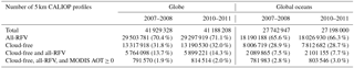
We note that due to the primary CALIOP laser failing in 2009, Table 1 also includes results from a 2-year period (2007–2008) before the laser switch to examine any differences in the statistics of the RFV issue between the two lasers. The global frequency of occurrence of all-RFV profiles is consistent for both time periods (i.e., 70.4 % for 2007–2008 and 71.1 % for 2010–2011), and thus the remainder of this paper focuses on the 2010–2011 analysis alone. We find no evidence to suggest that laser performance exhibits any significant influence on the occurrence of per-range bin RFVs and all-RFV profiles within the L2 archive.

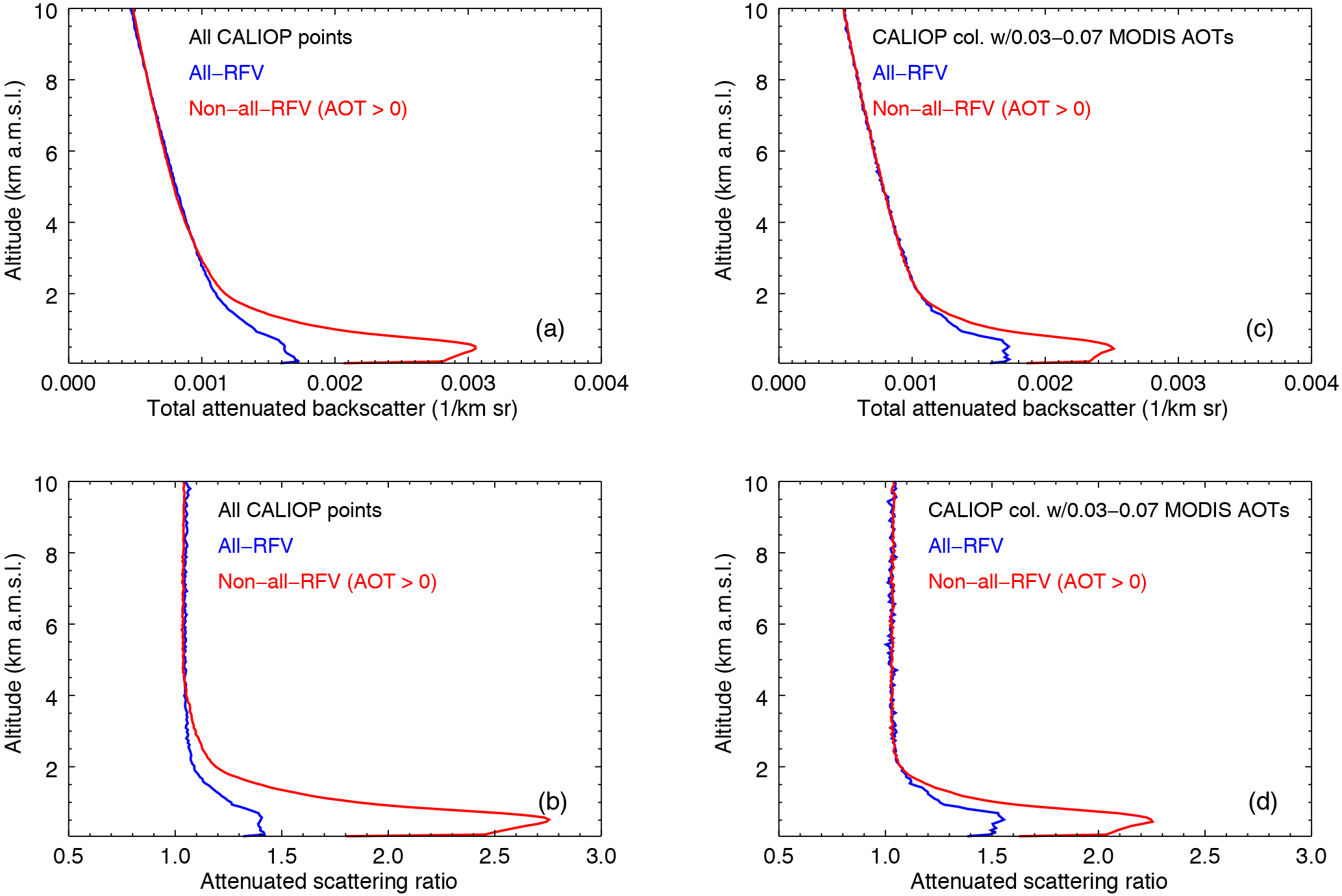
Figure 2For February 2008, mean profiles of (a, c) level 1.5 total attenuated backscatter (TAB) and (b, d) attenuated scattering ratio (TAB/molecular attenuated backscatter) over global oceans, corresponding to level 2 all-RFV (in blue) and non-all-RFV (AOT > 0; in red) profiles. The left column is from an analysis of all cloud-free CALIOP points over global oceans and the right column represents only those collocated with MODIS AOTs between 0.03 and 0.07.

Download

The spatial distribution of daytime over-ocean cloud-free all-RFV profiles is shown in Fig. 3. The percentage of cloud-free CALIOP all-RFV aerosol profiles relative to all cloud-free CALIOP aerosol profiles is computed and presented on a 2^∘ × 5^∘ latitude–longitude grid (Fig. 3a). Here we again restrict the analysis to cloud-free scenes to avoid ambiguities in RFV occurrence that are introduced by the presence of clouds. Regions with the largest occurrence frequencies of all-RFV profiles (> 75 %) include the high latitudes of both the northern and southern hemispheres (NH and SH, respectively). In fact, over snow surfaces, over 80 % of CALIOP aerosol profiles are all-RFVs. Over permanent ice (e.g., Greenland), ∼ 99 % are all-RFVs. In contrast, the tropics exhibit the lowest all-RFV profile occurrence frequencies (< 25 %). The CALIOP archive contains a significant fraction of all-RFV profiles in polar regions, which is an important result with many ramifications for NASA Earth Observing System science. It is likely that all-RFVs correlate with both low aerosol-loading scenarios and high albedo surfaces (e.g., snow and sea ice).

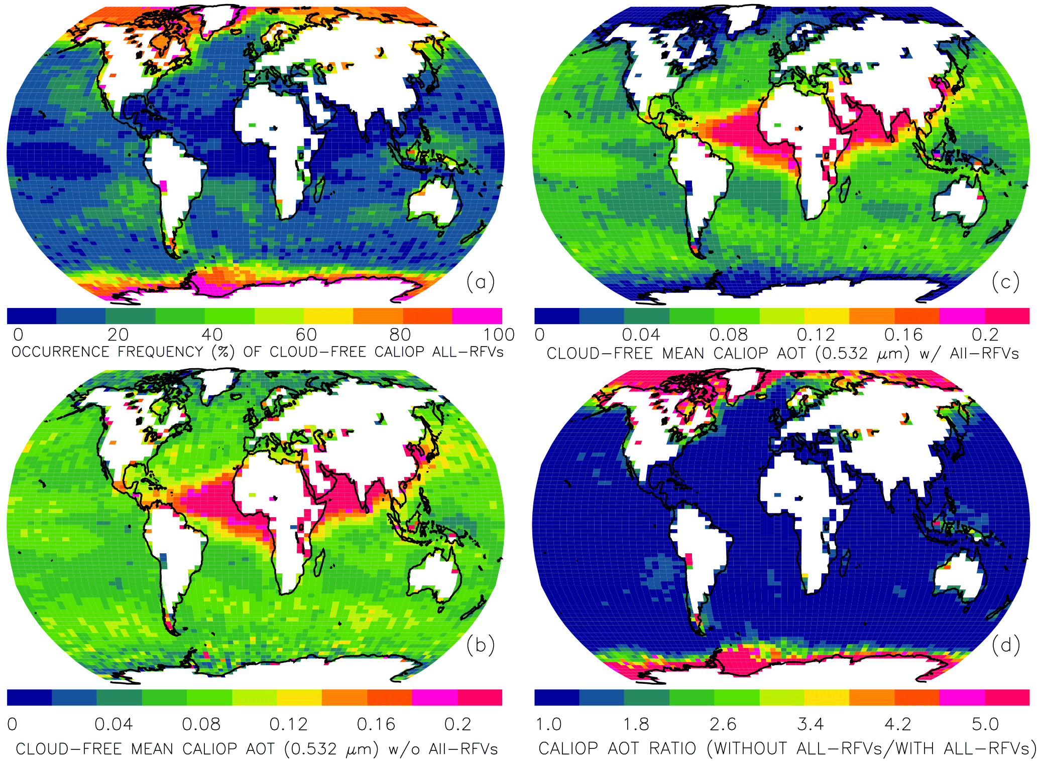
Figure 3For 2010–2011, (a) the frequency of occurrence (%) of cloud-free CALIOP profiles at 2^∘ × 5^∘ latitude–longitude grid spacing. Also shown are the corresponding cloud-free mean CALIOP column AOTs (b) without and (c) with all-RFV profiles, and (d) the ratio of (b) to (c).

Download

Figure 3 also includes the spatial distribution of mean cloud-free CALIOP-derived AOT (2^∘ × 5^∘ latitude–longitude resolution) without (Fig. 3b) and with (Fig. 3c) all-RFV profiles, demonstrating the quantitative impact of adding all-RFV AOT = 0 profiles to the relative analysis. As mentioned above, both approaches have been implemented in past studies. Comparison of the plots reveals that including the all-RFV profiles in the average naturally lowers the mean AOT. To determine the areas for which mean AOTs are most impacted by all-RFVs, the ratio of mean AOT without and with all-RFV profiles (i.e., the ratio of Fig. 3b to c) is shown in Fig. 3d. Little change in mean AOT is found for most of the oceans, with the exception of the high latitudes of each hemisphere. Overall, global ocean cloud-free mean AOT values of ∼ 0.09 and ∼ 0.07 are found, without and with all-RFV profiles, respectively. Such a decrease in mean AOT is expected, as 27 % of CALIOP L2 over-ocean cloud-free aerosol profiles are all-RFVs. Also, regions with the largest all-RFV occurrence frequencies (i.e., high latitudes of both the NH and SH) correspond to a greater lowering of mean AOT, compared with those regions (i.e., the tropics) where small all-RFV occurrence frequencies dominate.

3.3 Collocation of MODIS AOT for over-ocean CALIOP all-RFV cases

By collocating MODIS over-ocean AOT retrievals with CALIOP all-RFV profiles, we can estimate the distribution of AOT when algorithm detection/retrieval performance has been compromised. After collocation was performed (as described in Sect. 3.1), the number of all cloud-free CALIOP all-RFV profiles were binned by MODIS AOT in 0.01 increments (as depicted in Fig. 4), and separated into three latitude bands: the NH midlatitudes (30 to 60^∘ N; Fig. 4a), the tropics (−30 to 30^∘ N; Fig. 4b), and the SH midlatitudes (−60 to −30^∘ N; Fig. 4c) where coincident data densities are reasonably sufficient. For example, see Fig. 5a for numbers of valid MODIS over-ocean AOT data points available for collocation at 2^∘ × 5^∘ latitude–longitude, based on “good” or “very good” over-ocean L2 MODIS AOT retrievals, relative to all corresponding retrievals. For context, Fig. 5b shows the associated spatial distribution of mean L2 MODIS AOT. We note that this includes only those MODIS points collocated with CALIOP, and thus the AOT distributions shown in Fig. 5b are likely different from distributions derived using the full MODIS data record (e.g., Levy et al., 2013). We also note, for the reference of the reader, that histograms of C6 MODIS AOT (not collocated with CALIOP) are provided in Levy et al. (2013).

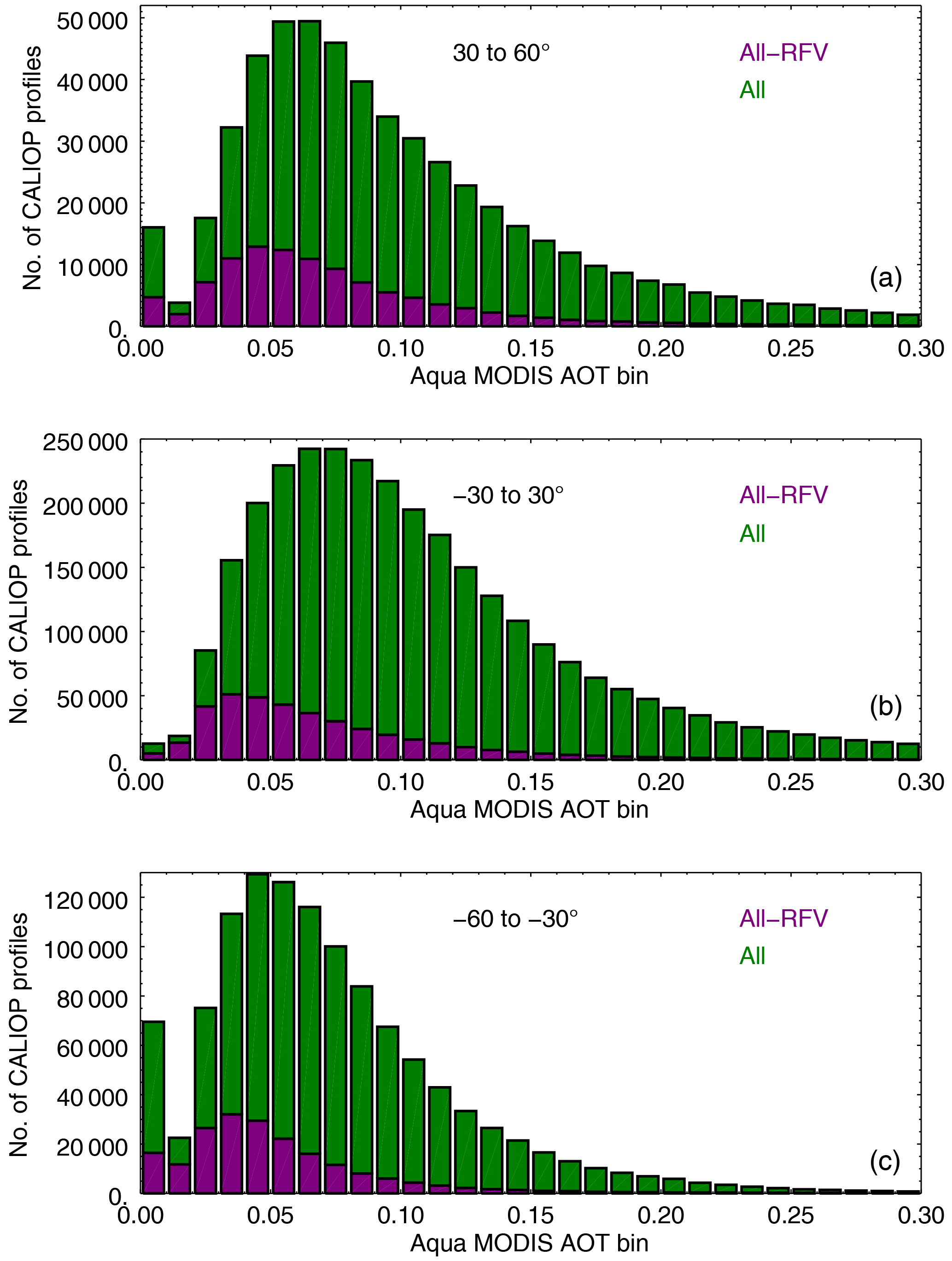
Figure 4For 2010–2011, histograms of all over-ocean cloud-free CALIOP profiles (in green) and all-RFV profiles (in purple) as a function of collocated Aqua MODIS AOT (0.01 bins), for (a) 30 to 60^∘ N, (b) −30 to 30^∘ N, and (c) −60 to −30^∘ N.

Download

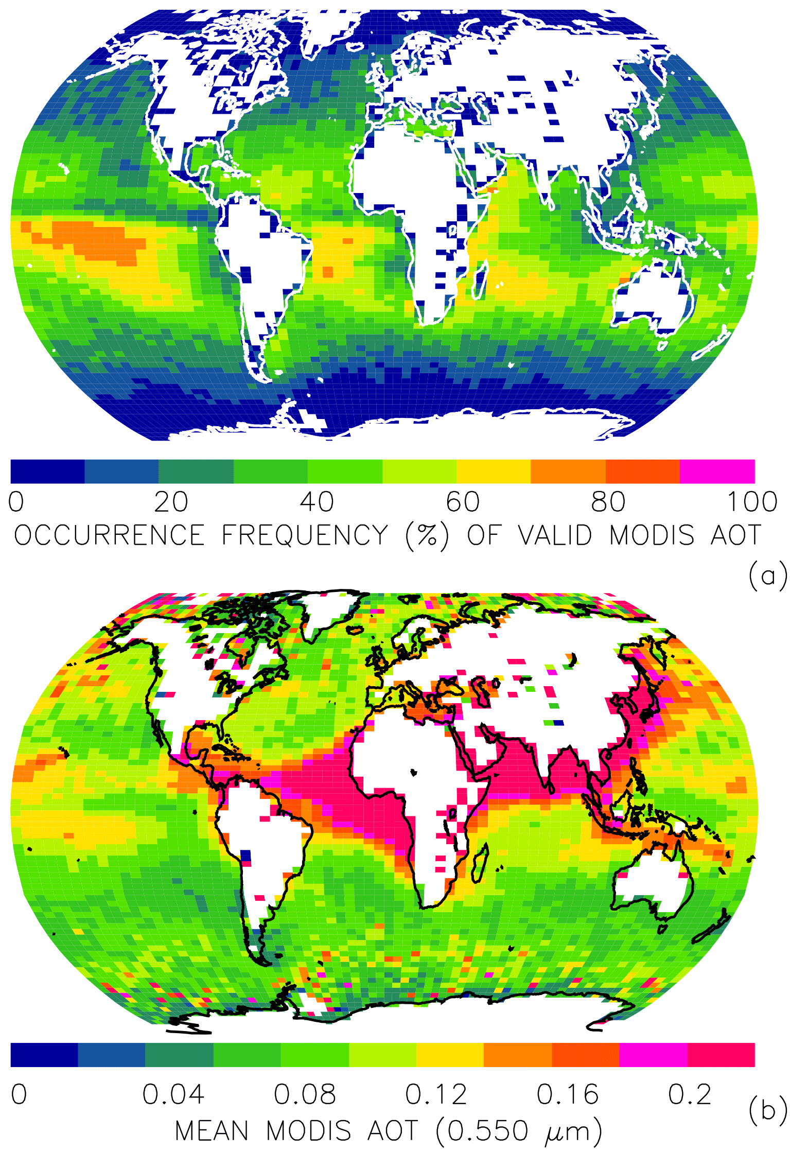
Figure 5For 2010–2011, (a) frequency of occurrence (%) of valid (“good” or “very good”) over-ocean level 2 (L2) MODIS AOT retrievals, relative to all over-ocean L2 MODIS AOT retrievals, for every 2^∘ × 5^∘ latitude–longitude grid box. Also shown is (b) the corresponding spatial distribution of mean L2 MODIS AOT for the same time period. This analysis includes only those MODIS points collocated with CALIOP.

Download

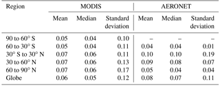
Modal values of MODIS AOT for all-RFV profiles are found between 0.03 and 0.04, with the exception of the 30 to 60^∘ N band for which the greatest number of all-RFV profiles coincide with MODIS AOTs between 0.04 and 0.05. Thus, the primary mode of CALIOP RFV profiles is 0.03–0.05 from the perspective of MODIS. Corresponding mean and median MODIS AOTs for collocated CALIOP all-RFV profiles are presented in Table 2, with a mean value of 0.07 for the tropics and NH midlatitudes and 0.05 for the SH midlatitudes band (global mean of 0.06). Median AOTs are similar, though slightly lower, with a global median of 0.05, reflecting the impact of the tail toward higher AOT in the sample distributions. We expect several modes of algorithm response contributing to these distributions, which are borne out in the CALIOP data: layer detection failures due to sensitivity limits, random noise in the attenuated backscatter measurement, and extinction retrieval failures.

Table 2Mean, median, and standard deviation of AOTs derived from Aqua MODIS (2010–2011) and AERONET (2007–2008; 2010–2011), both independently collocated with CALIOP all-RFV profiles.

Download Print Version | Download XLSX

While a similar distribution is exhibited for each region, the number of total observations for the tropics is much greater than that of the other two regions. Thus, the results of Fig. 4b are more robust, which is primarily due to MODIS AOT data availability and collocation (Fig. 5a). Total MODIS occurrence frequencies are greatest in the tropics (generally > 50 %) and decrease poleward. The midlatitude regions exhibit occurrence frequencies less than 25 %, with near-zero frequencies observed in the high latitudes of the NH and SH. We note that the low number of valid MODIS AOT retrievals in the high northern and southern latitudes, due at least partly to sea ice extent in these regions, presents a limitation for our study. That is, the areas for which all-RFV profiles occur most frequently (Fig. 3a) are the same areas with the fewest numbers of valid MODIS AOT retrievals. Note that in these regions, even for valid MODIS AOT retrievals, biases due to subpixel sea ice contamination may still exist.

All-RFV profile occurrence frequencies are computed as a function of MODIS AOT in order to quantify the amount of CALIOP-derived AOT underestimation at a given MODIS-based AOT. This underestimation (expressed as a percentage) was achieved by division of corresponding data counts in Fig. 4 and is shown in line plots in Fig. 6. The same regional sorting and MODIS AOT binning procedures from Fig. 4 are applied. A similar distribution is found for all three latitude bands, with the 0.01–0.02 MODIS AOT bin exhibiting the largest underestimation percentage, which gradually lowers toward higher MODIS AOT. CALIOP all-RFV underestimation near 50 % is found for the NH and SH midlatitude regions (the red and black curves, respectively, of Fig. 6), respectively), for MODIS AOTs between 0.01 to 0.02, and this value increases to about 70 % for the tropics (the blue curve of Fig. 6). This implies that 70 % of all cloud-free CALIOP aerosol profiles in this MODIS AOT range are underestimated (i.e., CALIOP reports cloud-free all-RFV profiles 70 % of the time for MODIS AOTs between 0.01 and 0.02).

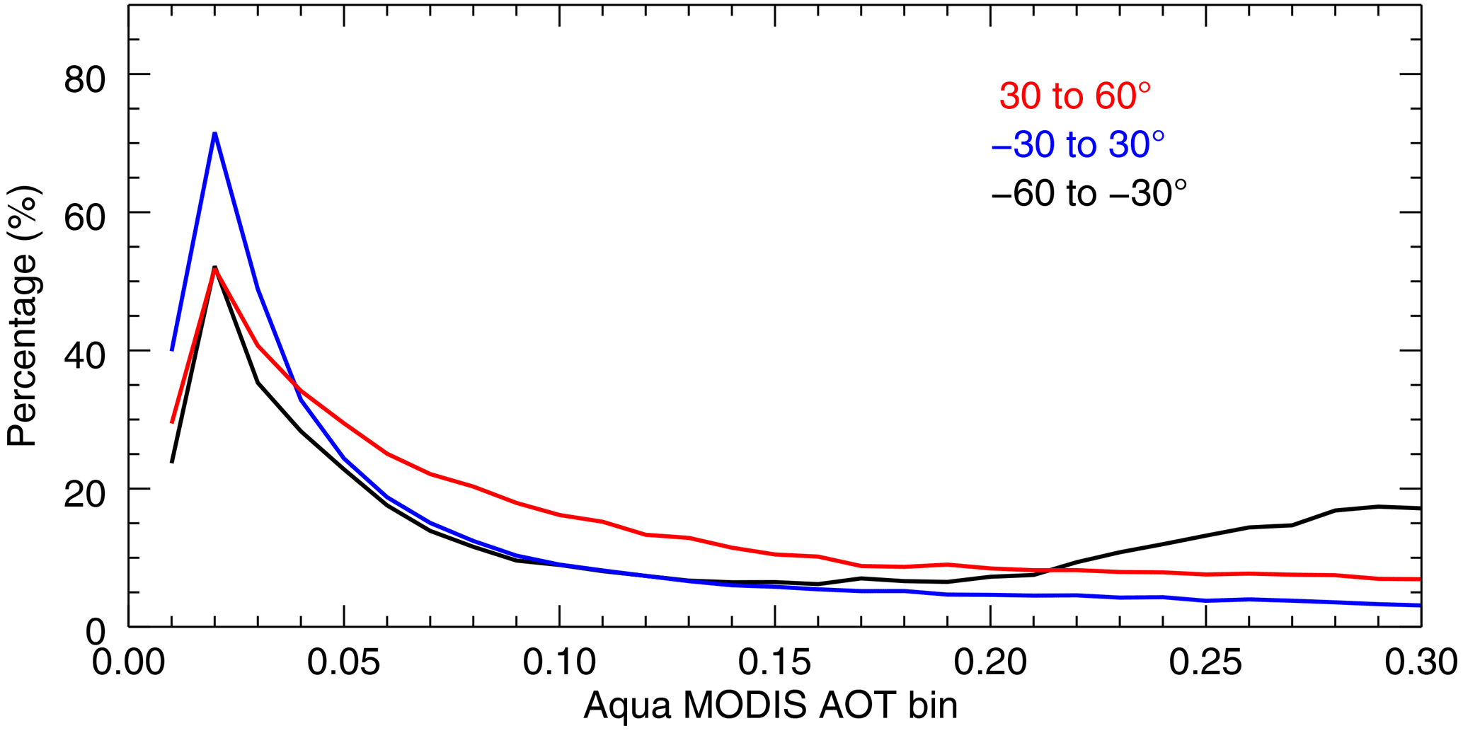
Figure 62010–2011 frequency of occurrence (%) of over-ocean cloud-free CALIOP all-RFV profiles, relative to all cloud-free CALIOP profiles, as a function of collocated Aqua MODIS AOT (0.01 bins), for 30 to 60^∘ N (in red), −30 to 30^∘ N (in blue), and −60 to −30^∘ N (in black).

Download

While the distribution for the tropics is considered most robust, due to MODIS AOT availability in this region, it is important to note that increasingly lower AOTs (i.e., below ∼ 0.03) are within the uncertainty range of MODIS AOT retrievals, and thus these results should be interpreted within the context of this caveat. Also, the relatively low underestimation percentages corresponding to MODIS AOTs less than 0.02 are believed to be an error, likely resulting from an artifact in the MODIS AOT retrievals/products.

3.4 Collocation of CALIOP all-RFV profiles with AERONET

AERONET data are considered the benchmark for satellite AOT retrievals (Holben et al., 1998). Thus, similarly to the over-ocean MODIS analysis above, CALIOP AOT and all-RFV profiles are examined using collocated AOTs derived from measurements collected at coastal and island AERONET sites. Ninety-three sites are used, the locations of which are depicted globally in Fig. 7. Similarly to Sect. 3.3, CALIOP L2_05kmAProf data are spatially (within 0.4^∘ latitude–longitude) and temporally (within 30 min) collocated with level 2.0 AERONET data. Note that we include all 4 years (2007–2008 and 2010–2011) for this analysis, as there are far fewer AERONET data points available in contrast to MODIS (e.g., Omar et al., 2013).

Figure 7Map of the 93 coastal/island AERONET sites with level 2.0 data for the 2007–2008 and 2010–2011 periods, used for collocation with over-ocean CALIOP aerosol observations.

Download

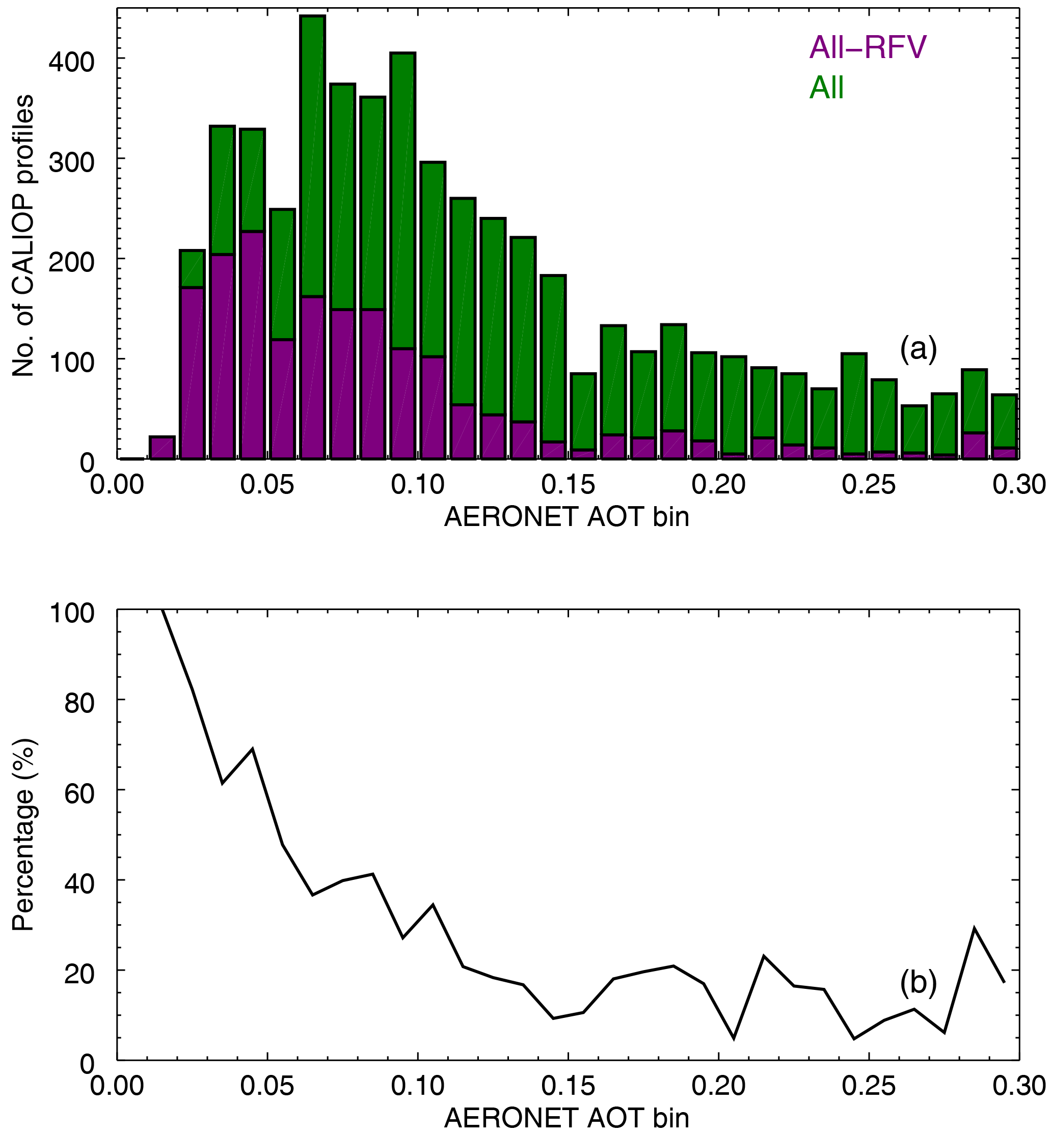
Figure 8For the 2007–2008 and 2010–2011 periods: (a) histograms of all cloud-free CALIOP profiles (in green) and all-RFV profiles (in purple), and (b) corresponding frequency of occurrence (%) of cloud-free CALIOP all-RFV profiles, relative to all cloud-free CALIOP profiles, both as a function of collocated coastal/island AERONET AOT (0.01 bins).

Download

Figure 8 summarizes the results of the CALIOP–AERONET collocation. In a similar manner to Fig. 4, Fig. 8a is a histogram of the number of cloud-free CALIOP aerosol profiles (all-RFV profiles and all available) for each 0.01 AERONET AOT bin. The overall distribution observed here is comparable to that from MODIS (Fig. 4), but noticeably noisier due to the limited AERONET data sample size. However, peak counts of all-RFV profiles occur for AERONET AOTs between 0.04 and 0.05, which is roughly consistent with the MODIS comparisons. The corresponding mean AERONET AOTs of collocated CALIOP all-RFV profiles are generally higher than those found from MODIS, with values of 0.1 and 0.09 for the tropics and NH midlatitudes, respectively (Table 2), and a global mean (median) value of 0.08 (0.07). We note that this analysis may be influenced by residual cloud contamination of subvisible cirrus in the AERONET data set (e.g., Chew et al., 2011; Huang et al., 2012). We note that histograms of sun-photometer-derived AOT from Maritime Aerosol Network (MAN) observations (i.e., over-ocean component of AERONET; not collocated with CALIOP data) are shown in Smirnov et al. (2011).

Figure 8b shows all-RFV profile occurrence frequencies as a function of AERONET AOT, computed by dividing the respective counts in Fig. 8a. Again, a noisier overall distribution is found compared with the line plots of Fig. 6. As expected, the 0.01–0.02 bin exhibits the largest underestimation percentage. However, while this value is 70 % for the MODIS analysis (the blue curve of Fig. 6), it increases to 100 % for AERONET, and we again conclude that an artifact is likely present in the MODIS retrievals for very low aerosol-loading cases. While the sample size is small, in the 4-year data set examined in this study, whenever AERONET measured an AOT lower than 0.02, the collocated CALIOP aerosol profiles contained only RFVs.

3.5 Reconciling CALIOP AOT underestimation

In this part of the study, we describe a proof-of-concept analysis that uses 1 month of data with the same spatiotemporal domain and conditions introduced in Sect. 3.1 to estimate the nominal underestimation of CALIOP AOT due to RFVs in otherwise high-fidelity L2 retrievals (i.e., those for which extinction is derived and the profile passes all QA/QC tests). This is achieved by retrieving extinction profiles from the mean global TAB profiles previously constructed from all-RFV profiles (i.e., as presented in Fig. 2). Characterizing these profiles, including those derived for all corresponding/collocated MODIS AOT (Fig. 2a, with an average MODIS AOT of 0.067) and MODIS AOT between 0.03 and 0.07 (Fig. 2c, with an average MODIS AOT of 0.045) to suppress the influence of random algorithm failure events at relatively high AOT, as TAB “noise floors”, we then replace RFV bins with corresponding extinction and calculate column-integrated AOT. The premise here assumes that the distribution of aerosol depicted in the TAB noise floors is globally constant. This is highly uncertain, and we strongly caution that the purpose is to provide an initial demonstration of a practical way to correct RFVs in the CALIOP archive.

The aerosol extinction profiles for all-RFVs are derived in two steps. First, using an assumed lidar ratio of 29 sr (standard deviation of 10 sr; derived from constrained lidar ratios over ocean and represents background aerosols for the entire atmospheric column; Kim et al., 2017), an unconstrained extinction solution is generated from 20 km to the top of the surface-attached layer (3.5 km). In this step, the molecular and aerosol attenuation in the measured backscatter is accounted for at each range bin (from a top-down approach) by taking into account the overlying molecular and aerosol loading. The aerosol backscatter is then calculated by subtracting the unattenuated molecular backscatter from the newly derived aerosol-and-molecular-attenuation-corrected backscatter, from which the aerosol extinction is derived by multiplication of the lidar ratio. The top of the surface-attached layer is determined by inspection of the ratio between the measured backscatter and the modeled molecular attenuated backscatter, as provided in the CALIPSO L1.5 product. Integrating this extinction profile provides an estimate of the AOT overlying the surface-attached layer (AOT_upper). The derived AOT_upper values are ∼ 0.015 and ∼ 0.01 for the total all-RFV sample and AOT-limited sample, respectively. These values are not surprising, as they are in agreement with AERONET measurements obtained at the Mauna Loa site (elevation of ∼ 3.5 km a.m.s.l.; Alfaro-Contreras et al., 2016).

Next, a constrained extinction solution and optimized estimate of the lidar ratio are generated from 3.5 km to the surface using the AOT of this layer (i.e., column AOT – AOT_upper). This step is similar to the abovementioned approach, except now an iterative process is implemented to derive a lidar ratio for the layer. Resulting surface-attached layer lidar ratios are 43 and 30 sr for the first and second case, respectively, with the latter value comparing reasonably well with the coastal marine lidar ratio of ∼ 28 sr derived from AERONET analyses (Sayer et al., 2012). However, the lidar ratio solved for the all-RFV sample case is higher than that typical of marine aerosols (i.e., ∼ 26 sr; Dawson et al., 2015), which may be a result of uncertainties in both MODIS and CALIOP data sets. For example, the uncertainty of the lower end of MODIS AOT retrievals is on the order of −0.02–0.04 (Levy et al., 2013). These lidar ratios are also likely to have high biases due to biases in the daytime CALIOP V3 calibration scheme: the V3 daytime calibration coefficients are typically 10 % to as much as 30 % higher than their V4 counterparts, depending on location and season (Getzewich et al., 2016). Additionally, some all-RFV profiles may include nonmarine aerosols, which would further contribute to the high biases in the retrieved lidar ratios.

Despite these caveats, the resultant all-RFV extinction profiles are shown in Fig. 9, with values peaking near the surface and decreasing exponentially with height. These are thus considered the corresponding/approximated CALIOP extinction-based noise floors. Next, for those cloud-free, over-ocean, L2_05kmAProf CALIOP profiles from the same month (February 2008), RFV bins for profiles for which some measure of extinction has been observed and passed QA/QC were replaced with the corresponding extinction noise-floor values solved for the two TAB samples. Profiles were then reintegrated to yield RFV-corrected AOTs.

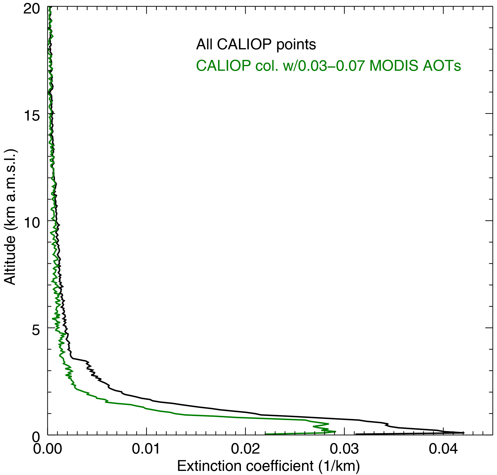
Figure 9For February 2008 over cloud-free global oceans: the all-RFV aerosol extinction coefficient profiles derived from the inversion algorithm. The black curve represents all cloud-free CALIOP profiles over global oceans, while the green curve is from an analysis restricted to only those CALIOP points collocated with MODIS AOTs between 0.03 and 0.07.

Download

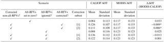
The results of this exercise are summarized in Table 3. The first result, representing the inclusion of all-RFV profiles as is within bulk global samples (i.e., adding cases of AOT = 0 to a given sample) shows a difference of 0.033 between collocated CALIOP and MODIS AOT. The noise-floor correction applied to both all-RFV profiles and those for which some extinction was solved yields AOT differences (i.e., MODIS-CALIOP) of −0.009 and 0.006 depending on the correction sample, which is an improvement (∼ 20 % in absolute value) in the agreement of CALIOP and MODIS AOTs. If profiles with nominal extinction are not corrected and all-RFV profiles are ignored, a mean AOT difference of 0.025 is found with MODIS. Applying the noise-floor corrections for this scenario results in AOT differences of −0.013 and 0.001 or a ∼ 10–20 % improvement (in absolute value) in the disparity in mean AOT between the two sensors. Lastly, we emphasize to the reader that this section describes only an initial attempt to resolve the RFV issue and can likely be improved in future studies. For example, the noise-floor extinction profile is derived using data from global oceans, while a regional dependency is possible. Also, longer spatial and temporal averages of CALIOP data would likely increase the SNRs and reduce the frequency of occurrence of the RFV issue.

Table 3For February 2008 over cloud-free global oceans: the mean and standard deviation of collocated CALIOP and MODIS AOTs for various scenarios related to the treatment of non-all-RFV and all-RFV CALIOP aerosol profiles. For those scenarios that involve correction, [1] refers to analyses including all cloud-free CALIOP profiles over global oceans, while [2] refers to analyses restricted to CALIOP points collocated with MODIS AOTs between 0.03 and 0.07. The corresponding aerosol extinction profiles used for RFV correction are shown in Fig. 9. Key results are highlighted with an asterisk.

Download Print Version | Download XLSX

3.6 Case study: nighttime CALIOP all-RFV profile occurrence frequencies

The analyses in this paper use daytime CALIOP data to allow for comparison with passively sensed aerosol observations from MODIS and AERONET. However, for context, in this section we conduct a case study for a 2-month (January and February 2008) period to investigate the occurrence frequencies of CALIOP all-RFV profiles during nighttime conditions. The same CALIOP products and QA procedures as described earlier are used here, and Table 4 summarizes the results of this analysis. During nighttime, about half of all global CALIOP aerosol profiles for this period are all-RFVs, but this statistic decreases to about 22 % when restricted to cloud-free conditions. This percentage lowers even further for over-ocean profiles. Depending on the analysis, absolute decreases between daytime and nighttime all-RFV occurrence frequencies range from ∼ 8 to ∼ 25 %. These findings are expected, as the lack of solar background signal during nighttime allows for an increased SNR and improves the ability of the CALIOP algorithms to detect aerosol layers.

Table 4All-RFV CALIOP occurrence frequencies for 2 months (January and February 2008) from various analyses using daytime and nighttime data, as well as their corresponding absolute differences.

Download Print Version | Download XLSX

3.7 Anticipating version 4 CALIOP aerosol products

Version 4 (V4) CALIOP L2 aerosol products were publicly released in November 2016. A case study was thus performed to assess changes in RFV impacts using these new products, again considering cloud-free over-global-ocean observations during daytime conditions. Whereas the broader point of the paper is a conceptualization of the lower-threshold sensitivity of CALIOP to aerosol presence and the global distribution and impact on overall archive availability, this analysis is included for general consistency. Specifically, V4 data feature improved calibrations of level 1 (L1) backscatter, as well as improved cloud-aerosol discrimination and surface detection that may increase the detection sensitivity of diffuse aerosol layers that are reflected in L2 aerosol extinction retrievals. This may then result in a possible decrease in the occurrence of all-RFV profiles overall.

A 2-month V4 (January and February 2008) analysis using QA aerosol profile data (L2_05kmAPro-Standard-V4-10) reveals a 4 % relative decrease (1 % absolute decrease) in global all-RFV profile occurrence frequencies between V3 and V4. Without QA screening (Sect. 2.1), a 15 % relative decrease (2 % absolute decrease) is found in the occurrence frequency of all-RFV profiles between versions. A supplemental analysis was also conducted through the use of the CALIOP aerosol layer product (L2_05kmALay-Standard-V4-10) with alternative cloud screening (i.e., cloud optical depth = 0 instead of the AVD parameter), the results of which are consistent with those from the L2_05kmAPro-Standard-V4-10 test. Though this is an initial look at this important new data set, it appears that improvements in instrument calibration have some positive influence on retrieval sensitivity, though the broader impact of all-RFV profiles as a limiting factor on the breadth of the CALIOP archive, particularly at the poles, mostly remains.