the Creative Commons Attribution 4.0 License.
the Creative Commons Attribution 4.0 License.
 | 07 Sep 2018
Graphics algorithm for deriving atmospheric boundary layer heights from CALIPSO data
Boming Liu
Yingying Ma
Jiqiao Liu
Wei Gong
Ming Zhang
The atmospheric boundary layer is an important atmospheric feature that affects environmental health and weather forecasting. In this study, we proposed a graphics algorithm for the derivation of atmospheric boundary layer height (BLH) from the Cloud-Aerosol Lidar and Infrared Pathfinder Satellite Observations (CALIPSO) data. Owing to the differences in scattering intensity between molecular and aerosol particles, the total attenuated backscatter coefficient 532 and attenuated backscatter coefficient 1064 were used simultaneously for BLH detection. The proposed algorithm transformed the gradient solution into graphics distribution solution to overcome the effects of large noise and improve the horizontal resolution. This method was then tested with real signals under different horizontal smoothing numbers (1, 3, 15 and 30). Finally, the results of BLH obtained by CALIPSO data were compared with the results retrieved by the ground-based lidar measurements. Under the horizontal smoothing number of 15, 12 and 9, the correlation coefficients between the BLH derived by the proposed algorithm and ground-based lidar were both 0.72. Under the horizontal smoothing number of 6, 3 and 1, the correlation coefficients between the BLH derived by graphics distribution method (GDM) algorithm and ground-based lidar were 0.47, 0.14 and 0.12, respectively. When the horizontal smoothing number was large (15, 12 and 9), the CALIPSO BLH derived by the proposed method demonstrated a good correlation with ground-based lidar. The algorithm provided a reliable result when the horizontal smoothing number was greater than 9. This finding indicated that the proposed algorithm can be applied to the CALIPSO satellite data with 3 and 5 km horizontal resolution.


The atmospheric boundary layer is the layer of the Earth's surface atmosphere, which is closely related to human activities (Bonin et al., 2013; Reuder et al., 2009; Flamant et al., 1997). It plays a crucial role in regional environmental pollution and is important in weather forecasting model (B. Liu et al., 2018a; Leventidou et al., 2013). Meanwhile, the heating process of solar radiation for the surface is also achieved through boundary layer dynamics (Yang et al., 2013). Furthermore, atmospheric activity in the boundary layer affects the propagation of cloud nuclei and pollutant dispersion (Lange et al., 2014). Therefore, the boundary layer height (BLH) is essential to atmospheric aerosol pollution and must be accurately and continuously monitored (Li et al., 2017).
Various detection technologies are currently used for BLH observation, including optical (lidar, ceilometers) and electromagnetic (radiosondes, Doppler radar) remote sensing (Seibert et al., 2000; Sawyer and Li, 2013; Guo et al., 2016a). The radiosonde (RS) was the most common measurement instrument used for detecting the vertical profiles of meteorological parameters (Hennemuth and Lammert, 2006). The BLH can be derived from the thermodynamic profiles measured by the RS (Holzworth, 1964). However, the observation time of RS is discontinuous. That is, RS is typically launched routinely twice a day or from four to eight times daily during field experiments (Holzworth, 1967). Moreover, the spatial coverage of RS sites is usually too sparse to capture BLH spatial variability. The ground-based lidar system is an active remote sensing equipment, which can provide aerosol extinction profile with a high spatial resolution (Huang et al., 2010). This system has been widely employed for the study of the optical and physical properties of atmospheric aerosols (Melfi et al., 1985). Lidar systems can continuously detect the BLH from the aerosol vertical profile (Li et al., 2017). However, owing to expensive price and maintenance costs, the spatial coverage of ground-based lidar remains poor.
The CALIPSO is the only space-borne lidar in operation in the world (Winker et al., 2007, 2009; Liu et al., 2015). CALIPSO provides the vertical distributions of clouds and aerosols with high vertical resolution and offers a significant potential for the estimation of global BLHs from space (Mamouri et al., 2009). The major methods of deriving BLH from CALIPSO data include the wavelet covariance transform (WCT) and maximum standard deviation (MSD) methods (McGrath-Spangler and Denning, 2012; Brooks, 2003). Through these methods, the BLH can be determined by using the vertical profile of aerosol. The MSD method determines the BLH from CALIPSO as the lowest occurrence of a local maximum in the standard deviation of backscatter profile collocated with a maximum in the backscatter itself (Jordan et al., 2010). The WCT method searches the local maximum with a coherent scale and defines the height of maximum value as BLH (Davis et al., 2000). These methods have been widely used for BLH derivation. However, due to the low signal-to-noise ratio (SNR) of CALIPSO data, these methods can be applied to the real signals only when the horizontal smoothing number is large. The CALIPSO provided the total attenuated backscatter coefficient with a horizontal resolution of 1∕3 km (Winker et al., 2009). In particular, the signals reaching the CALIPSO lidar from low altitudes can possess significant noise due to the long travel distance of attenuated backscatter. The large noise conceals the gradient value at the top of boundary layer when the horizontal smoothing number was small. Therefore, obtaining the BLH by using the WCT and MSD methods is difficult. Therefore, a horizontal smoothing method is necessary for improving the SNR of satellite data. Zhang et al. (2016) obtained a 5 km horizontal smoothing profile by averaging 15 CALIPSO vertical profiles to retrieve BLH results. Su et al. (2017) retrieved BLHs from a 7 km horizontal smoothing (horizontal smoothing number = 21) CALIPSO data to minimise the influence of outliers. In this manner, the noise of satellite data can be effectively restrained, and the BLH results can be obtained from CALIPSO. However, this method sacrifices the horizontal resolution of CALIPSO detection.
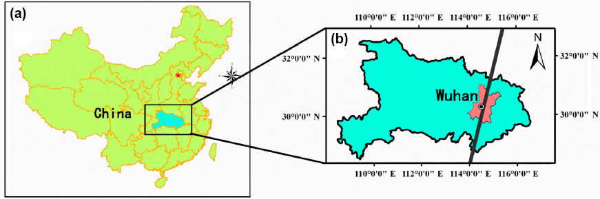
Figure 1Geographic location of the ground-based lidar measurement station. The black point represents the ground-based lidar station. The black line represents the track of CALIPSO satellite.
In this research, we proposed a graphics distribution method (GDM) for deriving the BLH from CALIPSO data and preventing significant reduction of horizontal resolution. The total attenuated backscatter coefficient 532 (TAB532) and attenuated backscatter coefficient 1064 (AB1064) were used for the construction of two-dimensional graphics distribution, which was used for BLH derivation. The GDM algorithm was then tested with real signals under different horizontal smoothing numbers. Finally, the results of BLH obtained by CALIPSO data were compared with those retrieved by the ground-based lidar during January 2013 to December 2017.
2.1 Study area
The CALIPSO ground-based lidar was used for calculation of BLHs over Wuhan, a megacity close to the Han and the Yangtze rivers. Wuhan is one of the most densely populated and industrialised region over central China (B. Liu et al., 2018b; L. Liu et al., 2018; Zhang et al., 2017). In the Wuhan area, the ground-based lidar stations are located at the State Key Laboratory of Information Engineering in Surveying, Mapping and Remote Sensing, Wuhan University (30∘32′ N, 114∘21′ E) (Liu et al., 2017). Figure 1 shows the geographic distributions of the ground-based lidar. The black point represents the ground-based lidar. The black line represents the track of CALIPSO satellite. About matching principles of ground-based and space-borne lidar, the distance between CALIPSO and ground-based lidar stations is within 50 km. Meanwhile, the ground-based lidar data were obtained within 30 min of CALIPSO overpass times.
2.2 Ground-based lidar data
A ground-based lidar system was used for the detection of the atmospheric vertical profiles in Wuhan (Wei et al., 2015). The lidar system uses a pulsed Nd:YAG laser with 532 nm wavelength. The pulse rate of the laser was 20 Hz, and the laser energy was 150 mJ. The vertical resolution of the system was 3.75 m, and the acquisition frequency of the system was 20 Hz. Additional details of this lidar system can be found in previous studies. Given that the lidar signal is susceptible to the noise of background light during daytime, the lidar system was employed at night from 19:00 to 07:00 local time (LT). The ideal profile fitting method proposed by Steyn et al. (1999) is an effective method for delineating stable boundary layers. As this method can be successfully used for obtaining the BLH in ground-based lidar research, an ideal profile fitting method was used. The lidar data were collected from January 2013 to December 2017. After matching the CALIPSO data, the valid number of the ground-based lidar data was 21 cases.
2.3 CALIPSO data
The CALIPSO satellite is the first space-borne lidar optimised for aerosol and cloud profiling, which has a 532 nm channel (parallel and perpendicular polarisation) and a 1064 nm channel (Liu et al., 2009). This satellite can provide the total attenuated backscatter coefficient 532 and attenuated backscatter coefficient 1064 with a horizontal resolution of 1∕3 km and vertical resolution of 30 m. Attenuated backscatter data (Level 1B) were used for testing the proposed algorithm. The cycle time of CALIPSO across the central China region is 16 days, and the crossing time of the satellite in Wuhan is 13:10 and 02:10 LT. The nighttime data have a higher SNR relative to daytime data (Winker et al., 2009; Guo et al., 2016b). The nighttime data were employed for this analysis for the matching of the ground-based data, and cases with cloud and dust were removed in this study. The data collection time was from January 2013 to December 2017. During this time, the total number of CALIPSO crossing Wuhan was 93. After removing the cloud cases, there were 49 valid samples.
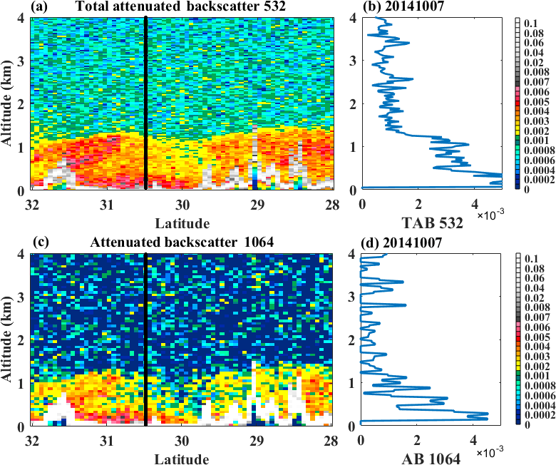
Figure 2(a) Total attenuated backscatter at 532 nm wavelength (TAB532) and (c) the attenuated backscatter at 1064 nm wavelength (AB1064) plot from CALIPSO on 7 October 2014. Panels (b) and (c) indicate the corresponding vertical profile of TAB532 and AB1064 derived from CALIPSO profile over Wuhan area, respectively. The number of horizontal smoothing is 20.
3.1 Method
Previous studies reported that the different particles are distributed in different vertical heights (B. Liu et al., 2018c; Sugimto et al., 2002). Most of the particles above the boundary layer are molecular particles, and the particles below the boundary layer are mainly aerosol particles, as shown in Fig. 2a and c, respectively. Therefore, we proposed a dual-wavelength algorithm that determines BLH on the basis of two-dimensional graphical distribution. The total attenuated backscatter coefficient 532 (TAB532) and attenuated backscatter coefficient 1064 (AB1064) were used to construct the two-dimensional graphical distribution. The specific steps are as follows:
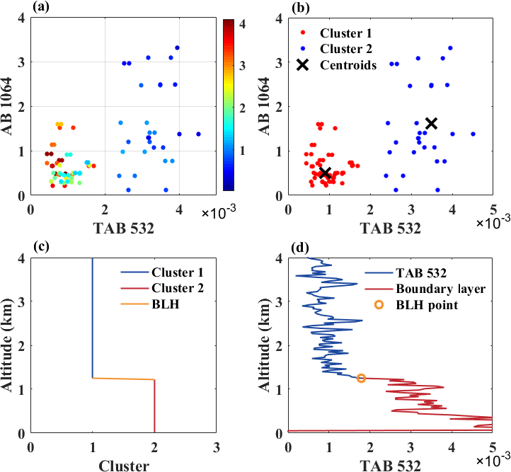
Figure 3Case study over Wuhan area on 7 October 2014. (a) Scatter plots of TAB532 and AB1064. The colour bar shows the altitude of sample point. (b) Classification results. The red and blue point represent the cluster 1 and 2, respectively. The black cross represents the centroid of the cluster. (c) The sequence of category F(z). (d) The result of the case analysis. The orange circle represents the result of BLH.
Firstly, the TAB532 and AB1064 were employed for the construction of the sample sequence X(z). As shown in Fig. 2b and d, the TAB532 and AB1064 represent the aerosol vertical profile at 532 and 1064 wavelength measured by CALIPSO, respectively. The X(z) can be expressed as follows:
where z stands for the altitude of sample points; X(z) represents the coordinates of the sample point at the altitude of z; TAB532(z) and AB1064(z) represent the total attenuated backscatter (532 nm) and attenuated backscatter (1064 nm) value of the sample point at the altitude of z, respectively.
The sample sequence X(z) is shown in Fig. 3a. The colour bar is the altitude of sample points. The figure shows that TAB532 and AB1064 of blue points (the particles below the boundary layer) were larger than those of the red points (the particles above the boundary layer). According to this two-dimensional distribution, the sample sequence X(z) can be divided into two categories.
The k-means method was used for the classification of the sample sequence. Two centroid points (u1, u2) were randomly selected from the sample sequence. For each sample point of sample sequence X(z), the cluster C belonging to it is calculated as follows:
where C(z) represents the cluster of sample point at the altitude of z, and uj is the centroid of cluster j (u1 or u2). For each cluster j, the centroid uj is recalculated as follows:
Equations (3) and (4) are repeated until the centroids (u1 and u2) converge. The sample sequence is divided into two categories after the convergence. As shown in Fig. 3b, cluster2 (blue points) indicates the aerosol particles below the boundary layer, and cluster1 (red points) is the molecular particles above the boundary layer. Black cross represents centroid points. Meanwhile, the category sequence f(z), which changes with height, can be obtained and expressed as follows:
where f(z) is the category of sample point at the altitude of z. The noise points would affect the classification results due to the large noise of satellite data. Therefore, the noise points on the category sequence must be eliminated. The noise point was determined by comparing two points near the point. If the two points above and below this point belong to the same class, then this point should also belong to this category. The noise point can be filtered by
where m represents the multiple of the vertical resolution, and the different values can be selected at different noise levels. When the horizontal smoothing number is small and the signal noise is large, the value of m can be set as 2; when the horizontal smoothing number is large, the value of m can be set as 1. According to the noise removal principle, the the category of noise point was judged as the cluster which is the same as the neighbouring particles. Hence, the noise points were removed, and the new category sequence F(z) was obtained as follows:
where F(z) represents the category of the sample point at the altitude of z. BLH indicates the BLH result. Figure 3c shows the category sequence F(z), which contains the height information and shows evident variation at the top of boundary layer. Therefore, the maximum gradient of the category sequence F(z) is the top point of boundary layer. The BLH can be calculated by searching the maximum gradient, which can be expressed as follows:
Following this process, the BLH was obtained based on the two-dimensional distribution of particles.
3.2 Error analysis
Figure 4 shows the flow chart of the GDM algorithm. Four calculation steps are available: establishing the sample sequence, particle clustering, filtering noise points, and maximum gradient searching. The error of input parameters is the main factor affecting the accuracy of the algorithm because these steps are quantitative calculations. According to the official description, the uncertainty of backscatter coefficient was 20 %–30 % (Winker et al., 2009). The total attenuated backscatter at 532 nm wavelength and the attenuated backscatter at 1064 nm wavelength were measured from CALIPSO. Therefore, the error of input parameters was 20 %–30 %. The error of the BLHs derived by the GDM algorithm is approximately 20 %–30 %. In addition, it needs to be noted that this method cannot be applied to low cloud and dust cases, because the boundary of cloud or dust would be misclassified to BLH. In addition, due to the effect of the nocturnal residual layer, the top of residual layer would be identified as the BLH by lidar system in some cases.
The GDM algorithm was applied to the CALIPSO data acquired from January 2013 to December in 2017. After removing the cases with cloud and dust, the number of residual CALIPSO data over Wuhan area was 49. In addition, the results of BLH were compared with those retrieved by the ground-based lidar.

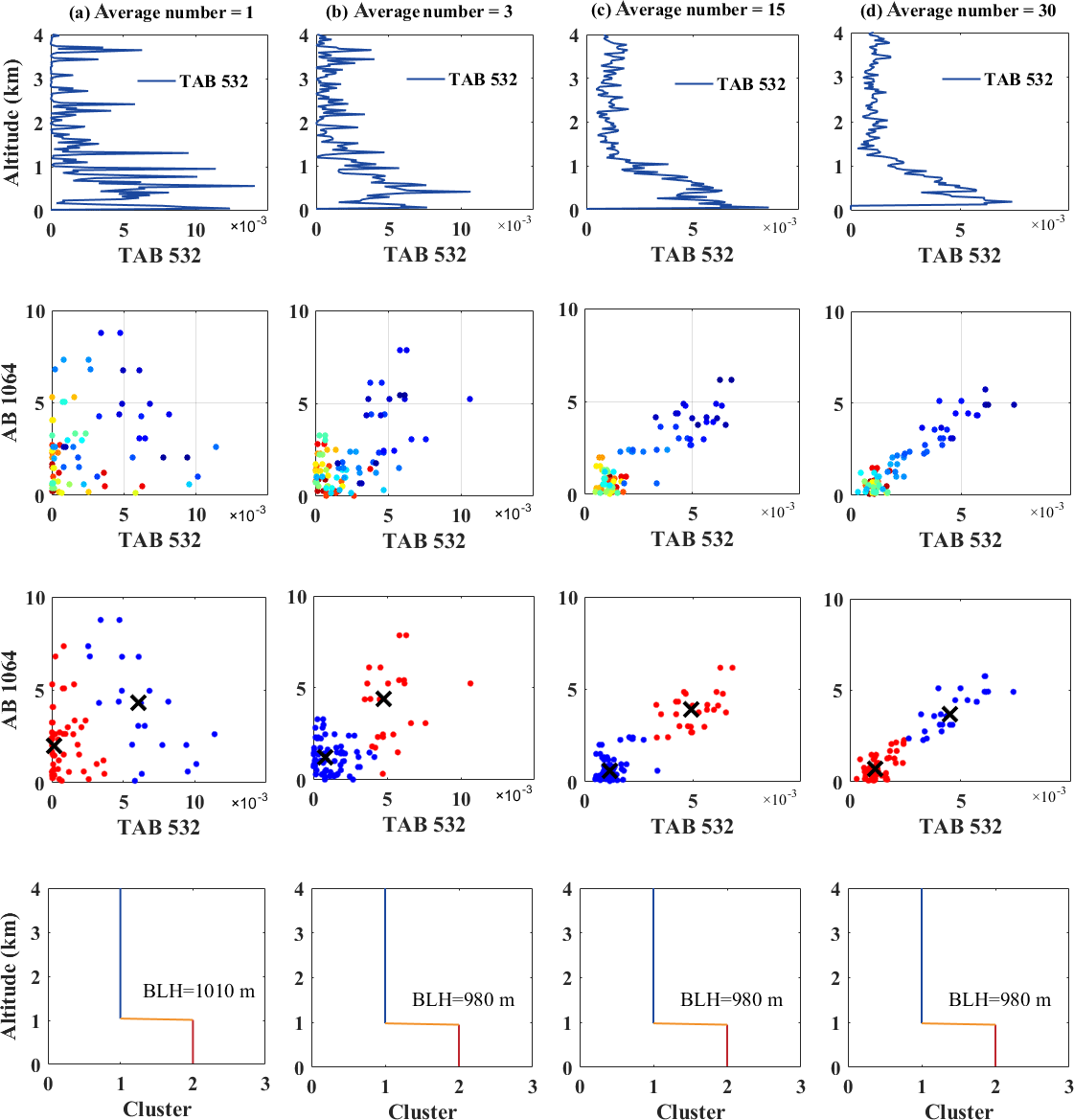
Figure 5Case study of CALIPSO data with different horizontal smoothing numbers on 4 October 2013 over Wuhan area. (a) Average number = 1, (b) average number = 3, (c) average number = 15 and (d) average number = 30. The blue line represents the vertical profile of TAB532 derived from CALIPSO data, the black cross represents the centroid of the cluster and the orange horizontal line represents the BLH result.

Figure 6Case study of CALIPSO data with different horizontal smoothing numbers on 12 February 2015 over Wuhan area. (a) Average number = 1, (b) average number = 3, (c) average number = 15 and (d) average number = 30. The blue line represents the vertical profile of TAB532 derived from CALIPSO data, the black cross represents the centroid of the cluster and the orange horizontal line represents the BLH result.
4.1 Testing with real signals
Figure 5 shows the case study of CALIPSO data with different horizontal smoothing numbers on 4 October 2013 over Wuhan area. Figure 5a, b, c and d represent the vertical profile of TAB532 derived from CALIPSO profile with a horizontal smoothing number of 1, 3, 15 and 30, respectively, and their BLH result was 1020, 980, 980 and 980 m, respectively. Figure 5a shows the vertical profile of TAB532 with a horizontal smoothing number of 1, in which the noise of satellite data was large. Such noise produced discrete sample sequence distribution. However, the category sequence and the BLH result (1010 m) can still be obtained. As shown in Fig. 5b, c and d, the noise of satellite data was reduced with the increase in horizontal smoothing number. Moreover, the vertical profile of TAB532 derived from CALIPSO profile was gradually becoming smooth. Such transformation resulted in significantly compact distribution of sample sequences (Fig. 5d), which were conducive to the classification of sample points. The category sequence was easily obtained from the classification calculation, and the result of the BLH converged to 980 m. In this case, the GDM algorithm can obtain the BLH result under different horizontal smoothing numbers.
Figure 6 shows the case study of CALIPSO data with different horizontal smoothing numbers on 12 February 2015 over Wuhan area. The BLH result of Fig. 6a, b, c and d was 532, 1280, 1370 and 1370 m, respectively. As shown in Fig. 6a, when the horizontal smoothing number was 1, the high noise of CALIPSO mixed together the sample points at different heights. In this condition, the category sequence cannot accurately distinguish between molecular and aerosol particles. Therefore, an inaccurate BLH result was obtained under this condition. When the horizontal smoothing number was added to 3 (Fig. 6b), the distribution of sample sequences significantly improved, and the obtained BLH result was 1280 m. Figure 5c and d show the vertical profile of TAB532 with the horizontal smoothing number of 15 and 30, respectively, in which the distribution of sample sequences gradually became compact. The result of the BLH converged to 1370 m. This result indicates that the GDM algorithm cannot be applied to the data with horizontal smoothing number of 1 in this case, but it can provide a relatively reliable result when the horizontal smoothing number was greater than 3.
The relationship between the horizontal smoothing number and BLH was investigated to determine the convergence of the BLH results. Figure 7 shows the relationship between the horizontal smoothing number and BLH under different cases. Figure 7a shows the case study on 4 October 2013. The result of the BLH converges to 980 m when the horizontal smoothing number was greater than 2. Figure 7b shows the case study on 12 February 2015. The result of the BLH converged to 980 m when the horizontal smoothing number was greater than 4. These results indicate that the PDM algorithm was not applied to the satellite data when the horizontal smoothing number was extremely small. However, this algorithm can provide a reliable result when the horizontal smoothing number is greater than 5.
4.2 Comparison with other algorithms
In this section, we compare the results of BLH obtained by CALIPSO data with those retrieved by the ground-based lidar to verify the stability of the algorithm. The number of the ground-based lidar data matching CALIPSO data was 21. The results of BLH calculated by the MSD method were used as a reference.

Figure 7Relationship between the horizontal smoothing number and BLH under different cases: (a) 4 October 2013 and (b) 12 February 2015.
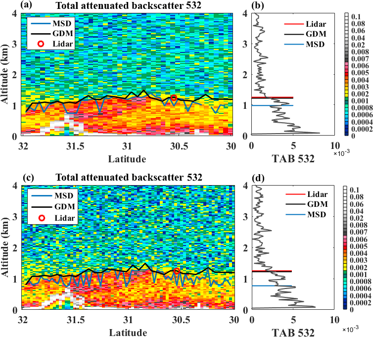
Figure 8Total attenuated backscatter at 532 nm wavelength (TAB532) plot from CALIPSO on 7 October 2014 under the horizontal smoothing number (a) 15 and (c) 9. The corresponding vertical profile of TAB532 derived from CALIPSO profile over Wuhan area under the horizontal smoothing number (b) 15 and (d) 9.
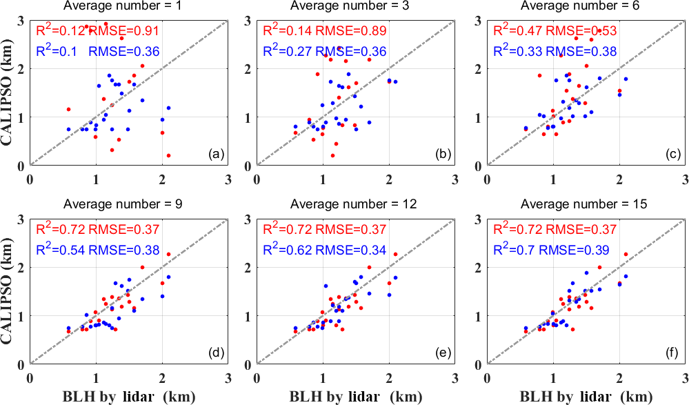
Figure 9Correlation of BLH derived from CALIPSO and ground-based lidar under the horizontal smoothing number of (a) 1, (b) 3, (c) 6, (d) 9, (e) 12 and (f) 15. The red and blue points represent the BLH calculated by GDM algorithm and MSD method, respectively.
Figure 8a and c show the total attenuated backscatter at 532 nm plot from CALIPSO on 7 October 2014 under the horizontal smoothing number 15 and 9, respectively. The black and blue line represent the BLH results calculated by GDM algorithm and MSD method, respectively. The red circle stands for the BLH result from ground-based lidar. Figure 8b shows the corresponding vertical profile of TAB532 derived from CALIPSO profile over Wuhan area under the horizontal smoothing number 15. The BLH results calculated by GDM algorithm, MSD method and ground-based lidar were 1220, 980 and 1250 m, respectively. Figure 8b shows the corresponding vertical profile of TAB532 under the horizontal smoothing number 9. The BLH results calculated by GDM algorithm, MSD method and ground-based lidar were 1220, 770 and 1250 m, respectively.
Figure 9 shows the correlation coefficients between the BLH derived from CALIPSO and ground-based lidar under the horizontal smoothing numbers of 1, 3, 6, 9, 12 and 15. The red and blue points represent the BLH calculated by GDM algorithm and MSD method, respectively. Figure 9a, b and c show the comparison of BLH between CALIPSO and lidar under the horizontal smoothing number of 1, 3 and 6. The correlation coefficients between the BLH derived by GDM algorithm and ground-based lidar were 0.12, 0.14 and 0.47, respectively. Meanwhile, the correlation coefficients between the BLH derived by MSD method and ground-based lidar were 0.1, 0.27 and 0.33. Figure 9d, e and f show the comparison of BLH between CALIPSO and lidar under the horizontal smoothing number of 9, 12 and 15. The correlation coefficients between the BLH derived by GDM algorithm and lidar measurements were both 0.72, and the correlation coefficients between the BLH derived by MSD method and lidar measurements were 0.54, 0.62 and 0.7, respectively. These results indicate that the performance of GDM algorithm was similar to the MSD method when the horizontal smoothing number was large. When the horizontal smoothing number was 9, the performance of GDM algorithm was superior to the MSD method. Moreover, the GDM algorithm and MSD method show a poor performance when the horizontal smoothing number was small.
The CALIPSO satellite is a powerful tool for monitoring the vertical distribution of clouds and aerosols, which offers a significant potential for the estimation of global BLHs from space (Winker et al., 2007, 2009). Moreover, a horizontal smoothing method was used to improve the SNR of satellite data due to its large noise (Guo et al., 2016b; Zhang et al., 2016; Su et al., 2017). However, this method considerably sacrificed the horizontal resolution of CALIPSO detection. A graphics algorithm was proposed to determine the BLHs from CALIPSO data and overcome this problem.
The total attenuated backscatter coefficient 532 and attenuated backscatter coefficient 1064 were used to construct the two-dimensional graphics distribution, as shown in Fig. 3a. The extremum and negative points can be filtered through this graphics distribution. The sample sequence was then classified by the k-means method, and the category sequence was obtained (Fig. 3b). When the horizontal smoothing number was different, the degree of noise was also different. When the noise was large, the noise point which was above the boundary layer may be classified below the boundary layer, thereby significantly affecting the accuracy of category sequence. Therefore, the noise points were removed again, and the new category sequence was obtained (Fig. 3c). The BLH result can be determined from the new category sequence by maximum gradient search (Fig. 3d). The advantage of the GDM algorithm is that this algorithm transforms the gradient solution into graphics distribution solution. The multiple gradient values in the backscatter coefficient profile can be understood as the extremely dispersed distribution of the particles. According to the graphic classification, the influence of noise gradient can be avoided, and a reliable BLH result can be obtained.
The test results of GDM algorithm are shown in Figs. 5, 6 and 7. These results indicate that the GDM algorithm can be applied to the satellite data when the horizontal smoothing number is small. However, when the horizontal smoothing number is below 5, the large noise affects the distribution of the sample sequence, and obtaining the BLH by graphic classification is difficult. Regarding the performance of algorithm, as shown in Figs. 8 and 9, the performance of the GDM algorithm was similar to that of the MSD algorithm when the horizontal smoothing number was large. This finding can be attributed to the noise of satellite data, which produced the evident gradient of aerosol concentration when effectively restrained by the horizontal smoothing method. Thus, both the algorithms can accurately detect the BLH. However, with the decrease in the number of horizontal smoothing, a difference was observed between the GDM and MSD algorithms with respect to performance. When horizontal smoothing number was small (9), the noise of satellite data was ineffectively controlled, thereby resulting in multiple gradients in the vertical direction. The MSD algorithm failed to obtain the effective BLH from the multiple gradient values. However, the GDM algorithm can still detect the BLH based on the graphics distribution, overcome the effect of multiple gradient values and accurately identify the BLH. Therefore, the GDM algorithm can deal well with the CALIPSO data with a small horizontal smoothing number.
We proposed a graphics algorithm to obtain the BLHs from CALIPSO data. The following four calculation steps were used: establishing the sample sequence, particle clustering, filtering noise points and maximum gradient searching. The TAB532 and AB1064 were used for the construction of the two-dimensional graphics distribution. Based on the graphics distribution of atmospheric particulate, the k-means method was used for the classification of the sample sequence and acquisition of the BLH. The algorithm was then applied to the real signals with different horizontal smoothing numbers for the evaluation of the algorithm's performance. The results indicate that the performance of GDM algorithm was poor when the horizontal smoothing number was extremely small (such as 1 to 3), although it can provide a reliable result when the horizontal smoothing number was greater than 5. Finally, the results of BLH obtained by CALIPSO data were compared with those retrieved by the ground-based lidar from January 2013 to December 2017. Notably, when the horizontal smoothing number was extremely large (above 15), the performance of the GDM algorithm was similar to that of the MSD method. It indicated that the 5 km horizontal-resolution CALIPSO data (the horizontal smoothing number of 15) were suitable for both GDM and MSD method to derive the BLH. Moreover, the correlation coefficients between the BLH derived by the GDM method and ground-based lidar were superior to those between the BLH derived by the MSD method and ground-based lidar when the horizontal smoothing number was 9. This finding indicates that the performance of the GDM algorithm is superior to that of the MSD method when the 3 km horizontal-resolution CALIPSO data were used. Overall, the CALIPSO BLH derived by GDM method is reasonably consistent with ground-based lidar. The MSD algorithm can derive the BLH effectively from the 3 and 5 km horizontal resolution CALIPSO data.
The CALIPSO Level 1B data set can be downloaded from https://www-calipso.larc.nasa.gov/tools/data_avail/ (last access: 5 April 2018). Instructions for use and data download methods can be found on the official website. The lidar data at Wuhan station given in this paper are available upon request via email: yym863@gmail.com.
The study was completed with cooperation between all authors. YM and BL designed the research topic, JL and BL conducted the experiment and wrote the paper, and WW, MZ and WG checked the experimental results.
The authors declare that they have no conflict of interest.
This work was supported by the National Key R&D
Program of China (2017YFC0212600), the Haze Program of the Wuhan
Technological Bureau (2017CFB404), and the National Natural Science
Foundation of China (program nos. 41127901 and 41627804).
Edited by: Alexander Kokhanovsky
Reviewed by: two anonymous referees
Bonin, T., Chilson, P., Zielke, B., and Fedorovich, E.: Observations of the early evening boundary-layer transition using a small unmanned aerial system, Bound.-Lay. Meteorol., 146, 119–132, 2013.
Brooks, I. M.: Finding boundary layer top: Application of a wavelet covariance transform to lidar backscatter profiles, J. Atmos. Ocean. Tech., 20, 1092–1105, 2003.
Davis, K. J., Gamage, N., Hagelberg, C. R., Kiemle, C., Lenschow, D. H., and Sullivan, P. P.: An Objective Method for Deriving Atmospheric Structure from Airborne Lidar Observations, J. Atmos. Ocean. Tech., 17, 1455–1468, 2000.
Flamant, C., Pelon, J., and Flamant, P.: Lidar determination of the entrainment zone thickness at the top of the unstable marine atmospheric boundary layer, Bound.-Lay. Meteorol., 83, 247–284, 1997.
Guo, J., Miao, Y., Zhang, Y., Liu, H., Li, Z., Zhang, W., He, J., Lou, M., Yan, Y., Bian, L., and Zhai, P.: The climatology of planetary boundary layer height in China derived from radiosonde and reanalysis data, Atmos. Chem. Phys., 16, 13309–13319, https://doi.org/10.5194/acp-16-13309-2016, 2016a.
Guo, J., Liu, H., Wang, F., Huang, J., Xia, F., Lou, M., and Yung, Y. L.: Three-dimensional structure of aerosol in China: A perspective from multi-satellite observations, Atmos. Res., 178, 580–589, 2016b.
Hennemuth, B. and Lammert, A.: Determination of the atmospheric boundary layer height from radiosonde and lidar backscatter, Bound.-Lay. Meteorol., 120, 181–200, 2006.
Holzworth, G.: Estimates of mean maximum mixing depths in the contiguous United States, Mon. Weather Rev., 92, 235–242, 1964.
Holzworth, G.: Mixing depths, wind speeds and air pollution potential for selected locations in the United States, J. Appl. Meteorol., 6, 1039–1044, 1967.
Huang, Z., Huang, J., Bi, J., Wang, G., Wang, W., Fu, Q., and Shi, J.: Dust aerosol vertical structure measurements using three MPL lidars during 2008 China-US joint dust field experiment, J. Geophys. Res.-Atmos., 115, D00K15, https://doi.org/10.1029/2009JD013273, 2010.
Jordan, N. S., Hoff, R. M., and Bacmeister, J. T.: Validation of Goddard Earth Observing System-version 5 MERRA planetary boundary layer heights using CALIPSO, J. Geophys. Res.-Atmos., 115, D24218, https://doi.org/10.1029/2009JD013777, 2010.
Lange, D., Tiana-Alsina, J., Saeed, U., Tomas, S., and Rocadenbosch, F.: Atmospheric boundary layer height monitoring using a Kalman filter and backscatter lidar returns, IEEE T. Geosci. Remote, 52, 4717–4728, 2014.
Leventidou, E., Zanis, P., Balis, D., Giannakaki, E., Pytharoulis, I., and Amiridis, V.: Factors affecting the comparisons of planetary boundary layer height retrievals from CALIPSO, ECMWF and radiosondes over Thessaloniki, Greece, Atmos. Environ., 74, 360–366, 2013.
Li, H., Yang, Y., Hu, X. M., Huang, Z., Wang, G., Zhang, B., and Zhang, T.: Evaluation of retrieval methods of daytime convective boundary layer height based on lidar data, J. Geophys. Res.-Atmos., 122, 4578–4593, 2017.
Liu, B., Ma, Y., Gong, W., and Zhang, M.: Observations of aerosol color ratio and depolarization ratio over Wuhan, Atmos. Pollut. Res., 8, 1113–1122, 2017.
Liu, B., Ma, Y., Gong, W., Zhang, M., and Yang, J.: Determination of boundary layer top on the basis of the characteristics of atmospheric particles, Atmos. Environ., 178, 140–147, 2018a.
Liu, B., Ma, Y., Gong, W., Zhang, M., and Yang, J.: Study of continuous air pollution in winter over Wuhan based on ground-based and satellite observations, Atmos. Pollut. Res., 9, 156–165, 2018b.
Liu, B., Ma, Y., Gong, W., Jian, Y., and Ming, Z.: Two-wavelength Lidar inversion algorithm for determining planetary boundary layer height. Journal of Quantitative Spectroscopy and Radiative Transfer, 206, 117-124, 2018c.
Liu, J., Huang, J., Chen, B., Zhou, T., Yan, H., Jin, H., and Zhang, B.: Comparisons of PBL heights derived from CALIPSO and ECMWF reanalysis data over China, J. Quant. Spectrosc. Ra., 153, 102–112, 2015.
Liu, L., Guo, J., Miao, Y., Li, J., Chen, D., He, J., and Cui, C.: Elucidating the relationship between aerosol concentration and summertime boundary layer structure in central China, Environ. Pollut., 241, 646–653, 2018.
Liu, Z., Vaughan, M., Winker, D., Kittaka, C., Getzewich, B., Kuehn, R., Omar, A., Powell, K., Trepte, C., and Hostetler, C.: The CALIPSO Lidar Cloud and Aerosol Discrimination: Version 2 Algorithm and Initial Assessment of Performance, J. Atmos. Ocean. Tech., 26, 1198–1213, 2009.
Mamouri, R. E., Amiridis, V., Papayannis, A., Giannakaki, E., Tsaknakis, G., and Balis, D. S.: Validation of CALIPSO space-borne-derived attenuated backscatter coefficient profiles using a ground-based lidar in Athens, Greece, Atmos. Meas. Tech., 2, 513–522, https://doi.org/10.5194/amt-2-513-2009, 2009.
McGrath-Spangler, E. L. and Denning, A. S.: Estimates of North American summertime planetary boundary layer depths derived from space-borne lidar, J. Geophys. Res.-Atmos., 117, D15101, https://doi.org/10.1029/2012JD017615, 2012.
Melfi, S. H., Spinhirne, J. D., Chou, S. H., and Palm, S. P.: Lidar observations of vertically organized convection in the planetary boundary layer over the ocean, J. Clim. Appl. Meteorol., 24, 806–821, 1985.
Reuder, J., Brisset, P., Jonassen, M., Müller, M., and Mayer, S.: The Small Unmanned Meteorological Observer SUMO: A new tool for atmospheric boundary layer research, Meteorol. Z., 18, 141–147, 2009.
Sawyer, V. and Li, Z.: Detection, variations and intercomparison of the planetary boundary layer depth from radiosonde, lidar and infrared spectrometer, Atmos. Environ., 79, 518–528, 2013.
Seibert, P., Beyrich, F., Gryning, S. E., Joffre, S., Rasmussen, A., and Tercier, P.: Review and intercomparison of operational methods for the determination of the mixing height, Atmos. Environ., 34, 1001–1027, 2000.
Steyn, D. G., Baldi, M., and Hoff, R. M.: The detection of mixed layer depth and entrainment zone thickness from Lidar backscatter profiles, J. Atmos. Ocean. Tech., 16, 953–959, 1999.
Su, T., Li, J., Li, C., Xiang, P., Lau, A. K. H., Guo, J., and Miao, Y.: An intercomparison of long-term planetary boundary layer heights retrieved from CALIPSO, ground-based lidar, and radiosonde measurements over Hong Kong, J. Geophys. Res.-Atmos., 122, 3929–3943, 2017.
Sugimoto, N., Matsui, I., Shimizu, A., Uno, I., Asai, K., Endoh, T., and Nakajima, T.: Observation of dust and anthropogenic aerosol plumes in the northwest Pacific with a two-wavelength polarization lidar on board the research vessel Mirai, Geophys. Res. Lett., 29, 1901, https://doi.org/10.1029/2002GL015112, 2002.
Wei, G., Liu, B., Ma, Y., and Miao, Z.: Mie lidar observations of tropospheric aerosol over wuhan, Atmosphere, 6, 1129–1140, 2015.
Winker, D. M., Hunt, W. H., and McGill, M. J.: Initial performance assessment of CALIOP, Geophys. Res. Lett., 34, L19803, https://doi.org/10.1029/2007GL030135, 2007.
Winker, D. M., Vaughan, M. A., Omar, A., Hu, Y., Powell, K. A., Liu, Z., Hunt, W. H., and Young, S. A.: Overview of the CALIPSO mission and CALIOP data processing algorithms, J. Atmos. Ocean. Tech., 26, 2310–2323, 2009.
Yang, D., Li, C., Lau, A. K. H., and Li, Y.: Long-term measurement of daytime atmospheric mixing layer height over Hong Kong, J. Geophys. Res.-Atmos., 118, 2422–2433, 2013.
Zhang, M., Ma, Y., and Gong, W.: Aerosol radiative effect in UV, VIS, NIR, and SW spectra under haze and high-humidity urban conditions, Atmos. Environ., 166, 9–21, 2017.
Zhang, W., Guo, J., Miao, Y., Liu, H., Zhang, Y., Li, Z., and Zhai, P.: Planetary boundary layer height from CALIOP compared to radiosonde over China, Atmos. Chem. Phys., 16, 9951–9963, https://doi.org/10.5194/acp-16-9951-2016, 2016.