the Creative Commons Attribution 4.0 License.
the Creative Commons Attribution 4.0 License.
 | 10 Sep 2018
Validation of the IASI FORLI/EUMETSAT ozone products using satellite (GOME-2), ground-based (Brewer–Dobson, SAOZ, FTIR) and ozonesonde measurements
Anne Boynard
Daniel Hurtmans
Katerina Garane
Florence Goutail
Juliette Hadji-Lazaro
Maria Elissavet Koukouli
Catherine Wespes
Corinne Vigouroux
Arno Keppens
Jean-Pierre Pommereau
Andrea Pazmino
Dimitris Balis
Diego Loyola
Pieter Valks
Ralf Sussmann
Dan Smale
Pierre-François Coheur
Cathy Clerbaux
This paper assesses the quality of IASI (Infrared Atmospheric Sounding Interferometer)/Metop-A (IASI-A) and IASI/Metop-B (IASI-B) ozone (O3) products (total and partial O3 columns) retrieved with the Fast Optimal Retrievals on Layers for IASI Ozone (FORLI-O3; v20151001) software for 9 years (2008–July 2017) through an extensive intercomparison and validation exercise using independent observations (satellite, ground-based and ozonesonde). Compared with the previous version of FORLI-O3 (v20140922), several improvements have been introduced in FORLI-O3 v20151001, including absorbance look-up tables recalculated to cover a larger spectral range, with additional numerical corrections. This leads to a change of ∼4 % in the total ozone column (TOC) product, which is mainly associated with a decrease in the retrieved O3 concentration in the middle stratosphere (above 30 hPa/25 km). IASI-A and IASI-B TOCs are consistent, with a global mean difference of less than 0.3 % for both daytime and nighttime measurements; IASI-A is slightly higher than IASI-B. A global difference of less than 2.4 % is found for the tropospheric (TROPO) O3 column product (IASI-A is lower than IASI-B), which is partly due to a temporary issue related to the IASI-A viewing angle in 2015. Our validation shows that IASI-A and IASI-B TOCs are consistent with GOME-2 (Global Ozone Monitoring Experiment-2), Dobson, Brewer, SAOZ (Système d'Analyse par Observation Zénithale) and FTIR (Fourier transform infrared) TOCs, with global mean differences in the range of 0.1 %–2 % depending on the instruments compared. The worst agreement with UV–vis retrieved TOC (satellite and ground) is found at the southern high latitudes. The IASI-A and ground-based TOC comparison for the period from 2008 to July 2017 shows the long-term stability of IASI-A, with insignificant or small negative drifts of 1 %–3 % decade−1. The comparison results of IASI-A and IASI-B against smoothed FTIR and ozonesonde partial O3 columns vary with altitude and latitude, with the maximum standard deviation being seen for the 300–150 hPa column (20 %–40 %) due to strong ozone variability and large total retrievals errors. Compared with ozonesonde data, the IASI-A and IASI-B O3 TROPO column (defined as the column between the surface and 300 hPa) is positively biased in the high latitudes (4 %–5 %) and negatively biased in the midlatitudes and tropics (11 %–13 % and 16 %–19 %, respectively). The IASI-A-to-ozonesonde TROPO comparison for the period from 2008 to 2016 shows a significant negative drift in the Northern Hemisphere of % decade−1, which is also found in the IASI-A-to-FTIR TROPO comparison. When considering the period from 2011 to 2016, the drift value for the TROPO column decreases and becomes statistically insignificant. The observed negative drifts of the IASI-A TROPO O3 product (8 %–16 % decade−1) over the 2008–2017 period might be taken into consideration when deriving trends from this product and this time period.


Ozone (O3) plays a major role in the chemical and thermal balance of the atmosphere. In the stratosphere, O3 protects the biosphere and humans from harmful ultraviolet (UV) radiation. In the troposphere, O3 plays different roles depending on altitude. Near the surface, ozone in excessive amounts is one of the main air pollutants impacting both human health (Brunekreef and Holgate, 2002; Lim et al., 2012) and ecosystems (Fowler et al., 2009). In the upper troposphere, ozone is an important anthropogenic greenhouse gas (IPCC, 2013) and acts as a short-lived climate forcer (Shindell et al., 2012). Tropospheric O3 originates either from complex photochemical reactions involving nitrogen oxides (NOx), carbon monoxide (CO) and hydrocarbons (e.g., Chameides and Walker, 1973; Crutzen, 1973) or from the stratosphere by downward transport to the troposphere especially at mid- and high- latitudes (e.g., Holton et al., 1995) as well as from long-range transport (e.g., Stohl and Trickl, 1999). The lifetime of tropospheric ozone varies with altitude and ranges from 1 to 2 days in the boundary layer, where dry deposition is the major sink, to several weeks in the free troposphere, meaning that the transport scale of O3 can be intercontinental and hemispheric (Monks et al., 2015). Therefore, to better understand its variability and impacts, it is crucial to obtain information on its vertical, spatial and temporal distribution. This information can be provided by observations from spaceborne instruments.
The Infrared Atmospheric Sounding Interferometer (IASI) is a nadir-viewing spectrometer (Clerbaux et al., 2009, 2015) that has been flying on board the EUMETSAT's (European Organisation for the Exploitation of Meteorological Satellites) Metop-A and Metop-B satellites, since October 2006 and September 2012, respectively. In order to ensure the continuity of IASI observations for atmospheric composition monitoring, a third satellite (Metop-C) is scheduled to be launched in November 2018. Thanks to the nadir geometry complemented by off-nadir measurements of up to 48.3∘ on both sides of the satellite track (swath of about 2200 km), each IASI instrument covers the globe twice a day, with a field of view of 4 pixels of 12 km in diameter on the ground at nadir. The two Metop satellites are on the same orbit with Equator crossing times of 09:30 (21:30) local mean solar time for the descending (ascending) part of the orbit. Therefore, there are numerous common observations between two consecutive tracks. However, as Metop-A and Metop-B are 180∘ out of phase, there is a ∼50 min temporal difference between both instruments (one satellite might be before or after the other); thus, the observations are never quite simultaneous. In addition, the geometry of the observations is different and generally off-nadir with opposite angles, meaning that the location of the observation between the two instruments varies and the pixels are not absolutely geographically co-localized.
With a twice daily coverage and a 12 km diameter footprint at nadir, IASI has the potential to provide global O3 measurements with a high spatial resolution. Previous studies have demonstrated IASI's ability to measure O3 separately in the stratosphere (Scannell et al., 2012; Gazeaux et al., 2013), in the upper troposphere and lower stratosphere (UTLS) (e.g., Barret et al., 2011; Wespes et al., 2016), and in the troposphere (e.g., Eremenko et al., 2008; Dufour et al., 2010, 2015; Safieddine et al., 2013, 2014). Using the long-term IASI O3 record, the interannual variability of tropospheric ozone and long-term trends can be derived (Safieddine et al., 2016; Wespes et al., 2016, 2018; Gaudel et al., 2018). Recently, Wespes et al. (2017) analyzed more than 8 years of IASI O3 data to identify the main geophysical drivers (e.g., solar flux, the Quasi-Biennial Oscillation, the North Atlantic Oscillation, the El Niño–Southern Oscillation) of O3 regional and temporal variability.
Several research groups have developed O3 retrieval algorithms for IASI based on different approaches (e.g., Barret et al., 2011; Dufour et al., 2012; Hurtmans et al., 2012; Oetjen et al., 2016). In particular, ULB & LATMOS have developed the Fast Optimal Retrievals on Layers for IASI O3 (FORLI-O3) software (Hurtmans et al., 2012), which uses the IASI Level 1C data to retrieve Level 2 O3 products. A series of validation exercises of IASI O3 products retrieved from different versions of FORLI- O3 (v20100825, v20140922), focusing on a particular region and/or relatively short period of time, were undertaken (e.g., Dufour et al., 2012; Pommier et al., 2012; Scannell et al., 2012; Gazeaux et al., 2013; Safieddine et al., 2016). Boynard et al. (2016) performed an extensive validation of IASI O3 products retrieved from FORLI-O3 v20140922 against a series of independent observations, on the global scale, for the period from 2008 to 2014. This study reported that, on average, FORLI-O3 v20140922 overestimates the ultraviolet (UV) total ozone column (TOC) by 2 %–7 % with the largest differences found at high latitudes. It is worth mentioning that Boynard et al. (2016) did not perform any comparison with measurements in spectral ranges other than the UV. The comparison with ozonesonde vertical profiles shows that, on average, FORLI-O3 v20140922 underestimates O3 by ∼5 %–15 % in the troposphere, while it overestimates O3 by ∼10 %–40 % in the stratosphere depending on the latitude.
Several algorithm improvements were introduced later in FORLI-O3, including absorbance look-up tables recalculated to cover a larger spectral range using the 2012 HITRAN spectroscopic database (Rothman et al., 2013), with additional numerical corrections. Boynard et al. (2016) evaluated 12 days of the new IASI O3 products retrieved from FORLI v20151001 and found a correction of ∼4 % for the TOC positive bias when compared to the UV ground-based (GB) and satellite observations, bringing the overall global comparison to ∼1 %–2 % on average. It was shown that this improvement is mainly associated with a decrease in the retrieved O3 concentration in the middle stratosphere (MS, above 30 hPa/25 km). This O3 retrieval algorithm (FORLI-O3 v20151001) is currently being implemented in the EUMETSAT processing facility under the auspices of the “Ozone and Atmospheric Composition Monitoring Satellite Application Facility” (AC SAF) project in order to operationally distribute Level 2 IASI O3 profiles to users through the EUMETCast system in 2018. IASI Level 2 and Level 3 O3 products processed with FORLI v20151001 are part of the European Space Agency O3 Climate Change Initiative (Ozone_cci, http://www.esa-ozone-cci.org, last access: 30 August 2018) and the European Centre for Medium-Range Weather Forecasts (ECMWF) Copernicus Climate Change (C3S) projects, respectively. These programs focus on building consolidated climate-relevant ozone datasets as essential climate variables (ECVs). Therefore, validating the latest version of the IASI O3 products over a long time period and assessing their stability are necessary for decadal trend studies, model simulation evaluation and data assimilation applications. This is one of the main motivations of the present work. The goals of the Ozone_cci project are described in Garane et al. (2018) whilst its requirements in term of satellite product stability, which is defined as 1 %–3 % decade−1 based on the requirements formulated by the Global Climate Observing System (GCOS) and the “Climate Modelling User Group” (CMUG) climate modeling community for ozone, are detailed in Van Weele et al. (2016).
In this paper, we assess the quality of the IASI O3 products retrieved using FORLI-O3 v20151001 (hereafter referred as to “IASI O3 products”), with GOME-2 (Global Ozone Monitoring Experiment-2; also on Metop), ground-based network data (Brewer, Dobson, SAOZ – Système d'Analyse par Observation Zénithale – and FTIR – Fourier transform infrared) and ozonesonde measurements. Sections 2 and 3 describe the characteristics of the datasets used for the validation and the comparison methodology, respectively. Section 4 presents the intercomparison between IASI-A and IASI-B O3 derived total and tropospheric columns. Section 5 provides the IASI-A and IASI-B TOC and partial ozone column product validation results using independent satellite, GB and ozonesonde observations. Finally, Section 6 summarizes the results from this new validation.
2.1 IASI ozone retrievals
IASI ozone retrievals are performed in the 1025–1075 cm−1 spectral range using the optimal estimation method (OEM) (Rodgers, 2000) and tabulated absorption cross sections at various pressures and temperatures to speed up the radiative transfer calculation. The ozone climatology by McPeters et al. (2007) is used as a priori information consisting of one single O3 a priori profile and variance–covariance matrix. The EUMETSAT Level 2 data (pressure, water vapor, temperature and clouds) are used as input in FORLI. It is worth mentioning that the EUMETSAT dataset is not homogenous, as it has been processed using different versions of the IASI Level 2 Product Processing Facility between 2008 (v4.2) and 2016 (v6.2), as summarized in Van Damme et al. (2017). The error budget of the retrieved O3 profile shows that the dominant errors originate from the limited vertical sensitivity, from the measurement noise and from uncertainties in the fitted (water vapor column) or fixed (e.g., surface emissivity, temperature profile) parameters (Hurtmans et al., 2012). In order to avoid cloud contaminated scenes, retrievals are only performed for clear or almost-clear scenes with a fractional cloud cover below 13 %, identified using the cloud information from the EUMETSAT operational processing (August et al., 2012). In addition, no retrieval is performed for pixels characterized by an error related to the Level 1C IASI data, by missing Level 2 EUMETSAT data associated with Level 1C data or when temperature, water vapor, surface pressure or cloud values are missing in Level 2 EUMETSAT data.
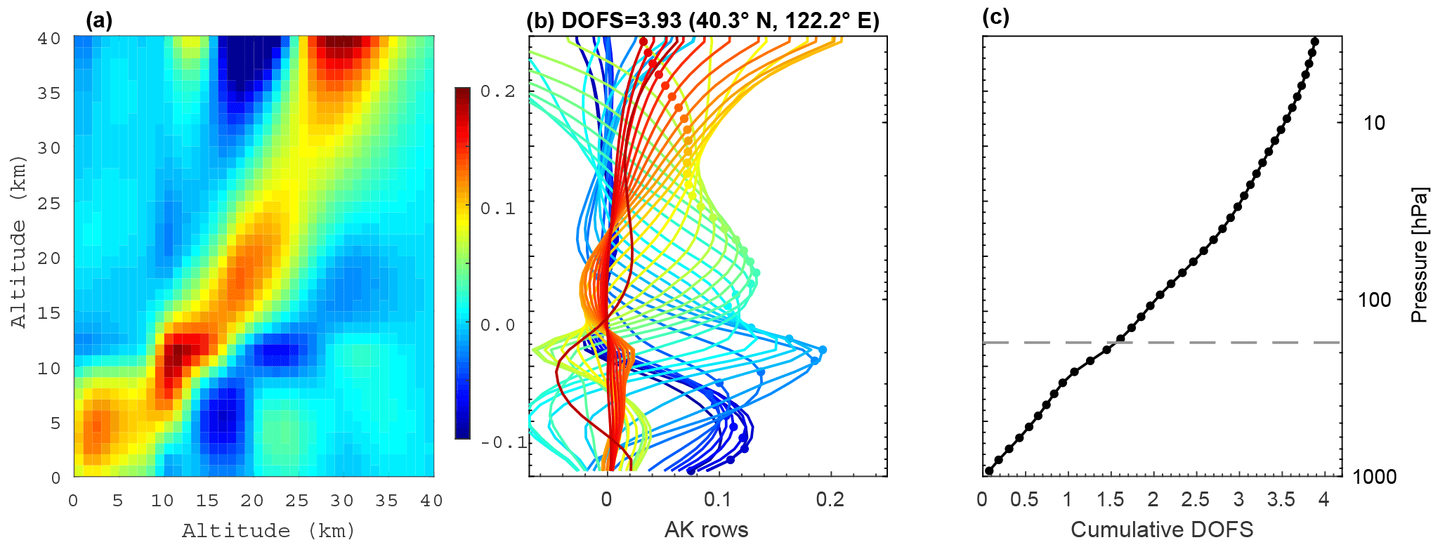
Figure 1(a) Example of the averaging kernel (AK) matrix for the IASI-A vertical profile retrieval indicating where the information present in the IASI-A vertical ozone profile (horizontal axis) originates from in the atmosphere (vertical axis). (b) Another representation of the AK matrix (each line is a row of the AK matrix); the nominal height of each kernel is marked by a circle. (c) Cumulative DOFS (degree of freedom for signal) obtained from the diagonal of the AK matrix. The AKs expressed in (molecules cm−2)/(molecules cm−2) correspond to one daytime midlatitude measurement (40.3∘ N, 122.2∘ E) obtained on 1 June 2016 for each of the 1 km retrieved layers from the surface to an altitude of 40 km.
The IASI O3 dataset used in this paper covers the period from January 2008 to July 2017. The O3 product is a vertical profile given as partial columns in molecules per square centimeter in 40 layers between the surface and 40 km, with an extra layer from 40 km to the top of the atmosphere. It also includes other relevant information such as quality flags, the a priori profile, the total error profile and the averaging kernel (AK) matrix, on the same vertical grid. Quality flags were applied to filter the dataset for further validation analysis, and data were excluded under the following specific conditions: (i) when the spectral fit residual root mean square error (RMS) was higher than W (cm2 sr cm−1)−1, reflecting a difference that was too large between observed and simulated radiances; (ii) when the spectral fit residual bias was lower than W (cm2 sr cm−1)−1 or higher than W (cm2 sr cm−1)−1; (iii) when the partial O3 column was negative; (iv) when there were abnormal averaging kernel values; (v) when the spectral fit diverged; (vi) when the total error covariance matrix was ill conditioned; (vii) when the O3 profiles had an unrealistic C-shape (i.e., abnormal increase in O3 at the surface, such as over desert due to emissivity issues), with a ratio of the surface–6 km column to the total column higher than or equal to 0.085 and (viii) when the DOFS (degree of freedom for signal) was lower than 2, which was mostly associated with bad quality data in the Antarctic region.
A representative IASI-A averaging kernel matrix is illustrated in Fig. 1a, showing the difficulty involved with distinguishing the ozone structures between one level and another. However, it also shows the altitude ranges characterized by peaks of sensitivity: ∼5, 12, 18 and 40 km. Another way to visualize the AK matrix is to represent the AK profiles as a function of altitude as shown in Fig. 1b. The AK are not maximal at their nominal altitudes, which indicates that other altitudes contribute to the ozone value at the individual retrieval altitude. A way to estimate the vertical resolution of IASI O3 profiles is to analyze the DOFS as a function of altitude. The cumulative DOFS, which is presented in Fig. 1c, continuously increases with altitude, given that there is information in the observations for the entire range of altitudes.
The IASI retrieval error on the TOC, including the smoothing and the measurement error, is usually below 2 %, except in the Antarctic (>4 %), which is due to the particularly weak signal in this region; for the surface–300, 300–150, 150–25 and 25–3 hPa partial columns, it is estimated to be ∼15 %, 17 %, 4 % and 3 %, respectively.
2.2 The Global Ozone Monitoring Experiment-2 (GOME-2) data
The GOME-2 instrument, also on board the Metop-A and B platforms, is a UV–vis–NIR (visible–near IR) nadir viewing scanning spectrometer, with an across-track scan time of 6 s and a nominal swath width of 1920 km, which provides global coverage of the sunlit part of the atmosphere within a period of approximately 1.5 days (Hassinen et al., 2016; Munro et al., 2016). GOME-2 ground pixels have a footprint size of 80 km × 40 km, which is larger than that of IASI (pixel diameter of 12 km). In the framework of the EUMETSAT AC SAF project, GOME-2 total ozone data are processed at DLR (Deutsches Zentrum für Luft- und Raumfahrt) operationally, both in near real time and offline, using the GOME Data Processor (GDP) algorithm (Loyola et al., 2011; Hao et al., 2014; Valks et al., 2014). The GOME-2 products have been validated using ground-based measurements (e.g., Loyola et al., 2011; Koukouli et al., 2012, 2015; Hao et al., 2014), which have shown an overall agreement within 1 % in most situations. As shown in Hao et al. (2014), there is an excellent agreement between the GOME-2A and GOME-2B TOCs, with a mean difference of around 0.5 %. Therefore, in this study, the IASI-A and IASI-B validation is limited to the comparison with GOME-2A TOC products. In this comparison, we only use GOME-2A TOC data meeting the valid conditions given in Valks et al. (2017): a TOC value ranging between 75 and 700 Dobson units (DU) and a slant column error low than 2 %.
2.3 Ground-based data
Daily TOC measurements from Dobson and Brewer UV spectrophotometers available for the period from 2008 to 2017 were downloaded from the World Ozone and Ultraviolet Radiation Data Centre (WOUDC, http://woudc.org, last access: 15 December 2017). The GB stations considered in this paper (see Table A1 in Boynard et al., 2016 for a complete list of the stations) have been extensively used in a series of validation papers regarding satellite TOC measurements (e.g., Weber et al., 2005; Balis et al., 2007a, b; Koukouli et al., 2012, 2015; Boynard et al., 2016). For the validation of IASI-A and IASI-B TOCs, only direct sun observations are used as GB UV reference data as they are the most reliable for both the Dobson and the Brewer spectrophotometers, the latter offering an accuracy of about 1 % at moderate solar zenith angles (e.g., Kerr, 2002).
TOC measurements are also obtained from SAOZ zenith sky UV–vis spectrometers (Pommereau and Goutail, 1988), which are part of the Network for the Detection of Atmospheric Composition Change (NDACC, http://www.ndacc.org, last access: 22 December 2017). The SAOZ TOC measurements are performed in the visible Chappuis bands between 450 and 550 nm with a medium spectral resolution of 1 nm, and take place twice a day during twilight (sunrise and sunset) at solar zenith angles ranging between 86 and 91∘. The retrieval is based on the differential optical absorption spectroscopy (DOAS) procedure (Platt, 1988). Since observations are performed at twilight, SAOZ can be operated throughout the year at all latitudes up to ±67∘. At latitudes higher than the polar circle, there is no measurement during permanent night in winter and during permanent day in summer. SAOZ performances have been continuously assessed by regular comparisons with UV–vis independent observations (e.g., Hofmann et al., 1995; Roscoe et al., 1999; Hendrick et al., 2011). The SAOZ total accuracy, including a 3 % cross-section uncertainty, is ∼6 % (Hendrick et al., 2011). In this study, eight SAOZ stations deployed at latitudes from the Arctic to the Antarctic (see Table 3 in Boynard et al., 2016 for their locations) are used for IASI-A and IASI-B TOC validation.
Regular ozone measurements from high-resolution solar absorption spectra recorded by GB FTIR (Fourier transform infrared) spectrometers available for the period from 2008 to 2017 were downloaded from NDACC. The ozone FTIR retrieval principle, which is based on the optimal estimation method (Rodgers, 2000), as for FORLI, is detailed in Vigouroux et al. (2008). Measurements such as these have the advantage of providing not only TOCs with a precision of 2 %, but also low vertical resolution profiles with about four independent partial columns: one in the troposphere and three in the stratosphere up to about 45 km, with a precision of about 5 %–6 % (Vigouroux et al., 2015). Therefore, the FTIR measurements are used to validate not only IASI TOCs but also IASI partial ozone columns. The stations considered in the present work were used in several papers for trend analyses (Vigouroux et al., 2008, 2015; García et al., 2012; Wespes et al., 2016) and validation studies (Dupuy et al., 2009; Viatte et al., 2011). The latitudinal coverage ranges from 67.8∘ N to 45∘ S, so only the southern high latitudes are not covered. The locations of the six FTIR stations used in the comparison are given in Table 1 and presented in Fig. 2. Since these solar absorption measurements require daylight conditions, there is no measurement at Kiruna during polar winter. All stations use the high-resolution spectrometers from Bruker, which can achieve a resolution of 0.0035 cm−1 or better. Details on the harmonized retrieval parameters can be found in Vigouroux et al. (2015). For all stations, the 10 µm spectral region is fitted to retrieved O3 using two retrieval algorithms: either PROFFIT9 at Kiruna and Izaña or SFIT2/4 at the other stations. The two algorithms have been compared in Hase et al. (2004). The spectroscopic database used is HITRAN 2008 (Rothman et al., 2009). Each station uses the daily pressure and temperature profiles from NCEP (National Centers for Environmental Prediction) and has one a priori profile, which is obtained from the same model, WACCM4 (Whole Atmosphere Community Climate Mode; Garcia et al., 2007).
2.4 Ozonesonde data
High resolution ozone vertical profiles measured from ozonesonde for the period from 2008 to 2017 were downloaded from the WOUDC and NOAA-ESRL (http://www.esrl.noaa.gov/gmd/dv/ftpdata.html, last access: 17 December 2017) archives. The sondes provide measurements of O3 up to 30–35 km with a vertical resolution of ∼150 m. Only sonde measurements based on electrochemical concentration cells (ECCs), which measure the oxidation of a potassium iodine (KI) solution by O3 (Komhyr et al., 1995), were used in this study. Their accuracy is generally good (±3 %–5 %) and their uncertainties are of about 10 % throughout most of the profile below 28 km (Deshler et al., 2008; Smit et al., 2007), while other types of ozonesondes have a somewhat poorer accuracy (5 %–10 %) (e.g., Hassler et al., 2014; Liu et al., 2013). A total of 56 ozonesonde stations in midlatitudes, polar and tropical regions are considered in the present study. The locations of the ozonesonde stations used in the comparison are presented in Fig. 2.
Table 1List of the FTIR stations used for the validation of IASI TOCs and partial ozone columns. The latitude, longitude and altitude above sea level in kilometers (km a.s.l.) are provided for each station.
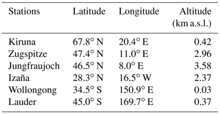

Figure 2Spatial distribution of ozonesonde and FTIR stations used in this study. The different colors represent the mean biases in Dobson units (DU) between IASI-A and sonde TROPO O3 columns (defined as the surface–300 hPa column) at each station and the dot size represents the standard deviation. The average is performed for the period from January 2008 to July 2017. The mean bias between the IASI-A and FTIR TROPO O3 columns is indicated by the dots circled in magenta.
Since the characteristics are not the same from one dataset to another, different comparison methodologies and collocation criteria are applied and described in this section. For all datasets, the differences are calculated as: [IASI − DATA] (in DU) or [100 × (IASI − DATA) ∕ DATA] (in percent, %), where DATA corresponds to the independent data used for the validation of the IASI ozone data (i.e., GOME-2, Brewer–Dobson, SAOZ, FTIR and sonde ozone data).
The IASI-A and IASI-B O3 products are assessed in terms of TOCs and partial ozone columns. The validation exercise is performed using the same partial columns as those used in Wespes et al. (2016). These columns are used because they contain around one piece of information, have maximum sensitivity approximately in the middle of each of the layers and reproduce the well-known cycles related to chemical and dynamical processes characterizing the following layers: surface–300 hPa (TROPO), 300–150 hPa (UTLS), 150–25 hPa (LMS for lower and middle stratosphere) and 25–3 hPa (MS). On average, these pressure columns correspond to the following altitude columns: surface–8, 8–15, 15–22 and 22–40 km, respectively. However, it should be noted that for the comparison between IASI and ozonesonde data, the MS is limited to the 25–10 hPa column as sonde generally burst around 30–35 km (see Sect. 3.2 below). For the assessment of IASI vertical profiles, we refer to Keppens et al. (2018, this issue).
The comparison of IASI-A and IASI-B against DATA is performed over the period from 2008 to 2017 and 2013 to 2017, respectively.
3.1 Direct comparison with GOME-2, Brewer, Dobson and SAOZ data
Since only the TOCs are provided in the independent GOME-2A, Brewer, Dobson and SAOZ datasets, a direct IASI/DATA comparison is performed in this validation exercise.
The comparison of IASI and GOME-2A TOCs is not straightforward because the pixels are not co-localized in time and space and the IASI and GOME-2 instruments have a different pixel size. In order to compare collocated data, a simple method is to calculate the daily average of IASI-A, IASI-B and GOME-2A TOCs along with their relative difference over a constant grid cell. As the UV–vis instrument provides daytime observations, only the IASI daytime data (SZA < 90∘) are used in this comparison.
For the comparison of IASI against Brewer and Dobson TOCs, the coincidence criteria are set to a 50 km search radius between the satellite pixel center and the geo-colocation of the ground-based station as well as to the same day of observations. For each GB measurement, only the closest IASI measurements are kept for the comparison.
For the comparison of IASI against SAOZ TOCs, sunrise (sunset) SAOZ measurements are compared to collocated daytime (nighttime) IASI daily data averaged in a 300 km diameter semi-circular area located to the east (west) of the ground-based station. Note that since similar results are found for daytime and nighttime measurements, only comparisons for daytime data are shown in the following.
3.2 Comparison with FTIR and ozonesonde data
For the comparison of IASI data against FTIR and sonde TOCs and partial ozone columns, the coincidence criteria used in this study are the same as those defined in Boynard et al. (2016), except for the time coincidence which is slightly different in order to be more consistent with the temporal variability of tropospheric ozone: we apply coincidence criteria of a 100 km search radius and ±6 h. As the ozonesonde measurements are mainly performed in the morning (local time), this implies that most of the pixels meeting these coincidence criteria correspond to pixels of the IASI morning overpass, which is not the case for FTIR measurements that can be performed throughout the day.
In the comparison with FTIR data, the FTIR retrieved profiles are adjusted following Rodgers and Connor (2003, their Eq. 10) in order to take the different a priori profiles used in both IASI and FTIR retrievals into account:
where AFTIR is the FTIR AK matrix, I is the unity matrix, and xa,FTIR and xa,IASI are the respective FTIR and IASI O3 a priori profiles.
In addition, when validating satellite profile products, a proper comparison method is used to account for the difference in vertical resolution. In the present work, the ozonesonde and adjusted FTIR profiles are first interpolated on the corresponding IASI vertical grid and then degraded to the IASI vertical resolution by applying the IASI AKs and a priori O3 profile according to Rodgers (2000):
where xs is the smoothed ozonesonde/FTIR profile, xraw is the ozonesonde/adjusted FTIR profile interpolated on the IASI vertical grid (referred as “raw” FTIR), xa is the IASI a priori profile and A is the IASI AK matrix. Incomplete ozonesonde profiles above ozonesonde burst altitude are filled with the a priori profile.
For each ozonesonde/FTIR measurement, we calculate the TOCs (only for the FTIR data) and the four partial columns defined above from all IASI and smoothed ozonesonde/FTIR profiles meeting the coincidence criteria. We then average all IASI and smoothed ozonesonde/FTIR total and partial columns. Once this has been carried out there is one IASI–DATA profile pair per ozonesonde/FTIR measurement. To avoid unrealistic statistics, skewed by extremely unrealistic, low values in the UTLS O3 columns found in the smoothed ozonesonde data, we filter out extreme outliers exceeding 200 % relative differences with IASI (which can be up to ∼8 % of the data in the tropical UTLS).

Figure 3Contour representation of the relative difference (in percent) between IASI-A and IASI-B total ozone column (TOC) products for the 1∘ zonal monthly mean TOCs for the period from May 2013 to July 2017 for daytime data (a) and nighttime data (b). The relative differences are calculated as 100× (IASI-A − IASI-B) ∕ IASI-A.
Before validating IASI-A and IASI-B O3 products, we assess the consistency between both instruments over the common period from May 2013 to July 2017. For the intercomparison exercise, we first calculate the daily IASI-A and IASI-B averages over a grid. Then for each grid cell, we calculate the relative difference as 100× [(IASI-A − IASI-B) ∕ IASI-B]. Finally we calculate the monthly averaged data from the daily gridded differences. A statistical analysis of IASI-A and IASI-B TOCs and TROPO O3 columns is performed with respect to time and latitude.
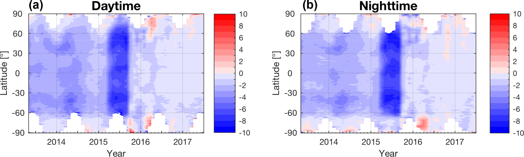
Figure 4Same as Fig. 3 but for the TROPO O3 column products (defined as the column integrated between the surface and 300 hPa).
Figure 3 illustrates the 1∘ zonal monthly relative differences between IASI-A and IASI-B TOCs (computed from daily gridded differences) for daytime measurements (Fig. 3a) and nighttime measurements (Fig. 3b). IASI pixels are considered as daytime or nighttime data if the solar zenith angle (SZA) is <90∘ or ≥90∘, respectively. An excellent agreement between both IASI-A and IASI-B TOCs is observed, with differences within 0.4 %, except for the polar regions. As previously discussed in Boynard et al. (2016), a possible reason for the larger differences in polar regions is the combination of the overlap of consecutive orbits with different times, which equates to different meteorological conditions. Metop, with its polar orbit, makes 14 revolutions per day and passes by the poles on each revolution. This leads to a larger number of observations over the poles each day at different local times for the same grid cell. Therefore, the variability in O3 is much larger leading to both larger differences between the measurements and a larger standard deviation (not shown). Two interesting features that can be noted from Fig. 3 are (i) the slight increase in the differences in 2015 (April–September) and the decrease in the differences between the period prior to April 2015 and the period after September 2015. These two points will be discussed in the following.
Figure 4 illustrates the 1∘ zonal monthly relative differences between IASI-A and IASI-B TROPO O3 columns (computed from daily gridded data) for daytime measurements (Fig. 4a) and nighttime measurements (Fig. 4b). In general, the differences between IASI-A and IASI-B TROPO O3 columns are within ±2 % although larger differences can be found locally, especially in the polar regions. As for the TOCs product, the differences decrease from October 2015 with respect to the period from May 2013 to April 2015, and the differences are significantly larger for the period from April to September 2015 (up to 10 %). Another noticeable feature during the period from April to September 2015 is the opposite signs between the differences in TOCs (Fig. 3) and the differences in TROPO O3 columns (Fig. 4).
The reason for these unexpected differences lies in the fact that on 13 April 2015, there was an error in the IASI-A pixel registration, which slightly modified the IASI-A viewing angle (Buffet et al., 2016). This was corrected in September 2015 and produced a ∼5-month period (between April and September 2015) with somewhat larger differences observed between IASI-A and IASI-B O3 products. Furthermore, on 7 October 2015, the IASI's cube corner compensation device, which was shown to generate micro-vibrations and random errors in the IASI spectra, was stopped. As a result, since October 2015, the IASI-A and IASI-B spectra are of better quality/stability (Buffet et al., 2016; Jacquette et al., 2016).
Because of the changes made in the IASI-A Level 1 data processing, the comparison statistics are performed over two periods, excluding the period between April and September 2015. Over the period from May 2013 to March 2015, the IASI-A TOC product measures 0.3±1.1 % less ozone than IASI-B for both daytime and nighttime measurements. From October 2015, as expected, the overall differences and standard deviation are smaller: the IASI-A TOC product measures 0.1±0.5 % less ozone than IASI-B. Similar results are found for the TROPO O3 column: before April 2015, the IASI-A TROPO O3 product measures 2.4±0.5 % and 2.1±0.4 % less ozone than IASI-B for daytime and nighttime measurements, respectively. From October 2015, the overall difference between both instruments decreases and is equal to 1.4±1.3 %.
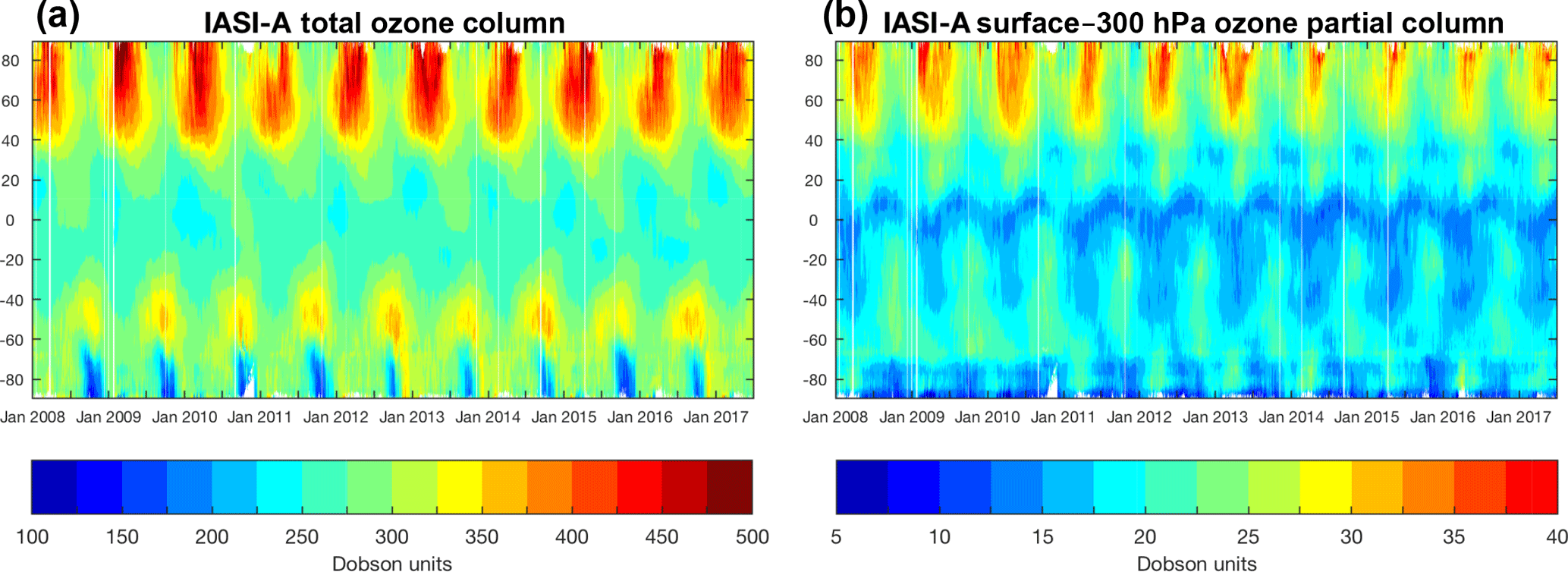
Figure 5IASI-A total ozone column (a) and TROPO O3 column (b) record (in Dobson units) as a function of latitude and time from January 2008 to July 2017. The TROPO O3 column is calculated as the column integrated between the surface and 300 hPa.
The excellent agreement between the current IASI-A and IASI-B TOC and TROPO O3 columns (April–September 2015 excluded) allows the combined use of IASI-A and IASI-B instruments to provide homogeneous total and tropospheric ozone data with full daily global coverage measurements. Whilst the IASI-B O3 products for the period from April to September 2015 are better suited for high quality use, it is worth noting that the IASI-A instrumental issue only affects the TOC by 0.4 % and the tropospheric ozone by 10 %. These differences are much lower than the TOC and tropospheric retrieval errors estimated to 2 % and 15 % on average, respectively, justifying the potential use of the IASI-A data over the April–September 2015 period if it is required. In the validation exercise presented in the next section, the period from April to September 2015 is included.

Figure 6(a) Relative differences (in percent) between IASI-A and GOME-2A for 1∘ zonal monthly mean total ozone columns during the 2008–2017 period; (b) the associated standard deviation (in percent). The relative difference is calculated as 100× (IASI-A − GOME-2A) ∕ GOME-2A.
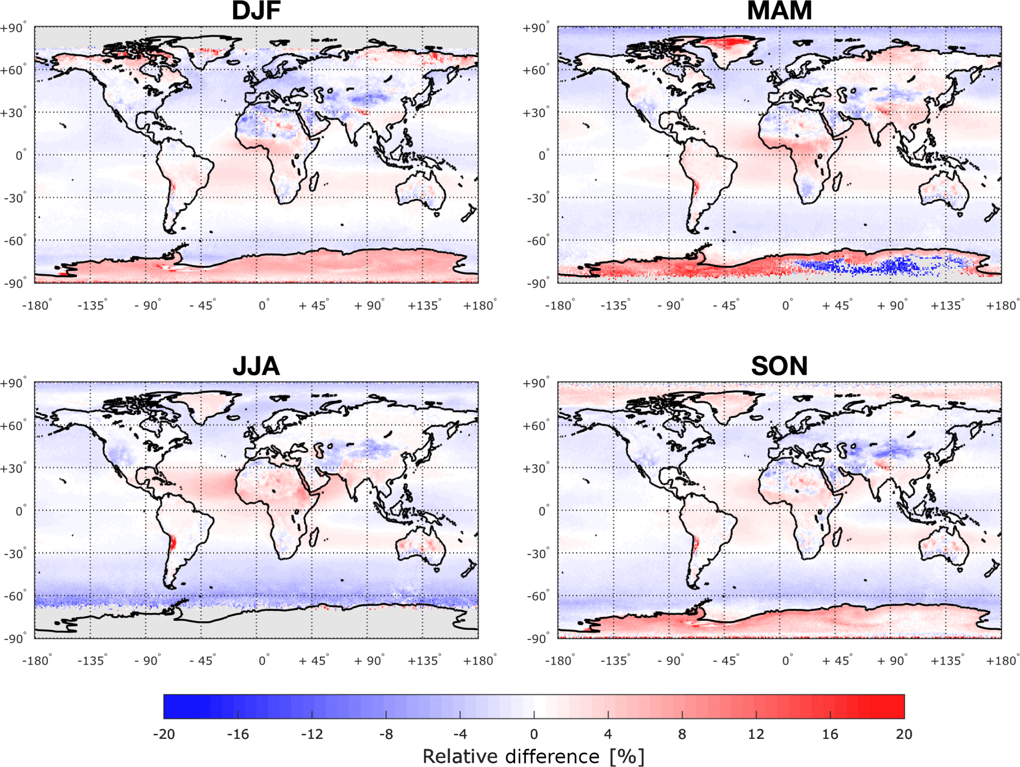
Figure 7Seasonal distribution of the relative differences (in percent) between IASI-A and GOME-2A total ozone column products for the 2008–2017 period. The relative difference is calculated as 100× (IASI-A − GOME-2A) ∕ GOME-2A. DJF represents December–January–February, MAM represents March–April–May, JJA represents June–July–August and SON represents September–October–November.
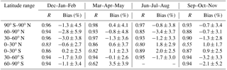
Table 2Summary of the correlation (R), the mean bias and the standard deviation values of IASI-A and GOME-2A TOC products computed from daily gridded data, for each season of the 2008–2017 period. The bias and the 1σ standard deviation are given in percent. The correlation coefficients lower than 0.85 are indicated in italics.
The interannual variability of IASI-A TOCs and TROPO O3 columns is illustrated in Fig. 5. The highest TOC occurs in the northern mid- and high- latitudes during springtime while the lowest TOC values (<200 DU) occur in the southern high latitudes from September to November. The lowest TROPO O3 occurs south of 70∘ S as well as in the tropics (values less than 15 DU), whereas monthly mean TROPO O3 values occur in the northern midlatitudes during summer, and are mainly caused by stratosphere–troposphere exchange processes in spring–summer coupled with O3 production from pollution events in summer.
5.1 Comparison with GOME-2 TOCs
Figure 6 illustrates the 1∘ zonal monthly relative differences between IASI-A and GOME-2A TOCs (computed from daily data) for the period from 2008 to 2017 and their associated standard deviation. Good agreement is observed between both TOC products, with the lowest differences found in the midlatitudes and tropics and the largest differences found in the polar regions, especially over Antarctica (differences larger than 20 %). In the tropics the differences are mostly positive, while they are negative in the midlatitudes.
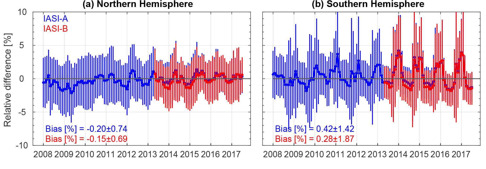
Figure 8Monthly relative differences (in percent) between IASI-A (blue) and IASI-B (red) against GOME-2A total ozone column products as a function of time for the 2008–2017 period for the Northern Hemisphere (a) and the Southern Hemisphere (b). The 1σ standard deviation of the relative differences is also displayed (vertical bars). For each grid cell, a relative difference is calculated as 100× (IASI − GOME-2) ∕ GOME-2 [%]. All the relative differences in each hemisphere are then monthly averaged. Comparison statistics including the mean bias and its 1σ standard deviation in percent for the 2008–2017 period (IASI-A) and the 2013–2017 period (IASI-B) are indicated on each panel.
Figure 7 shows the seasonal distributions of relative differences between IASI-A and GOME-2A TOCs, computed from daily gridded data for the 2008–2017 period (see Table 2 for the associated statistics). The smallest differences are found in the northern midlatitudes during summer (June–July–August) where the IASI sensitivity is the highest, while the largest differences are found over the cold surfaces of Antarctica and Greenland where the IASI sensitivity is the lowest, especially during the March–April–May (MAM) season (3.5 % over Antarctica). The detailed analysis undertaken for different latitude bands given in Table 2 shows that the highest correlation coefficients are found in the midlatitudes and the northern high latitudes, with values higher than 0.93. Lower correlation is found between IASI-A and GOME-2A TOCs in the southern high latitudes during MAM (0.62) and in the tropics during SON (September–October–November) (0.55). However, during the O3 hole season, a high correlation of 0.94 is found in the southern polar region, and IASI-A TOCs are negatively biased (∼2 %). This suggests that IASI-A TOC overestimates the extent of O3 depletion (i.e., underestimates the TOCs in the ozone hole) with respect to GOME-2A TOC. Figure 8 illustrates the time series of the monthly mean relative difference between IASI-A and IASI-B against GOME-2A TOCs along with the standard deviation for the Northern Hemisphere (NH) and the Southern Hemisphere (SH). There is a pronounced seasonality in the difference between IASI-A and IASI-B against GOME-2A TOCs in the SH, with the largest differences being found during austral summer (up to 4 %) and the lowest differences during the austral winter. Compared to GOME-2A data, IASI-A (IASI-B) TOC shows less O3 in the NH by 0.20±0.74 % (0.15±0.69 %) and more O3 in the SH by 0.42±1.42 % (0.28±1.87 %); these differences are within the total retrieval error bars of the two products. Globally, the IASI-A (IASI-B) TOC product is slightly higher than the GOME-2A TOC product, with a global mean bias of 0.3±0.8 % (0.4±0.8 %). It is worth noting that the previous IASI TOC product (v20140922) was in disagreement by more than 5 % (Boynard et al., 2016). The global mean bias is now within the total errors of GOME-2, (estimated to 3 %–7 %; Valks et al., 2017) and IASI, which demonstrates the good consistency between the IASI and GOME-2 TOC products.
Despite the global improvement of ∼5 % with the new IASI TOC product with respect to the previous IASI TOC product (v20140922), large discrepancies are still observed at high latitudes and are partly explained by the following:
- i.
The low spectral signal to noise ratio due to very low surface temperature in high-latitude regions lead to limited information content in the IASI observations in these areas.
- ii.
A misrepresentation of the wavenumber-dependent surface emissivity, which is a critical input parameter to describe the surface, especially above continental surfaces (Hurtmans et al., 2012), can occur in high-latitude regions. FORLI uses the emissivity climatology built by Zhou et al. (2011) providing weekly emissivity values on a latitude/longitude grid for all 8461 IASI spectral channels. However, Zhou et al. (2011) climatology can have missing values. In such cases, the MODIS climatology built by Wan (2006), which provides values for only 12 channels in the IASI spectral range is used instead. Furthermore, in cases where there is no correspondence between the IASI pixel and either climatologies, the reference emissivity used for the Zhou climatology (Zhou et al., 2011) is used, which can significantly impact the retrievals. This is particularly true in arid or semi-arid regions where variations in emissivity are large both on spectral and spatial scales (Capelle et al., 2012) and also in ice regions as the reference emissivity does not necessarily reflect the actual snow or sea ice coverage.
- iii.
The temperature profiles used in FORLI-O3 are less reliable at high latitudes and over elevated terrain (August et al., 2012). As shown in Boynard et al. (2009), the errors introduced by the uncertainties of 2 K on the temperature profile can reach up to 10 % of total error on the retrieved vertical profile, with the error due to the temperature uncertainty on the TOCs being much lower. Errors on thermal contrast can also have an impact on the retrievals.
- iv.
The errors associated with TOC retrievals in the UV–vis spectral range increase at high solar zenith angles in high-latitude regions, mostly due to the larger sensitivity of the retrieval to the a priori O3 profile shape (Lerot et al., 2014).
In the section below, a detailed analysis of the larger bias found in the Antarctic region is undertaken for individual ground-based Brewer and Dobson stations to try to understand this larger bias (see next section).

Figure 9Latitudinal variability of the relative difference (in percent) between IASI-A (blue) and IASI-B (red) against collocated Dobson (a) and Brewer (b) TOC data given in bins of 10∘. Only the common collocations between the two satellites are shown (May 2013–July 2017 period). The 1σ standard deviation of the relative differences is also displayed (vertical bars). The relative difference is calculated as 100× (IASI − GB) ∕ GB [%].
Due to several years of GOME-2 instrumental degradation (Dikty et al., 2011), the stability of IASI-A and IASI-B is not assessed from comparison with GOME-2A. It will be explored in the subsections below against the other independent datasets used in this study.

Figure 10Time series of the monthly relative differences (in percent) between IASI-A (blue) and IASI-B (red) against collocated ground-based (GB) TOC for the Northern Hemisphere for the Dobson (a) and Brewer (b) networks. For each daily GB measurement, a relative difference is calculated as 100× (IASI − GB) ∕ GB [%]. All the relative differences are then monthly averaged. For the period from May 2013 onwards, only the common collocations between IASI-A and IASI-B are shown. The 1σ standard deviation of the average is also displayed (vertical bars). Comparison statistics including the mean bias and its 1σ standard deviation in percent for the 2008–2017 period (IASI-A) and 2013–2017 period (IASI-B) are indicated on each panel. The decadal drift, its 2σ standard deviation (in percent) and the P value for the IASI-A time series are also indicated on each panel.
5.2 Comparison with Brewer–Dobson TOCs
Figure 9 shows the dependency of the relative differences of IASI-A and IASI-B against GB measurements on latitude for the period from May 2013 to July 2017. For each daily ground-based measurement a relative difference is calculated as 100× (IASI − GB) ∕ GB [%]. All relative differences are then separated into latitudinal bins of 10∘ and the mean is calculated. As expected, very similar features can be seen between the IASI-A and IASI-B comparisons, with the Antarctic (80–90∘ S latitude band) being largely overestimated (∼20 %) and the northern middle latitudes driving the mean comparisons to around the 0 % to 2 % level. As shown by the IASI-to-Dobson comparison (Fig. 9a), the dependency on latitude is less visible for the NH due to the high number of collocations which render the latitudinal means more representative than those of the SH. The comparisons with Dobson measurements show differences between 0 and 2.5 % for the entire NH (except in the 70–80∘ N belt where the difference reaches 3.5 % for IASI-A) and for latitudes ranging between 0 and 40∘ S. South of 40∘ S, the differences range between 2 % and 4 %, which is partially attributed to the small number of stations, the limited sensitivity in this region (especially for latitudes lower than 60∘ S) and the larger TOC variability within the southern polar vortex (Garane et al., 2018, this issue; Verhoelst et al., 2015). The comparison with Brewer measurements show a similar picture for the NH. Note that there are a few Brewer stations in the SH, but they are not evenly distributed (all of them are located on the Antarctic) so their measurements are not used. Figure 9 also clearly displays the larger differences for the 20–30∘ N latitude band (more visible for the comparison with Brewer measurements), where some desert stations, like Tamanrasset, Algeria and Aswan, Egypt (see further discussion in the next paragraph) are located; this suggests that the IASI quality flag established to filter the high values linked with emissivity-related issues (based on the ratio of the surface–6 km column relative to the TOC) is rather loose. Nevertheless the overall comparison with Dobson and Brewer TOCs shows that the new IASI TOC product is improved by 4 % in comparison with the previous IASI TOC product (v20140922; see Boynard et al., 2016) and is within IASI and GB TOC total error bars.
To further examine the large discrepancies mentioned above, we analyzed the results obtained for individual stations located in Antarctic and desert regions in more detail. The stations located near desert areas show a diverging behavior with positive (Tamanrasset, Algeria) and negative (Aswan, Egypt and Springbok, South Africa) biases of +7 % to +8 % and −5 % to −4 %, respectively. Over Antarctica, four stations were examined. The bias was found to be extremely high (∼20 %) for Amundsen-Scott, which is located at 90∘ S and at an altitude of 3 km, and less (but still positive) for the other three stations: Halley Bay, Syowa and Arrival Heights (1.2 %–3.8 %), which are located on the Antarctic Ice Sheet. The comparison of GOME-2A with ground-based TOCs at Amundsen-Scott shows a very small bias of 1 %–2 %, indicating that there is no obvious issue with the ground-based measurements. Furthermore, the scatterplot for that particular station (compared to either Dobson or Brewer; plot not shown) shows that IASI-A has a much higher variability than the GB TOC values. This issue needs to be further explored by investigating, for instance, the impact of potential surface emissivity discrepancies on the retrievals over some regions of Antarctica and over deserts. Additional quality filters, e.g., on ice surface emissivity issues, could also be considered.
Figure 10 shows the time series of the monthly relative differences between IASI-A, IASI-B and GB TOC over the corresponding IASI measurement period for the NH only. For each GB measurement, a daily relative difference is calculated. All the relative differences are then averaged per month. Each month includes more than 180 IASI GB pairs. As for GOME-2, we see an obvious seasonal variability in the differences, especially for the Dobson measurements: the smallest differences appear in summer and the largest differences in winter. The larger seasonal variability in the Dobson comparisons is explained by the fact that the Dobson measurements strongly depend on the stratospheric effective temperature (Koukouli et al., 2016). We also see a similar but less pronounced seasonal effect in the Brewer comparison. According to Garane et al. (2018, this issue) and references therein, even though Dobson and Brewer spectrometers basically follow the same principles of operation, TOC measurements from the two types of instruments show differences in the range of ±0.6 %; this is due to the use of different wavelengths in their respective TOC algorithms and the different temperature dependencies of the ozone absorption coefficients. However, it is worth noting that these differences between Brewer and Dobson TOCs are lower than their total uncertainty (∼1 %). The mean difference for the NH is lower than 1.1 % for both Dobson and Brewer comparisons to the IASI observations.
According to the user requirements given in the “User Requirement Document” of the Ozone_cci project (van Weele et al., 2016), the stability of the ozone measurements must be between 1 % and 3 % decade−1. To assess the long-term stability of the IASI-A TOC products, which is essential for trend studies, we calculate the IASI-A TOC decadal drift from the monthly relative differences between IASI-A and GB TOC over the period from 2008 to 2017 (see Fig. 10). The drift is considered statistically significant if its P value is lower than 0.05 and the drift value is higher than its 2σ standard deviation. For the Dobson comparison, the TOC relative differences exhibit insignificant drift of 0.68±0.69 % decade−1. For the Brewer comparison, a <3 % positive drift of 1.38±0.50 % decade−1 is found. When comparing against Brewer and Dobson measurements, the results show that the IASI-A TOC products are stable; thus, they are reliable for trend studies, as expected from the excellent stability in the Level 1 data (Buffet et al., 2016).
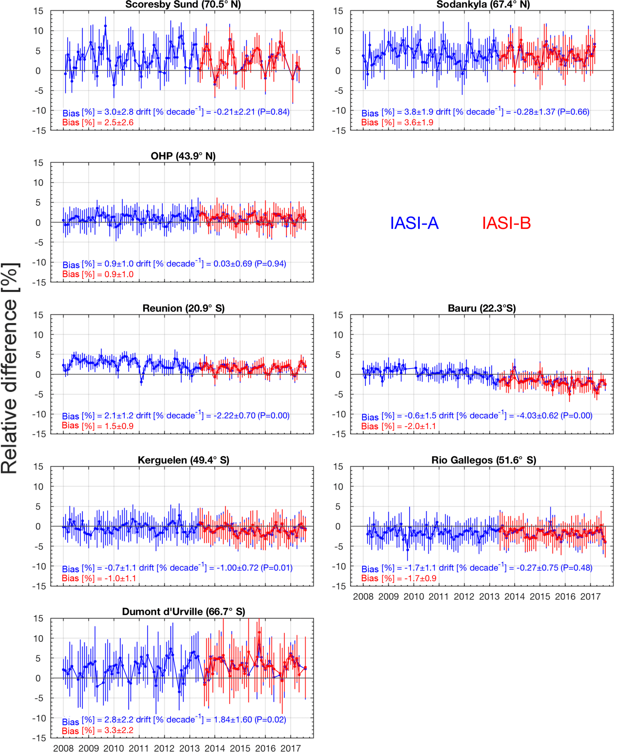
Figure 11Time series of the monthly relative differences (in percent) between IASI-A (blue) and IASI-B (red) against collocated SAOZ TOC measurements for eight stations from north to south. For each daily SAOZ measurement, a relative difference is calculated as 100× (IASI − SAOZ) ∕ SAOZ [%]. All the relative differences are then monthly averaged. For the period from May 2013 onwards, only the common collocations between IASI-A and IASI-B are shown. The standard deviation of the average is also displayed (vertical bars). Comparison statistics including the mean bias and its 1σ standard deviation (in percent) for the period from 2008 to 2017 (IASI-A) and 2013 to 2017 (IASI-B) are indicated on each panel. The decadal drift, its 2σ standard deviation (in percent) and the P value for the IASI-A time series are also indicated on each panel.
5.3 Comparison with SAOZ TOCs
Figure 11 shows the temporal variation of the daytime monthly mean relative differences between IASI-A and IASI-B against SAOZ TOCs for the eight SAOZ stations for the period from 2008 to 2017. For each daily SAOZ measurement, a relative difference is calculated as 100× (IASI − SAOZ) ∕ SAOZ [%]. All the relative differences are then monthly averaged. First, we clearly see the systematic seasonality in the differences, with increasing amplitude with latitude. Compared to SAOZ, the IASI-A and IASI-B TOCs are biased by 0.5 %–2 % (∼1 % monthly mean averaged standard deviation) in the tropics and midlatitudes, and are biased high to about 4±3 % inside the polar circle. The results are consistent with those found for the comparison with GOME-2A along with Brewer and Dobson measurements (see Sect. 5.1 and 5.2, respectively). An improvement of 3 %–4 % is found when compared to the previous IASI product (v20140922).
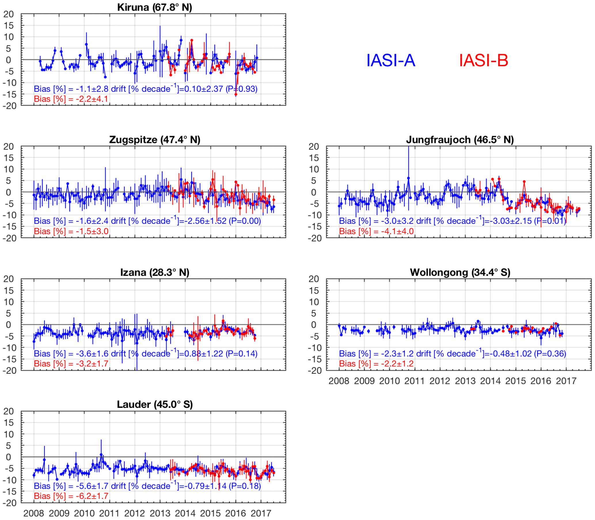
Figure 12Time series of the monthly relative differences (in percent) between IASI-A (blue) and IASI-B (red) against collocated FTIR TOC measurements for six stations from north to south over the period from 2008 to July 2017. For each daily FTIR measurement, a relative difference is calculated as 100× (IASI − FTIR) ∕ FTIR [%]. All the relative differences are then monthly averaged. The standard deviation of the average is also displayed (vertical bars). Comparison statistics including the mean bias and its 1σ standard deviation (in percent) for the period from 2008 to 2017 (IASI-A) and 2013 to 2017 (IASI-B) are indicated on each panel. The decadal drift, its 2σ standard deviation (in percent) and the P value for the IASI-A time series are also indicated on each panel.
The IASI-A and SAOZ TOC relative differences show small or insignificant negative decadal drifts ranging between % (OHP) and % (Reunion). Bauru station is an exception to these drifts due to a SAOZ retrieval issue still under investigation. The good quality of the IASI-A TOC temporal stability satisfies the 1 %–3 % decade−1 Ozone_cci requirements for the long-term stability for total ozone measurements well (Van Weele et al., 2016), which again shows that the current IASI-A TOC products are homogeneous and reliable for trend studies.
5.4 Comparison with FTIR TOCs and partial ozone columns
Figure 12 shows the temporal variation of the monthly mean relative differences between IASI-A and IASI-B against FTIR TOCs convolved with the IASI averaging kernels according to Eq. (2) for the six FTIR stations (see Table 1 and Fig. 2 for their location) for the period from 2008 to 2017. Compared to FTIR, the IASI-A and IASI-B TOCs are negatively biased by 0.8 %–6.2 % with the largest biases of −4.1 % and −6.2 % at Jungfraujoch and Lauder, respectively. At Lauder, mean biases of 5.7±5.4 % and 0.6±6.4 % are found for FTIR and IASI against Dobson TOCs, respectively, suggesting that the FTIR data might be biased high at that station. However, 4 % of this bias between FTIR and Dobson is likely due to the known inconsistency between IR and UV cross sections (Gratien et al., 2010) (note that the bias is calculated as [100× (FTIR − DOBSON) ∕ DOBSON] or [100× (IASI − DOBSON) ∕ DOBSON]). It can be noted that the biases between FTIR and IASI-A, and SAOZ and IASI-A for stations that are located close to one another with regards to latitude are very consistent if one takes this spectroscopic bias into account (i.e., UV at Sodankyla lower than IASI-A by 3.9 %, FTIR at Kiruna higher by 1.1 %; UV at OHP lower than IASI-A by 1.0 %, FTIR at Jungfraujoch higher by 3 %; UV at Kerguelen higher than IASI-A by 0.9 %, and FTIR at Lauder higher by 6.2 %).
At Zugspitze and more particularly at Jungfraujoch, two jumps are visible in 2010 and 2014, with larger biases before 2011 and after 2014 with respect to the period in between. It is worth noting that these two jumps seem to coincide with changes in IASI Level 2 temperature (in September 2010 and September 2014). The analysis of surface temperatures used in both IASI (EUMETSAT) and FTIR (NCEP) retrievals (IASI Level 2 EUMETSAT and NCEP, respectively) shows that the differences between EUMETSAT and NCEP can reach up to 20 K for the surface temperature and vary between −10 and 10 K along the temperature vertical profile at both Jungfraujoch and Zugspitze. However, at the other stations the differences are much lower (less than 5 K). This suggests that IASI Level 2 EUMETSAT temperatures are less reliable above elevated areas. However a more in-depth analysis is needed (and is currently in progress) in order to understand the exact origin of the jumps found in the differences between IASI and FTIR TOCs at these stations.
The dominant systematic uncertainty in FTIR O3 retrievals is due to the spectroscopic parameters (García et al., 2012). The IASI retrieval algorithm uses HITRAN 2012 and the FTIR retrieval algorithm uses HITRAN 2008, although no differences were found in either O3 absorption band (Boynard et al., 2016). We do not expect a significant bias between the IASI and FTIR total columns due to ozone spectroscopy, as both retrieval algorithms use the same ozone spectroscopic parameters and the same fitting spectral range. Except at Lauder and Jungfraujoch, the mean biases between IASI and FTIR TOCs are relatively low and within total errors of FTIR (e.g., García et al., 2012) and IASI, which once more reenforces the good quality of IASI TOC data.
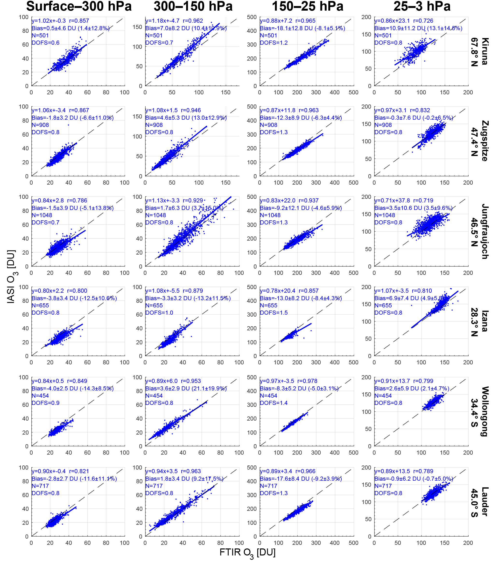
Figure 13Scatterplots of IASI-A against smoothed FTIR O3 partial columns at the six FTIR stations for the period from 2008 to 2017. Comparison statistics including the linear regression, the mean bias, the 1σ standard deviation in both Dobson units (DU) and percent (%), the number of collocations and the mean DOFS for each partial column are shown on each panel.
At all stations except for Jungfraujoch and Zugspitze, the IASI-A and FTIR TOC monthly relative differences show insignificant drifts of less than 0.9 % decade−1 (see Fig. 12 and Table 2), which is within the 1 %–3 % decade−1 Ozone_cci requirements for the long-term stability of total ozone measurements (Van Weele et al., 2016). This demonstrates that the current IASI-A TOC products are homogeneous and reliable for trend studies. The significant negative drifts found at Jungfraujoch and Zugspitze, are explained by the bias drop observed from 2014, which is discussed above.
As FTIR data also provide up to four independent pieces of information in the vertical ozone profile, we assess four IASI partial ozone columns characterized by a DOFS of ∼1 (surface–300, 300–150, 150–25 and 25–3 hPa), which should make such assessment meaningful. The comparisons of the four partial ozone columns between IASI-A and FTIR performed for the period from 2008 to 2017 are presented in Fig. 13. The correlation coefficients between FTIR and IASI-A partial columns are good to excellent (from 0.72 to 0.98), with the highest correlations found in the UTLS and LMS.
For all stations except Kiruna, the IASI tropospheric column is negatively biased by 5 %–14 %. The comparison for the UTLS O3 columns shows that the IASI-A O3 product is positively biased at all stations (except Izaña), with the highest bias found at Wollongong (21.1±19.9 %) and the lowest bias found at Jungfraujoch (3.7±15.0 %). The standard deviation is highest in the UTLS at Izaña and Lauder, which is due to strong O3 variability and a large total retrieval error in this region as shown in Wespes et al. (2016). Indeed, Fig. 4b in Wespes et al. (2016) demonstrated that the estimated total retrieval error of vertical ozone profiles from IASI in tropical regions are larger than in middle latitudes, which suggests that this would also be the case for the ozone column. It should be noted that IASI is positively biased in the UTLS region, as reported in previous studies comparing IASI to ozonesonde data (e.g., Boynard et al., 2016; Dufour et al., 2012; Gazeaux et al., 2013). Although Dufour et al. (2012) attempted to give some explanations for this particular feature, the exact reason for this overestimation is still not clear. One reason may be the use of inadequate a priori information. Note that FORLI only uses one single a priori profile (Hurtmans et al., 2012): the global mean profile of the McPeters/Labow/Logan climatology (McPeters et al., 2007). As shown by Bak et al. (2013), using tropopause-based ozone profile climatology can significantly improve the a priori profile. However, using dynamical a priori information makes the comparison on a global scale less straightforward as a different a priori profile is used at each IASI pixel. The best correlation coefficients and smallest standard deviations (in percent) between IASI-A and FTIR data are found for the LMS column. The small standard deviations in the LMS comparisons allow the detection of consistent IASI-A negative biases at all stations (5 %–9 %). This consistent negative bias in the LMS, where the ozone partial column contributes the most to the total column, is reflected in the observed negative bias in TOC discussed above. These better correlation coefficients and standard deviations in the LMS are due to the better IASI sensitivity to this column (mean DOFS ∼1.2–1.5 as indicated in Fig. 13) compared to the other partial columns. The smallest biases between FTIR and IASI-A columns are found in the MS column ( %), except at Kiruna where the bias reaches 13 %. This higher bias at Kiruna might be due to a bad collocation of sounded air masses which can be different in or out of polar vortex conditions for the two instruments. The FTIR instrument sounds the atmosphere along the sun–instrument line of sight; therefore, the sounded air masses in this higher partial column and for high solar zenith angles measurements might be located a fair distance from the station itself (few hundreds kilometers). Thus, collocation with the satellite, which would take the FTIR line of sight into account, would improve the comparisons.
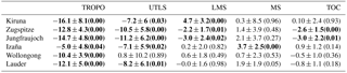
Table 3IASI-A decadal drifts and their 2σ standard deviation (in percent) calculated from the monthly relative differences between IASI and the FTIR data over the period from 2008 to 2017 for the TOC and different partial ozone columns: surface–300 hPa (TROPO), 300–150 hPa (UTLS), 150–25 hPa (LMS) and 25–3 hPa (MS). The P value is indicated in parentheses. A P value lower than 0.05 indicates a significant drift; drifts indicated in bold are significant.
Similar results are found for the comparison of IASI-B with FTIR partial ozone columns over the period from May 2013 to 2017 (not shown).
The stability of the IASI-A partial ozone columns is also assessed based on the time series of monthly relative differences between IASI-A and FTIR data over the period from 2008 to July 2017. Table 3 gives the decadal drift values along with their 2σ standard deviations in percent per decade ( % decade−1) as well as the P value. As a reminder, the drift is considered significant if the drift value is higher than its 2σ standard deviation. For the TROPO column, we clearly see a significant negative drift at all stations ranging from % decade−1 (Izaña) to % decade−1 (Kiruna). Smaller or insignificant drifts are found in the UTLS and LMS. Regarding the MS, insignificant positive drifts are found, except at Izaña where a positive drift is found (3.7±2.5 % decade−1). As a consequence, the stability of the IASI-A partial O3 columns compared to the six FTIR GB measurements that cover the IASI measurement period and that are characterized by limited vertical sensitivity cannot be confirmed.

Figure 14Scatterplots of collocated IASI-A and smoothed ozonesonde O3 partial columns for six latitude bands for the period from 2008 to 2017. Comparison statistics including the linear regression, the mean bias, the 1σ standard deviation in both Dobson units (DU) and percent (%), the number of collocations and the mean DOFS for each partial column are shown on each panel.
The stability of the IASI-A partial O3 columns was analyzed in detail by comparisons with ozonesonde measurements that provide numerous highly resolved vertical O3 profiles. This comparison is outlined in the following section.
5.5 Comparison with ozonesonde partial ozone columns
A statistical comparison of IASI-A and IASI-B against sonde partial ozone columns at 56 stations (see Fig. 2) was performed, which gathered approximatively 2000 ozonesonde profiles during a period extending from May 2013 to July 2017 and 11 600 ozonesonde profiles over the whole IASI measurement period (2008–2017). In order to assess the latitudinal variability of IASI O3 retrieval performance, the comparison was performed for six 30∘ latitude bands representative of the northern high latitudes (60–90∘ N), northern midlatitudes (30–60∘ N), northern tropics (0–30∘ N), southern tropics (0–30∘ S), southern midlatitudes (30–60∘ S) and southern high latitudes (60–90∘ S).
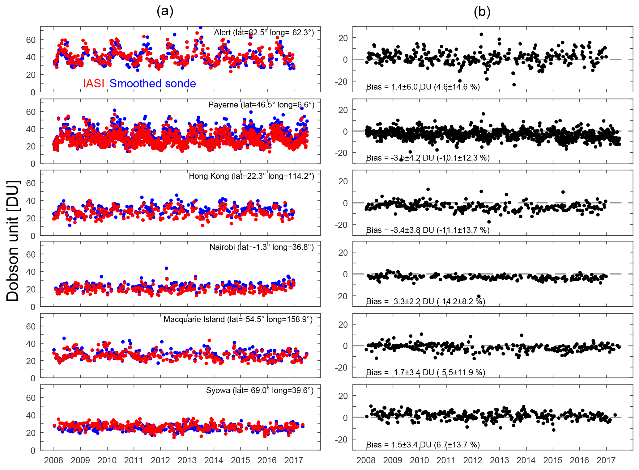
Figure 15(a) Time series of daily IASI-A (in red) and smoothed ozonesonde (in blue) TROPO O3 columns in Dobson units (DU) for six stations representative of different latitude bands for the period from 2008 to 2017. (b) The associated relative differences (in percent), calculated as 100× (IASI − SONDE) ∕ SONDE, including the mean bias and the 1σ standard deviation.
Figure 14 shows the comparison of IASI-A against smoothed ozonesonde for four partial columns for each of the six latitude bands during the 2008–2017 period. For the TROPO O3 columns (Fig. 14, first column), the mean biases and standard deviation are within 20 %. IASI-A underestimates the O3 abundance in the tropics and midlatitudes (by ∼16 %–19 % and ∼6 %–11 %, respectively) and overestimates the O3 abundance at high latitudes (by 4 %–5 %), compared with ozonesonde data. The correlation coefficients range from 0.8 to 0.9 in the tropics to 0.7 to 0.8 at middle latitudes, and from 0.5 to 0.8 at high latitudes. The linear regression slopes are in the range of 0.6–0.8, with lower values found at high latitudes due to the reduced retrieval sensitivity in the lower troposphere. It is worth noting that a lower correlation coefficient is found for the southern midlatitudes, which is likely due to the lower amount of data in comparison with the other latitude bands. The comparison for the UTLS O3 columns (Fig. 14, second column) shows that IASI-A O3 products overestimate the O3 abundance irrespective of latitude, with the highest biases found at high latitudes (30 %–42 %) and the lowest biases found at midlatitudes (∼11 %–19 %). The standard deviation is highest in the UTLS in all latitude bands (compared to the other partial columns) due to the strong O3 variability and the large total retrieval error, as shown in Wespes et al. (2016). The linear regression slopes are close to 1 in the polar and midlatitude regions but are around 0.4 in the tropics, which is closely related to the small amount of O3 in the tropical UTLS. A positive bias from IASI-A O3 products is also found for the LMS (Fig. 14, third column) and MS (Fig. 14, fourth column) columns (except at high latitudes for the latter). The correlation coefficients range between 0.6 (tropics and high latitudes) and 0.8 (midlatitudes) for the LMS column while they are much lower for the MS column, which is explained by the low DOFS values ranging between 0.4 and 0.6 (as indicated on the scatterplots). Note that the DOFS for the MS columns are lower than those calculated in Fig. 13 because they do not correspond to the full MS column calculated from IASI (25–3 hPa, i.e., ∼25–40 km); instead the DOFS correspond to the MS columns truncated to match the maximum altitude (30–35 km) of the sonde measurements. The mean DOFS is generally in the range of 0.6–1.4 for the TROPO, UTLS and LMS columns, with the larger DOFS being found for the LMS column. Similar results are found for the comparison of IASI-A and IASI-B with sonde partial ozone columns over the common period from May 2013 to 2017, except for the MS in the 60–90∘ S latitude band (not shown). In comparison with the previous IASI partial ozone column products reported in Boynard et al. (2016), the new IASI ozone product is significantly improved in the MS (by 8 %–12 %) for the midlatitudes and tropics. The improvement is less significant for the LMS except in Antarctic where an improvement of 6 % is found. As for the TROPO and UTLS columns, no or slight improvement (<2 %) is found, and the agreement between IASI and sonde data is even worse than for the previous IASI ozone product, especially for the southern tropical TROPO column (by 7 %) and the UTLS column (by 10 %–18 %).
Figure 15 illustrates a sample time series of daily IASI-A and smoothed ozonesondes TROPO O3 columns along with the corresponding differences for six ozonesonde stations representative of different latitude bands over the period from 2008 to 2017. The comparison is good for all latitudes, with IASI-A O3 products underestimating the TROPO O3 abundance in the midlatitudes and tropics by ∼1.7–3.5 DU (5.5 %–10.1 %) and overestimating the TROPO O3 abundance in the high latitudes by ∼1.5 DU (5 %–7 %). This result is generalized in Fig. 2, which shows the mean and standard deviation of the differences in DU between IASI-A and smoothed ozonesonde TROPO O3 columns for each ozonesonde station used in the present work over the period from 2008 to 2017. Overall, the IASI-A TROPO O3 product exhibits good agreement with ozonesonde data at most of the stations, with a mean relative difference and standard deviation within 6 DU. An interesting feature seen in Fig. 2 is that the mean and standard deviation of the differences of TROPO O3 columns between IASI-A and smoothed FTIR is lower than those between the IASI-A and sonde TROPO O3 columns.
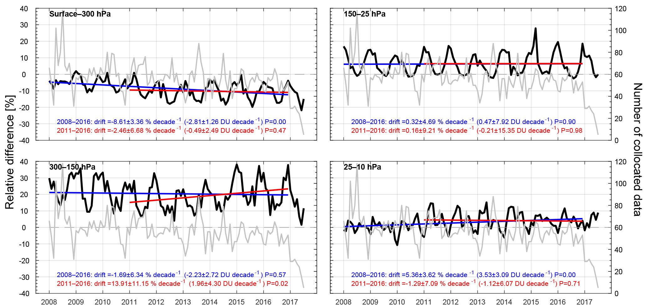
Figure 16Time series of the monthly mean relative differences between IASI-A and ozonesonde O3 measurements for different partial columns for the period from 2008 to 2017 for the Northern Hemisphere. The number of collocated data is also displayed in gray. The decadal drift, its 2σ standard deviation in percent and the P value are indicated on each panel for two periods: 2008–2016 (blue) and 2011–2016 (red).
The long-term stability of the IASI-A partial O3 column vs. ozonesonde measurements is assessed in Figure 16, which presents the monthly relative differences between IASI-A and ozonesonde for the TROPO, UTLS, LMS and MS O3 partial columns for a total of 18 ozonesonde stations in the NH that cover 8 years or longer (from 2008 to 2017). With more than 30 IASI–sonde pairs per month, the NH presents sufficient collocated data to carry out a good statistical drift analysis unlike the SH (only eight ozonesonde stations). For each ozonesonde measurement, a daily relative difference is calculated. All the relative differences are then monthly averaged. A main feature that arises from this figure is the pronounced seasonality in the differences between IASI-A and sonde O3 for the UTLS and LMS column, with the lowest differences found in summer and the highest differences found in winter. We also see a small but apparent seasonality in the differences for the TROPO O3 column: the IASI TROPO O3 column appears less biased with respect to the ozonesondes during winter. This reflects the low sensitivity of IASI associated with low brightness temperature in the troposphere, and in such situations the IASI retrieval mostly provides the a priori information (see Eq. 2). The differences in the TROPO O3 column are better than −10 % during the period from 2008 to 2010 and decrease up to −20 % from 2011. This feature is also visible for the MS column: the difference baseline is around the 0 % level between 2008 and 2010 but near the 4 % level from 2011.
The linear trends of the monthly mean ozone biases for each partial column are plotted in Fig. 16 for the period from 2008 to 2016 (blue line). Note that 2017 is not included in the drift calculation because of the lower number of collocated data for that year. Based on the drift value with the 2σ standard deviation and the P value (indicated on each plot), the derived drifts are insignificant for the UTLS and LMS but are statistically significant for the TROPO and MS columns ( % decade−1 and % decade−1, respectively). This is in agreement with Keppens et al. (2018, this issue) who applied a different method based on the bootstrapping technique (Hubert et al., 2016). Note that for the TROPO column, the drift calculated for each individual station ranges between −16 % decade−1 and −5 % decade−1, which is the same order of magnitude as those found in the IASI-A-to-FTIR TROPO comparison. If we limit the time period to 2011–2016, a statistically significant drift is no longer found for the TROPO and MS (P value > 0.47), as expected from the excellent stability in the Level 1 product (Buffet et al., 2016). However, since this difference in the drift values might only be due to the short time periods considered here associated with the high variability in the TROPO O3 differences, a few more years are needed to confirm the observed negative drifts and evaluate them over longer periods.
In this study, we assessed the quality of IASI-A and IASI-B O3 products (total and partial columns) retrieved with the FORLI v20151001 software for 9 years (2008–2017) through an extensive intercomparison and validation exercise using independent observations (satellite, ground-based and ozonesonde). Compared to the previous version of FORLI-O3 (v20140922), several improvements were introduced in FORLI-O3 v20151001, including absorbance look-up tables recalculated to cover a larger spectral range using the 2012 HITRAN spectroscopic database (Rothman et al., 2013), with additional numerical corrections. This leads to a change of ∼4 % in the total ozone column (TOC) product, which is mainly associated with a decrease in the retrieved O3 concentration in the middle stratosphere (above 30 hPa/25 km). The IASI O3 products processed with FORLI v20151001 are part of the ESA Ozone_cci and ECMWF C3S projects, which focus on building consolidated climate-relevant ozone datasets as ECVs. Therefore, validating the latest version of the IASI O3 products over a long time period and assessing their stability are necessary for decadal trend studies, model simulation evaluation and data assimilation applications. The main findings of this work can be summarized as follows:
-
The intercomparison between IASI-A and IASI-B TOC products for the period from May 2013 to July 2017 shows that IASI-A and IASI-B TOCs are consistent, with a global difference of less than 0.3 % for both daytime and nighttime measurements and with IASI-A TOCs slightly higher than those of IASI-B. A similar result is found for the TROPO O3 column: a global difference of less than 2.4 % for both daytime and nighttime measurements is found, with the IASI-A TROPO O3 columns being lower than those of IASI-B. Inconsistencies between both instruments were found for a limited period between April and September 2015, which were due to the change in the IASI-A viewing angle that was corrected in September 2015 (Buffet et al., 2016). However, it is worth noting that the impact of the IASI-A instrumental issue is within the TOC and TROPO O3 column retrieval error bars. In cases where only IASI-A data are utilized, the user is free to include or exclude the period from April to October 2015 depending on the focus of the study. The consistency between IASI-A and IASI-B O3 products becomes better after September 2015 (differences less than 0.1 % and 1.4 % for the TOC and TROPO O3 column products, respectively), which is due to the better quality of IASI-A and IASI-B Level 1 data. This improvement in data quality stems from the deactivation of IASI's cube corner compensation device, which was proved to generate micro-vibrations and random errors (Buffet et al., 2016; Jacquette et al., 2016).
-
With respect to GOME-2A data, IASI-A and IASI-B TOCs are in excellent agreement: they are marginally lower in the Northern Hemisphere (by 0.2 %), while they are higher in the Southern Hemisphere (by 0.4 %). There is a pronounced seasonality in the differences in the SH, with the largest differences found during the austral summer (up to 4 %); these large differences are related to the larger differences observed in the southern high latitudes. With respect to Dobson and Brewer data, the IASI-A and IASI-B TOC product overestimates the total O3 abundance by 0.5 %–1.1 % with an obvious seasonal variability in the differences, which is caused by the ground-based measurements (see Sect. 5.2 for a more in-depth explanation). Compared to SAOZ, the IASI-A and IASI-B TOC product is biased by 0.6 %–2 % (∼1 % monthly mean averaged standard deviation) in the tropics and midlatitudes, and this value increases to about 2.5 %–3.8 % inside the polar circles. Finally, good agreement is found between IASI-A and IASI-B against the FTIR TOC product, with IASI underestimating the TOC by 1.1 %–6.2 %. The largest bias is found at Lauder, which is likely due to the FTIR data that might be biased high by 1.5 %–2 % at this station. It can be noted that the bias between FTIR and IASI-A, and SAOZ and IASI-A for stations that are close to one another regarding latitude are very consistent if one takes this spectroscopic bias into account (i.e., UV at Sodankyla is lower than IASI-A by 3.8 %, FTIR at Kiruna is higher by 1.1 %; UV at OHP is lower than IASI-A by 0.9 %, FTIR at Jungfraujoch is higher by 3.0 %; UV at Kerguelen is higher than IASI-A by 0.7 %, and FTIR at Lauder is higher by 5.6 %).
-
The time series of relative differences of IASI-A against UV–vis GB TOCs show insignificant negative drift in the NH (0.68±0.69 % decade−1 and P value = 0.05) and a small negative drift in the SH (1.48±0.53 % decade−1 and P value = 0.00), which satisfies the 1 %–3 % decade−1 Ozone_cci requirements for the stability of ozone measurements. Similar results are found for the IASI-A/FTIR TOC comparison. This demonstrates the long-term stability of the current IASI-A TOC products.
-
The comparison results between IASI-A and IASI-B against smoothed FTIR and ozonesonde partial O3 columns vary with altitude, with the maximum standard deviation observed for the UTLS (20 %–40 %) due to strong ozone variability and larger total retrieval errors (Wespes et al., 2016). Attempted explanations for the larger bias found in the UTLS are given in Dufour et al. (2012), although no clear reason for the larger bias was found. A possible explanation may be the use of inadequate a priori information in that layer. The current version of FORLI uses a single global profile that is the mean of the McPeters/Labow/Logan climatology (McPeters et al., 2007) as an a priori profile. As shown by Bak et al. (2013), using tropopause-based ozone profile climatology can significantly improve the a priori profile. However, using dynamical a priori information makes the comparison on a global scale less straightforward to analyze. This is due to the fact that retrievals at each IASI pixel would be based on different a priori profiles. The IASI-A and IASI-B TROPO O3 products underestimate the O3 abundance in the midlatitudes and the tropics (by 11 %–13 % and 16 %–19 %, respectively) and overestimate the O3 abundance in the high latitudes (by 4 %–5 %).
-
The IASI-A-to-FTIR TROPO O3 column comparison exhibits significant negative drifts ranging between −8 % and −16 % decade−1 over the period from 2008 to 2017 at all stations. A significant negative drift of % decade−1 is also found in the IASI-A to ozonesonde TROPO O3 column comparison for the Northern Hemisphere. The observed negative drifts in the IASI-A TROPO columns might partly explain the apparent disagreement between the ozone tropospheric trends observed by IASI and GOME/OMI in the Tropospheric Ozone Assessment Report (TOAR) (Gaudel et al., 2018). However, further investigation should be carried out since the TROPO columns are not calculated in the same way in the two studies. When considering the period from 2011 to 2016, the drift values for the TROPO column decrease and become statistically insignificant. However, since this difference in the drift values might only be due to the short time periods considered in this study, and associated with the high variability in the TROPO O3 differences, a few more years are needed to confirm the observed negative drifts and evaluate them over longer periods. The observed negative drifts of the IASI-A TROPO O3 product (8 %–16 % decade−1) over the 2008–2017 period might also be taken into consideration when deriving trends from this product and this time period.
-
The IASI-A TOC relative differences against independent measurements showed small or insignificant negative decadal drifts for the period from 2008 to 2017, which indicates that the current IASI-A TOC products are homogeneous and reliable for trend studies. The IASI-A TROPO O3 relative differences against sonde and FTIR data showed significant negative drifts for the period from 2008 to 2017. Therefore, it is recommended for trend studies to wait for the new homogeneous IASI climate time series, which will be reprocessed using the ECMWF ERA5 temperature reanalysis (Hersbach and Dee, 2016) and the reprocessed IASI Level 1 data.
The IASI-A and IASI-B O3 products (total and vertical profiles) starting in October 2007 are generated by the LATMOS and ULB in a near real time mode using FORLI-O3 v20151001. Both IASI-A and IASI-B O3 products retrieved using FORLI-O3 v20151001 are already part of the EUMETSAT's AC SAF Official Validation Monitoring found in lap3.physics.auth.gr/eumetsat/ as part of the operational EUMETSAT services. This O3 retrieval algorithm (FORLI-O3 v20151001) is currently being implemented in the EUMETSAT processing facility under the auspices of the AC SAF project in order to operationally distribute Level 2 IASI O3 data to users through the EUMETCast system in 2018.
The IASI O3 data processed with FORLI-O3 v20151001 can be downloaded from the Aeris portal (http://iasi.aeris-data.fr/O3/; Aeris, 2017). The GOME-2 O3 data are available on the AC SAF website (http://acsaf.org; AC SAF, 2017). The ozonesonde data can be downloaded from the WOUDC database (https://doi.org/10.14287/10000008; WMO/GAW Ozone Monitoring Community, 2017a) and from the NOAA-ESRL database (http://www.esrl.noaa.gov/gmd/dv/ftpdata.html; NOAA, 2017). The Brewer and Dobson soundings can be downloaded from the WOUDC database (https://doi.org/10.14287/10000004; WMO/GAW Ozone Monitoring Community, 2017b). The SAOZ data are available at http://saoz.obs.uvsq.fr (SAOZ, 2017). The FTIR data are available at http://www.ndacc.org (FTIR, 2018).
The authors declare that they have no conflict of interest.
This article is part of the special issue “Quadrennial Ozone Symposium 2016 – Status and trends of atmospheric ozone (ACP/AMT inter-journal SI)”. It is a result of the Quadrennial Ozone Symposium 2016, Edinburgh, United Kingdom, 4–9 September 2016.
IASI is a joint mission of EUMETSAT and the Centre National d'Etudes
Spatiales (CNES, France). The IASI Level 1C data are distributed in near real
time by EUMETSAT through the EUMETCast system distribution. The authors
acknowledge the Aeris data infrastructure (https://www.aeris-data.fr/,
last access: 30 August 2018) for providing access to the IASI Level 1C data
and Level 2 temperature data used in this study. This work was undertaken in
the framework of the EUMETSAT AC SAF project (http://acsaf.org), the
European Space Agency O3 Climate Change Initiative (Ozone_cci,
http://www.esa-ozone-cci.org) and the Copernicus Climate Change (C3S).
The French scientists are grateful to CNES and Centre National de la
Recherche Scientifique (CNRS) for financial support. The research in Belgium
is also funded by the Belgian State Federal Office for Scientific, Technical
and Cultural Affairs and the European Space Agency (ESA Prodex IASI Flow
project). The ozonesonde data used in this study were provided by the World
Ozone and Ultraviolet Data Centre (WOUDC) and the Global Monitoring Division
(GMD) of NOAA's Earth System Research Laboratory and are publicly available
(see http://www.woudc.org and http://www.esrl.noaa.gov/gmd). The
authors thank all those responsible for the WOUDC and GMD measurements and
archives for making the ozonesonde data available. The ground-based total
ozone column data used in this publication were obtained as part of WMO's
Global Atmosphere Watch (GAW) and are publicly available via the WOUDC. We
would like to acknowledge and warmly thank all of the investigators that
provide data to these repositories on a timely basis, as well as the handlers
of these databases for their upkeep and efforts to achieve the guaranteed
quality of the product. The FTIR data used in this publication were obtained
as part of the Network for the Detection of Atmospheric Composition Change
(NDACC) and are publicly available (see http://www.ndacc.org). The
multi-decadal monitoring program of ULiege at the Jungfraujoch station has
been primarily supported by the F.R.S.-FNRS and BELSPO (both in Brussels,
Belgium) and by the GAW-CH programme of MeteoSwiss. The International
Foundation High Altitude Research Stations Jungfraujoch and Gornergrat
(HFSJG, Bern) supported the facilities needed to perform the FTIR
observations. NDACC data from Kiruna were recorded at the Swedish Institute
of Space Physics (IRF) Kiruna. The authors would like to thank Uwe Raffalski
and Peter Völger from IRF Kiruna and Thomas Blumenstock, Frank Hase and
Jochen Gross from KIT Karlsruhe for performing and analyzing the FTIR
measurements at Kiruna. NDACC data from Izaña were recorded at the
Izaña Observatory on Tenerife Island. The authors would like to thank
Omaira Garcia and Eliezer Sepúlveda, AEMet Spain, and Matthias Schneider,
Frank Hase and Thomas Blumenstock from KIT Karlsruhe for performing and
analyzing the FTIR measurements at Izaña. The authors acknowledge the
European Communities, the Région Réunion, CNRS, and Université de
la Réunion for their support and contribution in the construction phase
of the research infrastructure OPAR (Observatoire de la Physique de
l'Atmosphère à la Réunion). OPAR is presently funded by CNRS
(INSU) and Université de la Réunion, and managed by OSU-R
(Observation des sciences de l'Univers à la Réunion, UMS 3365).
Françoise Posny, Thierry Portafaix (LACy – UMR 8105) and
Jean-Marc Metzger (UMS 3365) are also acknowledged for their management,
scientific follow up and technical handling of the SAOZ and ECC observations
at La Réunion.
Edited by: Irina Petropavlovskikh
Reviewed by: three anonymous referees
AC SAF: The AC SAF GOME-2 O3 products, available at: http://acsaf.org, last access: 30 August 2017.
Aeris: The IASI O3 products processed with FORLI-O3 v20151001, available at: http://iasi.aeris-data.fr/O3/, last access: 22 December 2017.
August, T., Klaes, D., Schlüssel, P., Hultberg, T., Crapeau, M., Arriaga, A., O'Carroll, A., Coppens, D., Munro, R., and Calbet, X.: IASI on Metop-A: Operational Level 2 retrievals after five years in orbit, J. Quant. Spectrosc. Ra., 113, 1340–1371, https://doi.org/10.1016/j.jqsrt.2012.02.028, 2012.
Bak, J., Liu, X., Wei, J. C., Pan, L. L., Chance, K., and Kim, J. H.: Improvement of OMI ozone profile retrievals in the upper troposphere and lower stratosphere by the use of a tropopause-based ozone profile climatology, Atmos. Meas. Tech., 6, 2239–2254, https://doi.org/10.5194/amt-6-2239-2013, 2013.
Balis, D., Kroon, M., Koukouli, M. E., Labow, G., Veefkind, J. P., and McPeters, R. D.: Validation of Ozone Monitoring Instrument total ozone column measurements using Brewer and Dobson spectrophotometer ground based observations, J. Geophys. Res., 112, D24S46, https://doi.org/10.1029/2007JD008796, 2007a.
Balis, D., Lambert, J.-C., Van Roozendael, M., Spurr, R., Loyola, D., Livschitz, Y., Valks, P., Amiridis, V., Gerard, P., Granville, J., and Zehner, C.: Ten years of GOME/ERS2 total ozone data the new GOME data processor (GDP) version 4: 2. Ground-based validation and comparisons with TOMS V7/V8, J. Geophys. Res., 112, D07307, https://doi.org/10.1029/2005JD006376, 2007b.
Barret, B., Le Flochmoen, E., Sauvage, B., Pavelin, E., Matricardi, M., and Cammas, J. P.: The detection of post-monsoon tropospheric ozone variability over south Asia using IASI data, Atmos. Chem. Phys., 11, 9533–9548, https://doi.org/10.5194/acp-11-9533-2011, 2011.
Boynard, A., Clerbaux, C., Coheur, P.-F., Hurtmans, D., Turquety, S., George, M., Hadji-Lazaro, J., Keim, C., and Meyer-Arnek, J.: Measurements of total and tropospheric ozone from IASI: comparison with correlative satellite, ground-based and ozonesonde observations, Atmos. Chem. Phys., 9, 6255–6271, https://doi.org/10.5194/acp-9-6255-2009, 2009.
Boynard, A., Hurtmans, D., Koukouli, M. E., Goutail, F., Bureau, J., Safieddine, S., Lerot, C., Hadji-Lazaro, J., Wespes, C., Pommereau, J.-P., Pazmino, A., Zyrichidou, I., Balis, D., Barbe, A., Mikhailenko, S. N., Loyola, D., Valks, P., Van Roozendael, M., Coheur, P.-F., and Clerbaux, C.: Seven years of IASI ozone retrievals from FORLI: validation with independent total column and vertical profile measurements, Atmos. Meas. Tech., 9, 4327–4353, https://doi.org/10.5194/amt-9-4327-2016, 2016.
Brunekreef, B. and Holgate, S. T.: Air pollution and health, Lancet, 360, 1233–1242, https://doi.org/10.1016/S0140-6736(02)11274-8, 2002.
Buffet, L., Villaret, C., Jacquette, E., Vandermarcq, O., Astruc, P., and Anstötz, S.: Status of IASI instruments onboard Metop-A and Metop-B satellites, 4th IASI International Conference, Antibes Juan-Les-Pins, France, 11–15 April 2016, available at: https://iasi.cnes.fr/sites/default/files/drupal/201612/default/bpc_iasi-conference4-1_02_instruments_buffet.pdf (last access: 30 August 2018), 2016.
Capelle, V., Chédin, A., Péquignot, E., Schluessel, P., Newman, S. M., and Scott, N. A.: Infrared continental surface emissivity spectra and skin temperature retrieved from IASI observations over the tropics, J. Appl. Meteorol. Clim., 51, 1164–1179, https://doi.org/10.1175/JAMC-D-11-0145.1, 2012.
Chameides, W. L. and Walker, J. C. G.: A photochemical theory for tropospheric ozone, J. Geophys. Res., 78, 8751–8760, https://doi.org/10.1029/JC078i036p08751, 1973.
Clerbaux, C., Boynard, A., Clarisse, L., George, M., Hadji-Lazaro, J., Herbin, H., Hurtmans, D., Pommier, M., Razavi, A., Turquety, S., Wespes, C., and Coheur, P.-F.: Monitoring of atmospheric composition using the thermal infrared IASI/MetOp sounder, Atmos. Chem. Phys., 9, 6041–6054, https://doi.org/10.5194/acp-9-6041-2009, 2009.
Clerbaux, C., Hadji-Lazaro, J., Turquety, S., George, M., Boynard, A., Pommier, M., Safieddine, S. Coheur, P.-F., Hurtmans, D., Clarisse, L., and Van Damme, M., Tracking pollutants from space: Eight years of IASI satellite observation, C. R. Geosci., 347, 134–144, https://doi.org/10.1016/j.crte.2015.06.001, 2015.
Crutzen, P. J.: Photochemical reactions initiated by and influencing ozone in the unpolluted troposphere, Tellus, 26, 47–57, 1973.
Deshler, T., Mercer, J. L., Smit, H. G. J., Stubi, R., Levrat, G., Johnson, B. J., Oltmans, S. J., Kivi, R., Thompson, A. M., Witte, J., Davies, J., Schmidlin, F. J., Brothers, G., and Sasaki, T.: Atmospheric comparison of electrochemical cell ozonesondes from different manufacturers, and with different cathode solution strengths: The Balloon Experiment on Standards for Ozonesondes, J. Geophys. Res., 113, D04307, https://doi.org/10.1029/2007JD008975, 2008.
Dikty, S., Richter, A., Weber, M., Noël, S., Bovensmann, H., Wittrock, F., and Burrows, J. B.: GOME-2 on MetOp-A Support for Analysis of GOME-2 In-Orbit Degradation and Impacts on Level 2 Data Products Final Report, Technical Document ITT 09/10000262, EUMETSAT, available at: http://www.eumetsat.int/website/wcm/idc/idcplg?IdcService=GET_FILE&dDocName=PDF_GOME2_MA_INORB_DEGR_L2_PRODS_REP&RevisionSelectionMethod=LatestReleased&Rendition=Web (last access: 30 August 2018), 2011.
Dufour, G., Eremenko, M., Orphal, J., and Flaud, J.-M.: IASI observations of seasonal and day-to-day variations of tropospheric ozone over three highly populated areas of China: Beijing, Shanghai, and Hong Kong, Atmos. Chem. Phys., 10, 3787–3801, https://doi.org/10.5194/acp-10-3787-2010, 2010.
Dufour, G., Eremenko, M., Griesfeller, A., Barret, B., LeFlochmoën, E., Clerbaux, C., Hadji-Lazaro, J., Coheur, P.-F., and Hurtmans, D.: Validation of three different scientific ozone products retrieved from IASI spectra using ozonesondes, Atmos. Meas. Tech., 5, 611–630, https://doi.org/10.5194/amt-5-611-2012, 2012.
Dufour, G., Eremenko, M., Cuesta, J., Doche, C., Foret, G., Beekmann, M., Cheiney, A., Wang, Y., Cai, Z., Liu, Y., Takigawa, M., Kanaya, Y., and Flaud, J.-M.: Springtime daily variations in lower-tropospheric ozone over east Asia: the role of cyclonic activity and pollution as observed from space with IASI, Atmos. Chem. Phys., 15, 10839–10856, https://doi.org/10.5194/acp-15-10839-2015, 2015.
Dupuy, E., Walker, K. A., Kar, J., Boone, C. D., McElroy, C. T., Bernath, P. F., Drummond, J. R., Skelton, R., McLeod, S. D., Hughes, R. C., Nowlan, C. R., Dufour, D. G., Zou, J., Nichitiu, F., Strong, K., Baron, P., Bevilacqua, R. M., Blumenstock, T., Bodeker, G. E., Borsdorff, T., Bourassa, A. E., Bovensmann, H., Boyd, I. S., Bracher, A., Brogniez, C., Burrows, J. P., Catoire, V., Ceccherini, S., Chabrillat, S., Christensen, T., Coffey, M. T., Cortesi, U., Davies, J., De Clercq, C., Degenstein, D. A., De Mazière, M., Demoulin, P., Dodion, J., Firanski, B., Fischer, H., Forbes, G., Froidevaux, L., Fussen, D., Gerard, P., Godin-Beekmann, S., Goutail, F., Granville, J., Griffith, D., Haley, C. S., Hannigan, J. W., Höpfner, M., Jin, J. J., Jones, A., Jones, N. B., Jucks, K., Kagawa, A., Kasai, Y., Kerzenmacher, T. E., Kleinböhl, A., Klekociuk, A. R., Kramer, I., Küllmann, H., Kuttippurath, J., Kyrölä, E., Lambert, J.-C., Livesey, N. J., Llewellyn, E. J., Lloyd, N. D., Mahieu, E., Manney, G. L., Marshall, B. T., McConnell, J. C., McCormick, M. P., McDermid, I. S., McHugh, M., McLinden, C. A., Mellqvist, J., Mizutani, K., Murayama, Y., Murtagh, D. P., Oelhaf, H., Parrish, A., Petelina, S. V., Piccolo, C., Pommereau, J.-P., Randall, C. E., Robert, C., Roth, C., Schneider, M., Senten, C., Steck, T., Strandberg, A., Strawbridge, K. B., Sussmann, R., Swart, D. P. J., Tarasick, D. W., Taylor, J. R., Tétard, C., Thomason, L. W., Thompson, A. M., Tully, M. B., Urban, J., Vanhellemont, F., Vigouroux, C., von Clarmann, T., von der Gathen, P., von Savigny, C., Waters, J. W., Witte, J. C., Wolff, M., and Zawodny, J. M.: Validation of ozone measurements from the Atmospheric Chemistry Experiment (ACE), Atmos. Chem. Phys., 9, 287–343, https://doi.org/10.5194/acp-9-287-2009, 2009.
Eremenko, M., Dufour, G., Foret, G., Keim, C., Orphal, J., Beekmann, M., Bergametti, G., and Flaud, J.-M.: Tropospheric ozone distributions over Europe during the heat wave in July 2007 observed from infrared nadir spectra recorded by IASI, Geophys. Res. Lett., 35, L18805, https://doi.org/10.1029/2008GL034803, 2008.
Fowler, D., Pilegaard, K., Sutton, M. A., Ambus, P., Raivonen, M., Duyzer, J., Simpson, D., Fagerli, H., Fuzzi, S., Schjoerring, J. K., Granier, C., Neftel, A., Isaksen, I. S. A., Laj, P., Maione, M., Monks, P. S., Burkhardt, J., Daemmgen, U., Neirynck, J., Personne, E., Wichink-Kruit, R., Butterbach-Bahl, K., Flechard, C., Tuovinen, J. P., Coyle, M., Gerosa, G., Loubet, B., Altimir, N., Gruenhage, L., Ammann, C., Cieslik, S., Paoletti, E., Mikkelsen, T. N., Ro-Poulsen, H., Cellier, P., Cape, J. N., Horváth, L., Loreto, F., Niinemets, Ü., Palmer, P. I., Rinne, J., Misztal, P., Nemitz, E., Nilsson, D., Pryor, S., Gallagher, M. W., Vesala, T., Skiba, U., Brüggemann, N., Zechmeister-Boltenstern, S., Williams, J., O'Dowd, C., Facchini, M. C., de Leeuw, G., Flossman, A., Chaumerliac, N., and Erisman, J. W.: Atmospheric composition change: Ecosystems-Atmosphere interactions, Atmos. Environ., 43, 5193–5267, https://doi.org/10.1016/j.atmosenv.2009.07.068, 2009.
FTIR: The FTIR total ozone and ozone vertical profile soundings, available at: http://www.ndacc.org, last access: 9 May 2018.
Garane, K., Lerot, C., Coldewey-Egbers, M., Verhoelst, T., Koukouli, M. E., Zyrichidou, I., Balis, D. S., Danckaert, T., Goutail, F., Granville, J., Hubert, D., Keppens, A., Lambert, J.-C., Loyola, D., Pommereau, J.-P., Van Roozendael, M., and Zehner, C.: Quality assessment of the Ozone_cci Climate Research Data Package (release 2017) – Part 1: Ground-based validation of total ozone column data products, Atmos. Meas. Tech., 11, 1385–1402, https://doi.org/10.5194/amt-11-1385-2018, 2018.
García, O. E., Schneider, M., Redondas, A., González, Y., Hase, F., Blumenstock, T., and Sepúlveda, E.: Investigating the long-term evolution of subtropical ozone profiles applying ground-based FTIR spectrometry, Atmos. Meas. Tech., 5, 2917–2931, https://doi.org/10.5194/amt-5-2917-2012, 2012.
Garcia, R. R., Marsh, D. R., Kinnison, D. E., Boville, B. A., and Sassi, F.: Simulation of secular trends in the middle atmosphere, 1950–2003, J. Geophys. Res., 112, D09301, https://doi.org/10.1029/2006JD007485, 2007.
Gaudel, A., Cooper, O. R., Ancellet, G., Barret, B., Boynard, A., Burrows, J. P., Clerbaux, C., Coheur, P.-F., Cuesta, J., Cuevas, E., Doniki, S., Dufour, G., Ebojie, F., Foret, G., Garcia, O., Granados-Muñoz, M. J., Hannigan, J., Hase, F., Hassler, B., Huang, G., Hurtmans, D., Jaffe, D., Jones, N., Kalabokas, P., Kerridge, B., Kulawik, S., Latter, B., Leblanc, T., Le Flochmoën, E., Lin, W., Liu, J., Liu, X., Mahieu, E., McClure-Begley, A., Neu, J., Osman, M., Palm, M., Petetin, H., Petropavlovskikh, I., Querel, R., Rahpoe, N., Rozanov, A., Schultz, M. G., Schwab, J., Siddans, R., Smale, D., Steinbacher, M., Tanimoto, H., Tarasick, D., Thouret, V., Thompson, A. M., Trickl, T., Weatherhead, E., Wespes, C., Worden, H., Vigouroux, C., Xu, X., Zeng, G., and Ziemke, J. : Tropospheric Ozone Assessment Report: Present-day distribution and trends of tropospheric ozone relevant to climate and global atmospheric chemistry model evaluation, Elem. Sci. Anth., 6, 39, https://doi.org/10.1525/elementa.291, 2018.
Gazeaux, J., Clerbaux, C., George, M., Hadji-Lazaro, J., Kuttippurath, J., Coheur, P.-F., Hurtmans, D., Deshler, T., Kovilakam, M., Campbell, P., Guidard, V., Rabier, F., and Thépaut, J.-N.: Intercomparison of polar ozone profiles by IASI/MetOp sounder with 2010 Concordiasi ozonesonde observations, Atmos. Meas. Tech., 6, 613–620, https://doi.org/10.5194/amt-6-613-2013, 2013.
Gratien, A., Picquet-Varrault, B., Orphal, J., Doussin, J.-F., and Flaud, J.-M.: New Laboratory Intercomparison of the Ozone Absorption Coefficients in the Mid-infrared (10 µm) and Ultraviolet (300–350 nm) Spectral Regions, Phys. Chem. A, 114, 10045–10048, 2010.
Hao, N., Koukouli, M. E., Inness, A., Valks, P., Loyola, D. G., Zimmer, W., Balis, D. S., Zyrichidou, I., Van Roozendael, M., Lerot, C., and Spurr, R. J. D.: GOME-2 total ozone columns from MetOp-A/MetOp-B and assimilation in the MACC system, Atmos. Meas. Tech., 7, 2937–2951, https://doi.org/10.5194/amt-7-2937-2014, 2014.
Hase, F., Hannigan, J. W., Coffey, M. T., Goldman, A., Höpfner, M., Jones, N. B., Rinsland, C. P., and Wood, S. W.: Intercomparison of retrieval codes used for the analysis of high-resolution, ground-based FTIR measurements, J. Quant. Spectrosc. Ra., 87, 25–52, 2004.
Hassinen, S., Balis, D., Bauer, H., Begoin, M., Delcloo, A., Eleftheratos, K., Gimeno Garcia, S., Granville, J., Grossi, M., Hao, N., Hedelt, P., Hendrick, F., Hess, M., Heue, K.-P., Hovila, J., Jønch-Sørensen, H., Kalakoski, N., Kauppi, A., Kiemle, S., Kins, L., Koukouli, M. E., Kujanpää, J., Lambert, J.-C., Lang, R., Lerot, C., Loyola, D., Pedergnana, M., Pinardi, G., Romahn, F., van Roozendael, M., Lutz, R., De Smedt, I., Stammes, P., Steinbrecht, W., Tamminen, J., Theys, N., Tilstra, L. G., Tuinder, O. N. E., Valks, P., Zerefos, C., Zimmer, W., and Zyrichidou, I.: Overview of the O3M SAF GOME-2 operational atmospheric composition and UV radiation data products and data availability, Atmos. Meas. Tech., 9, 383–407, https://doi.org/10.5194/amt-9-383-2016, 2016.
Hassler, B., Petropavlovskikh, I., Staehelin, J., August, T., Bhartia, P. K., Clerbaux, C., Degenstein, D., Mazière, M. D., Dinelli, B. M., Dudhia, A., Dufour, G., Frith, S. M., Froidevaux, L., Godin-Beekmann, S., Granville, J., Harris, N. R. P., Hoppel, K., Hubert, D., Kasai, Y., Kurylo, M. J., Kyrölä, E., Lambert, J.-C., Levelt, P. F., McElroy, C. T., McPeters, R. D., Munro, R., Nakajima, H., Parrish, A., Raspollini, P., Remsberg, E. E., Rosenlof, K. H., Rozanov, A., Sano, T., Sasano, Y., Shiotani, M., Smit, H. G. J., Stiller, G., Tamminen, J., Tarasick, D. W., Urban, J., van der A, R. J., Veefkind, J. P., Vigouroux, C., von Clarmann, T., von Savigny, C., Walker, K. A., Weber, M., Wild, J., and Zawodny, J. M.: Past changes in the vertical distribution of ozone – Part 1: Measurement techniques, uncertainties and availability, Atmos. Meas. Tech., 7, 1395–1427, https://doi.org/10.5194/amt-7-1395-2014, 2014.
Hendrick, F., Pommereau, J.-P., Goutail, F., Evans, R. D., Ionov, D., Pazmino, A., Kyrö, E., Held, G., Eriksen, P., Dorokhov, V., Gil, M., and Van Roozendael, M.: NDACC/SAOZ UV-visible total ozone measurements: improved retrieval and comparison with correlative ground-based and satellite observations, Atmos. Chem. Phys., 11, 5975–5995, https://doi.org/10.5194/acp-11-5975-2011, 2011.
Hersbach, H. and Dee, D.: ERA5 reanalysis is in production, ECMWF Newsletter, p. 7, available at: https://www.ecmwf.int/en/newsletter/147/news/era5-reanalysis-production (last access: 30 August 2018), 2016.
Hofmann, D. J., Bonasoni, P., De Maziere, M., Evangelisti, F., Giovanelli, G., Glodman, A., Goutail, F., Harder, J., Jakoubek, R., Johnston, P., Kerr, J., Matthews, W. A., McElroy, T., McKenzie, R., Mount, G., Platt, U., Pommereau, J.-P., Sarkissian, A., Simon, P., Solomon, S., Stutz, J., Thomas, A., Van Roozendael, M., and Wu, E.: Intercomparison of UV/visible spectrometers for measurements of stratospheric NO2 for the Network for the Detection of Stratospheric Change, J. Geophys. Res., 100, 16765–16791, 1995.
Holton, J. R., Haynes, P. H., McIntyre, M. E., Douglass, A. R., Rood, R. B., and Pfister, L.: Stratosphere-troposphere exchange, Rev. Geophys., 33, 403–439, 1995.
Hubert, D., Lambert, J.-C., Verhoelst, T., Granville, J., Keppens, A., Baray, J.-L., Bourassa, A. E., Cortesi, U., Degenstein, D. A., Froidevaux, L., Godin-Beekmann, S., Hoppel, K. W., Johnson, B. J., Kyrölä, E., Leblanc, T., Lichtenberg, G., Marchand, M., McElroy, C. T., Murtagh, D., Nakane, H., Portafaix, T., Querel, R., Russell III, J. M., Salvador, J., Smit, H. G. J., Stebel, K., Steinbrecht, W., Strawbridge, K. B., Stübi, R., Swart, D. P. J., Taha, G., Tarasick, D. W., Thompson, A. M., Urban, J., van Gijsel, J. A. E., Van Malderen, R., von der Gathen, P., Walker, K. A., Wolfram, E., and Zawodny, J. M.: Ground-based assessment of the bias and long-term stability of 14 limb and occultation ozone profile data records, Atmos. Meas. Tech., 9, 2497–2534, https://doi.org/10.5194/amt-9-2497-2016, 2016.
Hurtmans, D., Coheur, P.-F., Wespes, C., Clarisse, L., Scharf, O., Clerbaux, C., Hadji-Lazaro, J., George, M., and Turquety, S.: FORLI radiative transfer and retrieval code for IASI, J. Quant. Spectrosc. Ra., 113, 1391–1408, https://doi.org/10.1016/j.jqsrt.2012.02.036, 2012.
IPCC: Summary for Policymakers, in: Climate Change 2013: The Physical Science Basis. Contribution of Working Group I to the Fifth Assessment Report of the Intergovernmental Panel on Climate Change, edited by: Stocker, T. F., Qin, D., Plattner, G.-K., Tignor, M., Allen, S. K., Boschung, J., Nauels, A., Xia, Y., Bex, V., and Midgley, P. M., Cambridge University Press, Cambridge, UK and New York, NY, USA, 2013.
Jacquette, E., Maraldi, C., Standfuss, C., Coppens, D., Delatte, B., Baqué, C., Calvel, J.-C., Buffet, L., and Vandermarcq, O.: IASI performance assessment after permanent cube corner compensation device stop, 4th IASI International Conference, Antibes Juan-Les-Pins, France, 11–15 April 2016, available at: https://iasi.cnes.fr/sites/default/files/drupal/201612/default/bpc_iasi-conference4-s1-08_jacquette.pdf (last access: 30 August 2018), 2016.
Keppens, A., Lambert, J.-C., Granville, J., Hubert, D., Verhoelst, T., Compernolle, S., Latter, B., Kerridge, B., Siddans, R., Boynard, A., Hadji-Lazaro, J., Clerbaux, C., Wespes, C., Hurtmans, D. R., Coheur, P.-F., van Peet, J. C. A., van der A, R. J., Garane, K., Koukouli, M. E., Balis, D. S., Delcloo, A., Kivi, R., Stübi, R., Godin-Beekmann, S., Van Roozendael, M., and Zehner, C.: Quality assessment of the Ozone_cci Climate Research Data Package (release 2017) – Part 2: Ground-based validation of nadir ozone profile data products, Atmos. Meas. Tech., 11, 3769–3800, https://doi.org/10.5194/amt-11-3769-2018, 2018.
Kerr, J. B.: New methodology for deriving total ozone and other atmospheric variables from Brewer spectrophotometer direct sun spectra, J. Geophys. Res., 107, 4731, https://doi.org/10.1029/2001JD001227, 2002.
Komhyr, W. D., Barnes, R. A., Brothers, G. B., Lathrop, J. A., and Opperman, D. P.: Electrochemical concentration cell ozonesonde performance evaluation during STOIC 1989, J. Geophys. Res., 100, 9231–9244, https://doi.org/10.1029/94JD02175, 1995.
Koukouli, M. E., Balis, D. S., Loyola, D., Valks, P., Zimmer, W., Hao, N., Lambert, J.-C., Van Roozendael, M., Lerot, C., and Spurr, R. J. D.: Geophysical validation and long-term consistency between GOME-2/MetOp-A total ozone column and measurements from the sensors GOME/ERS-2, SCIAMACHY/ENVISAT and OMI/Aura, Atmos. Meas. Tech., 5, 2169–2181, https://doi.org/10.5194/amt-5-2169-2012, 2012.
Koukouli, M. E., Lerot, C., Granville, J., Goutail, F., Lambert, J.-C., Pommereau, J.-P., Balis, D., Zyrichidou, I., Van Roozendael, M., Coldewey-Egbers, M., Loyola, D., Labow, G., Frith, S., Spurr, R., and Zehner, C.: Evaluating a new homogeneous total ozone climate data record from GOME/ERS-2, SCIAMACHY/Envisat, and GOME-2/MetOp-A, J. Geophys. Res.-Atmos., 120, 12296–12312, https://doi.org/10.1002/2015JD023699, 2015.
Koukouli, M. E., Zara, M., Lerot, C., Fragkos, K., Balis, D., van Roozendael, M., Allart, M. A. F., and van der A, R. J.: The impact of the ozone effective temperature on satellite validation using the Dobson spectrophotometer network, Atmos. Meas. Tech., 9, 2055–2065, https://doi.org/10.5194/amt-9-2055-2016, 2016.
Lerot, C., Van Roozendael, M., Spurr, R., Loyola, D., Coldewey-Egbers, M., Kochenova, S., van Gent, J., Koukouli, M., Balis, D., Lambert, J.-C., Granville, J., and Zehner, C.: Homogenized total ozone data records from the European sensors GOME/ERS-2, SCIAMACHY/Envisat, and GOME-2/MetOp-A, J. Geophys. Res.-Atmos., 119, 1639–1662, https://doi.org/10.1002/2013JD020831, 2014.
Lim, S. S., Vos T., Flaxman A. D., Danaei G., Shibuya K., Adair-Rohani H., Amann, M, Anderson, H. R., Andrews, K. G., Aryee, M., Atkinson, C., Bacchus, L. J., Bahalim, A. N., Balakrishnan, K., Balmes, J., Barker-Collo, S., Baxter, A., Bell, M. L., Blore, J. D., Blyth, F., Bonner, C., Borges, G., Bourne, R., Boussinesq, M., Brauer, M., Brooks, P., Bruce, N. G., Brunekreef, B., Bryan-Hancock, C., Bucello, C., Buchbinder, R., Bull, F., Burnett, R. T., Byers, T. E., Calabria, B., Carapetis, J., Carnahan, E., Chafe, Z., Charlson, F., Chen, H., Chen, J. S., Cheng, A. T., Child, J. C., Cohen, A., Colson, K. E., Cowie, B. C., Darby, S., Darling, S., Davis, A., Degenhardt, L., Dentener, F., Des Jarlais, D. C., Devries, K., Dherani, M., Ding, E. L., Dorsey, E. R., Driscoll, T., Edmond, K., Ali, S. E., Engell, R. E., Erwin, P. J., Fahimi, S., Falder, G., Farzadfar, F., Ferrari, A., Finucane, M. M., Flaxman, S., Fowkes, F. G., Freedman, G., Freeman, M. K., Gakidou, E., Ghosh, S., Giovannucci, E., Gmel, G., Graham, K., Grainger, R., Grant, B., Gunnell, D., Gutierrez, H. R., Hall, W., Hoek, H. W., Hogan, A., Hosgood, H. D., Hoy, D., Hu, H., Hubbell, B. J., Hutchings, S. J., Ibeanusi, S. E., Jacklyn, G. L., Jasrasaria, R., Jonas, J. B., Kan, H., Kanis, J. A., Kassebaum, N., Kawakami, N., Khang, Y. H., Khatibzadeh, S., Khoo, J. P., Kok, C., Laden, F., Lalloo, R., Lan, Q., Lathlean, T., Leasher, J. L., Leigh, J., Li, Y., Lin, J. K., Lipshultz, S. E., London, S., Lozano, R., Lu, Y., Mak, J., Malekzadeh, R., Mallinger, L., Marcenes, W., March, L., Marks, R., Martin, R., McGale, P., McGrath, J., Mehta, S., Mensah, G. A., Merriman, T. R., Micha, R., Michaud, C., Mishra, V., Mohd, Hanafiah, K., Mokdad, A. A., Morawska, L., Mozaffarian, D., Murphy, T., Naghavi, M., Neal, B., Nelson, P. K., Nolla, J. M., Norman, R., Olives, C., Omer, S. B., Orchard, J., Osborne, R., Ostro, B., Page, A., Pandey, K. D., Parry, C. D., Passmore, E., Patra, J., Pearce, N., Pelizzari, P. M., Petzold, M., Phillips, M. R., Pope, D., Pope, C. A., Powles, J., Rao, M., Razavi, H., Rehfuess, E. A., Rehm, J. T., Ritz, B., Rivara, F. P., Roberts, T., Robinson, C., Rodriguez-Portales, J. A., Romieu, I., Room, R., Rosenfeld, L. C., Roy, A., Rushton, L., Salomon, J. A., Sampson, U., Sanchez-Riera, L., Sanman, E., Sapkota, A., Seedat, S., Shi, P., Shield, K., Shivakoti, R., Singh, G. M., Sleet, D. A., Smith, E., Smith, K. R., Stapelberg, N. J., Steenland, K., Stöckl, H., Stovner, L. J., Straif, K., Straney, L., Thurston, G. D., Tran, J. H., Van, Dingenen, R., van, Donkelaar, A., Veerman, J. L., Vijayakumar, L., Weintraub, R., Weissman, M. M., White, R. A., Whiteford, H., Wiersma, S. T., Wilkinson, J. D., Williams, H. C., Williams, W., Wilson, N., Woolf, A. D., Yip, P., Zielinski, J. M., Lopez, A. D., Murray, C. J., Ezzati, M., AlMazroa, M. A., and Memish, Z. A.: A comparative risk assessment of burden of disease and injury attributable to 67 risk factors and risk factor clusters in 21 regions, 1990–2010: a systematic analysis for the Global Burden of Disease study 2010, Lancet, 380, 2224–2260, 2012.
Liu, G., Liu, J., Tarasick, D. W., Fioletov, V. E., Jin, J. J., Moeini, O., Liu, X., Sioris, C. E., and Osman, M.: A global tropospheric ozone climatology from trajectory-mapped ozone soundings, Atmos. Chem. Phys., 13, 10659–10675, https://doi.org/10.5194/acp-13-10659-2013, 2013.
Loyola, D. G., Koukouli, M. E., Valks, P., Balis, D. S., Hao, N., Van Roozendael, M., Spurr, R. J. D., Zimmer, W., Kieme, S., Lerot, C., and Lambert, J.-C.: The GOME-2 total column ozone product: Retrieval algorithm and ground-based validation, J. Geophys. Res., 116, D07302, https://doi.org/10.1029/2010JD014675, 2011.
McPeters, R. D., Labow, G. J., and Logan, J. A.: Ozone climatological profiles for satellite retrieval algorithms, J. Geophys. Res., 112, D05308, https://doi.org/10.1029/2005JD006823, 2007.
Monks, P. S., Archibald, A. T., Colette, A., Cooper, O., Coyle, M., Derwent, R., Fowler, D., Granier, C., Law, K. S., Mills, G. E., Stevenson, D. S., Tarasova, O., Thouret, V., von Schneidemesser, E., Sommariva, R., Wild, O., and Williams, M. L.: Tropospheric ozone and its precursors from the urban to the global scale from air quality to short-lived climate forcer, Atmos. Chem. Phys., 15, 8889–8973, https://doi.org/10.5194/acp-15-8889-2015, 2015.
Munro, R., Lang, R., Klaes, D., Poli, G., Retscher, C., Lindstrot, R., Huckle, R., Lacan, A., Grzegorski, M., Holdak, A., Kokhanovsky, A., Livschitz, J., and Eisinger, M.: The GOME-2 instrument on the Metop series of satellites: instrument design, calibration, and level 1 data processing – an overview, Atmos. Meas. Tech., 9, 1279–1301, https://doi.org/10.5194/amt-9-1279-2016, 2016.
NOAA: The NOAA-ESRL ozone soundings, available at: http://www.esrl.noaa.gov/gmd/dv/ftpdata.html, last access: 17 December 2017.
Oetjen, H., Payne, V. H., Neu, J. L., Kulawik, S. S., Edwards, D. P., Eldering, A., Worden, H. M., and Worden, J. R.: A joint data record of tropospheric ozone from Aura-TES and MetOp-IASI, Atmos. Chem. Phys., 16, 10229–10239, https://doi.org/10.5194/acp-16-10229-2016, 2016.
Platt, U.: Differential optical absorption spectroscopy (DOAS), Chem. Anal. Series, 127, 27–83, 1994.
Pommereau, J.-P. and Goutail, F.: Ground-based measurements by visible spectrometry during Arctic Winter and Spring, Geophys. Res. Lett., 15, 891–894, 1988.
Pommier, M., Clerbaux, C., Law, K. S., Ancellet, G., Bernath, P., Coheur, P.-F., Hadji-Lazaro, J., Hurtmans, D., Nédélec, P., Paris, J.-D., Ravetta, F., Ryerson, T. B., Schlager, H., and Weinheimer, A. J.: Analysis of IASI tropospheric O3 data over the Arctic during POLARCAT campaigns in 2008, Atmos. Chem. Phys., 12, 7371–7389, https://doi.org/10.5194/acp-12-7371-2012, 2012.
Rodgers, C. D.: Inverse Methods for Atmospheric Sounding: Theory and Practice, World Scientific, Series on Atmospheric, Oceanic and Planetary Physics, 2, edited by: Hackensack, N. J., World Scientific, Oxford, UK, 2000.
Rodgers, C. D. and Connor, B. J.: Intercomparison of remote sounding instruments, J. Geophys. Res.-Atmos., 108, 4116, https://doi.org/10.1029/2002JD002299, 2003.
Roscoe, H. K., Johnston, P. V., Van Roozendael, M., Richter, A., Sarkissian, A., Roscoe, J., Preston, K. E., Lambert, J.-C., Hermans, C., Decuyper, W., Dzienus, S., Winterrath, T., Burrows, J. P., Goutail, F., Pommereau, J.-P., D'Almeida, E., Hottier, J., Coureul, C., Didier, R., Pundt, I., Bartlett, L. M., McElroy, C. T., Kerr, J. E., Elokhov, A., Giovanelli, G., Ravegnani, F., Premuda, M., Kostadinov, I., Erle, F., Wagner, T., Pfeilsticker, K., Kenntner, M., Marquard, L. C., Gil, M., Puentedura, O., Yela, M., Arlander, D. W., Kastad Hoiskar, B. A., Tellefsen, C. W., Karlsen Tørnkvist, K., Heese, B., Jones, R. L., Aliwell, S. R., and Freshwater, R. A.: Slant column measurements of O3 and NO2 during the NDSC intercomparison of zenith-sky UV-visible spectrometers in June 1996, J. Atmos. Chem., 32, 281–314, 1999.
Rothman, L. S., Gordon, I. E., Barbe, A. Benner, D. C., Bernath, P. F., Birk, M., Boudon, V., Brown, L. R., Campargue, A., Champion, J.-P., Chance, K., Coudert, L. H., Dana, V., Devi, V. M., Fally, S., FLaud, J.-M., Gamache, R. R., Goldman, A., Jacqumart, D., Kleiner, I, Lacome, N., Lafferty, W. J., Mandin, J.-Y., Massie, S. T., Mikhailenko, S. N., Miller, C. E., Moazzen-Ahmadi, N., Naumenko, O. V., Nikitin, A. V., Orphal, J., Perevalov, V. I., Perrin, A., Predoi-Cross, A., Rinsland, C. P., Rotger, M., Simeckova, M., Smith, M. A. H., Sung, K., Tashkun, S. A., Tennyson, J., Toth, R. A., Vandaele, A. C., and Vander Auwera, J.: The HITRAN 2008 Molecular Spectroscopic Database, J. Quant. Spectrosc. Ra., 110, 533–572, 2009.
Rothman, L., Gordon, I., Babikov, Y., Barbe, A., Benner, D. C., Bernath, P., Birk, M., Bizzocchi, L., Boudon, V., Brown, L., Campargue, A., Chance, K., Cohen, E., Coudert, L., Devi, V., Drouin, B., Fayt, A., Flaud, J.-M., Gamache, R., Harrison, J., Hartmann, J.-M., Hill, C., Hodges, J., Jacquemart, D., Jolly, A., Lamouroux, J., Roy, R. L., Li, G., Long, D., Lyulin, O., Mackie, C., Massie, S., Mikhailenko, S., Müller, H., Naumenko, O., Nikitin, A., Orphal, J., Perevalov, V., Perrin, A., Polovtseva, E., Richard, C., Smith, M., Starikova, E., Sung, K., Tashkun, S., Tennyson, J., Toon, G., Tyuterev, V., and Wagner, G.: The HITRAN2012 molecular spectroscopic database, J. Quant. Spectrosc. Ra., 130, 4–50, https://doi.org/10.1016/j.jqsrt.2013.07.002, 2013.
Safieddine, S., Clerbaux, C., George, M., Hadji-Lazaro, J., Hurtmans, D., Coheur, P.-F., Wespes, C., Loyola, D., Valks, P., and Hao, N.: Tropospheric ozone and nitrogen dioxide measurements in urban and rural regions as seen by IASI and GOME-2, J. Geophys. Res.-Atmos., 118, 1–12, https://doi.org/10.1002/jgrd.50669, 2013.
Safieddine, S., Boynard, A., Coheur, P.-F., Hurtmans, D., Pfister, G., Quennehen, B., Thomas, J. L., Raut, J.-C., Law, K. S., Klimont, Z., Hadji-Lazaro, J., George, M., and Clerbaux, C.: Summertime tropospheric ozone assessment over the Mediterranean region using the thermal infrared IASI/MetOp sounder and the WRF-Chem model, Atmos. Chem. Phys., 14, 10119–10131, https://doi.org/10.5194/acp-14-10119-2014, 2014.
Safieddine, S., Boynard, A., Hao, N., Huang, F., Wang, L., Ji, D., Barret, B., Ghude, S. D., Coheur, P.-F., Hurtmans, D., and Clerbaux, C.: Tropospheric ozone variability during the East Asian summer monsoon as observed by satellite (IASI), aircraft (MOZAIC) and ground stations, Atmos. Chem. Phys., 16, 10489–10500, https://doi.org/10.5194/acp-16-10489-2016, 2016.
SAOZ: The SAOZ total ozone soundings, available at: http://saoz.obs.uvsq.fr, last access: 22 December 2017.
Scannell, C., Hurtmans, D., Boynard, A., Hadji-Lazaro, J., George, M., Delcloo, A., Tuinder, O., Coheur, P.-F., and Clerbaux, C.: Antarctic ozone hole as observed by IASI/MetOp for 2008–2010, Atmos. Meas. Tech., 5, 123–139, https://doi.org/10.5194/amt-5-123-2012, 2012.
Shindell, D., Kuylenstierna, J. C. I., Vignati, E., van Dingenen, R., Amann, M., Klimont, Z., Anenberg, S. C., Muller, N., Janssens-Maenhout, G., Raes, F., Schwartz, J., Faluvegi, G., Pozzoli, L., Kupiainen, K., Höglund-Isaksson, L., Emberson, L., Streets, D., Ramanathan, V., Hicks, K., Oanh, N. T. K., Milly, G., Williams, M., Demkine, V., and Fowler, D.: Simultaneously Mitigating Near-Term Climate Change and Improving Human Health and Food Security, Science, 335, 183–189, https://doi.org/10.1126/science.1210026, 2012.
Smit, H. G. J., Straeter, W., Johnson, B., Oltmans, S., Davies, J., Tarasick, D. W., Hoegger, B., Stubi, R., Schmidlin, F., Northam, T., Thompson, A., Witte, J., Boyd, I., and Posny, F.: Assessment of the performance of ECC-ozonesondes under quasi-flight conditions in the environmental simulation chamber: Insights from the Juelich Ozone Sonde Intercomparison Experiement (JOSIE), J. Geophys. Res., 112, D19306, https://doi.org/10.1029/2006JD007308, 2007.
Stohl, A. and Trickl, T.: A textbook example of long-range transport: Simultaneous observation of ozone maxima of stratospheric and North American origin in the free troposphere over Europe, J. Geophys. Res., 104, 30445–30462, https://doi.org/10.1029/1999JD900803, 1999.
Valks, P., Hao, N., Gimeno Garcia, S., Loyola, D., Dameris, M., Jöckel, P., and Delcloo, A.: Tropical tropospheric ozone column retrieval for GOME-2, Atmos. Meas. Tech., 7, 2513–2530, https://doi.org/10.5194/amt-7-2513-2014, 2014.
Valks, P., Loyola, D., Zimmer, W., Kiemle, S., Hao, N., Hedelt, P., Grossi, M., and Pedergnana, M.: Product User Manual: GOME-2 Total Columns of Ozone, NO2, BrO, HCHO, SO2, H2O, OCIO and cloud Properties, DLR, Germany, available at: https://acsaf.org/docs/pum/Product_User_Manual_NTO_OTO_DR_GDP48_Jun_2017.pdf (last access: 30 August 2018), 2017.
Van Damme, M., Whitburn, S., Clarisse, L., Clerbaux, C., Hurtmans, D., and Coheur, P.-F.: Version 2 of the IASI NH3 neural network retrieval algorithm: near-real-time and reanalysed datasets, Atmos. Meas. Tech., 10, 4905–4914, https://doi.org/10.5194/amt-10-4905-2017, 2017.
Van Weele, M., Dameris, M., Braesicke, P., and van der A, R.: User Requirements Document Ozone_cci, Issue 3, Ozone_cci Phase-2 (Project Deliverable D1.1), ESA-ESRIN, Reference: Ozone_cci_URD_3, Ozone-CCI, 2016, available at: http://www.esa-ozone-cci.org/?q=webfm_send/175 (last access: 9 May 2018), 2016.
Verhoelst, T., Granville, J., Hendrick, F., Köhler, U., Lerot, C., Pommereau, J.-P., Redondas, A., Van Roozendael, M., and Lambert, J.-C.: Metrology of ground-based satellite validation: co-location mismatch and smoothing issues of total ozone comparisons, Atmos. Meas. Tech., 8, 5039–5062, https://doi.org/10.5194/amt-8-5039-2015, 2015.
Viatte, C., Schneider, M., Redondas, A., Hase, F., Eremenko, M., Chelin, P., Flaud, J.-M., Blumenstock, T., and Orphal, J.: Comparison of ground-based FTIR and Brewer O3 total column with data from two different IASI algorithms and from OMI and GOME-2 satellite instruments, Atmos. Meas. Tech., 4, 535–546, https://doi.org/10.5194/amt-4-535-2011, 2011
Vigouroux, C., De Mazière, M., Demoulin, P., Servais, C., Hase, F., Blumenstock, T., Kramer, I., Schneider, M., Mellqvist, J., Strandberg, A., Velazco, V., Notholt, J., Sussmann, R., Stremme, W., Rockmann, A., Gardiner, T., Coleman, M., and Woods, P.: Evaluation of tropospheric and stratospheric ozone trends over Western Europe from ground-based FTIR network observations, Atmos. Chem. Phys., 8, 6865–6886, https://doi.org/10.5194/acp-8-6865-2008, 2008.
Vigouroux, C., Blumenstock, T., Coffey, M., Errera, Q., García, O., Jones, N. B., Hannigan, J. W., Hase, F., Liley, B., Mahieu, E., Mellqvist, J., Notholt, J., Palm, M., Persson, G., Schneider, M., Servais, C., Smale, D., Thölix, L., and De Mazière, M.: Trends of ozone total columns and vertical distribution from FTIR observations at eight NDACC stations around the globe, Atmos. Chem. Phys., 15, 2915–2933, https://doi.org/10.5194/acp-15-2915-2015, 2015.
Wan, Z.: New refinements and validation of the MODIS land-surface temperature/emissivity products, Remote Sens. Environ., 112, 59–74, https://doi.org/10.1016/j.rse.2006.06.026, 2006.
Weber, M., Lamsal, L. N., Coldewey-Egbers, M., Bramstedt, K., and Burrows, J. P.: Pole-to-pole validation of GOME WFDOAS total ozone with groundbased data, Atmos. Chem. Phys., 5, 1341–1355, https://doi.org/10.5194/acp-5-1341-2005, 2005.
Wespes, C., Hurtmans, D., Emmons, L. K., Safieddine, S., Clerbaux, C., Edwards, D. P., and Coheur, P.-F.: Ozone variability in the troposphere and the stratosphere from the first 6 years of IASI observations (2008–2013), Atmos. Chem. Phys., 16, 5721–5743, https://doi.org/10.5194/acp-16-5721-2016, 2016.
Wespes, C., Hurtmans, D., Clerbaux, C., and Coheur, P.-F.: O3 variability in the troposphere as observed by IASI over 2008–2016 – Contribution of atmospheric chemistry and dynamics, J. Geophys. Res.-Atmos., 122, 2429–2451, https://doi.org/10.1002/2016JD025875, 2017.
Wespes, C., Hurtmans, D., Clerbaux, C., Boynard, A., and Coheur, P.-F.: Decrease in tropospheric O3 levels in the Northern Hemisphere observed by IASI, Atmos. Chem. Phys., 18, 6867–6885, https://doi.org/10.5194/acp-18-6867-2018, 2018.
WMO/GAW Ozone Monitoring Community: World Meteorological Organization-Global Atmosphere Watch Program (WMO-GAW)/World Ozone and Ultraviolet Radiation Data Centre (WOUDC) ozonesonde data, https://doi.org/10.14287/10000008, last access: 30 August 2017a.
WMO/GAW Ozone Monitoring Community: World Meteorological Organization-Global Atmosphere Watch Program (WMO-GAW)/World Ozone and Ultraviolet Radiation Data Centre (WOUDC) total ozone data, https://doi.org/10.14287/10000004, last access: 15 December 2017b.
Zhou, D. K., Larar, A. M., Liu, X., Smith, W. L., Strow, L. L., Yang, P., Schlüssel, P., and Calbet, X.: Global land surface emissivity retrieved from satellite ultraspectral IR measurements, IEEE T. Geosci. Remote, 49, 1277–1290, https://doi.org/10.1109/TGRS.2010.2051036, 2011.