the Creative Commons Attribution 4.0 License.
the Creative Commons Attribution 4.0 License.
 | 25 Sep 2018
Measuring turbulent CO2 fluxes with a closed-path gas analyzer in a marine environment
Juha-Pekka Tuovinen
Tuomas Laurila
Timo Mäkelä
Juha Hatakka
Sami Kielosto
Lauri Laakso
In this study, we introduce new observations of sea–air fluxes of carbon dioxide using the eddy covariance method. The measurements took place at the Utö Atmospheric and Marine Research Station on the island of Utö in the Baltic Sea in July–October 2017. The flux measurement system is based on a closed-path infrared gas analyzer (LI-7000, LI-COR) requiring only occasional maintenance, making the station capable of continuous monitoring. However, such infrared gas analyzers are prone to significant water vapor interference in a marine environment, where CO2 fluxes are small.
Two LI-7000 analyzers were run in parallel to test the effect of a sample air drier which dampens water vapor fluctuations and a virtual impactor, included to remove liquid sea spray, both of which were attached to the sample air tubing of one of the analyzers. The systems showed closely similar (R2=0.99) sea–air CO2 fluxes when the latent heat flux was low, which proved that neither the drier nor the virtual impactor perturbed the CO2 flux measurement. However, the undried measurement had a positive bias that increased with increasing latent heat flux, suggesting water vapor interference.
For both systems, cospectral densities between vertical wind speed and CO2 molar fraction were distributed within the expected frequency range, with a moderate attenuation of high-frequency fluctuations. While the setup equipped with a drier and a virtual impactor generated a slightly higher flux loss, we opt for this alternative for its reduced water vapor cross-sensitivity and better protection against sea spray. The integral turbulence characteristics were found to agree with the universal stability dependence observed over land. Nonstationary conditions caused unphysical results, which resulted in a high percentage (65 %) of discarded measurements. After removing the nonstationary cases, the direction of the sea–air CO2 fluxes was in good accordance with independently measured CO2 partial pressure difference between the sea and the atmosphere. Atmospheric CO2 concentration changes larger than 2 ppm during a 30 min averaging period were found to be associated with the nonstationarity of CO2 fluxes.


Anthropogenic actions, such as combustion of fossil fuels and land use changes, have perturbed the global carbon cycle, resulting in climatic changes (Solomon et al., 2009). A quarter of the anthropogenic carbon dioxide (CO2) emissions to the atmosphere are bound by the oceans (Heinze et al., 2015), causing ocean acidification (Feely et al., 2009). To better understand the global carbon cycle, measurements of the CO2 exchange between the atmosphere and marine ecosystems are required. These measurements are also useful for developing parameterizations of gas exchange intensity, such as the gas transfer velocity, used in global carbon models (Takahashi et al., 2002). In the case of coastal seas, sea–air CO2 flux measurements provide information about the feedbacks between the aquatic carbonate system and marine ecosystems, since the direction and magnitude of these fluxes depend on the photosynthetic carbon assimilation in surface seawater. Although the continental margin seas cover only a small portion of the oceans, up to 15 % of the total ocean primary production takes place in these seas, which are responsible for over 40 % of the total oceanic carbon sequestration (Muller-Karger et al., 2005).
With the development of fast-response infrared CO2 analyzers, it has become possible to apply the eddy covariance method for directly measuring the sea–air CO2 fluxes (Jones and Smith, 1977). Early on, however, Webb et al. (1980) showed that the CO2 flux measurements made with this technique need to be corrected for the effects of temperature and water vapor (H2O) fluctuations. This correction can be significant in aquatic environment, even on the same order as the measured CO2 flux (Sahlée et al., 2011). More recently, it has been recognized that CO2 gas analyzers suffer from water vapor cross-sensitivity (Kohsiek, 2000). Blomquist et al. (2014) concluded that this is the most significant error source in sea–air CO2 flux measurements, because the CO2 fluxes in a marine environment are typically small, as compared to terrestrial ecosystems. A solution to the cross-sensitivity problem is to dry the sample air before the measurement (Miller et al., 2010). Also, efforts have been made to correct for the cross-sensitivity problem in the data post-processing phase (Edson et al., 2011; Prytherch et al., 2010). However, these corrections may be inadequate and thus do not obviate the use of a drier (Landwehr et al., 2014).
The cross-sensitivity results from the overlap of the infrared radiation frequency bands of CO2 and H2O, because of which the H2O molecules present will increase the apparent CO2 concentration. If the optical filter, used for the selection of the transmitted frequency band, leaks out-of-band radiation, a substance with a different absorption frequency band can interfere with the measurement. This effect is referred to as the direct absorption cross-sensitivity. In addition, the collisions with different molecules cause the frequency bands to broaden (so-called pressure broadening). By testing some commercial infrared gas analyzers, Kondo et al. (2014) found that the factory-calibrated correction for the direct absorption interference may not be optimized and that the pressure-broadening effect caused an overestimation of the CO2 flux, which increased with increasing water vapor flux.
Infrared gas analyzers are classified according to the type of the optical path: the open-path analyzers measure the absorption of the infrared signal in ambient air, whereas the closed-path gas analyzers have an enclosed measurement chamber. Both types suffer from H2O cross-sensitivity but otherwise have differing pros and cons; for instance, the closed-path instruments are known to act as low-pass filters, which generate a loss in the measured flux (Leuning and King, 1992). On the other hand, a long sample line attenuates temperature fluctuations, thus eliminating the need for correcting for sample air expansion/contraction (Rannik et al., 1997). For both analyzer types, the dilution due to water vapor (Webb et al., 1980) can be corrected accurately as a point-by-point operation on the high-frequency data (Ibrom et al., 2007). However, such an approach is not feasible for compensating the temperature fluctuations with open-path sensors because of the spatial separation between the CO2 and the sonic temperature measurements.
As direct sea–air gas exchange measurements are performed in the surface boundary layer, in a close proximity to the water surface, liquid sea spray may block the optical path of open-path sensors and clog the inlet of closed-path analyzers. In addition, high relative humidity (RH) can produce H2O condensation on the lenses of an open-path system. In a closed-path system, the accumulation of sea salt on the optical lenses is minimized as the inlet is typically protected by a Teflon filter. Efforts have been made to solve the sea spray contamination problem of open-path sensors by cleaning the optics regularly (Kondo and Tsukamoto, 2007). However, this may be technically challenging, because sea salt films can be formed on the windows of an open-path analyzer in a matter of hours (Miller et al., 2010). Sample air drying has been recommended as a solution to the sea salt contamination (Nilsson et al., 2018).
Open-path gas analyzers have been mostly applied for sea–air CO2 flux measurements due to their low power consumption, small high-frequency attenuation and ease of data synchronization with wind measurements (Blomquist et al., 2014). Additionally, Miller et al. (2010) found that closed-path sensors are more sensitive to (ship) motion than the open-path sensors. However, this does not apply to all closed-path analyzers, since some of them have internal design resembling open-path instruments (LI-COR, 2016).
While the eddy covariance method is widely used for directly measuring the surface–atmosphere exchange of energy and matter, it is based on several theoretical assumptions. These include the horizontal homogeneity of terrain and the stationarity of transport processes, and that turbulence is fully developed and there exist no transport mechanisms other than vertical turbulence (Dabberdt et al., 1993). Foken and Wichura (1996) noted that flow nonstationarity is one of the most serious problems affecting the surface exchange measurements, as in such conditions the observed turbulent flux does not equal the flux at the surface. The stationarity assumption can be violated owing to diurnal forcings and varying weather patterns, for example. Horizontal CO2 gradients develop easily in the vicinity of the sea–land boundary, violating the assumptions of horizontal homogeneity and negligible advection (Rey-Sánchez et al., 2017). Because an obstacle in a flow field generates an uplift zone on the windward side of an obstacle (Chatziefstratiou et al., 2014), there should not be steep elevation changes near the flux tower in order to avoid nonzero vertical wind speed. Also the roughness and flux discontinuities on a sea–land boundary generate secondary circulation that drives advection and causes challenges for coordinate rotation (Kenny et al., 2017).
The Baltic Sea forms a large and diverse biogeochemical system, providing a great potential for studying interactions between the marine ecosystem and the aquatic carbonate system. However, only a few fixed measurement sites measuring sea–air CO2 fluxes are located in the Baltic Sea (Lammert and Ament, 2015; Rutgersson et al., 2008). A micrometeorological tower placed on the shore of an island offers a cost-effective alternative to ship measurements, as maintenance and installations are more feasible. Moreover, a motion correction, required with ship measurements, is not needed, and the flow distortion can be minimized with a suitable positioning of the flux tower.
In this paper, we introduce a newly established eddy covariance measurement site, located on the island of Utö in the Baltic Sea. This paper has two objectives: (1) to study the characteristics of the new site and measurement setup and (2) to analyze empirically the effect of water vapor on the CO2 sea–air fluxes. After experimenting with an open-path and a semi-open-path gas analyzer, we opted for a closed-path sensor, which can be protected against sea spray contamination and allows straightforward implementation of sample air drying. We compare measurements made with two identical closed-path analyzers, one of which is equipped with a drier and a virtual impactor. We also address the quality of these measurements by analyzing the stationarity and integral turbulence characteristics of the flow and the homogeneity of flux footprints.
2.1 Site description
The measurement site is located on the island of Utö on the southern edge of the Archipelago Sea in the Baltic Sea (59∘46′55 N, 21∘21′27 E) (Fig. 1). The Archipelago Sea is a small sea area between the southwest coast of Finland and the sea of Åland and is characterized by thousands of small islands. The island of Utö is a treeless cliff with small shrubs, with an area of 0.81 km2. Since 2012, the Finnish Meteorological Institute has been building up the new Utö Atmospheric and Marine Research Station in collaboration with the Finnish Environment Institute (Laakso et al., 2018). The choice of this island was due to its easy access, well-developed technical infrastructure and permanent inhabitation, as well as the existing long-term meteorological, marine and air quality measurements.
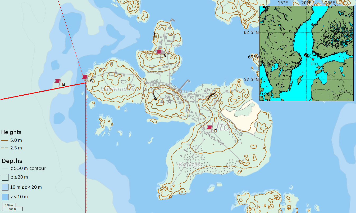
Figure 1Location of the island of Utö in the Archipelago Sea. The research installations on the island consist of the Utö Atmospheric and Marine Research Station and its flux tower (A), the inlet of the seawater sampling system (B), the Atmospheric ICOS station (C), and a weather and air quality station (D). The red solid lines indicate the wind sector used for sea–air flux measurements (180–260∘) used in this paper, and the dashed line indicates the fetch-limited sea sector excluded from the current analysis.
The Marine Research Station and its flux tower are located on the western side of the island. To the west of the shore, the water depth quickly deepens to 80 m. The closest shoal, Tratten, is located 1.4 km to the southwest and has an area of 0.007 km2.
The mean annual wind speed at Utö is 7.1 m s−1 (Pirinen et al., 2012). On average, the minimum monthly wind speed occurs in July (5.6 m s−1) and the maximum in December (8.9 m s−1). The wind blows approximately 60 % of the time from the sector between south and northwest (Fig. 1), providing a good temporal coverage for the sea–air flux measurements.
The mean annual air temperature in Utö is 6.6 ∘C, whereas the mean annual surface seawater temperature at the depth of 5 m is 8.1 ∘C (Laakso et al., 2018). In deep water (at 50 m depth), the mean annual seawater temperature is 4.4 ∘C. The maximum monthly mean air temperature (16.7 ∘C) is observed in July, whereas the seawater at 5 m depth reaches its maximum temperature (16.1 ∘C) in August. The minimum temperature of air (−2.1 ∘C) occurs in February, while the temperature of the surface seawater is at its minimum (1.0 ∘C) in March. On average, there is ice around Utö every few years, with a typical ice cover duration ranging from 1 to 3 months.
Unlike the oceans, the carbon cycle in the Baltic Sea is heavily influenced by biological activity. The partial pressure of CO2 (pCO2) in surface water has its maximum 60 Pa (600 µatm) during winter, when biological activity is diminished, mineralization prevails and mixing processes transport CO2-rich seawater to the surface (Wesslander, 2011). During summer, pCO2 in surface water declines to approximately 10 Pa (100 µatm) as a result of primary production. Due to the annual cycle of primary production, the Baltic Sea is a source of CO2 to the atmosphere in winter and a sink in summer. Upwelling and the diurnal biological cycle generate short-term variations in the surface water pCO2.
2.2 Instrumentation
A 9 m tall micrometeorological tower was placed on the western shore of the island (Figs. 1 and 2). The tower is mounted on a cliff that has no vegetation. The base of the tower is approximately 3 m above the mean sea level, and the horizontal distance between the tower and the sea is approximately 4 m. In this paper, we utilize data from the open sea sector towards the Baltic Proper (180–260∘). The fetch in the sector 260–340∘ may be limited, and, as the anemometer base potentially disturbs the flow, the data from this sector were not included in this study.
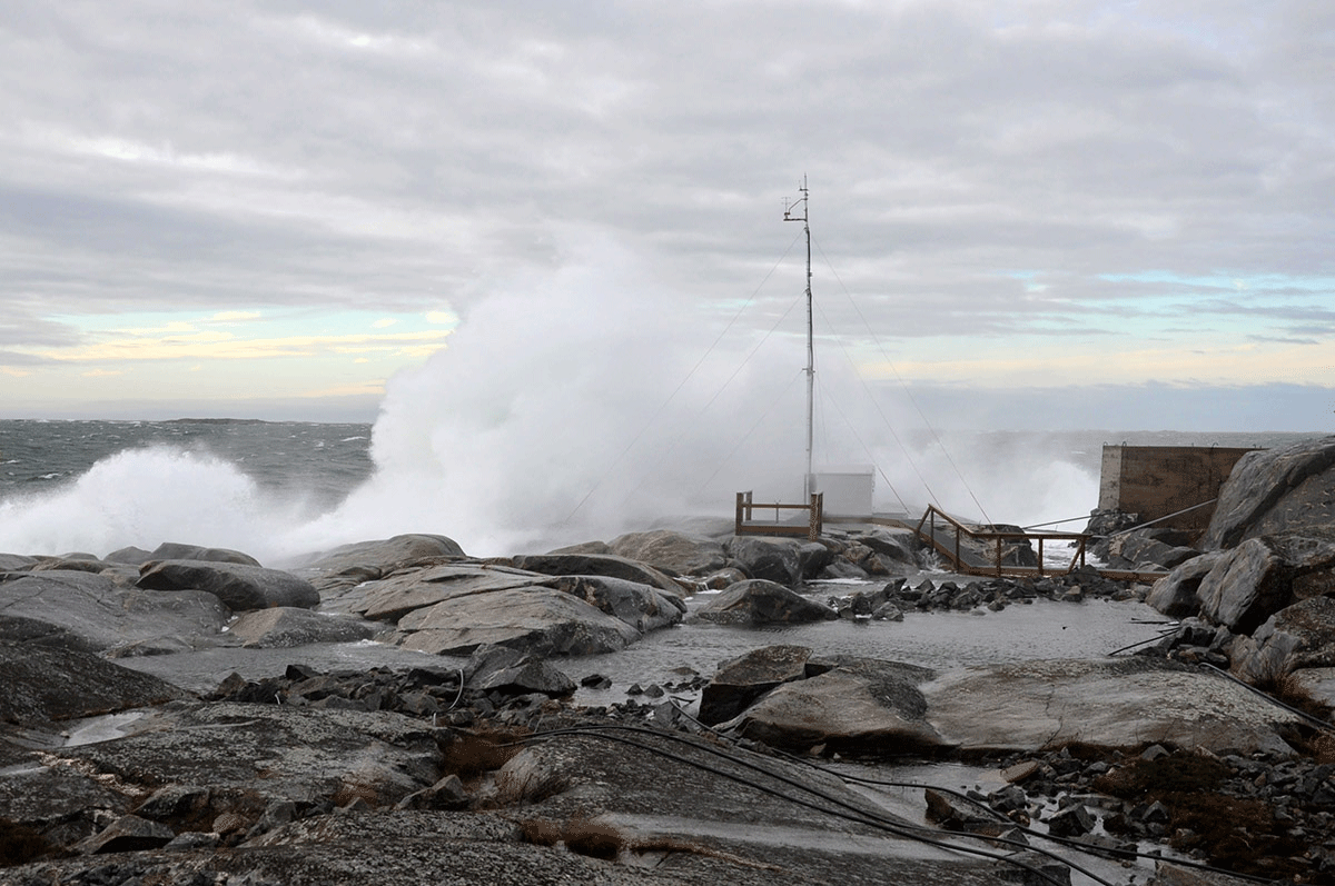
Figure 2The flux tower (height 9 m) on the shore of the island of Utö during a wintertime westerly storm (photo by Ismo Willström).
Air velocity components together with air temperature, T, were measured with an acoustic anemometer/thermometer (uSonic-3, Metek) attached to the top of the tower (11.5 m a.s.l.). CO2 and H2O molar fractions were measured by using two closed-path differential non-dispersive infrared gas analyzers (LI-7000, LI-COR) that were placed in a 1.5 m tall instrument hut close to the tower (Fig. 2). The inlets of both sample flows are protected with a grate and are located directly beneath the anemometer; the distance between the inlets and the lower anemometer transducers is 30 cm. The outside parts of the tubes are approximately 10 m long and are made of Teflon (inner diameter of 3.175 mm) and steel (inner diameter of 4.0 mm). The steel-tube sample line is equipped with a virtual impactor (see Appendix A), to protect the instrument from possible exposure to liquid water, and a 30 cm long PD-100T-12-MKA drier (Perma Pure) to attenuate water vapor fluctuations. The drier is based on the partial pressure difference that drives water vapor from the sample air to the purge stream through a Nafion membrane. The sample air leaving the gas analyzer of the test setup is directed to the purge cell of the drier. Thus, the total pressure difference drives the attenuation of water vapor fluctuations. Nafion driers are found to have only a small permeability to CO2 (Welp et al., 2013).
Inside the instrument hut, the flow continues in 1 m long Bev-A-Line tubes, which are protected by Teflon filters and connected to the analyzers. Data are logged at a 10 Hz frequency and transmitted through the Internet to a server. The hut temperature is regulated using a fan and a radiator, since large temperature changes influence the performance of the CO2 analyzers.
An external pump is used for producing a sample flow at a rate of approximately 6 L min−1 for both setups. We operate the LI-7000 gas analyzers in the absolute mode, which means that a small stream of zero gas (0 ppm CO2) is constantly flowing through the reference cell of both analyzers. The same zero gas flows through both analyzers. The actual zero gas bottle (40 L) is located at the station, and a small stream of zero gas flows continuously to the gas analyzers in the instrument hut. The gas analyzers are calibrated with zero and span (364.4 ppm CO2) gases every 3 months. After each calibration, the Teflon filters are renewed and the virtual impactor is cleaned. The outside tubes are washed with an isopropyl alcohol–water mixture annually. At the same time, the Bev-A-Line tubes and the internal chemicals of the gas analyzers are renewed, and the optical paths are cleaned.
The setup with the Nafion drier and the virtual impactor is referred here to as the “test setup”, and the other setup as the “standard setup”. The standard setup represents a typical closed-path gas analyzer-based eddy covariance setup commonly applied in terrestrial ecosystems (Aurela et al., 2015). The test setup is an improved version of this configuration, designed especially for a marine environment where water vapor and sea spray are likely to give rise to problems.
2.3 Data processing
2.3.1 Flux calculation
As the LI-7000 gas analyzer does not directly provide molar fractions with respect to dry air, we first calculated the dilution-corrected CO2 molar fraction as
where cw is the uncorrected molar fraction of CO2 and q is the molar fraction of H2O.
It is assumed that the long pipe lines, both Teflon and steel, strongly attenuate the temperature fluctuations, and thus there is no need for correcting for expansion/contraction effects in the sample air (Rannik et al., 1997). The eddy covariance mass flux was calculated from the fluctuations of molar fractions of an atmospheric quantity, χ, and vertical wind speed, w:
where ρd is the dry-air density. The primes denote the 10 Hz fluctuations with respect to a time average, and the overbar denotes arithmetic averaging. An averaging period of 30 min was adopted. For each period, the time delay between the acoustic anemometer and gas analyzer data flows was determined by maximizing the (absolute) covariance in Eq. (2) within a predefined time window, and a double coordinate rotation was applied to ensure zero vertical wind speed.
The fulfillment of several theoretical requirements for the eddy covariance measurements was considered. The nonstationarity of the flux measurements was analyzed by comparing the average of the CO2 fluxes calculated for 5 min subperiods (, where i is the index of the subperiod) with the 30 min flux () similarly to Foken and Wichura (1996). The relative nonstationarity, RN, for a given variable, ζ, was defined as
In the case of CO2 flux, . Here, a 30 min period is regarded as stationary if both of the CO2 flux measurements fulfill the condition . To test the development of turbulence, integral turbulent characteristics of temperature and vertical velocity were compared to universal surface-layer functions (Thomas and Foken, 2002). It is assumed that turbulent transport of all scalars (T, CO2 and H2O) are similar, and thus only the characteristics of T are examined here. For this examination, only stationary conditions within the sea sector are included. An observation is also discarded if a positive momentum flux is measured, as these can be considered a sign of flow nonstationarity (Yang et al., 2016).
2.3.2 Spectral analysis
Spectral analysis was carried out in order to evaluate the high-frequency attenuation of the fluxes. High-frequency attenuation was examined by calculating the cospectra between w and c () and q () and comparing these with the corresponding cospectra between w and T (CowT). For this purpose, it is assumed that the high-frequency end of CowT is unattenuated and that the atmospheric turbulent transport of heat, water vapor and CO2 is similar.
Before calculating the half-hourly cospectra using the discrete Fourier transform, the 10 Hz data were linearly detrended and the Hamming window was applied. The cospectra were normalized with the corresponding covariances and interpolated into 64 logarithmically equally spaced bins.
Observations with an appropriate wind direction (180–260∘) and stationary conditions () were accepted for spectral analysis. A total of 607 half-hour periods met these criteria. Next, we discarded small fluxes (< 0.1 ), after which we had 381 half-hour periods. Furthermore, a cospectrum was discarded if its peak was not within a predefined range (0.01–0.5 Hz). A total of 283 cospectra passed this frequency range criterion. Also, a cospectrum was discarded if its normalized peak size () was not within predefined range (0.1–1.0). Thus, 238 observations from a 4-month period were used for the spectral analysis.
The spectral attenuation of the flux as a function of frequency, f, was described by an exponential transfer function, Γ:
where f0 is the half-power frequency at which the ratio of cospectral densities is 0.5. Using a nonlinear least squares fit, the transfer function in Eq. (4) was fitted to the ratio of or to CowT. To fit the transfer function, the cospectra were normalized so that their peaks were leveled. Also, four outermost points from the high-frequency end were discarded because these points may easily be biased due to the division by very small number and 20 outermost points from the low-frequency end were discarded because these points do not play role in the high-frequency attenuation. In the case of H2O fluxes, a power-law relationship between f0 and RH was additionally derived similarly to Mammarella et al. (2009).
To correct for the high-frequency attenuation of fluxes, the universal CowT equations reformulated by Horst (1997) from those originally presented by Kaimal et al. (1972) and Kaimal and Finnigan (1994) were used as a reference. As the shape of this universal cospectrum depends on stability and wind speed, the attenuation for each 30 min flux was calculated as a function of these meteorological parameters.
2.4 Auxiliary data
In addition to the flux measurements, we present here data of the dissolved CO2 concentration in surface seawater, which is measured using a SuperCO2 system (Sunburst Sensors LLC) connected to a submersible pump. The SuperCO2 instrument consists of a showerhead equilibration chamber and an infrared gas analyzer (840A, LI-COR). The measured CO2 molar fraction is corrected for H2O dilution effect using the measured H2O molar fraction. Since this CO2 measurement is not carried out using pre-dried sample air, a H2O cross-sensitivity effect on CO2 is possible but likely small compared to the other error sources, such as spatial heterogeneity in seawater CO2 concentration. To account for sensor drift, the flows of four reference gases are directed into the instrument every 4 h, and a linear correction is calculated from these calibration measurements. The system automatically cleans the equilibration chamber with hydrogen peroxide periodically. The bottom-moored, floating inlet for seawater is located 250 m west of the station (Fig. 1) and is kept approximately 4.5 m below the mean sea level: the sampling depth typically varies within 4.0–5.0 m. The water depth at this location is 23 m. Since sample water exchanges heat with the pipe and its surroundings, a correction for this temperature effect was applied according to Takahashi et al. (1993):
where is the temperature-corrected partial pressure of CO2, is the observed partial pressure of CO2, Tin is seawater temperature measured close to the inlet and Teq is the temperature measured in the tubing right before the equilibration chamber. Additionally, sea bottom temperature at 23 m depth below the inlet is measured by an internal thermometer inside an acoustic Doppler current profiler (ADCP).
The atmospheric concentration of CO2 at the height of 57 m was measured at the atmospheric station run by Integrated Carbon Observation System, ICOS (C in Fig. 1). At this station, the dry molar fraction of CO2 is measured using a very stable cavity ring-down spectroscopy technique (G2401, Picarro). For more information on the atmospheric ICOS measurements at Utö, the reader is referred to Kilkki et al. (2015).
3.1 Suitability of the site for eddy covariance measurements
3.1.1 Environmental conditions
The measurement period (1 July–1 November 2017) represents the late summer and autumn seasons of the carbon cycle, when biological activity diminishes and the sea–air pCO2 difference shifts from negative to positive (Fig. 3e). At the beginning of this period, from July to mid-August, the atmospheric pCO2 exceeded that in the sea, and the sea acted as a sink of atmospheric CO2. The average sea–air pCO2 difference from July to mid-August was 8.0 Pa. During the latter part of August, the sea turned into a source as a result of diminished primary production. The efflux was enhanced when thermal stratification broke down and CO2-rich water surfaced at the beginning of September, resulting in increased surface pCO2. After this event, the partial pressure difference stayed predominantly within 10–20 Pa for the rest of the measurement period, showing only occasional deviations from this range.
The values reported for the sea surface pCO2 represent conditions at the depth of 4.5 m at a single point 250 m away from the flux tower, within the flux measurement sector. In some cases, this location may not represent the carbonate conditions of the whole sea sector area. Especially during the beginning of the measurement period, it is possible that there are horizontal differences in the surface pCO2 due to variations in biological activity (Rutgersson et al., 2008). During other periods, the horizontal differences are likely to be small in the open sea areas, and the surface sea layer is likely to be well mixed at least to the depth of 4.5 m. Thus, we assume that our pCO2 observations represent the surface conditions.
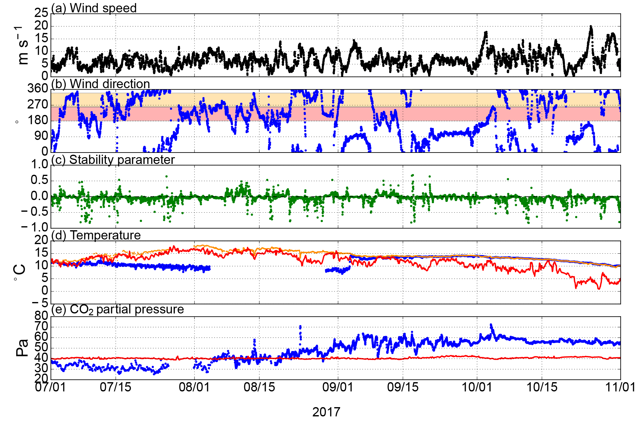
Figure 3Environmental conditions at Utö in July–November 2017: (a) wind speed, (b) wind direction (red band indicates the directions used for sea–air flux measurements in this study, and yellow band indicates additional directions that will be considered in the future), (c) stability (z∕L), (d) air temperature (red) and sea temperature at 4.5 m depth (orange) and at 23 m depth (blue), and (e) CO2 partial pressure in air (red) and CO2 partial pressure in seawater at 4.5 m depth (blue). Wind speed, wind direction, stability and air temperature were measured in the flux station (A in Fig. 1). Seawater temperatures and pCO2 were measured at the inlet (B in Fig. 1). The pCO2 in air was measured at the ICOS station (C in Fig. 1).
During our study period, the wind blew from the sea sector (180–260∘) for 28 % of the time (Fig. 3). This caused gaps in the sea–air flux time series; for instance during the last 2 weeks of September, the wind directions were unsuitable for sea–air exchange measurements. The average wind speed within the marine wind sector was 6.9 m s−1. Stability was mostly near neutral. The vertical rotation angle within the sea sector during the measurement period varied within 0–5∘ with a mean of 3.1∘ and a standard deviation of 1.4∘, indicating that the flow divergence due to the cliff is limited. A small part (3.7 %) of the momentum fluxes measured in the marine sector were positive, and thus the corresponding CO2 flux data were discarded.
In July, air temperature was still gradually increasing, and it reached 18 ∘C by the end of the month. From the beginning of August, both air and sea surface temperature decreased approximately linearly. During the last 3 months, surface seawater cooled by 7 ∘C and air by 10 ∘C.

Figure 4Normalized cospectral densities of (a) the test setup and (b) the standard setup, and (c) CowT (green) and Cowq (yellow). The solid lines represent the median cospectra, and the dashed lines represent the 10th and 90th percentiles. The black line is the model CowT (Horst, 1997). (d) Ratios of cospectral densities (dots) and the fitted exponential transfer functions (solid lines), where red indicates the standard setup, and blue indicates the test setup.
3.1.2 Spectral characteristics
The cospectra of both measurement setups agreed well with the modeled cospectrum (Horst, 1997) in all frequencies (Fig. 4). The low-frequency ends of the measured cospectra approach zero in a similar way to the modeled cospectrum.
The attenuation of the highest frequencies was slightly higher in the more complex tubing: of the test setup (with a drier and a virtual impactor) diverged from the modeled CowT at a slightly lower frequency than that of the standard setup. The half-power frequency for the standard and test system was 0.78 and 0.61 Hz, respectively. These values were used to correct the CO2 fluxes according to the model cospectrum. The average high-frequency correction of the CO2 flux during the measurement period was 16 % for the test setup and 12 % for the standard setup.
The drier and virtual impactor added approximately 1 m to the length of tubing, which only has a minor effect on the attenuation of turbulent fluctuations. However, the virtual impactor forms a 90 ∘ angle to the tubing, which can stabilize the flow, making it laminar at a higher Reynolds number, Re, than in a straight tube (Lenschow and Raupach, 1991). It would be ideal to have turbulent conditions in the tubes, because scalar fluctuations dampen less in a turbulent pipe flow due to the more uniform velocity profile (Lenschow and Raupach, 1991). At low temperatures (0 ∘C), Re of the standard setup was calculated to be 2980, whereas in the test setup it was 2380. By using the tube attenuation equations of turbulent flow presented by Massman and Ibrom (2008), the half-power frequencies were 13.7 and 7.2 Hz for the standard and test setup, respectively. Thus, at low temperatures, fluctuation attenuation due to transport in the tubes is not likely to affect the measurements. However, at higher temperatures (20 ∘C), the Reynolds number of the test setup (2100) falls into the laminar flow region, because kinematic viscosity increases with increasing temperature. By using the tube attenuation equations for laminar flow by Lenschow and Raupach (1991), the half-power frequency of the test setup at 20 ∘C was only 1.4 Hz, which is still higher than the empirically determined f0.
The high-frequency attenuation of H2O signals of the standard setup was corrected in order to accurately compare the CO2 flux measurements with different setups as a function of latent heat flux. The high-frequency attenuation of H2O flux of the standard setup was marked: f0 ranged between 0.04 and 0.22 Hz, decreasing with increasing RH, which varied within 48–100 %. This attenuation is caused by sorption and desorption of water vapor at the walls of the tubings (Massman and Ibrom, 2008). During typical humidity conditions (RH=80 %), the flux attenuation is 44 % of the real H2O flux. The of the test setup was found to be distorted in all frequencies.
3.1.3 Stationarity
In order to evaluate the quality of our measurements, several theoretical assumptions of the eddy covariance method were analyzed. The flux footprint area was found to be horizontally homogeneous (Appendix B), and turbulence was well developed as integral turbulence characteristics could be expressed as functions of stability parameter (Appendix C). In this section, we analyze the fulfillment of the stationarity assumption and determine the effect of CO2 flux nonstationarity on the CO2 fluxes.
Over half of the flow conditions for which the CO2 flux was determined, 65 %, were found to be nonstationary; i.e., the difference between the 30 min flux and the mean of the corresponding 5 min fluxes exceeded 30 %. Overall, 91 % of data were discarded due to unsuitable wind direction, nonstationarity or a positive momentum flux.
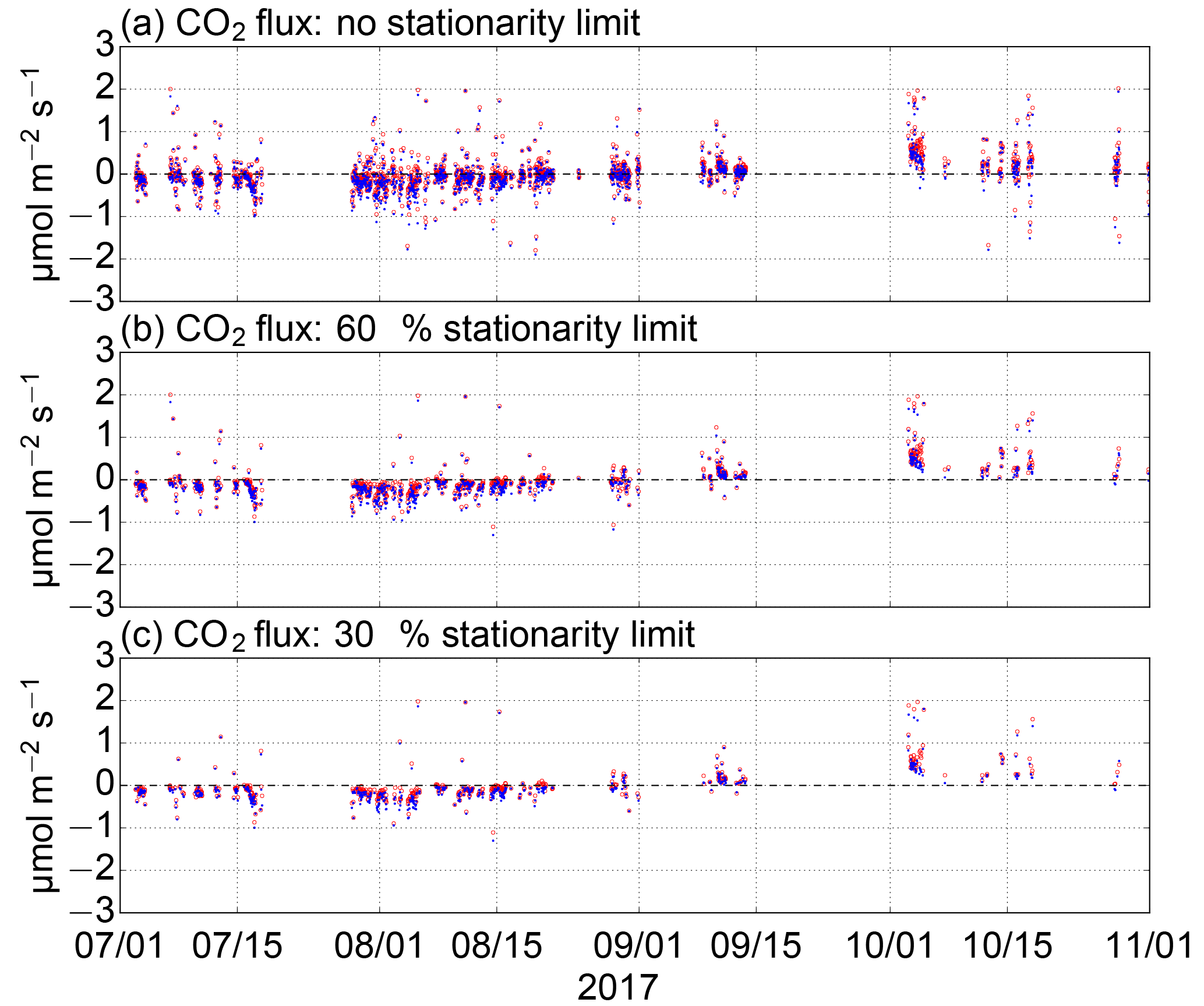
Figure 5The effect of removal of nonstationarity cases on the CO2 flux data: (a) no stationarity limit, (b) and (c) . Red circle refers to the standard setup, and blue dot to the test setup.
We found that this stationarity criterion removed unphysical values effectively (Fig. 5). During July, the partial pressure difference was negative (−9.3 Pa on average), and thus downward (negative) fluxes were expected. Relaxing the stationary limit from 30 % to 60 % had only a small effect on data filtering. When no stationarity limit was applied, 20 % and 25 % of CO2 sea–air fluxes that were measured during July 2017 by the test and standard setup, respectively, and were expected to be negative were positive. When the 60 % stationarity limit was used, only 5 % (test) and 6 % (standard) of the measured CO2 fluxes were positive. With the 30 % stationarity limit, these numbers were only slightly lower: 3 % and 4 %, respectively.
Similarly high rejection rates have been obtained in previous studies. Miller et al. (2010) reported that 65 % of the sea–air CO2 flux measurements failed a stationarity test in which the 13.7 min fluxes were compared with the averages of 3.4 min fluxes, and they assumed that CO2 concentration heterogeneity could be a reason for the high rejection rate. Likewise, Blomquist et al. (2014) concluded that horizontal CO2 concentration gradients caused by continental pollution sources can reduce the number of stationary situations. At Utö, concentration gradients may be produced by the horizontal heterogeneity due to the land–sea interface and the variations in marine primary production.
We examined how the absolute change in CO2 concentration during the averaging period of 30 min relates to nonstationarity of CO2 fluxes (Fig. 6). The change in CO2 concentration was calculated as a difference in the mean CO2 molar fraction of the last 30 s and the first 30 s. Typically, a change larger than 1 ppm was associated with rejection of the measurement due to the nonstationarity of CO2 flux. Only 14 % and 18 % of the sea–air CO2 fluxes for the test and standard setup, respectively, passed the stationarity test with the 30 % limit, for the cases with a CO2 concentration change larger than 1 ppm. For the cases where CO2 concentration changed more than 2 ppm during the averaging period, only 4 % and 6 % of sea–air CO2 fluxes passed this stationarity test.
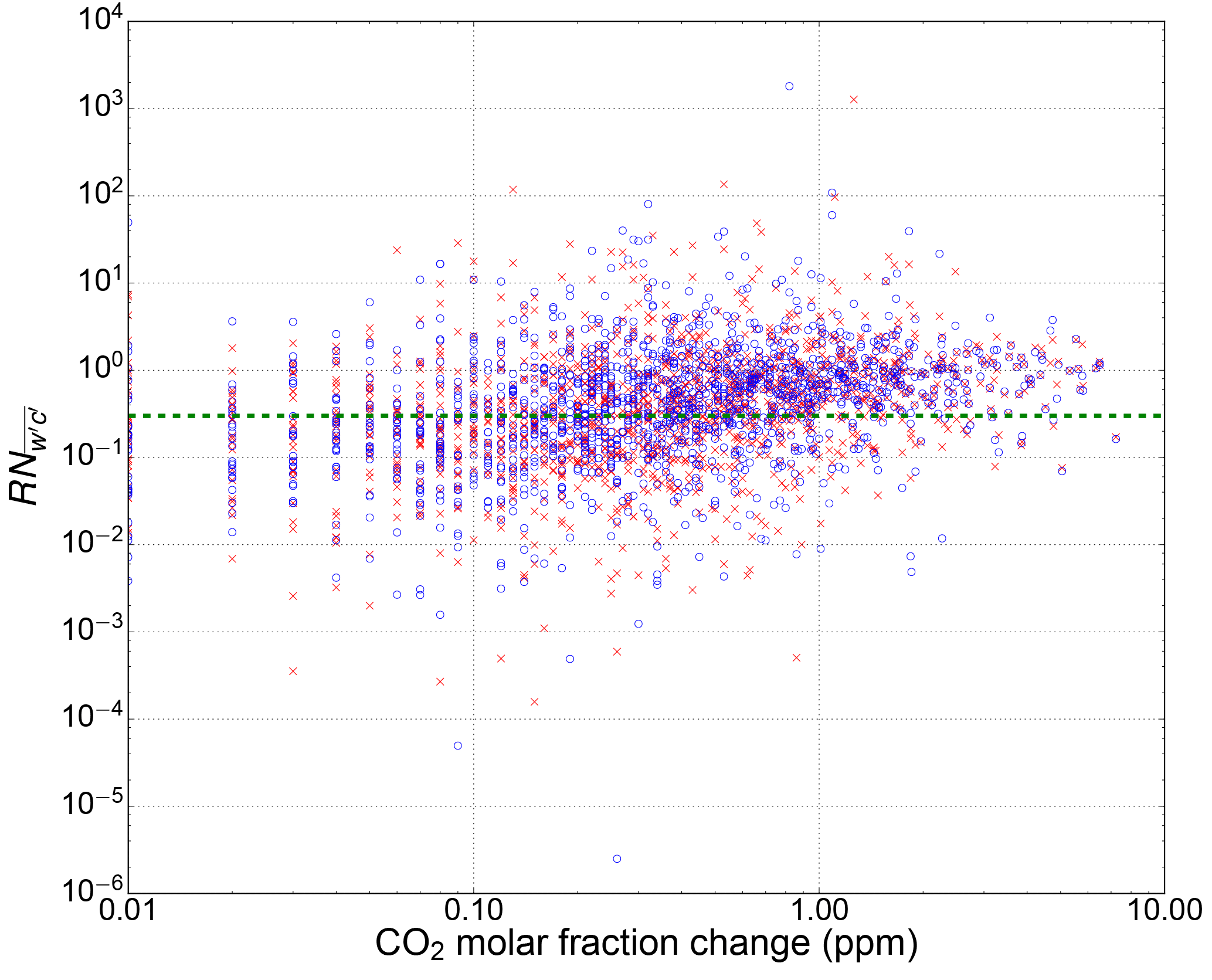
Figure 6Relative nonstationarity of CO2 flux as a function of the absolute change in CO2 concentration during the averaging period: standard (red cross) and test (blue circle) setups. The green dashed line indicates the limit of .
If the timescale of the processes generating nonstationarity were less than the averaging time, it would be possible to reduce the amount of discarded nonstationary data by shortening the averaging time. To test for nonstationarity with shorter averaging periods, we calculated CO2 fluxes for 15 min periods, which were compared with the average of 2.5 min CO2 fluxes. It was found that this increased the number of accepted data only a little: by 6.1 % for the standard setup and 1.9 % for the test setup.
3.2 Setup comparison
The observed direction of the sea–air CO2 fluxes was mainly consistent with the pCO2 difference between the sea and the atmosphere, and both setups showed similar fluxes most of the time (Fig. 7). The standard setup tended to show slightly more positive fluxes than the test setup. In July, the pCO2 difference was negative, and the mean sea–air CO2 flux measured with the standard and test setup was −0.163 and −0.226 , respectively. During the latter part of August (15–31 August), when the pCO2 difference was shifting from negative to positive, the mean flux measured with the standard system (−0.050 ) was close to zero, while the test system still showed clearly negative fluxes (mean −0.122 ). During August, the highest latent heat fluxes of the measurement period were measured, peaking at 120 W m−2. During September, low latent heat fluxes (3.3 W m−2 on average) were observed and both measurements showed closely similar monthly sea–air CO2 flux: 0.188 (test) and 0.158 (standard). The highest absolute monthly CO2 fluxes were measured in October, when pCO2 difference was continuously high (16.6 Pa on average) and wind speed peaked occasionally, resulting in monthly sea–air CO2 flux averages of 0.524 and 0.434 by the standard and test setup, respectively.

Figure 7Sea–air fluxes of (a) CO2 and (b) water vapor: standard setup (red circles) and test setup (blue crosses). Only the fluxes originating from the southwestern open sea sector (Fig. 1) are shown.
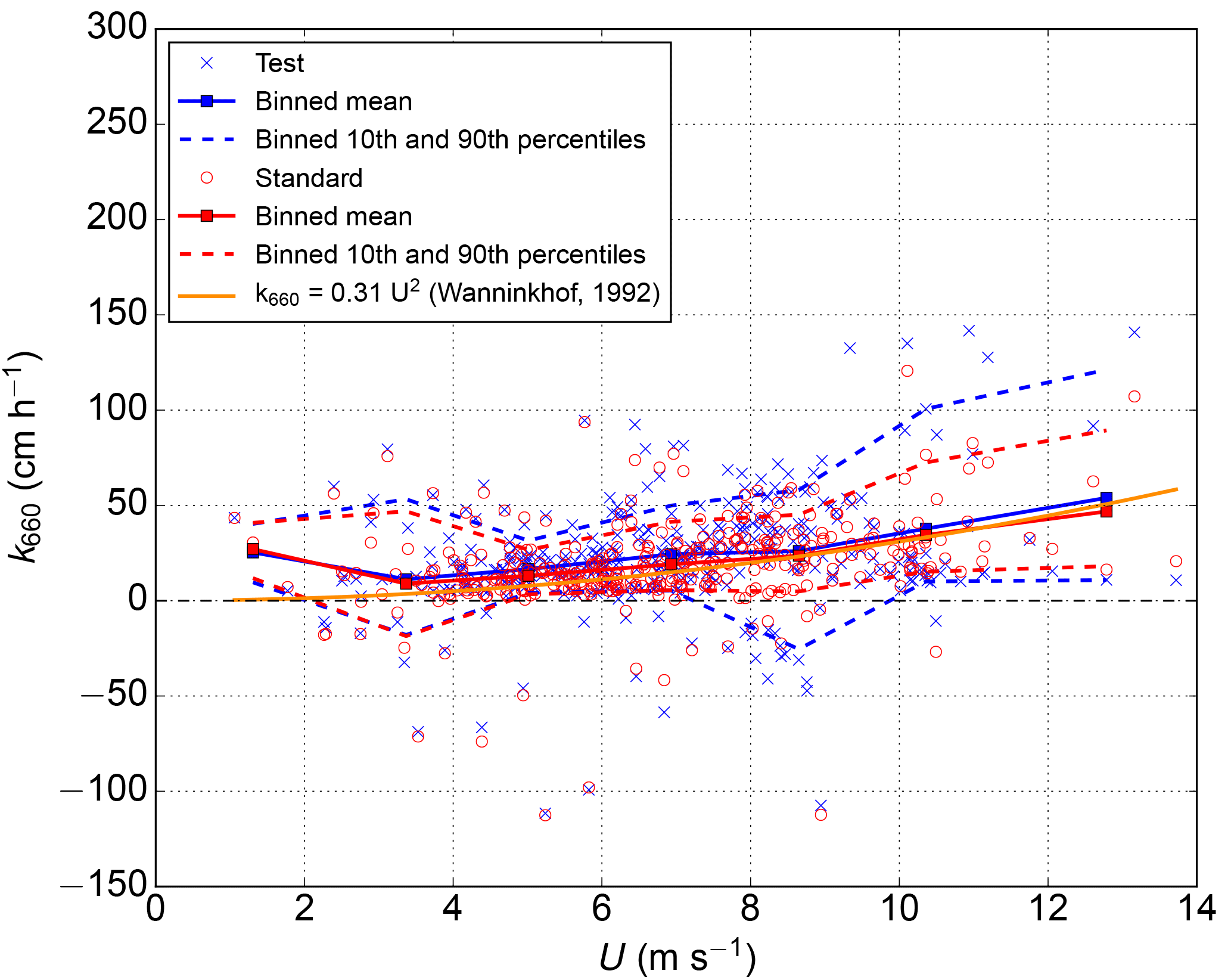
Figure 8Measured gas transfer velocities as a function of wind speed. The orange line is the parametrization by Wanninkhof (1992).
As no previous measurement data are available for comparison, we validated the magnitude of the measured air–sea CO2 fluxes roughly by calculating the gas transfer velocity () from our data and compared it with the universal parametrization proposed by Wanninkhof (1992). Schmidt number (Sc) and solubility (K0) of CO2 were calculated according to Wanninkhof (1992) and Weiss (1974), respectively. For this comparison, we only included cases in which the absolute partial pressure difference (ΔpCO2) between the sea and atmosphere was larger than 3 Pa. The gas transfer velocities derived from our measurements were mostly in good accordance with predictions (Fig. 8), which lends credence to our flux measurements. During medium wind speeds (3–10 m s−1), the measured k660 values line up closely with the parametrization. More measurements during low (<3 m s−1) and high (>10 m s−1) wind speeds are required to evaluate the relationship between winds peed and k660 during these wind speeds.
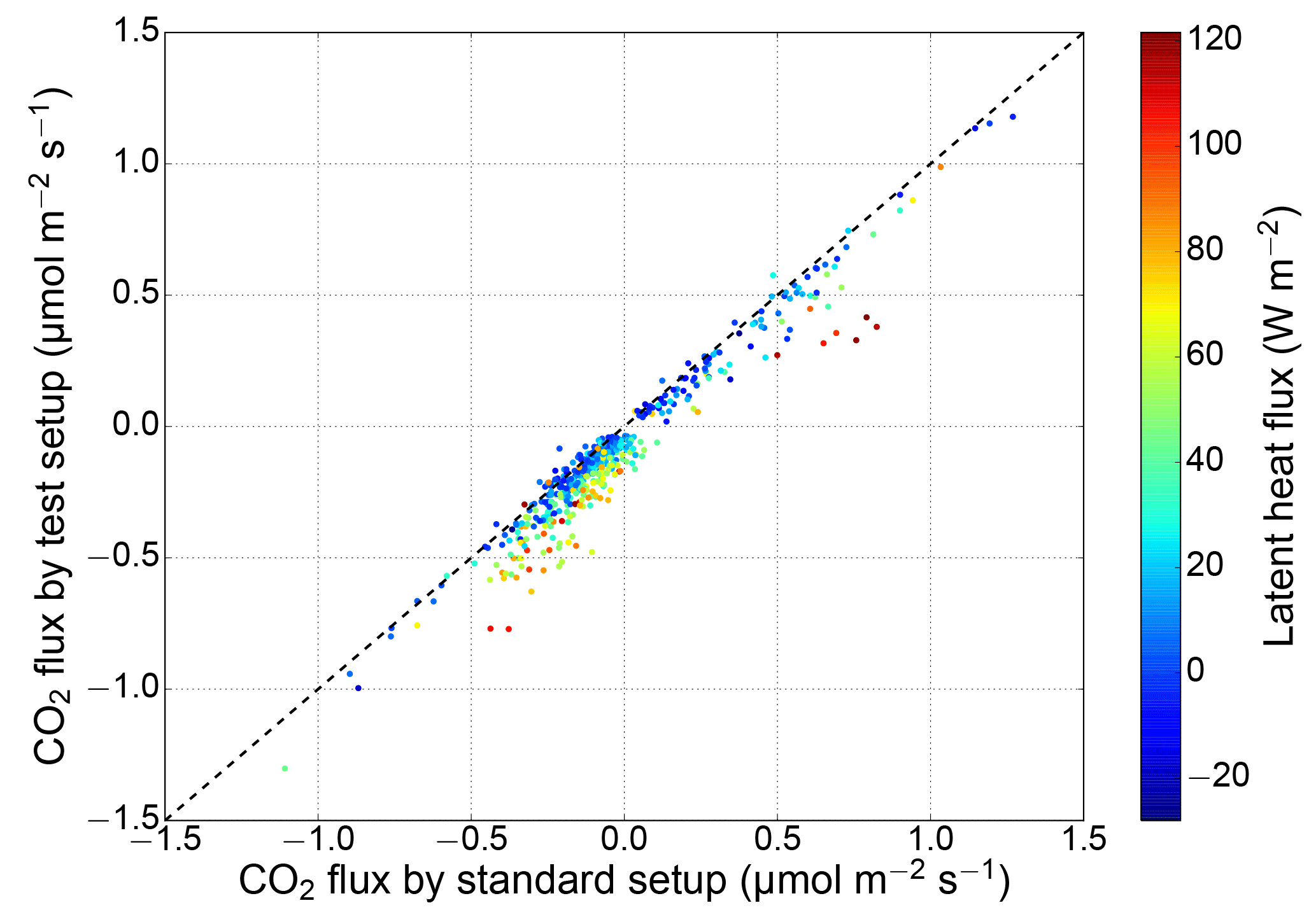
Figure 9The sea–air CO2 flux measured with the standard setup vs. the test setup (equipped with a drier and a virtual impactor). The marker color indicates the concurrent latent heat flux, and the dashed line represents the 1:1 relationship.

Figure 10CO2 flux difference (standard setup–test setup) as a function of latent heat flux for (a) positive and (b) negative water vapor fluxes. The lines show a fitted mean together with the 10th and 90th percentiles for eight logarithmically equally spaced bins.
The Nafion drier eliminated the water vapor fluctuations effectively. The latent heat flux (measured with the standard system) was mostly positive, ranging within −28 to 122 W m−2, with an average of 27 W m−2. The H2O variance measured with the standard setup was 0.021 mmol2 mol−2 on average, whereas the test setup measured the mean H2O variance of 0.001 mmol2 mol−2. Even though the Nafion drier in our setup did not remove water vapor completely, it attenuated the fluctuations at all frequencies, in the same way that the tubing of a closed-path system attenuates temperature fluctuations. Water vapor molar fraction measured by the test setup varied within 2.9–8.8 mmol mol−1, whereas the standard setup showed water vapor values of 5.7–15.7 mmol mol−1. Thus, a total removal of water vapor from the sample air is not required to eliminate the water vapor fluctuations.
A high correlation was found between the two measurement setups (Fig. 9). The Pearson product–moment correlation coefficient between the sea–air CO2 fluxes measured by the setups was 0.97. During low latent heat fluxes (<30 W m−2), the correlation coefficient increased to 0.99. As latent heat flux increases, the standard setup shows more positive CO2 fluxes than the test setup (Fig. 10). These results are in agreement with the conclusions of Landwehr et al. (2014), who found that during low latent heat fluxes the difference between the dried and undried sea–air CO2 flux measurements was very small. This also proves that a Nafion drier (in our case combined with a virtual impactor) does not disturb the CO2 flux measurements.
A comparison of the CO2 flux difference as a function of latent heat flux shows that the error is negligible for very small latent heat fluxes (<10 W m−2). With higher latent heat fluxes (∼60 W m−2), the mean difference is approximately 0.125 . Since the sea–air fluxes of CO2 are typically small, the effect of water vapor on CO2 flux measurement can cause a change in its sign, as observed during the latter part of August. However, as the mean difference increases, the scatter also increases. There are only few data points with negative latent heat fluxes, so no conclusions can be drawn concerning the effect of negative water vapor fluxes on CO2 fluxes.
We showed that the use of the combination of a virtual impactor and a Nafion drier did not disturb the measurement of CO2 fluxes. Closed-path instruments are typically protected by one or two Teflon filters (one close to the inlet and another next to the instrument), which should prevent any liquid water from reaching the instrument. However, the use of a Teflon filter close to the inlet may be unpractical, as a regular change of the filter in high-sea-spray conditions may prove laborious. In such a case, we suggest a virtual impactor as an option for the protection of the instrument and the tubing from water and sea salt.
In this paper, we presented new sea–air CO2 flux measurements, comparing two closed-path gas analyzer setups installed on a shore of an island in the Baltic Sea. One of the setups was equipped with a drier and a virtual impactor. By inspecting several theoretical assumptions of the eddy covariance method, we showed that this land-based flux site is capable of effectively monitoring CO2 fluxes between the atmosphere and the sea. The w–CO2 cospectral densities calculated from our data showed an expected behavior with a moderate high-frequency loss. Turbulence was well developed, and the integral turbulence characteristics followed unique functions of stability and friction velocity.
We found that the two closed-path infrared gas analyzer setups showed similar CO2 fluxes when latent heat fluxes were small. The correlation coefficient increased from 0.97 to 0.99 when only the CO2 fluxes during small latent heat fluxes (<10 W m−2) were included. A higher latent heat flux resulted in a positive bias to the undried measurement. During high latent heat fluxes (∼60 W m−2), the difference between the CO2 flux measurements was 0.125 on average, which is comparable to the monthly mean sea–air CO2 flux. In July, the CO2 partial pressure in the atmosphere exceeded that in the surface seawater, resulting in negative sea–air CO2 fluxes, with monthly averages of −0.16 and −0.23 for the standard and test (drier) setup, respectively. In October, when the surface seawater had a higher CO2 partial pressure than the atmosphere, the average sea–air CO2 fluxes were 0.52 and 0.43 for the standard setup and test setup, respectively.
Our analysis indicated that, to obtain high-quality sea–air CO2 flux data, a large proportion (65 %) of the original observations had to be discarded for nonstationarity. If the nonstationary cases were not discarded, 20 %–25 % of the sea–air CO2 fluxes in July had a wrong sign, whereas only 3 %–4 % of the measured fluxes had an unphysical direction if the nonstationary cases were rejected. This nonstationarity was found to be linked to the changes in atmospheric CO2 concentration during the averaging period. A change larger than 2 ppm was associated with a rejection rate of 94 %–95 % due to nonstationarity. The occurrence of nonstationary conditions was random in time, whereas unsuitable wind directions produced long, continuous gaps in the measurement time series. For the calculation of a CO2 budget, these gaps must be filled, for instance by using the measured pCO2 difference and a gas transfer velocity parameterized as a function of wind speed. Thus, continuous measurements of surface seawater and atmospheric CO2 concentration at the Utö station provide useful additional data for the calculation of sea–air CO2 flux exchange.
We showed that the use of the combination of a virtual impactor and a Nafion drier did not disturb the CO2 flux measurement. While this configuration generated a slightly higher flux loss, we opt for this alternative for its reduced water vapor cross-sensitivity and better protection against sea spray.
The data used in this study can be freely accessed via the Zenodo data repository (Honkanen et al., 2018).
The virtual impactor is based on two perpendicular air streams, which provide a means to separate particles by size (Fig. A1). The sample air stream is divided into minor and major flows: smaller particles are diverted to the major flow, and large particles with higher inertia, in this case water droplets, continue to the minor flow. The 50 % cut point of our virtual impactor was calculated to be 1.2–1.3 µm, i.e., a particle of this size has a 50 % probability of removal, while smaller particles are more likely to enter the major flow.
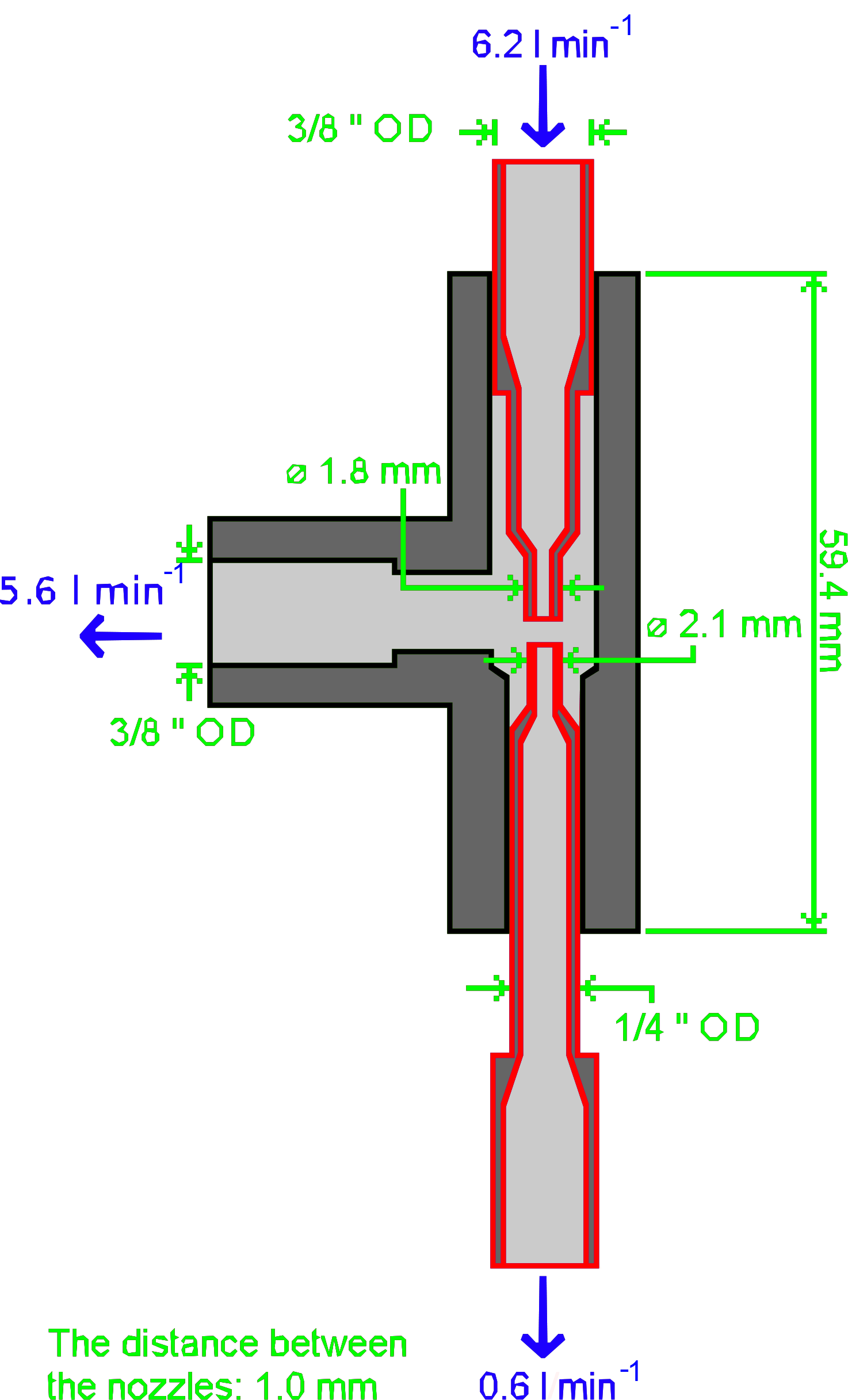
Figure A1Schematics of the virtual impactor attached to the test setup. OD stands for outside diameter. The red pipes are enclosed by the black outer case. A more detailed figure is available on request.
Horizontal homogeneity within the sea sector (180–340∘) was examined in terms of the surface roughness length (z0), which was calculated from the logarithmic wind profile law using data collected during neutral conditions, (Fig. B1).
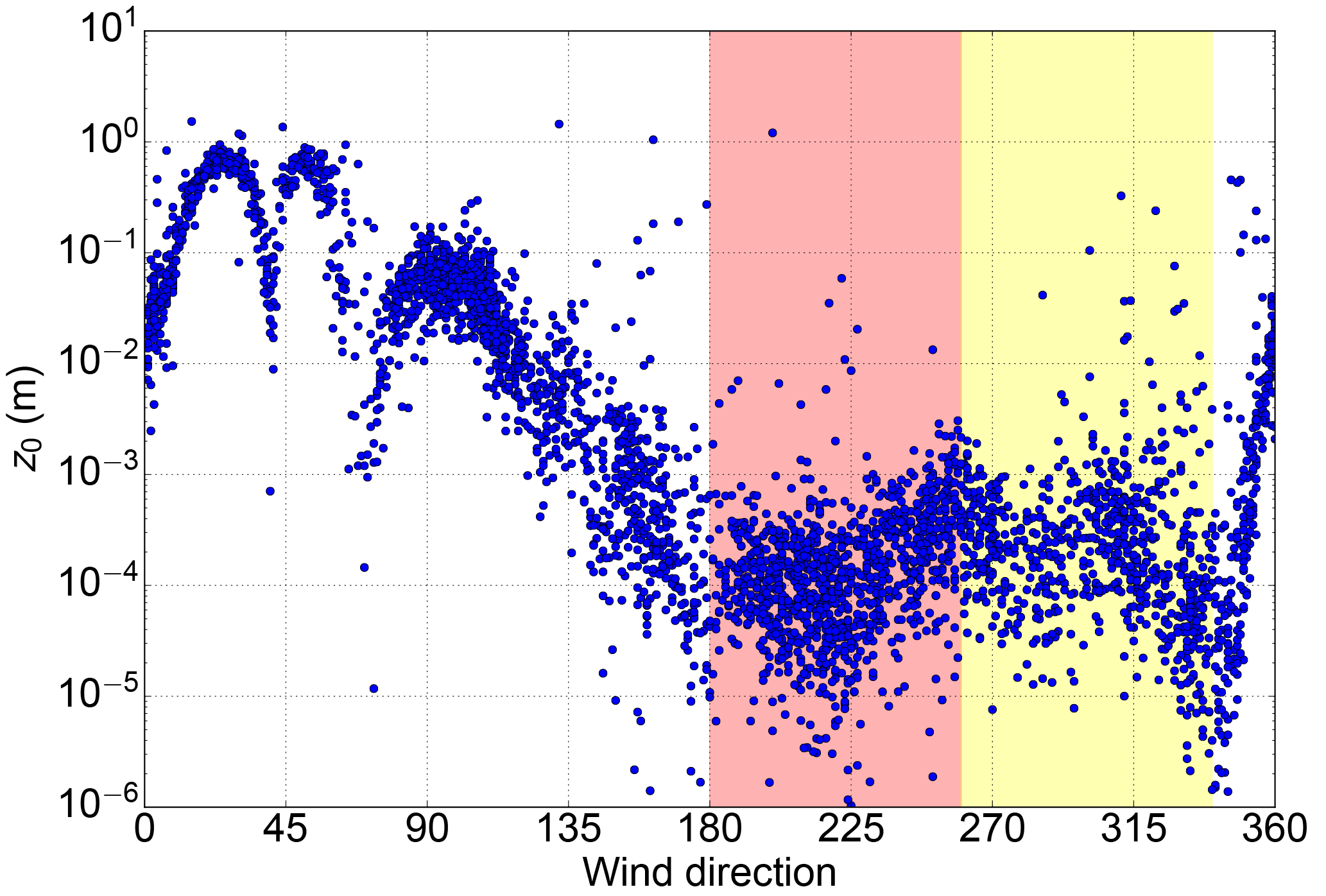
Figure B1Surface roughness length as a function of wind direction. The red band indicates the directions that are considered the open sea sector used in this paper, and the yellow band indicates a wind sector that potentially provides useful data that were excluded from the present study.
The sea sector is clearly visible in the expected range of 180–340∘, where z0 is mainly lower than 1 mm. Outside this sector, z0 is clearly higher, up to 1 m in northeastern wind directions. The sea sector indicated by z0 coincides well with the sector deduced from the geographical map (Fig. 1).
While the sea sector can be considered sufficiently homogeneous, there is scatter in z0 reflecting the fact that it depends on the sea state. Taylor and Yelland (2001) found that over a sea surface z0 depends on the significant wave height and the slope of the wave. Since the measurement site is located on the coast, both the fetch and swell can depend on wind direction.
The Monin–Obukhov similarity theory predicts that statistical turbulence variables within the atmospheric surface layer are unique functions of the stability parameter (z∕L), which combines information about the height above ground, surface shear stress, surface heat flux and buoyant processes. These so-called integral turbulence characteristics have been found to have the same stability dependence over the sea as on land (Smith and Anderson, 1984) and can be used to examine the development of turbulence.
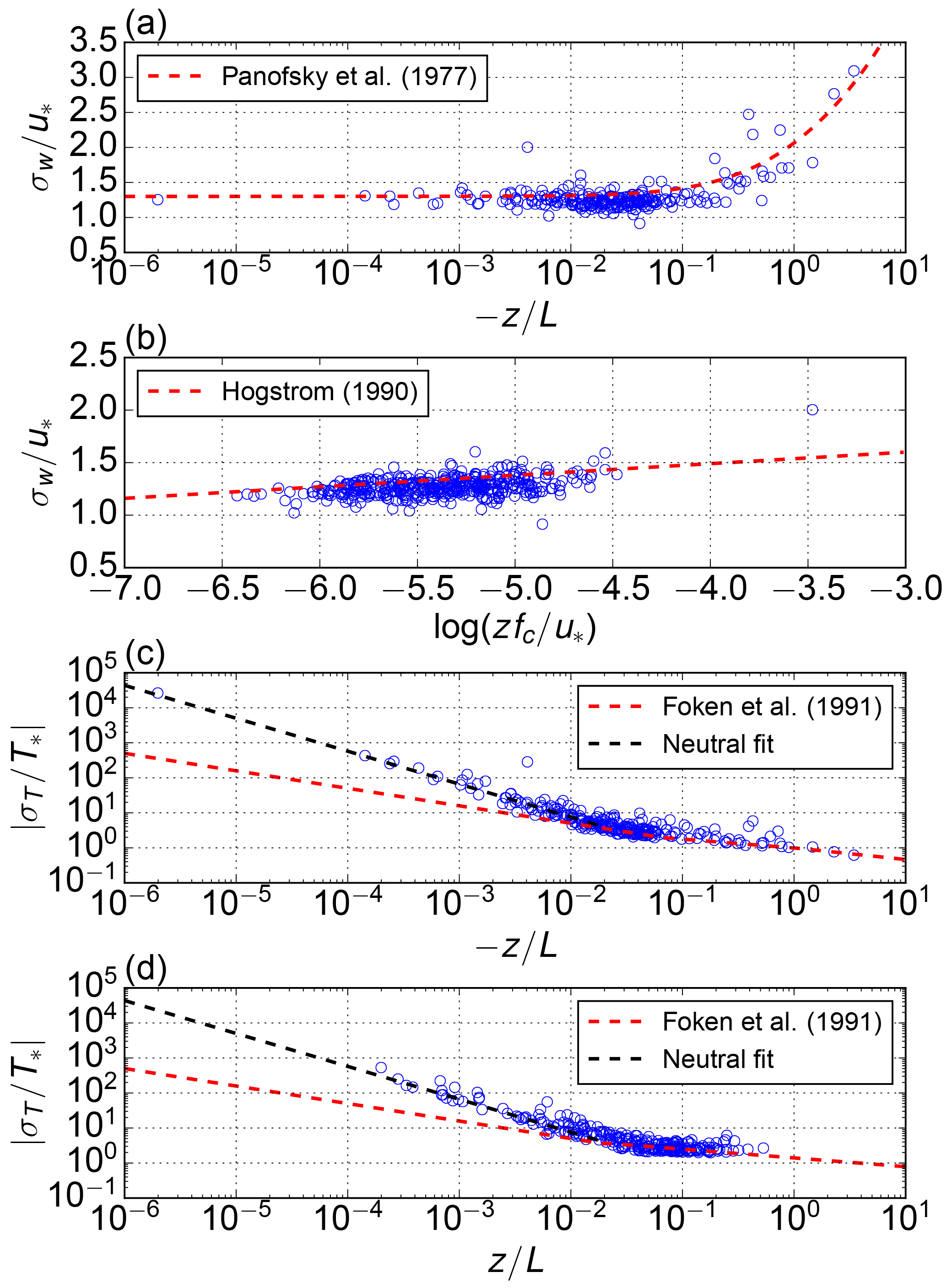
Figure C1Integral turbulence characteristics. (a) as a function of stability parameter z∕L, (b) as a function of , (c) as a function of z∕L during unstable stability and (d) as a function of z∕L during stable stability.
Our data are in accordance with the results of Panofsky et al. (1977), who determined the relationship between the normalized standard deviation of vertical velocity and stability parameter:
where u* is friction velocity, α=1.3 and β=3.0. With large values, the power law of 1∕3 fits our observations well, and the observed approaches a constant of 1.3 in the neutral range similarly to Eq. (C1). Most of the observations fall into the stability range between −0.1 and −0.01. Within this range, the observed is mainly scattered between values 1.0 and 1.5.
However, Monin–Obukhov similarity theory does not consider all the necessary information for describing turbulence characteristics in all conditions; e.g., the effect of Coriolis and pressure-gradient forces are excluded. Högström (1990) showed that during neutral stratification can be described with z; u*; and the Coriolis parameter, fc. Smedman (1990) found that this relationship is valid at widely differing sites, including both terrestrial and marine surfaces. Thus we tested our data with neutral stratification, , against the function proposed by Högström (1990):
where γ=0.11 and δ=1.93. This function provides a reasonable fit to our data and a better description of in the stability range between −0.1 and −0.01 than Eq. (C1) (Fig. C1).
For temperature, we compared the observations to the model of Foken et al. (1991):
Our observations were in accordance with the shape of this relationship, except for the near-neutral stability range, where the observations differ greatly from the model (Fig. C1c–d). As these cases have a very small sensible heat flux, could be biased by division by a small number. However, this is not observed as the slope is well organized, and the spread is small. Our data suggest a steeper relationship should be used in this near-neutral stability range ():
On a logarithmic scale, the slope (−0.94) in our fit is almost twice as steep as the corresponding slope determined by Foken et al. (1991), i.e., −0.5.
Overall, our observations were well organized as a function of stability parameter, or friction velocity in the neutral case, and thus we did not discard any of the data based on the integral turbulence characteristics.
The authors declare that they have no conflict of interest.
MH, JPT, LL and TL were in charge of the conceptualization of the research. Under the supervision of JPT and LL, MH performed data analysis and visualization and prepared the original draft of the manuscript, which was further rigorously reviewed and edited by JPT, LL and TL. TM, SK and LL designed and constructed the flux tower and the pCO2 measurement systems. JH wrote the data management and flux calculation software.
This work was financially supported by the Finnish Meteorological Institute,
the BONUS INTEGRAL project (BONUS Blue Baltic) and the JERICO-NEXT project
(EU – Horizon 2020, 654410). The Integrated Carbon Observation System is
acknowledged for providing the data of atmospheric CO2 concentrations in
Utö. Both reviewers (Gil Bohrer and Brian Butterworth) and the associate
editor (Christof Ammann) are acknowledged for their insightful comments, which
improved the final version of the manuscript.
Edited by: Christof Ammann
Reviewed by: Gil Bohrer and Brian Butterworth
Aurela, M., Lohila, A., Tuovinen, J.-P., Hatakka, J., Penttilä, T., and Laurila, T.: Carbon dioxide and energy flux measurements in four northern-boreal ecosystems at Pallas, Boreal Environ. Res., 20, 455–473, 2015. a
Blomquist, B. W., Huebert, B. J., Fairall, C. W., Bariteau, L., Edson, J. B., Hare, J. E., and McGillis, W. R.: Advances in Air–Sea CO2 Flux Measurement by Eddy Correlation, Bound.-Lay. Meteorol., 152, 245–276, 2014. a, b, c
Chatziefstratiou, E. K., Velissariou, V., and Bohrer, G.: Resolving the Effects of Aperture and Volume Restriction of the Flow by Semi-Porous Barriers Using Large-Eddy Simulations, Bound.-Lay. Meteorol., 152, 329–348, 2014. a
Dabbert, W. F., Lenschow, D. H., Horst, T. W., Zimmerman, P. R., Oncley, S. P., and Delany, A. C.: Atmosphere-surface exchange measurements, Science, 260, 1472–1481, 1993. a
Edson, J. B., Fairall, C. W., Bariteau, L., Zappa, C. J., Cifuentes-Lorenzen, A., McGillis, W. R., Pezoa, S., Hare, J. E., and Helmig, D.: Direct covariance measurement of CO2 gas transfer velocity during the 2008 Southern Ocean gas exchange experiment: wind speed dependency, J. Geophys. Res., 116, C00F10, https://doi.org/10.1029/2011JC007022, 2011. a
Feely, R., Doney, S., and Cooley, S.: Ocean Acidication: Present Conditions and Future Changes in a High-CO2 World, Oceanography, 22, 36–47, 2009. a
Foken, T. and Wichura, B.: Tools for quality assessment of surface-based flux measurements, Agric. Forest Meteorol., 78, 83–105, 1996. a, b
Foken, T., Skeib, G., and Richter, S. H.: Dependence of the integral turbulence characteristics on the stability of stratification and their use for doppler-sodar measurements, Meteorol. Z., 41, 311–315, 1991. a, b
Heinze, C., Meyer, S., Goris, N., Anderson, L., Steinfeldt, R., Chang, N., Le Quéré, C., and Bakker, D. C. E.: The ocean carbon sink – impacts, vulnerabilities and challenges, Earth Syst. Dynam., 6, 327–358, https://doi.org/10.5194/esd-6-327-2015, 2015. a
Högström, U.: Analysis of turbulence structure in the surface layer with a modified similarity formulation for near neutral conditions, J. Atmos. Sci., 47, 1949–1972, 1990. a, b
Honkanen, M., Tuovinen, J.-P., Laurila, T., Mäkelä, T., Hatakka, J., Kielosto, S., and Laakso, L.: Dataset for Measuring turbulent CO2 fluxes with a closed-path gas analyzer in a marine environment (2018) [Data set], Zenodo, https://doi.org/10.5281/zenodo.1425505, 2018.
Horst, T. W.: A simple formula for attenuation of eddy fluxes measured with first-order response scalar sensors, Bound.-Lay. Meteorol., 82, 219–233, 1997. a, b, c
Ibrom, A., Dellwik, E., Larsen, S. E., and Pilegaard, K.: On the use of the Webb-Pearman-Leuning theory for closed-path eddy correlation measurements, Tellus B, 59, 937–946, 2007. a
Jones, E. P. and Smith, S. D.: A first measurement of sea-air CO2 flux by eddy correlation, J. Geophys. Res., 82, 5990–5992, 1977. a
Kaimal, J. C. and Finnigan, J. J.: Atmospheric boundary layer flows – their structure and measurement, Oxford University Press, New York, USA, 1994. a
Kaimal, J. C., Wyngaard, J. C., Izumi, Y., and Cote, O. R.: Spectral characteristics of surface-layer turbulence, Q. J. Roy. Meteor. Soc., 98, 563–589, 1972. a
Kenny, W. T., Bohrer, G., Morin, T. H., Vogel, C. S., Matheny, A. M., and Desai, A. R.: A Numerical Case Study of the Implications of Secondary Circulations to the Interpretation of Eddy-Covariance Measurements Over Small Lakes, Bound.-Lay. Meteorol., 165, 311–332, 2017. a
Kilkki, J., Aalto, T., Hatakka, J., Portin, H., and Laurila, T.: Atmospheric CO2 observations at Finnish urban and rural sites, Boreal Environ. Res., 20, 227–242, 2015. a
Kohsiek, W.: Water vapor cross-sensitivity of open path H2O/CO2 sensors, J. Atmos. Ocean. Technol., 17, 299–311, 2000. a
Kondo, F. and Tsukamoto, O.: Air-sea CO2 flux by eddy covariance technique in the Equatorial Indian Ocean, J. Oceanogr., 63, 449–456, 2007. a
Kondo, F., Ono, K., Mano, M., Miyata, A., and Tsukamoto, O.: Experimental evaluation of water vapour cross-sensitivity for accurate eddy covariance measurement of CO2 flux using open-path CO2/H2O gas analysers, Tellus B, 66, 23803, https://doi.org/10.3402/tellusb.v66.23803, 2014. a
Laakso, L., Mikkonen, S., Drebs, A., Karjalainen, A., Pirinen, P., and Alenius, P.: 100 years of atmospheric and marine observations at the Finnish Utö Island in the Baltic Sea, Ocean Sci., 14, 617–632, https://doi.org/10.5194/os-14-617-2018, 2018. a, b
Lammert, A. and Ament, F.: CO2-flux measurements above the Baltic Sea at two heights: flux gradients in the surface layer?, Earth Syst. Sci. Data, 7, 311–317, https://doi.org/10.5194/essd-7-311-2015, 2015. a
Landwehr, S., Miller, S. D., Smith, M. J., Saltzman, E. S., and Ward, B.: Analysis of the PKT correction for direct CO2 flux measurements over the ocean, Atmos. Chem. Phys., 14, 3361–3372, https://doi.org/10.5194/acp-14-3361-2014, 2014. a, b
Lenschow, D. H. and Raupach, M. R.: The attenuation of fluctuations in scalar concentrations through sampling tubes, J. Geophys. Res., 96, 15259–15268, 1991. a, b, c
Leuning, R. and King, K. M.: Comparison of eddy-covariance measurements of CO2 fluxes by open- and closed-path CO2 analysers, Bound.-Lay. Meteorol., 59, 297–311, 1992. a
LI-COR, Inc.: LI-7200RS Enclosed CO2/H2O Gas Analyzer Instruction manual, LI-COR Biosciences, Lincoln, Nebraska, 2016. a
Mammarella, I., Launiainen, S., Gronholm, T., Keronen, P., Pumpanen, J., Rannik, Ü., and Vesala, T.: Relative humidity effect on high-frequency attenuation of water vapor flux measured by closed-path eddy covariance system, J. Atmos. Ocean. Technol., 26, 1856–1866, 2009. a
Massman, W. J. and Ibrom, A.: Attenuation of concentration fluctuations of water vapor and other trace gases in turbulent tube flow, Atmos. Chem. Phys., 8, 6245–6259, https://doi.org/10.5194/acp-8-6245-2008, 2008. a, b
Miller, S. C., Marandino, C., and Saltzman, E. S.: Ship-based measurement of air-sea CO2 exchange by eddy covariance, J. Geophys. Res., 115, D02304, https://doi.org/10.1029/2009JD012193, 2010. a, b, c, d
Muller-Karger, F. E., Varela, R., Thunell, R., Luerssen, R., Hu, C., and Walsh, J. J.: The importance of continental margins in the global carbon cycle, Geophys. Res. Lett., 32, L01602, https://doi.org/10.1029/2004GL021346, 2005. a
Nilsson, E., Bergström, H., Rutgersson, A., Podgrajsek, E., Wallin, M. B., Bergström, G., Dellwik, E., Landwehr, S., and Ward, B.: Evaluating humidity and sea salt disturbances on CO2 flux measurements, J. Atmos. Ocean. Technol., 35, 859–875, 2018. a
Panofsky, H. A., Tennekes, H., Lenschow, D. H., and Wyngaard, J. C.: The characteristics of turbulent velocity components in the surface layer under convective conditions, Bound.-Lay. Meteorol., 11, 355–361, 1977. a
Pirinen, P., Simola, H., Aalto, J., Kaukoranta, J.-P., Karlsson, P., and Ruuhela, R.: Tilastoja Suomen ilmastosta 1981–2010, Finnish Meteorological Institute, Helsinki, Finland, 2012. a
Prytherch, J., Yelland, M. J., Pascal, R. W., Moat, B. I., Skjelvan, I., and Neill, C. C.: Direct measurements of the CO2 flux over the ocean: Development of a novel method, Geophys. Res. Lett., 37, L03607, https://doi.org/10.1029/2009GL041482, 2010. a
Rannik, Ü., Vesala, T., and Keskinen, R.: On the damping of temperature fluctuations in a circular tube relevant to the eddy covariance measurement technique, J. Geophys. Res., 102, 12789–12794, 1997. a, b
Rey-Sánchez, A. C., Bohrer, G., Morin, T. H., Shlomo, D., Mirfenderesgi, G., Gildor, H., and Genin, A.: Evaporation and CO2 fluxes in a coastal reef: an eddy covariance approach, Ecosystem Health and Sustainability, 3, 1392830, https://doi.org/10.1080/20964129.2017.1392830, 2017. a
Rutgersson, A., Norman, M., Schneider, B., and Pettersson, H.: The annual cycle of carbon dioxide and parameters influencing the air-sea carbon exchange in the Baltic Proper, J. Marine Syst., 74, 381–394, 2008. a, b
Sahlée, E., Kahma, K., Pettersson, H., and Drennan, W.: Damping of humidity fluctuations in a closed–path system, in: Gas Transfer at Water Surfaces 6, edited by: Komori, S., McGillis, W., and Kurose, R., Kyoto University Press, Kyoto, Japan, 516–523, 2011. a
Smedman, A.-F.: Some turbulence characteristics in stable atmospheric boundary layer flow, J. Atmos. Sci., 48, 856–868, 1990. a
Smith, S. D. and Anderson, R. J.: Spectra of humidity, temperature and wind over the sea at Sable Island, Nova Scotia, J. Geophys. Res., 89, 2029–2040, 1984. a
Solomon, S., Plattner, G.-K., Knutti, R., and Friedlingstein, P.: Irreversible climate change due to carbon dioxide emissions, P. Natl. Acad. Sci. USA, 106, 1704–1709, 2009. a
Takahashi, T., Olafsson, J., Goddard, J. G., Chipman, D. W., and Sutherland, S. C.: Seasonal variation of CO2 and nutrients in the high-latitude surface oceans: A comparative study, Global Biogeochem. Cy., 7, 843–878, 1993. a
Takahashi, T., Sutherland, S. C., Sweeney, C., Poisson, A., Metzl, N., Tilbrook, B., Bates, N., Wanninkhof, R., Feely, R. A., Sabine, C., Olafsson, J., and Nojiri, Y.: Global sea-air CO2 flux based on climatological surface ocean pCO2, and seasonal biological and temperature effects, Deep-Sea Res. II, 49, 1601–1622, 2002. a
Taylor, P. K. and Yelland, M. J.: The dependence of sea surface roughness on the height and steepness of the waves, J. Phys. Oceanogr., 31, 572–590, 2001. a
Thomas, C. and Foken, T.: Re-evaluation of Integral Turbulence Characteristics and their Parameterisations, in: 15th conference on turbulence and boundary layers, Wageningen, NL, 15–19 July 2002, American Meteorological Society, 129–132. 2002. a
Wanninkhof, R.: Relationship between wind speed and gas exchange over the ocean, J. Geophys. Res., 97, 7373–7382, 1992. a, b, c
Webb, E. K., Pearman, G. I., and Leuning, R.: Correction of flux measurements for density effects due to heat and water vapour transfer, Q. J. Roy. Meteor. Soc., 106, 85–100, 1980. a, b
Weiss, R. F.: Carbon dioxide in water and seawater: the solubility of a non-ideal gas, Mar. Chem., 2, 203–215, 1974. a
Welp, L. R., Keeling, R. F., Weiss, R. F., Paplawsky, W., and Heckman, S.: Design and performance of a Nafion dryer for continuous operation at CO2 and CH4 air monitoring sites, Atmos. Meas. Tech., 6, 1217–1226, https://doi.org/10.5194/amt-6-1217-2013, 2013. a
Wesslander, K.: The carbon dioxide system in the Baltic Sea surface waters, PhD thesis, Department of Earth Sciences, University of Gothenburg, Sweden, 30 pp., 2011. a
Yang, M., Bell, T. G., Hopkins, F. E., Kitidis, V., Cazenave, P. W., Nightingale, P. D., Yelland, M. J., Pascal, R. W., Prytherch, J., Brooks, I. M., and Smyth, T. J.: Air–sea fluxes of CO2 and CH4 from the Penlee Point Atmospheric Observatory on the south-west coast of the UK, Atmos. Chem. Phys., 16, 5745–5761, https://doi.org/10.5194/acp-16-5745-2016, 2016. a