the Creative Commons Attribution 4.0 License.
the Creative Commons Attribution 4.0 License.
 | 26 Sep 2018
The instrument constant of sky radiometers (POM-02) – Part 1: Calibration constant
Akihiro Uchiyama
Tsuneo Matsunaga
Akihiro Yamazaki
Ground-based networks have been developed to determine the spatiotemporal distribution of the optical properties of aerosols using radiometers. In this study, the precision of the calibration constant (V0) for the sky radiometer (POM-02) that is used by SKYNET was investigated. The temperature dependence of the sensor output was also investigated, and the dependence in the 340, 380, and 2200 nm channels was found to be larger than for other channels and varied with the instrument. In the summer, the sensor output had to be corrected by a factor of 1.5 % to 2 % in the 340 and 380 nm channels and by 4 % in the 2200 nm channel in the measurements at Tsukuba (36.05∘ N, 140.13∘ E), with a monthly mean temperature range of 2.7 to 25.5 ∘C. In the other channels, the correction factors were less than 0.5 %. The coefficient of variation (CV, standard deviation/mean) of V0 from the normal Langley method, based on the data measured at the NOAA Mauna Loa Observatory, is between 0.2 % and 1.3 %, except in the 940 nm channel. The effect of gas absorption was less than 1 % in the 1225, 1627, and 2200 nm channels. The degradation of V0 for wavelengths shorter than 400 nm (−10 % to −4 % per year) was larger than that for wavelengths longer than 500 nm (−1 to nearly 0 % per year). The CV of V0 transferred from the reference POM-02 was 0.1 % to 0.5 %. Here, the data were simultaneously taken at 1 min intervals on a fine day, and data when the air mass was less than 2.5 were compared. The V0 determined by the improved Langley (IML) method had a seasonal variation of 1 % to 3 %. The root mean square error (RMSE) from the IML method was about 0.6 % to 2.5 %, and in some cases the maximum difference reached 5 %. The trend in V0 after removing the seasonal variation was almost the same as for the normal Langley method. Furthermore, the calibration constants determined by the IML method had much higher noise than those transferred from the reference. The modified Langley method was used to calibrate the 940 nm channel with on-site measurement data. The V0 obtained with the modified Langley method compared to the Langley method was 1 % more accurate on stable and fine days. The general method was also used to calibrate the shortwave-infrared channels (1225, 1627, and 2200 nm) with on-site measurement data; the V0 obtained with the general method differed from that obtained with the Langley method of V0 by 0.8 %, 0.4 %, and 0.1 % in December 2015, respectively.


Atmospheric aerosols are an important constituent of the atmosphere. Aerosols change the radiation budget directly by absorbing and scattering solar radiation and indirectly through their role as cloud condensation nuclei (CCNs), thereby increasing cloud reflectivity and lifetime (e.g., Ramanathan et al., 2001; Lohmann and Feichter, 2005). As one of the main components of air pollution, aerosols also affect human health (Dockery et al., 1993; WHO, 2006, 2013).
Atmospheric aerosols have a large variability in time and space. Therefore, measurement networks covering an extensive area on the ground and from space have been developed and established to determine the spatiotemporal distribution of aerosols.
Ground-based observation systems, such as those using radiometers, are more reliable and easier to install and maintain than space-based systems. Therefore, ground-based observation data are used to validate data obtained from space-based systems (Kahn et al., 2005; Remer et al., 2005; Mélin et al., 2010). Well-known ground-based networks include AERONT (Aerosol Robotic Network) (Holben et al., 1998), SKYNET (Takamura et al., 2004), and GAW-PFR (Global Atmosphere Watch-Precision Filter Radiometer) (Wehrli, 2005).
In ground-based observation networks, direct solar irradiance and sky radiance are measured, and the column average effective aerosol characteristics are retrieved by analyzing these data: optical depth, single scattering albedo, phase function, complex refractive index, and size distribution. To improve the measurement accuracy, it is important to know the characteristics of the instruments and to calibrate the instruments. Furthermore, from the viewpoint of the validation of optical properties retrieved from the satellite measurement data, it is important to know the magnitude of the error in the ground-based measurements.
In SKYNET, the radiometers POM-01 and POM-02, manufactured by Prede Co. Ltd., Japan, are used. These radiometers are called “sky radiometers”, and measure both the solar direct irradiance and sky-radiances (Takamura et al., 2004). The objectives in this study are to investigate the current status of and problems with the sky radiometer.
There are two constants that we must determine to make accurate measurements. One is the calibration constant, and the other is the solid view angle (SVA) of the radiometer. Following Nakajima et al. (1996), this paper uses the SVA to quantify the magnitude of the field of view (FOV). The calibration constant V0 is the output of the radiometer to the extraterrestrial solar irradiance at the mean earth–sun distance (1 astronomical unit, AU) at the reference temperature. The SVA is a constant that relates the sensor output to the sky radiance. The ambient temperature affects the sensor output, and this temperature dependence must be considered when analyzing data from POM-01 and POM-02 (Prede, Japan). In this study, the temperature dependence of POM-02 and the calibration of the sensor are described. The SVA is described in detail in Part 2 (Uchiyama et al., 2018).
In Sect. 2, we briefly describe the data used in this study. In Sect. 3, firstly, the temperature characteristics of POM-02 are described. Though the majority of POM-01 and POM-02 users do not explicitly consider the temperature dependence of the instruments, some channels have a large temperature dependence.
Secondly, the precision of the calibration constant is described. Most POM-01 and POM-02 users calibrate the sky radiometers with the improved Langley (IML) method (Tanaka et al., 1986; Campanelli et al., 2004), because this method only needs on-site measurement data and special measurements for calibration are not required. One of the goals of this paper is to examine the difference between the V0 obtained by the IML method and by the normal Langley method, but before that, in Sect. 4, we briefly review the Langley method, and consider the precision of the normal Langley method using the data obtained at the NOAA Mauna Loa Observatory (MLO), which is one of the most suitable places for sky radiometer calibration by the normal Langley method, and the precision of the calibration constant transfer obtained from side-by-side measurement. In Sect. 5, we briefly review the IML method, and though Campanelli et al. (2004) have already estimated the root mean square error (RMSE) of the IML method, we estimate it again and show the time variation and the relation between the calibration constant and temperature dependence. Then, in Sect. 6, an example of the precision of the calibration using a calibrated integrating sphere is shown.
In SKYNET, the 940, 1627, and 2200 nm channels were not used. Therefore, the precipitable water vapor (PWV) and the optical depth at 1627 nm are not estimated. However, these parameters are estimated in AERONET. In Sects. 7 and 8, calibration methods for these channels are shown using on-site measurement data. In Sect. 9, the results are summarized.
Table 1Nominal filter specification.
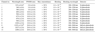
FWHM: full width at half maximum. a 315 nm channel is not used by JMA/MRI. b 1225 nm channel is used by JMA/ MRI.
In this study, measurements were conducted using two POM-02 sky radiometers that are used by the Japan Meteorological Agency/Meteorological Research Institute (JMA/MRI). One is used as a calibration reference, POM-02 (calibration reference), and the other is used for continuous measurement at the Tsukuba MRI observation site, POM-02 (Tsukuba). In Table 1, the nominal specifications of the filters are shown. The JMA/MRI does not use the 315 nm channel because the transmittance of the lens was low at this wavelength. Instead, the JMA/MRI added a 1225 nm channel. The sensor output in the file storing the measurement values of POM-02 is the current: the unit is ampere (A). Therefore, the unit of the calibration constant in this paper is ampere (A).
To calibrate the reference POM-02 by the normal Langley method (i.e., the same air mass of air molecule scattering for all attenuating substances, see Sect. 4.1), the measurements were conducted at the NOAA Mauna Loa Observatory (MLO) for about one month every year, for more than 20 years. The MLO (19.5362∘ N, 155.5763∘ W) is located at an elevation of 3397.0 m amsl on the northern slope of Mauna Loa, Island of Hawaii, Hawaii, USA. The atmospheric pressure is about 680 hPa. The MLO is one of the most suitable places to obtain data for a Langley plot (Shaw, 1983) and for a solar disk scan. Using these data, the calibration constant is estimated and the SVA is calculated.
The continuous observation was performed at the JMA/MRI (36.05∘ N, 140.13∘ E) in Tsukuba, which is located about 50 km northeast of Tokyo. Using these continuous measurement data, the calibration constants for the IML method were calculated using the SKYRAD software package (Nakajima et al., 1996, OpenCLASTR, http://www.ccsr.u-tokyo.ac.jp/~clastr/, last access: 18 September 2018). Usually, the calibration of POM-02 for continuous measurement is conducted by comparison with the side-by-side measurement data from the reference POM-02.
The temperature dependence of the sensor output was measured using the same equipment that was originally used to measure the temperature dependence of the pyranometer. This equipment is managed and maintained by a branch of the JMA Observation Department. The main components of this equipment are a temperature-controlled chamber, light source, and stabilized power supply.
The measurements for investigating the temperature characteristics of POM-02 were made as follows.
To stabilize the equipment, the power supply of the equipment was turned on the day before the measurement date. On the measurement day, the light source was first turned on, then the temperature was varied every 90 min, and the temperature and output from POM-02 were recorded continuously. The temperature was set to 40, 20, 0, −20, 0, 20, 40, and 20 ∘C. It took about 30 (40) min after increasing (decreasing) the temperature for the temperature and the output of POM-02 to become stable. Temperature characteristics were investigated using data between 70 and 90 min after varying the temperature.
To check the stability of the equipment, the staff of the JMA recorded the output of the pyranometer CMP-22 (Kipp & Zonen, Netherland) continuously for 11 h at a temperature setting of 20 ∘C. As a result, the variation of the hourly mean values of the output was within ±0.05 %.
The temperature correction was performed for each individual measurement value. The temperature dependence of the sensor output was approximated by the following equation:
where V(T) is the sensor output at temperature T, V(T=Tr) is the sensor output at reference temperature Tr, and coefficients C1 and C2 were determined by the least squares method. In the case of POM-02, the sensor output is current, and the unit is ampere (A). Therefore, the measured V(T) is corrected using Eq. (1).
In this section, the temperature characteristics of the POM-02 are described. The POM-02 is temperature-controlled; however, the temperature control is insufficient. Therefore, the sensor output of the POM-02 is dependent on the environmental temperature.
The purpose of the temperature control is to keep the temperature inside the instrument from decreasing to below levels that will reduce the instrument's precision. Instruments are designed to activate the heater when the inside temperature is less than 20 or 30 ∘C. For colder regions, such as polar regions, the minimum temperature threshold for activating the heater is 20 ∘C, and in other regions the threshold is 30 ∘C. When the temperature near the rotating filter wheel inside the instrument is below the threshold temperature (20 or 30 ∘C), the instrument is heated. When the temperature exceeds the threshold, heating is stopped. However, there is no cooling mechanism for when the temperature inside the instrument is higher than its threshold temperature. To monitor the temperature inside the instrument, a temperature sensor is attached near the rotating filter wheel. Furthermore, the shortwave-infrared detector, which is thermoelectrically cooled, is equipped with a temperature sensor and temperature data can be recorded.
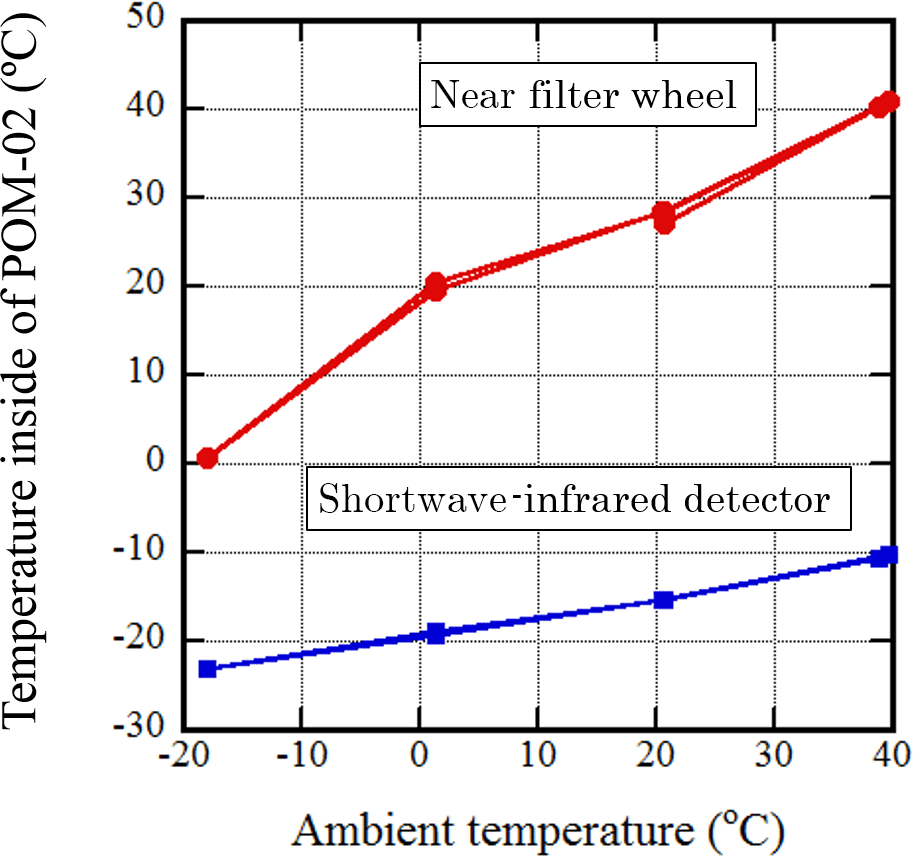
Figure 1Relation between the inside temperatures of the instrument and the ambient environmental temperature for POM-02 (calibration reference).
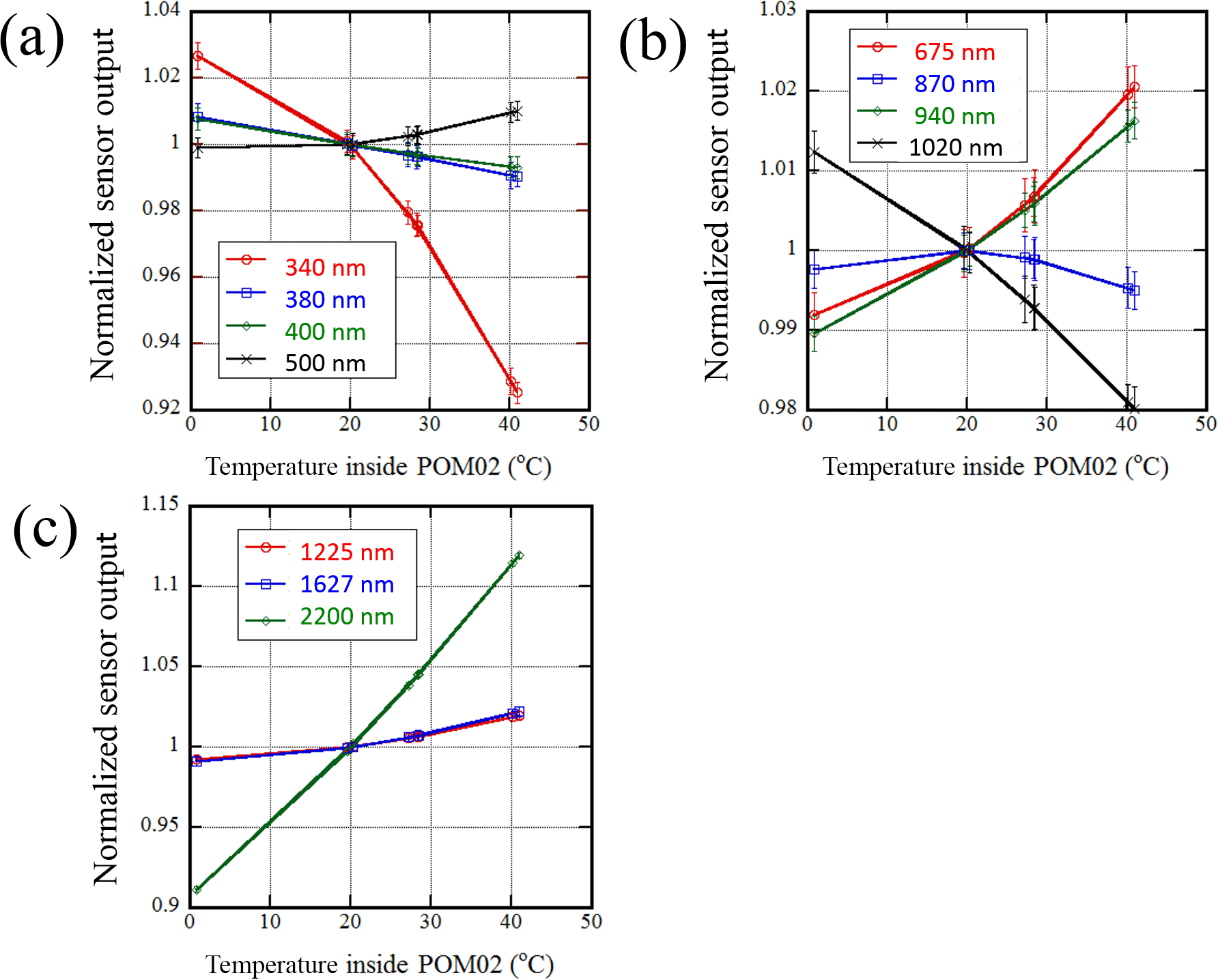
Figure 2Relation between the sensor output and the inside temperature near the filter wheel for POM-02 (calibration reference). The sensor output is normalized by the output at 20 ∘C. The error bars are the standard deviation. Panel (a) represents 340, 380, 400, and 500 nm. Panel (b) represents 675, 870, 940, and 1020 nm. Panel (c) represents 1225, 1627, and 2200 nm.
In Fig. 1, an example of the relation between the temperature near the rotating filter wheel and the environmental temperature for POM-02 (calibration reference) is shown. The red line is the temperature near the rotating filter wheel that holds the individual filters and the blue line is the temperature of the shortwave-infrared detector. The temperature control setting of this POM-02 is 20 ∘C. As heat is generated from the electric circuit inside the POM-02, the inside temperature exceeds 20 ∘C even if the ambient temperature is less than 20 ∘C. The heater stops when the inside temperature of the POM-02 exceeds 20 ∘C. However, as there is no cooling mechanism, the temperature inside the POM-02 rises as the ambient temperature increases. When the ambient temperature is very low, the temperature does not rise to 20 ∘C because the heater is not powerful enough. For example, when the ambient temperature was about −20 ∘C, the internal temperature was about 0 ∘C. The ambient temperature was varied in the order of 40, 20, 0, −20, 0, 20, 40, and 20 ∘C. As the mounting position of the temperature sensor and the thermal structure of the instrument were different for each product, not every POM-02 temperature responds in the same way.
In Fig. 2, the relation between the sensor output and the inside temperature near the filter wheel for POM-02 (calibration reference) is shown. The sensor output is normalized by the sensor output at 20 ∘C. The ambient environmental temperature was varied from −20 to 40 ∘C. The detector used for wavelengths shorter than 1020 nm was a Si photodiode, and the detector for the 1225, 1627, and 2200 nm wavelengths was a thermoelectrically cooled InGaAs photodiode. In this study, the former wavelength region is referred to as the “visible and near-infrared region” and the latter is the “shortwave-infrared region”.
The temperature dependence of the sensor output in the 340 and 2200 nm channels was larger than in the other channels. The range of the atmospheric temperature at Tsukuba was about −5 to 35 ∘C (the range of the monthly mean temperature was 2.7 to 25.5 ∘C), and the resulting inside temperatures were between 15 and 35 ∘C (Fig. 1), and the change in the instrument response was less than 1.5 %, except for the 340 and 2200 nm channels. The temperature dependence of the sensor output varies with the channel.
In the 340 nm channel, the sensor output decreased by 7 % when the internal temperature increased from 20 to 40 ∘C. In the 2200 nm channel, the sensor output decreased by a rate of 5 % to 6 % per 10∘C of temperature increase. Therefore, the temperature dependence of the sensor output cannot be ignored in these two channels.
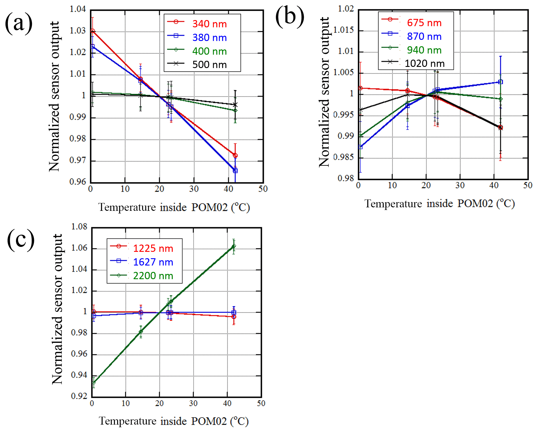
In Fig. 3, the temperature dependence of the sensor output for POM-02 (Tsukuba) is shown. The temperature dependence of the sensor output in the 380 nm and 2200 nm channels for this POM-02 are larger and smaller, respectively, than that for the calibration reference POM-02. In the 340 and 380 nm channels, the rate of sensor output decrease was about 1.5 % per 10∘C, and in the 2200 nm channel, the rate of sensor output decrease was about 3 % per 10∘C. In the other channels, the temperature dependence of the sensor output was less than 1 % for temperatures between 0 and 40 ∘C.
The temperature dependence of the detector sensitivity, as shown in the specifications data sheet of the detector (https://www.hamamatsu.com/resources/pdf/ssd/s1336_series_kspd1022e.pdf, last access: 18 September 2018) is almost zero, i.e., indistinguishable from zero in the sensitivity diagram, at wavelengths from 300 to 950 nm. At a wavelength of 1020 nm, it is about 0.2 % per ∘C. At wavelengths of 1225, 1627, and 2200 nm, they are almost zero, −0.05 % per degree, and 0.02 % per ∘C, respectively (https://www.hamamatsu.com/resources/pdf/ssd/g12183_series_kird1119e.pdf, last access: 18 September 2018). The temperature dependencies of the sensor output shown in Figs. 2 and 3 are characteristic of the entire instrument. Some channels exhibit greater temperature dependence than the temperature dependence of the detector.
Though only two examples were shown here, the temperature dependence of the sensor output differed between instruments. If we want to determine the temperature dependence of the sensor output precisely, we need to measure it for each instrument or only use channels with a small temperature dependence.
In this section, the Langley method is briefly reviewed and the Langley method used in this study is described. Before investigating the RMSE of the IML method, first the precision of the normal Langley method and the transfer of the calibration constant are investigated. The transferred calibration constant can be obtained by comparing side by side measurements of the direct solar irradiance.
4.1 Brief review of Langley method
According to the Beer–Lambert–Bouguer attenuation law, the directly transmitted monochromatic solar irradiance F(λ) at wavelength λ is as follows:
where F0(λ) is the monochromatic solar irradiance at wavelength λ, at the mean earth–sun distance (1 AU), R is the earth–sun distance in AU, and k(λ,s) is the total spectral extinction coefficient at position s. The integral of k(λ,s) is the optical path length, and the integration is done along the path of the solar beam. In Eq. (2), several atmospheric components contribute to k(λ,s): Rayleigh scattering by air molecules, extinction by aerosol and cloud particles, absorbing gas such as water vapor and ozone, etc.
When the extinction coefficient is composed of several components, Eq. (2) becomes
Introducing the vertical optical thickness (or optical depth) for each component provides the following equation:
where the extinction coefficient for the ith component is integrated in the vertical direction (Liou, 2002).
Using the optical depth τi(λ), the optical path length is written as follows:
where mi(θ) is the air mass for the ith component, and θ is the solar zenith angle. The air mass varies with the solar zenith angle, and for small θ may be approximated by 1∕cos(θ). For large zenith angles (, the sphericity and atmospheric refraction must be taken into account. As mi(θ) also depends on the vertical distribution of a component, mi(θ) is different for each component.
Substituting Eq. (5) into Eq. (3) gives the following equation:
Traditionally, the directly transmitted solar irradiance is represented as follows:
where mT(θ) is the total air mass and τT(λ) is the total optical depth.
To obtain a measurable radiometer signal, F(λ) is measured with some small but non-zero finite bandwidth at the selected wavelength and finite field of view (Shaw, 1982). Spectral filter radiometers with a bandwidth of about 10 nm or less in the visible and near infrared region were recommended and used for accurate measurements (Shaw, 1976, 1982; Reagan et al., 1986; Bruegge et al., 1992; Schmid and Wehrli, 1995; Holben et al., 1998; Kazadzis et al., 2017).
The solar direct irradiance spectrally averaged by the spectral response function is written as follows:
where is the solar direct irradiance spectrally averaged at the center wavelength λ0, and φ(λ) is the filter response function.
As the wavelength dependence of the molecular scattering coefficient, extinction coefficient by aerosols, and continuous absorption coefficient by gas are small, these values are approximated by the value at the center wavelength λ=λ0. The extraterrestrial solar irradiance is approximated by the filter-weighted value. However, in the gas absorption band composed of many absorption lines, such as the 940 nm channel, the filter-weighted transmittance does not follow the Beer–Lambert–Bouguer attenuation law,
where
and τgas is the optical depth of the gas absorption lines.
When estimating the optical depth of the aerosol from measurement of the direct solar irradiance, the wavelength range where the absorption by gas is as small as possible is chosen (Shaw, 1982). When estimating the precipitable water vapor, a wavelength range of 940 nm is often chosen.
Considering molecular scattering, absorption by ozone (Chappuis bands, Huggins bands), extinction by aerosol, and absorption by gas absorption lines, Eq. (9) becomes as follows:
where mR, , and maer are the air mass for molecular scattering (Rayleigh scattering), ozone, and aerosol, respectively, and τR, , and τaer are the optical depths for molecular scattering, ozone, and aerosol, respectively.
If the sensor output is proportional to the input energy, the following equation can be written.
Here, the contribution of the diffuse radiances in the FOV is neglected.
If absorption by gas absorption lines can be ignored, Eq. (12) can be written as follows:
Taking the logarithm of Eq. (13) leads to
If a series of measurements is taken over a range of mT(θ), during which the optical depth τT(λ0) remains constant, may be determined from the ordinate intercept of a least squares fit when one plots the left-hand side of Eq. (14) vs. mT(θ). This procedure is commonly known as the Langley-plot calibration. is the sensor output for the extraterrestrial solar irradiance at 1 AU earth–sun distance, and is called the calibration constant.
The Langley method, which is performed assuming the same air mass of air molecule scattering for all attenuating substances is sometimes called the normal Langley method (Reagan et al., 1986) or the traditional Langley method (Schmid and Wehrli, 1995). In this paper, “normal Langley” is used.
When the different components contributing to the attenuation have different vertical distributions, each component has a different dependence of the air mass on the solar zenith angle. In the refined Langley method, the contribution to the attenuation of each component is treated separately (Thomason et al., 1983; Guzzi et al., 1985; Reagan et al., 1986; Bruegge et al., 1992; Schmid and Wehrli, 1995).
The effect of the vertical distribution of ozone on the determination of the calibration constant was examined by Thomason et al. (1983). According to their results, the influence of the vertical distribution of ozone is large when 0.1 % accuracy is required, but at a wavelength of 500 nm, the error is at most 0.1 %, even if using the air mass of the uniform mixture atmosphere.
The presence of thick stratospheric aerosol layers, such as those measured immediately after major volcanic eruptions including the Pinatubo eruption in July 1991, may cause the air mass to be different from under ordinary conditions (Russell et al., 1993; Dutton et al., 1994).
For the water vapor absorption band at a wavelength of 940 nm, the Beer–Lambert–Bouguer law is not valid. In this region, the modified Langley method is often used (Reagan et al., 1987a; Bruegge et al., 1992; Schmid and Wehrli 1995). In the modified Langley method, the transmittance is approximated by an empirical formula. In Sect. 7, this modified Langley method is applied to the on-site measurement data.
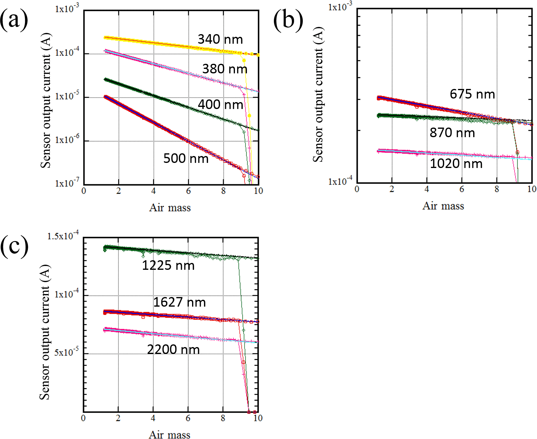
Figure 4Examples of Langley plots using the data obtained at MLO, on 3 November 2015. The sensor output of POM-02 is current: the unit is ampere (A).
4.2 Normal Langley method
In this section, the precision of the normal Langley is investigated,
where maer(θ) is approximated by mR(θ). mR(θ) is calculated using the formula from Kasten and Young (1989). To compute maer(θ) exactly, we would need a vertical profile of the aerosol extinction coefficient; however, it is difficult to obtain the vertical profile of the aerosol extinction coefficient. Therefore, mR(θ) is often used instead of maer(θ) (Schmid and Wehrli, 1995; Holben et al., 1998).
In the case of “no gas absorption”, the following equation is used:
where mT(θ)=mR(θ); the same air mass is assumed for all attenuators.
Although the term for the gas line absorption is not written explicitly, when the line absorption is in the region of the weak line limit, the absorptance ( transmittance) is proportional to the sum of the line absorption strengths. Therefore, the transmittance changes exponentially with the air mass.
In the case of “gas absorption”, the following equation is used:
When calculating , the absorption of water vapor, carbon dioxide, ozone, methane, carbon monoxide, and oxygen is only taken into consideration when the absorptions by these gases are in the range of the response function.
Table 2Example of calibration constants (V0) determined by using the data taken at MLO.
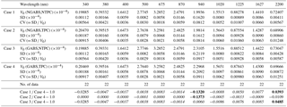
Bold: ABS(ERR) > 0.03; italic:
ABS(ERR) < 0.01; V0: mean value of calibration constant in 2015 MLO
observation (the unit of V0 is ampere(A)); SD: standard deviation; CV:
coefficient of variation
or relative standard deviation
(= SD ∕ V0); GABS: consideration of gas absorption; NGABS: no
consideration of gas absorption; TPC: consideration of temperature
correction; NTPC: no consideration
of temperature
correction.
It is recommended that the measurements for calibration by the Langley method be conducted at a high mountain observatory. The MLO is one of the most suitable places to make measurements for calibration by the Langley method. Though the air at MLO is exceedingly transparent, it is affected in late morning and afternoon hours by marine aerosol that reaches the observatory during the marine inversion boundary layer breakdown under solar heating. Typically, by late morning, the downslope winds change to upslope winds, which bring moisture and aerosol-rich marine boundary layer air up the mountainside, resulting in an abundance of orographic clouds at the observatory (Shaw, 1983; Perry et al., 1999). Therefore, using data taken in the morning is recommended and used (Shaw, 1982; Dutton et al., 1994; Holben et al., 1998).
In AERONET, the variability of the determined calibration coefficient as measured by the coefficient of variation or the relative standard deviation (CV or RSD, standard deviation/mean) is ∼0.25–0.50 % for the visible and near-infrared wavelengths, ∼0.5–2 % for ultraviolet and ∼1–3 % for the water vapor channel (Holben et al., 1998).
In this study, though using data taken in the morning is recommended, both morning and afternoon data were used for the Langley plot. Our observation period for calibration by the Langley method is short, about 1 month, so we want to use all the data effectively. Furthermore, the quality of the Langley plot can be checked by an analysis of the residuals; for acceptable data, no trend or systematic pattern is visible when the residuals vs. air mass are plotted. The residuals were carefully checked and most results for the afternoon data were not included in the analysis.
Figure 4 shows an example of a Langley plot using the data obtained at MLO. In these Langley plots, the data in both the morning and afternoon are plotted. The linear regression lines were determined using the data with an air mass range between 2 and 6, in the morning. In these examples, the data in the afternoon lies close to the regression line fitted to the morning data. On such days, the Langley plot was also applied to the afternoon data. From these examples, by using data taken at a location with suitable conditions, it is possible to determine a precise calibration line.
At MLO, 10 to 20 measurements for the Langley calibration can usually be taken over a period of 30 to 40 continuous observation days depending on the weather conditions. Shortwave-infrared channels (1225, 1627, and 2200 nm) are more sensitive to weather conditions than channels in the visible and near-infrared range, because there are water vapor absorption bands in the shortwave-infrared channel and the water vapor in the atmosphere tends to fluctuate.
Table 2 shows the calibration constants (V0) determined using the data taken from October 2015 to November 2015 at MLO. The calibration constants were calculated for the following four cases:
-
Case 1 – no gas absorption, and no temperature correction (NGABS, NTPC);
-
Case 2 – no gas absorption, and temperature correction (NGABS, TPC);
-
Case 3 – gas absorption, and no temperature correction (GABS, NTPC);
-
Case 4 – gas absorption, and temperature correction (GABS, TPC).
The CV of the calibration constants (SD∕V0, SD is the standard deviation, V0 is the mean) were 0.2 % to 1.3 % except in the 940 nm channel, where the mean V0 and standard deviation were calculated from all data with weighting. The weight is calculated from the RMSE of the regression line and the observations (see Appendix A). From these results, it can be seen that the calibration constant can be reliably determined by the normal Langley method, using the data taken at MLO. In AERONET, similar results were obtained (Holben et al., 1998).
Based on the ratio of Case 3 ∕ Case 4, the effect of the temperature dependence on the 340 and 2200 nm channels was about 3 % and 5 %, respectively. In the other channels, the effect of the temperature dependence is less than 0.9 %. The range of the atmospheric temperature was about 5 to 15 ∘C when the measurements for the calibration at MLO were conducted. Therefore, the effect of the temperature dependence on the sensor output is small.
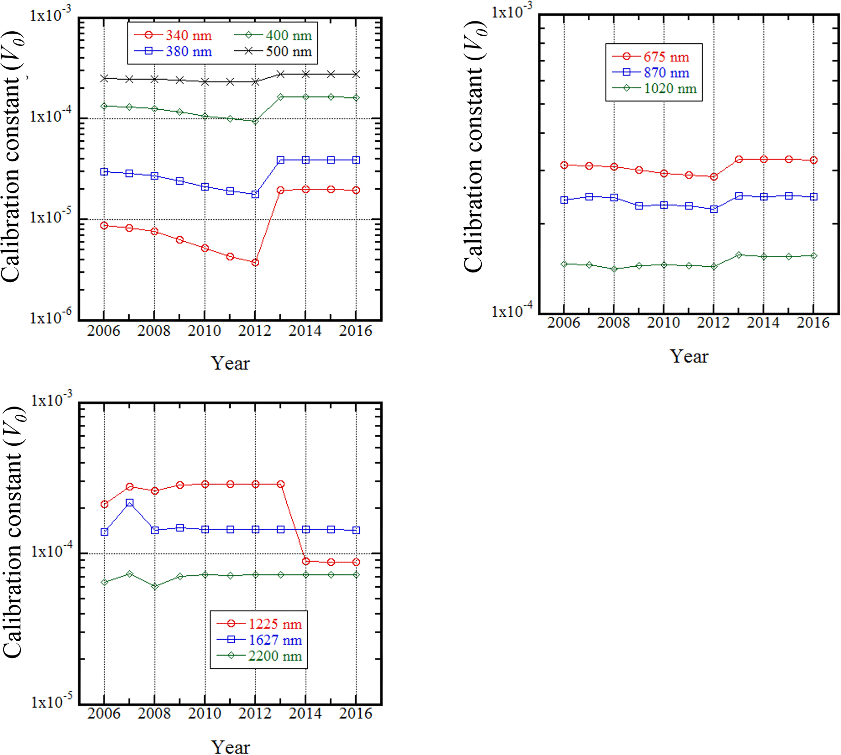
Figure 5Annual variation of the calibration constants (V0) for POM-02 (calibration reference). The sensor output of POM-02 is current. The unit of V0 is ampere (A).
From the ratio of Case 2 ∕ Case 4, the effect of the gas absorption is more than 10 % in the 940 nm channel, less than 0.4 % in the 1225 and 1627 nm channels, and about 1 % in the 2200 nm channel. These channels have weak gas absorption by water vapor, CO2, and CO.
As seen from the ratio of Case 1 ∕ Case 4, the calibration constants, except in the 340, 940, and 2200 nm channels, can be determined with a difference of less than 1 % without consideration of the temperature effect and gas absorption by using the data taken at MLO.
The results shown here were obtained using the data taken at MLO.
To calibrate the 940 nm channel, the vertical distribution of water vapor is necessary. The vertical distribution of water vapor is constructed with radiosonde data from the nearest site, precipitable water vapor (PWV) by the Global Positioning System (GPS), and the relative humidity is measured at MLO, and the transmittance is calculated as in Uchiyama et al. (2014). The radiosonde measurements were taken twice a day, and the PWV by GPS were the 30 min averages. The temporal resolution of these data is not high enough to precisely determine the vertical distribution of the water vapor, resulting in a large error in the calibration constant in the 940 nm channel.
Figure 5 shows the annual multi-year variation of the calibration constants (V0) for POM-02 (calibration reference). The lens in the visible and near-infrared region (Si photodiode region) was replaced in 2013 and the interference filter in the 1225 nm channel was replaced in 2014. As insufficient data were taken due to bad weather conditions in 2007 and 2008, the calibration could not be performed with sufficient precision. Therefore, the degradation is not smooth in some channels.
In general, the degradation at shorter wavelengths is larger than at longer wavelengths in the Si photodiode region. During the period from 2006 to 2012, the changes of V0 in the 340, 380, and 400 nm channels were −10 % per year, −7 % per year, and −4 % per year, respectively. The changes of V0 in the 500, 675, and 870 nm channels were about −1 % per year, and that in the 1020 nm channel was almost zero. These results indicate that calibration is necessary at least once a year to monitor the degradation of V0. After replacing the lens in 2013, the degradation of the 340, and 380 nm channels became smaller. The manufacturer of the sky radiometer may have upgraded the lens.
Table 3Results of the calibration constant transferred from POM-02 (calibration reference) to POM-02 (Tsukuba) and POM-02 (Fukuoka) in December 2014.
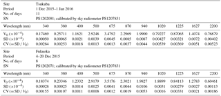
V0: mean value; SD: standard deviation; CV: coefficient of variation or relative standard deviation (= SD ∕ V0).
The calibration in the shortwave-infrared channels (1225, 1627, and 220 nm) is sensitive to weather conditions. Therefore, the interannual variation of the calibration constants in these channels is not always smooth. However, from 2009 to 2016, the annual change of the calibration constant in the shortwave-infrared channels was less than 1 %.
4.3 V0 calibration transfer by direct solar measurement
The calibration constant for one instrument can be used to estimate the calibration constant for another instrument by comparison with the simultaneous measurements of the solar direct irradiance.
The measurements for the comparison were made every minute using the same data acquisition system. It takes about 10 s to measure 11 channels at each time. Measurements by all POM-02 are done at the same time. The calibration of time is carried out every hour using the NTP (Network Time Protocol) server. For data comparison, only air mass data less than 2.5 were used on clear days. The comparisons were made under the assumption that the filter response functions of POM-02 are the same. When there is a difference in the filter, the relationship between the outputs of both becomes nonlinear. When this greatly deviated from the linear relationship, the characteristics of either filter had changed, and it is necessary to replace the filter.
Table 3 shows the results of the calibration constant transferred from POM-02 (calibration reference) to POM-02 (Tsukuba) and POM-02 (Fukuoka) in December 2014. The comparison measurements were conducted over 11 days for POM-02 (Tsukuba) and 8 days for POM-02 (Fukuoka). The CV (SD∕V0) is 0.1 % to 0.5 % depending on the wavelength, where mean V0 is the arithmetic mean. The CV is 0.5 % even for water vapor in the 940 nm channel; usually the fluctuation of the sensor output is large due to fluctuations in the water vapor amount. If the weighted mean is used as the expected value, a smaller CV than that of the arithmetic mean is expected.
The observations for the comparison depend on the weather conditions, but if there are calibrated instruments, it is the most straightforward and accurate way to transfer and determine the calibration constant for different instruments.
The JMA routine observation branch participated in the Fourth WMO Filter Radiometer Comparison in Davos, Switzerland, between 28 September and 16 October 2015 (Kazadzis et al., 2018). The calibration constant of POM-02 used by them was transferred from the POM-02 (calibration reference) in this study by the method shown in this paper. In this inter-comparison campaign, the aerosol optical depths at the 500 and 875 nm wavelengths were compared. The results of the comparison showed that the JMA's POM-02 met the World Meteorological Organization (WMO) criterion (WMO, 2005). This shows that the method shown in this study is adequate. The WMO criterion for the absolute differences of all instruments compared to the reference is defined as follows: “95 % of the measured data has to be within ” (where m is the air mass).
5.1 Brief review of improved Langley method
In this section, the improved Langley method is briefly reviewed.
The solar direct irradiance at the surface normal to the solar beam based on the Beer–Lambert–Bouguer Law is written as follows:
where F and F0 are the solar irradiance at the surface and the top of the atmosphere, respectively, R is the earth–sun distance in astronomical units (AUs), is the air mass, μ0 is the cosine of the solar zenith angle, and τ is the total atmospheric optical depth.
The single scattered radiance by aerosol and molecules in the almucantar of the sun is given by the following equation (Tanaka et al., 1986):
where a one-layer plane-parallel atmosphere is assumed, τsca=τω0 is the layer scattering optical depth, ϕ is the azimuthal angle measured from the solar principal plane, ω0 is the single scattering albedo, and P(cosΘ) is the normalized phase function at the scattering angle Θ. The improved Langley method is based on these equations.
If the sensor output is proportional to the input energy, the sensor output for the direct solar measurement can be written as follows:
where V=CF, V0=CF0, and C is the proportional constant (sensitivity). The contribution of scattered light in the field of view is neglected.
The sensor output for the measured single scattering V1 can be written as follows:
where ΔΩ is the SVA.
From these equations, the following equations can be obtained:
Then from Eq. (20), we get the following equations:
If m, mτ, and mτsca can be obtained, the logarithm of the sensor output can be linearly fitted with m, mτ, and mτsca. The case when the x axis is m and the y axis is lnVR2 corresponds to the normal Langley method, and the case when the x axis is mτ or mτsca and the y axis is lnVR2 is the improved Langley method. In the normal Langley method, the intersection of the y axis and the regression line is lnV0 and the slope of the regression line is −τ. There are two IML methods. If the x axis is mτ, the intersection of the y axis and the regression line is lnV0 and the slope is −1. Otherwise, when the x axis is mτsca, the intersection of the y axis and the regression line is lnV0 and the slope is . The SKYRAD package adopts the latter method.
In the SKYRAD package, two observable quantities are analyzed. One is the direct solar irradiance (Eq. 20), and the other is defined as follows:
where V(λ,Θ) is the sensor output of the sky radiance measurement for the scattering angle Θ, , ΔΩ is the SVA of the sky radiometer, and V(λ,0) is the radiometer output due to direct solar irradiance. This is the sky radiance normalized by the direct solar irradiance.
V(λ,Θ) is composed of the single scattering and multiple scattering radiances.
Therefore, Eq. (25) can be expressed as follows:
where Rm(λ,Θ) is the contribution of multiple scattering.

Figure 6Monthly mean values and standard deviation of the inside temperature of POM-02 (Tsukuba) (blue line) and the temperature of the shortwave-infrared detector (red line) from December 2013 to December 2016.
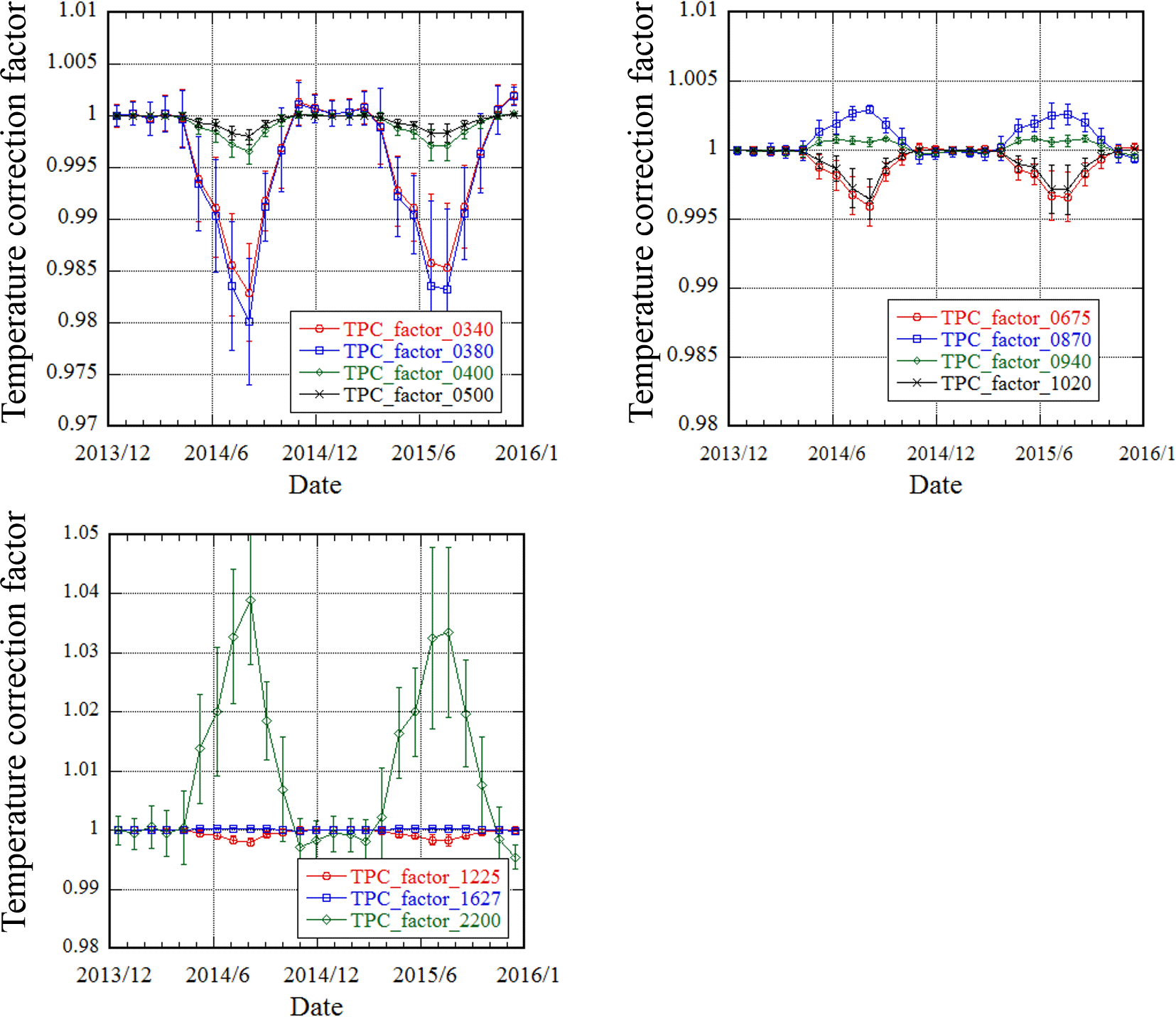
Figure 7Monthly means of the temperature correction factors and standard deviation for POM-02 (Tsukuba) from December 2013 to December 2016.
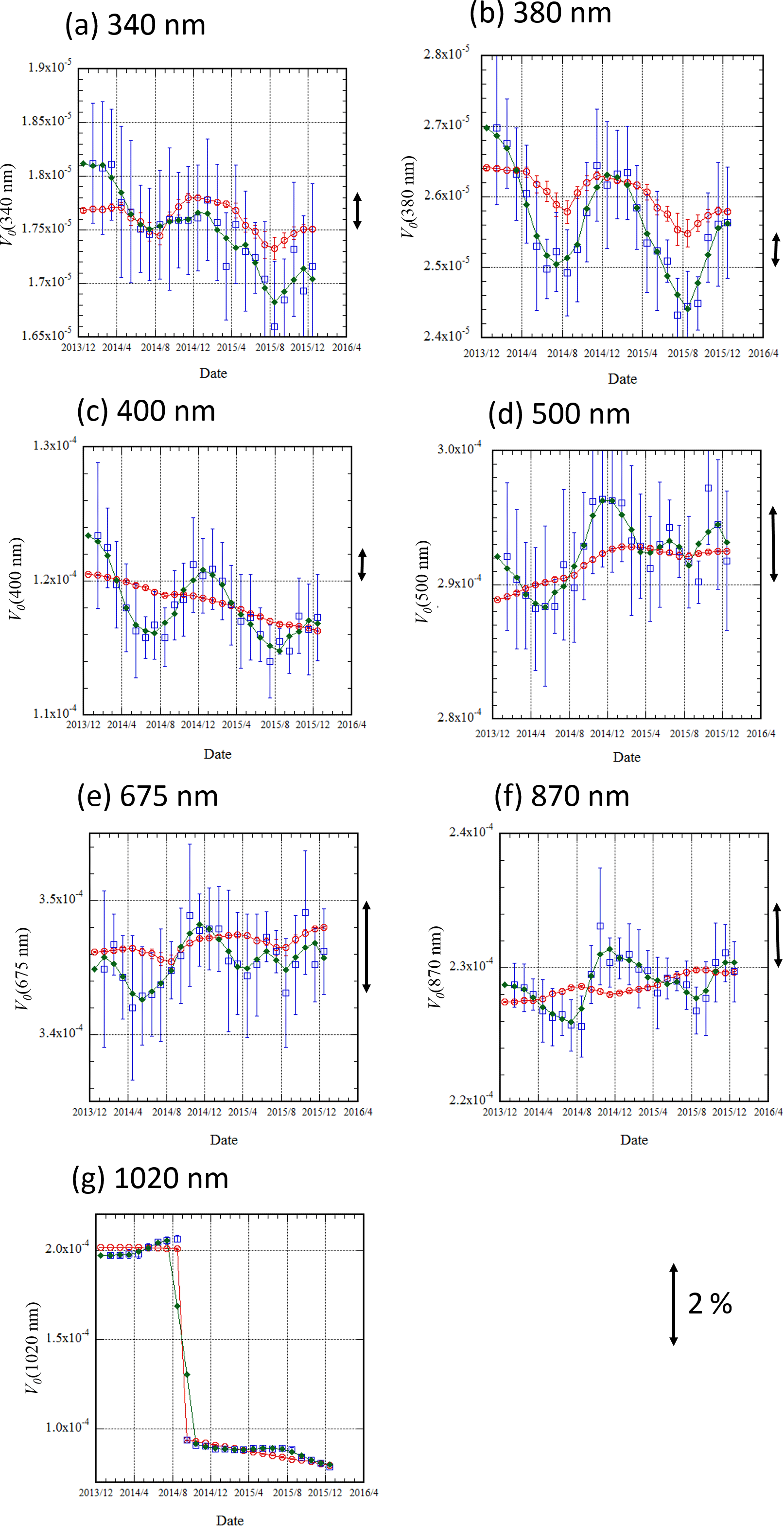
Figure 8Time series of the calibration constant for POM-02 (Tsukuba) from January 2014 to December 2015. Blue open squares with error bars denote the calibration constants determined by the IML method. The green line shows the three-point running mean of IML, and the red line is the calibration constant interpolated from calibration constants transferred from POM-02 (calibration reference). The unit of V0 is ampere (A). A double-headed arrow shows 2 % width. A 2 % scale arrow is not shown in the case of (g) 1020 nm.
In the SKYRAD package, given the initial value of the column particle volume size distribution (dV∕dlogr) and the complex refractive indexes, τ, P(cosΘ), and ω0, are calculated assuming the spherical homogeneous particle. On the basis of these single scattering properties, the multiple scattering term (second term on the right side) in Eq. (26) is evaluated, and the single scattering term (first term on the right side) in Eq. (26) can be obtained. The new dV∕dlogr is retrieved from the single scattering term in Eq. (26) by the inversion scheme. Using the retrieved dV∕dlogr, τ, P(cosΘ), and ω0 are calculated, and the observed values are reconstructed, and then the error is calculated. Until the error satisfies the convergence condition, the above procedure is iterated. In the above procedure, the complex refractive indexes for each channel are fixed and the measurement data with a scattering angle of less than 30∘ are used.
Once mτ is obtained, the calibration constants can be estimated from . However, in the SKYRAD package, lnV0 is determined from . Comparing this equation with Eq. (24), W0 must be the single scattering albedo. The single scattering albedo is defined as the ratio of the scattering coefficient to the extinction coefficient. Therefore, the single scattering albedo must be a value between 0 and 1. However, W0 is frequently greater than 1. Therefore, it is treated as a constant in the estimation of lnV0. To distinguish between ω0 and W0, W0 was used. The fitted error, number of measurements, and the transmittance are checked. Then, the data passing the check criterion are chosen as the calibration constants.
5.2 Comparison between improved Langley and normal Langley method
In the improved Langley (IML) method, the temperature dependence of the sensor output is not usually explicitly considered. This means that the calibration constant determined by the IML method implicitly includes the temperature dependence of the sensor output. Before comparing the calibration constant determined by the IML method and that transferred from POM-02 (calibration reference), we examined how much the sensor output changes with ambient temperature change.
In Fig. 6, the monthly mean values of the inside temperature of POM-02 (Tsukuba) and the temperature of the shortwave-infrared detector are shown. As seen from the figure, these temperatures were controlled in the period from November to April. In Fig. 7, the temperature correction factors are shown, where the reference temperature is 20 ∘C. In the summer, the sensor output must be corrected by 1.5 % to 2 % in the 340 and 380 nm channels and by 4 % in the 2200 nm channel. In the other channels, the corrections were less than 0.5 %: the temperature effect on these channels was small.
In Fig. 8, the calibration constants determined by the IML method from January 2014 to December 2015 are shown. To compare between the IML and normal Langley methods, the calibration constants interpolated from the calibration constants transferred from POM-02 (calibration reference) are also shown. The observations for the calibration transfer were conducted in December 2013, December 2014, and December 2015, and the calibration constants for POM-02 (Tsukuba) were determined. The calibration constants in other months were obtained by linear interpolation and the temperature correction factor was also taken into consideration. In Fig. 8, the running means of the monthly IML values are also shown.
For every channel, the calibration constants determined by the IML method have a seasonal variation: they are larger in the winter and smaller in the summer. The amplitude of the seasonal variation is larger than that of the temperature correction factor. Furthermore, the annual trend of the calibration constant, after removing the seasonal variation, is almost the same as the normal Langley method. Furthermore, Fig. 8 shows much higher noise of the IML method compared with calibration transfer method.
Table 4Statistics of the difference between IML method and normal Langley method.
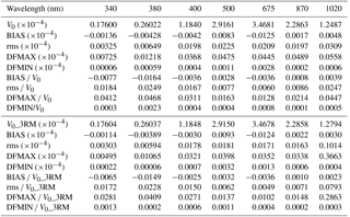
V0: mean calibration constant (IML method) from Jan. 2014 to Dec. 2015. V0_3RM: mean calibration constant (IML method, three-point running mean) from Jan 2014 to Dec 2015. BIAS: bias (mean of differences between IML and normal Langley methods). rms: root mean squares of differences between IML and normal Langley methods. DFMAX: maximum difference between IML and normal Langley methods. DFMIN: minimum difference between IML and normal Langley methods.
In the 380 nm channel, the calibration constant changes due to the temperature dependence of the sensor output: in the summer the calibration constant decreases by about 2 %. The calibration constant (V0) determined by the IML method changes by up to 6 %. Even if the effect of the temperature change is subtracted from the seasonal variation, there is a difference of about 4 % between the V0 determined by the IML method and V0 interpolated from V0, determined by inter-comparison with the POM-02 (calibration reference). In the 400, 500, 675, and 870 nm channels, there is a difference of 1 % to 2 % between the calibration coefficients, and in the 340 nm channel, there is a difference of 3 % between the calibration coefficients. In the 1020 nm channel, as the interference filter was changed in September 2014, a direct comparison is difficult. In Table 4, the statistics of the difference between both calibration coefficients are shown. The RMSE is about 0.6 % to 2.5 %, depending on the wavelength. This result is almost the same as in Campanelli et al. (2004). However, the maximum difference between both calibration coefficients was about 1.3 % to 4.7 %, and these differences are rather large. The statistics of the three-point running mean for the IML method are also shown in Table 4. The errors are a bit smaller than those for the non-smoothed values: the RMSE is about 0.5 % to 1.7 %.
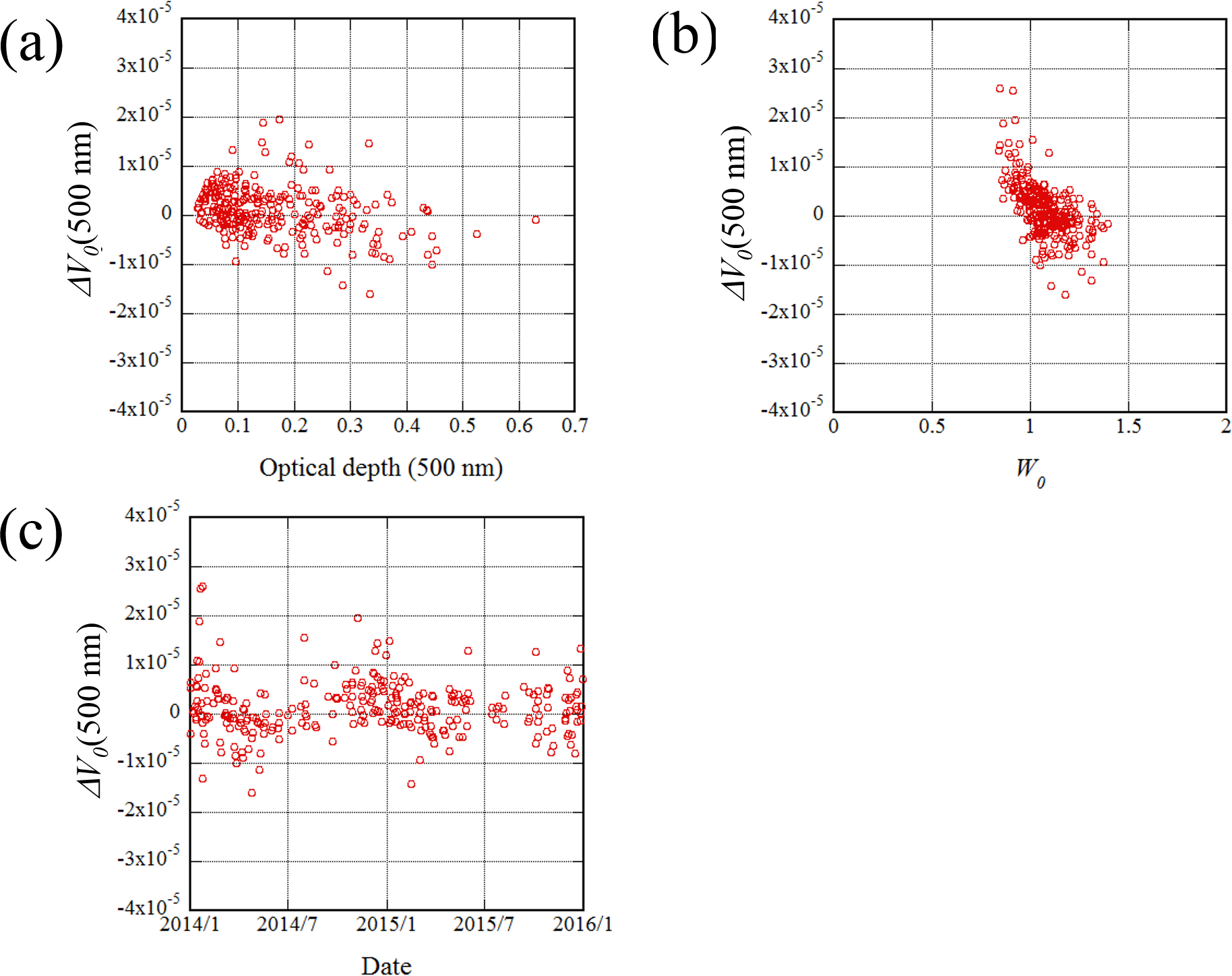
Figure 9(a) Scatter plot of ΔV0 for the 500 nm channel and the optical depth at 500 nm. (b) Scatter plot of ΔV0 and W0 for the 500 nm channel. (c) Time series of ΔV0 for the 500 nm channel from January 2014 to December 2015. ΔV0 is the difference between V0 determined by the IML method and V0 interpolated from V0, determined by inter-comparison with POM-02 (calibration reference). The unit of V0 and ΔV0 is ampere (A).
Though the period of comparison is only 2 years, the calibration constant by the IML method represents the annual trend and implicitly includes the temperature dependence of the sensor output. However, the calibration constant has a seasonal variation of 1 % to 3 %, and in some cases, the maximum difference reaches about 5 %. The 2 % error in the calibration constant is not significant in a turbid atmosphere, but it is significant in a clear atmosphere, such as in polar and ocean regions. Furthermore, there is a possibility that the seasonal variation of the calibration constant causes an artificial seasonal variation in the retrieved parameters. The seasonal variation can be reduced by smoothing, such as with a running mean. However, over-smoothing dampens the temperature effect of the sensor output.
For the 500 nm channel, Fig. 9 shows a scatter plot of ΔV0 and the optical depth at 500 nm, a scatter plot of ΔV0 and W0, and a time series of ΔV0 from January 2014 to December 2015, where ΔV0 is the difference between V0 determined by the IML method and V0 interpolated from V0 determined by inter-comparison with the POM-02 (calibration reference). In this case, the V0 values determined by the IML method with errors less than 0.01 were chosen, where the error is the root mean square difference between the observations and the fitted line. As in Fig. 8, Fig. 9c shows that ΔV0 changes seasonally.
Figure 9a shows that there is a negative correlation between ΔV0 and the optical depth; the correlation coefficient is −0.31. This result is consistent with the large amplitude of the seasonal change at short wavelengths. As a shorter wavelength usually corresponds to a thicker optical depth, a shorter wavelength corresponds to a larger amplitude of seasonal change of V0 by the IML method.
In Tsukuba, the aerosol optical depth is thicker in the summer and thinner in the winter. Therefore, the seasonal change of V0 by the IML method seems to be related to the optical thickness. However, Fig. 9b also shows that ΔV0 and W0 are negatively correlated, specifically having a correlation coefficient of −0.59, and that even if the correct W0 is determined, the ΔV0 are scattered with a width of about . As W0 is a parameter related to the single scattering albedo or refractive index, this indicates that the error depends not only on the optical depth but also on the refractive index. There is a possibility that the seasonal variation of V0 by the IML method may also be related to the seasonal variation of the refractive index.
In the current improved Langley method, the refractive index is fixed. We used (1.5, −0.001) for all wavelengths as the initial value of the refractive index when using the SKYRAD package. However, this value may not be appropriate, and the further development of the method to determine V0 while changing the refractive index is a topic for future work.
Table 5Calibration constants for POM-02 determined by using the calibrated integrating sphere measurement.
V0: calibration constant through the normal Langley method
In this section, the accuracy of the calibration using the calibrated integrating sphere is described. If POM-02 can be calibrated using the calibrated light source, then POM-02 can be calibrated quickly without being influenced by the weather.
In this study, the integrating sphere, which is calibrated and maintained by the Japanese Aerospace Exploration Agency (JAXA), was used (Yamamoto et al., 2002). This integrating sphere is used to calibrate the radiometers that are used to validate satellite remote sensing products.
To use the light source, the extraterrestrial solar irradiance, the SVA, and spectral response function of the sky radiometer are necessary, as well as the radiance emitted by the light source. The extraterrestrial solar irradiance by Gueymard (2004) was used here, along with the SVA obtained by processing the solar disk scan data.
When the integrating sphere is measured by POM-02, the sensor output is written as follows:
where Vsph(λ0) is the sensor output in channel λ0, C(λ) is the sensitivity at wavelength λ, φ(λ) is the spectral response function of the interference filter, Isph(λ) is the spectral radiance from the integrating sphere at wavelength λ, and the emitted radiance from the integrating sphere is assumed to be homogeneous. This equation is approximated as follows:
where
When the extraterrestrial solar irradiance is measured, the sensor output is written as follows:
where Vsun(λ0) is the sensor output in channel λ0, and F0(λ) is the extraterrestrial solar spectral irradiance at 1 AU. This equation is approximated as follows:
where
From Eqs. (28) and (31), Vsun(λ0) is written as follows:
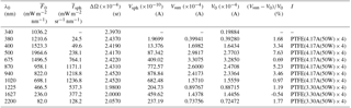
In Table 5, the calibration constants for POM-02 (calibration reference) determined from the integrating sphere measurement are compared with the results of the Langley method. At POM-02 (calibration reference), the relative difference was 0.7 % to 7.6 % in channels 2 to 8 (380 to 1020 nm), and 0.5 % to 1.8 % in channels 9 to 11 (1225, 1627, and 2200 nm). The integrating sphere used in channels 2 to 8 is different from that in channels 9 to 11.
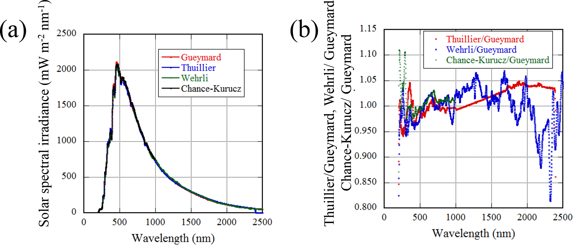
Figure 10(a) Extraterrestrial solar spectra. The value is a mean value weighted by the response function of a triangle with FWHM of 10 nm. The red line is Gueymard (2004), the blue line is Thuillier et al. (2003), the green line is Wehrli (1985), and black line is Chance and Kurucz (2010). (b) Ratios of the solar spectrum to Gueymard (2004).
The value of the extraterrestrial solar spectrum is dependent on the database. In Fig. 10, the following four data sets are shown: Thuillier et al., 2003; Gueymard, 2004; Chance and Kurucz, 2010; and the Wehrli Standard Extraterrestrial Solar Irradiance Spectrum (Wehrli, 1985; Neckel and Labs, 1981). The value is a mean value weighted by the response function of a triangle with full width at half maximum (FWHM) of 10 nm. The ratios of the solar spectrum to Gueymard (2004) are also shown. These figures show that there are several percentage points of difference in the values depending on the wavelength. The SVA uncertainty is 1 % (see Part 2, Uchiyama et al., 2018); the disk scan data were taken at MLO, where measurement conditions were good for the solar disk scan. The uncertainty of the integrating sphere was 1.7 % (Yamamoto et al., 2002). Considering the magnitude of these errors, the above differences in the calibration constants seem reasonable. However, to reduce the optical depth error below 0.01, a calibration coefficient error of several percent is too large. The calibration coefficient determined by the Langley method is better for estimating the optical depth from measurements of the direct solar irradiance. These issues were also pointed out by Shaw (1976) and Schmid and Wehrli (1995). The calibration using the standard lamp remains unchanged.
The calibration constant depends on the extraterrestrial solar irradiance in the 940 nm band, the spectral response function of the interference filter, the spectral sensitivity of the detector, and the transmittance of radiometer optics. Calibration methods for the 940 nm channel, which is in the water vapor absorption band, have been considered extensively in previous studies (Reagan et al., 1987a, b, 1995; Bruegge et al., 1992; Thome et al., 1992, 1994; Michalsky et al., 1995, 2001; Schmid et al., 1996, 2001; Shiobara et al., 1996; Halthore et al., 1997; Cachorro et al., 1998; Plana-Fattori et al., 1998, 2004; Ingold et al., 2000; Kiedron et al., 2001, 2003). For example, Uchiyama et al. (2014) developed the Langley method, which takes into account the gas absorption, and the empirical relationship between the transmittance and precipitable water vapor (PWV) was determined from the theoretical calculation using the spectral response function and the model atmosphere. The PWV is estimated from the transmittance for the 940 nm channel. The empirical formula is usually used for the transmittance of the 940 nm channel by water vapor.
Most POM-02 users have taken measurements without calibrating the 940 nm channel over a long time. To make use of these accumulated data, it is necessary to develop a calibration method using data at the observation site. Campanelli et al. (2014) developed a method to determine the calibration constant and parameters for the empirical formula of the transmittance using the on-site surface meteorological data and simultaneous POM-02 data. However, it is difficult to obtain the empirical formula for transmittance by the column water vapor from the surface measurement data.
In this study, given the spectral response function, the empirical transmittance formula is produced by the method shown in Uchiyama et al. (2014). Then, the modified Langley method shown below is performed using the empirical formula and the observation data.
The water vapor transmittance is approximated as follows:
where a and b are fitting coefficients (see Appendix B), and pwv is PWV.
The sensor output V is written as follows (Uchiyama et al., 2014):
where V0 is the calibration coefficient, R is the distance between the earth and the sun, τaer is the aerosol optical depth at 940 nm, and τR is the optical depth of the molecular scattering (Rayleigh scattering). The aerosol optical depth τaer at 940 nm is interpolated from the optical depth at 870 and 1020 nm. When interpolating τaer at 940 nm, τaer was assumed to be proportional to λ−α, where λ is the wavelength.
The above equation can be rewritten as follows:
The parameters on the left-hand side are known: V is the measurement value, R and m can be calculated from the solar zenith angle, and τR is estimated from the surface pressure. For example, R can be calculated with the simplified formula in Nagasawa (1981), m can be calculated as in Kasten and Young (1989), and τR can be calculated as in Asano et al. (1983). In the case of POM-02, the sensor output is current, and the unit of the measurement value V is ampere (A). If pwv is constant, then the right-hand side of the equation is a linear function of mb. Therefore, the values on the left-hand side can be fitted by a linear function of mb, and the intersection of the y axis and the fitted line is lnV0.
Before the above-mentioned method was applied to the MRI data, it was first applied to the data taken at MLO, which has more stable weather conditions than Tsukuba. The results applied to the data taken at MLO in October and November 2014 and in October and November 2015 are shown in Table 6.
Table 6Calibration constant at 940 nm by the modified Langley method using the data taken at MLO.
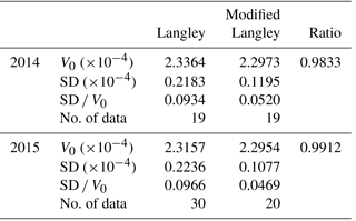
The data taken at MLO in 2014 and 2015 were used. V0: mean value; SD: standard deviation; ratio = (modified Langley V0) ∕ (Langley V0).
The calibration coefficients determined in 2014 and 2015 were A (SD ∕ V0=0.052) and A (SD ∕ V0=0.047), respectively.
The calibration coefficients determined by the Langley method with consideration of gas absorption in 2014 and 2015 were A (SD ∕ V0=0.093 and A (SD ∕ V0=0.097), respectively. Though the difference in the calibration coefficient between the Langley method with consideration of the gas absorption and the modified Langley method is 1.7 % in 2014 and 0.9 % in 2015, these calibration coefficients are very similar. The CV of the modified Langley method is smaller than the method that takes account of gas absorption more precisely than the modified Langley method. This may be due to errors in the estimates of the water vapor amount and distribution: the PWV is obtained from the GPS PWV, which has a low time resolution (30 min average), some data are missing, and the vertical distribution is estimated from only two radiosonde measurements per day near MLO.
The water vapor amount tends to fluctuate. Though the restriction that the PWV be constant is severe, the above method is applied to the data taken at Tsukuba, MRI and the calibration constants are compared with the calibration constant for POM-02 (calibration reference), which was calibrated by the Langley method, with consideration of the gas absorption, using the data taken at MLO and interpolated to the observation day (see Table 7).
The ratio of the calibration coefficients in the period of 14 December 2014 to 5 January 2015 (10 cases) was 1.0094, and in the period of 1 to 30 December 2015 (17 cases) it was 0.99818. Thus, the difference between the two methods is less than 1 %.
Although it seems that the above-mentioned modified Langley method does not work well at all locations and under all weather conditions, the calibration constant of the 940 nm channel could be determined by applying the above-mentioned method on a suitable stable and fine day at the observation site. We applied Langley method to data in the air mass range between 2 and 6. Therefore, a stable interval of 1 to 2 h is necessary. The quality of the Langley plot can be checked by an analysis of the residuals; for acceptable data, no trend or systematic pattern is visible when the residuals vs. air mass are plotted. The 940 nm channels at many observation sites have not been calibrated and are not used. The application of the modified Langley method to the on-site observation data is the next best solution.
Table 7Same as Table 6 but using the data taken at Tsukuba, MRI.
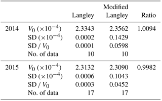
The data taken at MRI, Tsukuba in December 2014 and December 2015 were used. V0: mean value; SD: standard deviation; ratio = (modified Langley V0) ∕ (Langley V0).
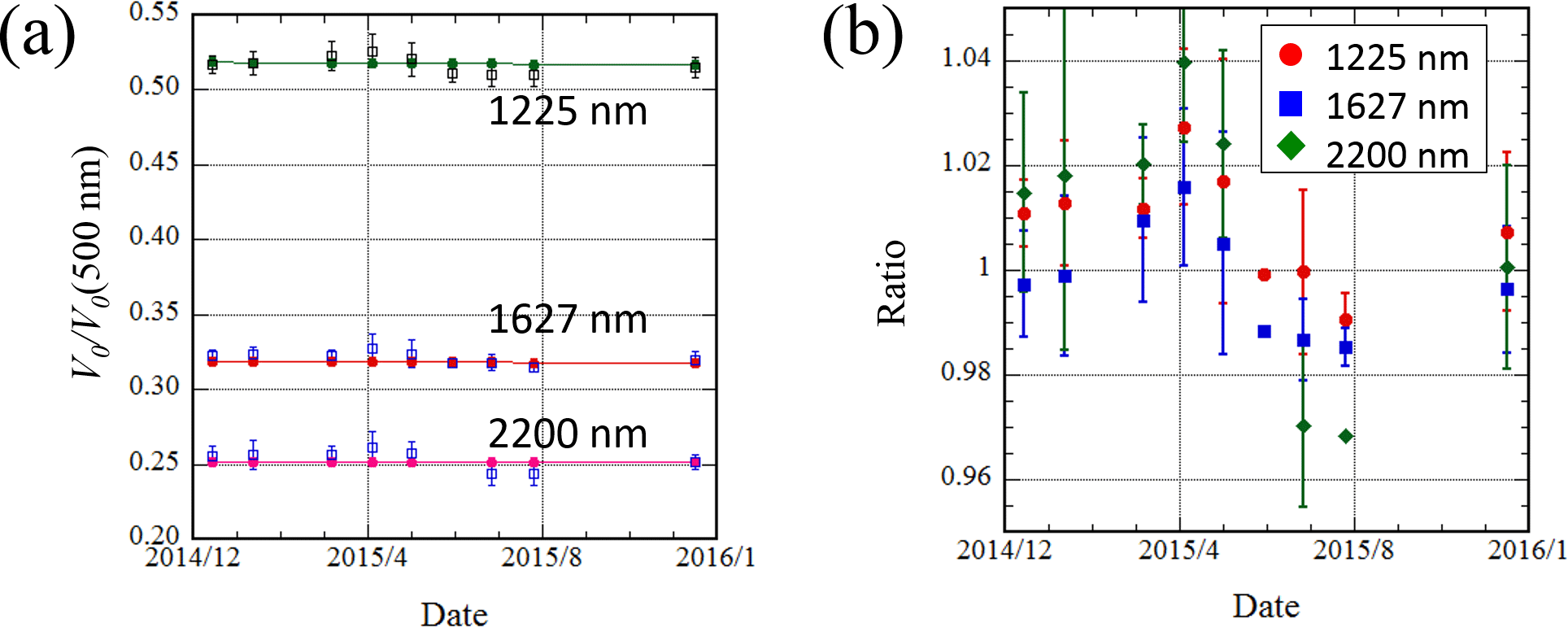
Figure 11(a) Monthly mean of V02∕V01 and the standard deviation: V01=V0(500 nm). (b) Ratio of V02 to the interpolated value of the calibration constant determined by the Langley method. The red symbols are 1225 nm, blue are 1627 nm, and green are 2200 nm.
The measurements for the shortwave-infrared channels, 1225, 1627, and 2200 nm, of POM-02 have been performed at many SKYNET sites, but the data have not been analyzed, because most POM-02 users cannot calibrate these channels by themselves.
These channels can be calibrated with the Langley method with a reasonable precision by taking into account the gas absorption. However, many users cannot make these measurements for the Langley method. Furthermore, the scattering of light in these channels is small and the IML method cannot be applied.
For some observation days, data with a very high correlation between channels may be obtained. In this case, when the calibration constant of one channel is known, then the calibration constants of the other channels can be inferred. The general method for the case when the ratio of the optical depths is constant was shown by Forgan (1994).
In this study, by assuming that the channels in the visible and near-infrared region including the 940 nm channel are calibrated, a similar method was applied to the shortwave-infrared channels to determine the calibration constant and the precision was investigated.
The sensor output of POM-02 is written as follows:
where V is the sensor output, V0 is the calibration constant, R is the distance between the earth and the sun, m is the air mass, τaer is the aerosol optical depth, τR is the optical depth of the molecular scattering (Rayleigh scattering), and Tr (gas) is the transmittance of the gas absorption.
The sensor output for channels 1 and 2 are as follows:
The calibration constant of channel 1 is assumed to be known and that of channel 2 is determined.
From Eqs. (38) and (39), the following equation is obtained:
Therefore,
If the water vapor amount is estimated from the 940 nm channel, and the mixing ratio of CO2 and CO is given, then the transmittance of gas can be estimated. Given the observation time and the latitude and longitude of the observation site, the air mass is calculated, and τR1 and τR2 are calculated from the surface pressure. Therefore, the left-hand side of Eq. (41) is known. Furthermore, when the ratio of the optical depth τ2∕τ1 is constant, then this equation is a linear function of mτ1. Therefore, the intersection of the y axis and the linearly fitted line is lnV02∕V01, and if V01 is known, then V02 is also known. Although this condition is not always satisfied, sometimes a linear fit will provide sufficient accuracy.
This method was applied to the data of POM-02 (calibration reference) from December 2014 to December 2015. The 500 nm was chosen as channel 1 in Eq. (41). The data used here had an RMSE of 0.005. In Fig. 11a, the monthly mean of V02∕V01 and the standard deviation are shown. The lines of the ratio, which are interpolated from the calibration constant determined using the data taken in October and November of 2014 and 2015 at MLO, are also shown. In Fig. 11b, the ratio of the calibration constant by the above method and the interpolated value of the calibration constant determined from MLO data are shown. In the 1627 nm channel, the differences are less than 2 % throughout the year and the differences in December and January are less than 1 %. In the 1225 nm channel, the differences are less than 2 % except in April 2015. In the 2200 nm channel, the differences in some months are more than 3 %. However, in December 2015, the differences in all channels are less than 1 %, 0.8 %, 0.4 %, and 0.1 %, respectively. This shows that the difference between the calibration constant determined by the method shown here and that determined by the Langley method is less than 1 % under suitable conditions. Currently, there is no method to calibrate the shortwave-infrared channel from on-site observation data. The method shown here is the next best solution.
Atmospheric aerosols are an important constituent of the atmosphere. Measurement networks covering an extensive area from ground and space have been developed to determine the spatiotemporal distribution of aerosols. SKYNET is a ground-based monitoring system using sky radiometers POM-01 and POM-02, manufactured by Prede Co. Ltd., Japan. To improve their measurement precision, it is important to know the characteristics of the instruments and precisely calibrate them accordingly.
There are two constants that we must determine to make accurate measurements. One is the calibration constant, and the other is the SVA of the radiometer. The calibration constant is the output of the radiometer to the extraterrestrial solar irradiance at the mean earth–sun distance (1 AU) at the reference temperature. Additionally, the temperature dependence of the sensor output is another important characteristic.
In this study, the data obtained by two sky radiometers POM-02 of the JMA/MRI are considered. One of the sky radiometers is used as a calibration reference, and the other is used for continuous measurement at the Tsukuba MRI observation site.
The sensor output of POM-02 is dependent on the environmental temperature. The temperature dependence of the sensor output in the 340, 380, and 2200 nm channels was larger than in other channels. For example, the sensor output in the 340 and 380 nm channels of POM-02 (Tsukuba) increased at a rate of about 1.5 % per 10∘C, and that in the 2200 nm channel increased at a rate of about 3 % per 10∘C. In the other channels, the sensor output increased at a rate of less than 1 % when the sensor's internal temperature was 0 to 40 ∘C. The temperature dependence of the two POM-02 examined here was different for each instrument. If we want to make accurate measurements, we need to measure the temperature dependence for each instrument or use the channels with small temperature dependences.
For the measurement at Tsukuba, the temperature inside the POM-02 (Tsukuba) was controlled during the winter and spring seasons from November to April, but was not regulated, and thus was high during the summer. In the summer, sensor output must be corrected by 1.5 % to 2 % in the 340 and 380 nm channels and by 4 % in the 2200 nm channel. In the other channels, the corrections were less than 0.5 %.
As well as determining the precision of the IML method, this study investigated the precision of the normal Langley method (i.e., the same air mass of air molecule scattering for all attenuating substances) and of the calibration transfer. From the data taken at MLO, the CV in the calibration constants determined by the normal Langley method (SD∕V0) was 0.2 % to 1.3 %, except in the 940 nm channel. The effect of gas absorption was more than 10 % in the 940 nm channel, but was less than 0.4 % in the 1225 and 1627 nm channels and less than 1 % in the 2200 nm channel, which all have weak gas absorption.
The comparison measurements for transferring the calibration constant were conducted in December at Tsukuba over about 10 days. The CV (SD∕V0) for the transfer method was 0.1 % to 0.5 %, depending on the wavelength. Though the measurements for the comparison depend on the weather conditions, when there are calibrated instruments it is a straightforward and accurate way to determine the calibration constant.
The long-term changes in the calibration constants (V0) for POM-02 (calibration reference) were also investigated. Roughly speaking, the degradation in the shorter wavelengths was larger than that in the longer wavelengths in the Si photodiode region. The changes in the 340 nm channel were −10 % per year from 2006 to 2012. After replacing the lens in 2013, the degradation of the 340 and 380 nm channels became smaller. The manufacturer of the sky radiometer may have upgraded the lens. The change in the shortwave-infrared region (thermoelectrically cooled InGaAs photodiode) was less than 1 % from 2009 to 2016. These results indicate that calibration of the instruments is necessary at least once a year to monitor the degradation of V0.
The calibration constant determined by the IML method and that transferred from the POM-02 (calibration reference) were compared using the data taken at Tsukuba from December 2013 to December 2015.
For every channel, the calibration constants determined by the IML method had a seasonal variation of 1 % to 3 %. The calibration constants determined by the IML method implicitly include the temperature dependence of the sensor output. However, even if the change due to the temperature variation is subtracted from the seasonal variation, there is a difference of 1 % to 4 % between the two calibration coefficients. The RMSEs of the differences between the two calibration coefficients were about 0.6 % to 2.5 %; this result is almost the same as that of Campanelli et al. (2004). However, in some cases, the maximum difference reached up to 5 %. Furthermore, the annual trend of the calibration constant excluding the seasonal variation was almost the same as for the normal Langley method. Furthermore, the calibration constants determined by the IML method had much higher noise than those transferred from the reference.
In order to investigate the error characteristics of the IML method, the relationship between ΔV0 and the optical depth and the relationship between ΔV0 and W0 were investigated. ΔV0 is the difference between V0 determined by the IML method and V0 interpolated from V0 determined by inter-comparison with the reference POM-02. As a result, it was found that ΔV0 and the optical depth were correlated. In Tsukuba, the aerosol optical depth changes seasonally. Therefore, the seasonal change of V0 by the IML method seems to be related to the optical depth. Furthermore, ΔV0 and W0, which are related to single scattering albedo or refractive index, were also correlated. In the current IML method, the refractive index is fixed. It is necessary to develop the proposed method to determine V0 while changing the refractive index in the future.
We also tried to determine V0 using the calibrated integrating sphere as the light source. The relative differences of V0 were about 1 % to 8 % depending on the wavelength. Considering the magnitude of the errors in the extraterrestrial solar spectrum, SVA, and the integrating sphere, the above differences in the calibration constants seem reasonable. However, to reduce the optical depth error below 0.01, an error of several percent in the calibration coefficient is too large.
The calibration method for water vapor in the 940 nm channel was considered using the on-site measurement data. V0 was determined by the modified Langley method using a pre-determined empirical transmittance equation. The differences in the calibration coefficients between the normal Langley method and the modified Langley method were less than 1 % on suitable stable and fine days.
The calibration method for the shortwave-infrared 1225, 1627, and 2200 nm channels was also considered using the on-site measurement data. It is assumed that channels in the visible and near-infrared wavelength region and the 940 nm channel are calibrated. Then, when the ratio of the optical depths between two channels is constant, the logarithm of the ratio of the sensor output can be written as a linear function of the air mass. Here, the calibration constant for one of the two channels is known and the transmittance of water vapor is calculated using the PWV estimated from the 940 nm channel. By fitting the logarithm of the ratio of sensor output to a linear function of the air mass, the ratio of the calibration constants is determined. By this method, the calibration constants could be determined within a 1 % difference from the value by the Langley method on suitable days with good weather conditions.
In this study, it is shown that some channels have a non-negligible temperature dependence in the sensor output and that the calibration constants determined by the IML method showed a seasonal variation. In channel 2 (380 nm), the maximum error reached about 5 %. Reducing the uncertainty of the IML method is a task for future work, along with the problems related to the determination of calibration constants. In particular, the calibration constants for the 940 nm channel and the shortwave-infrared channels must be determined using on-site measurement data.
Data used in this study are available from the corresponding author.
Let σ be the uncertainty of V0.
where .
Therefore, the uncertainty of lnV0 is σ∕V0.
Let us use the root mean square (=σL) of the residual from the linear regression line of the Langley plot as the uncertainty of lnV0.
Therefore, the uncertainty of V0 is σ=σLV0.
The weighted mean and standard deviation of V0 were calculated by weighting .
Details of the method for determining the coefficients a and b are described in Uchiyama et al. (2014). The coefficients a and b depend on the vertical structure of the atmospheric temperature and humidity. Therefore, it is difficult to choose suitable values that can be applied under all atmospheric conditions. The range of variability of transmittance for an atmospheric profile is limited. Atmospheric transmittance is computed for a broad range of atmospheric conditions, and values for a and b were chosen that best fit the ensemble conditions.
The value of coefficients determined by our method for POM-02 (calibration reference) are a=0.139186 and b=0.631. The values of the coefficients for the trapezoidal spectral response function, which has full width at a half maximum of 10 nm and central wavelength of 940 nm, are a=0.147101 and b=0.625.
This study was designed by AU and TM. The measurements of the sky radiometer were conducted by AU and AK. The analyses were performed by AU and AK. The manuscript was written by AU, and all authors contributed to editing and revision.
The authors declare that they have no conflict of interest.
This article is part of the special issue “SKYNET – the international network for aerosol, clouds, and solar radiation studies and their applications (AMT/ACP inter-journal SI)”. It is not associated with a conference.
This work was supported by the NIES GOSAT-2 project, Japan. This work was
partially supported by JSPS KAKENHI, grant no. JP17K00531. The authors
would like to thank Bruce Forgan and two anonymous reviewers for their useful
comments.
Edited by: Omar
Torres
Reviewed by: two anonymous referees
Asano, S., Murai, K., and Yamauchi, T.: An improvement of the computation method of the atmospheric turbidity factors, J. Meteorol. Res., 35, 135–144, 1983 (in Japanese).
Bruegge, C. J., Conel, J. E., Green, R. O., Margolis, J. S., Holm, R. G., and Toon, G.: Water vapor column abundance retrievals during FIFE, J. Geophys. Res., 97, 18759–18768, 1992.
Cachorro, V. E., Utrillas, P., Vergaz, R., Duran, P., de Frutos, A. M., and Martinez-Lozano, J. A.: Determination of the atmospheric-water-vapor content in the 940-nm absorption band by use of moderate spectral-resolution measurements of direct solar irradiance, Appl. Opt., 37, 4678–4689, 1998.
Campanelli, M., Nakajima, T., and Olivieri, B.: Determination of the solar calibration constant for a sun-sky radiometer: proposal of an in-situ procedure, Appl. Opt., 43, 651–659, 2004.
Campanelli, M., Nakajima, T., Khatri, P., Takamura, T., Uchiyama, A., Estelles, V., Liberti, G. L., and Malvestuto, V.: Retrieval of characteristic parameters for water vapour transmittance in the development of ground-based sun–sky radiometric measurements of columnar water vapour, Atmos. Meas. Tech., 7, 1075–1087, https://doi.org/10.5194/amt-7-1075-2014, 2014.
Chance, K. and Kurucz, R. L.: An improved high-resolution solar reference spectrum for earth's atmosphere measurements in the ultraviolet, visible, and near infrared, J. Quant. Spectrosc. Ra., 111, 1289–1295, 2010.
Dockery, D. W., Pope, C. A., Xu, X., Spengler, J. D., Ware, J. H., Fay, M. E., Ferris Jr., B. G., and Speizer, F. E.: An Association between Air Pollution and Mortality in Six U.S. Cities, New Engl. J. Med., 329, 1753–1759, 1993.
Dutton, E. G., Reddy, P., Ryan, S., and DeLuisi, J.: Features and Effects of Aerosol Optical Depth Observed at Mauna Loa, Hawaii: 1982–1992, J. Geophys. Res. 99, 8295–8306, 1994.
Forgan, B. W.: General method for calibrating Sun photometers, Appl. Opt., 33, 4841–4850, 1994.
Gueymard, C. A.: The sun's total and spectral irradiance for solar energy applications and solar radiation models, Sol. Energy, 76, 423–453, 2004.
Guzzi, R., Maracci, G. C., Rizzi, R., and Siccardi, A.: Spectroradiometer for ground-based atmospheric measurements related to remote sensing in the visible from a satellite, Appl. Opt., 24, 2859–2864, 1985.
Halthore, R. N., Eck, T. F., Holben, B. N., and Markham, B. L.: Sun photometric measurements of atmospheric water vapor column abundance in the 940-nm band, J. Geophys. Res., 102, 4343–4352, https://doi.org/10.1029/96JD03247, 1997.
Holben, B. N., Eck, T. F., Slutsker, I., Tanré, D., Buis, J. P., Setzer, A., Vermote, E., Reagan, J. A., Kaufman, Y. J., Nakajima, T., Lavenu, F., Jankowiak, I., and Smirnov, A.: AERONET-A federated instrument network and data archive for aerosol characterization, Remote Sens. Environ., 66, 1–16, 1998.
Ingold, T., Schmid, B., Matzler, C., Demoulin, P., and Kampfer, N.: Modeled and empirical approaches for retrieving columnar water vapor from solar transmittance measurements in the 0.72, 0.82, and 0.94 µm absorption bands, J. Geophys. Res., 105, 24327–24343, 2000.
Kasten, F. and Young, A. T.: Revised optical air mass tables and approximation formula, Appl. Opt., 28, 4735–4738, 1989.
Kazadzis, S., Kouremeti, N., Diémoz, H., Gröbner, J., Forgan, B. W., Campanelli, M., Estellés, V., Lantz, K., Michalsky, J., Carlund, T., Cuevas, E., Toledano, C., Becker, R., Nyeki, S., Kosmopoulos, P. G., Tatsiankou, V., Vuilleumier, L., Denn, F. M., Ohkawara, N., Ijima, O., Goloub, P., Raptis, P. I., Milner, M., Behrens, K., Barreto, A., Martucci, G., Hall, E., Wendell, J., Fabbri, B. E., and Wehrli, C.: Results from the Fourth WMO Filter Radiometer Comparison for aerosol optical depth measurements, Atmos. Chem. Phys., 18, 3185–3201, https://doi.org/10.5194/acp-18-3185-2018, 2018.
Kiedron, P., Michalsky, J., Schmid, B., Slater, D., Berndt, J., Harrison, L., Racette, P., Westwater, E., and Han, Y.: A robust retrieval of water vapor column in dry Arctic conditions using the rotating shadowband spectroradiometer, J. Geophys. Res., 106, 24007– 24016, 2001.
Kiedron, P., Berndt, J., Michalsky, J., and Harrison, L.: Column water vapor from diffuse irradiance, Geophys. Res. Lett., 30, 1565, https://doi.org/10.1029/2003GL016874, 2003.
Kahn, R. A, Gaitley, B. J., Martonchik, J. V., Diner, D. J., Crean, K. A., and Holben, B. N.: Multiangle Imaging Spectroradiometer (MISR) global aerosol optical depth validation based on 2 years of coincident Aerosol Robotic Network (AERONET) observations, J. Geophys. Res., 110, D10S04, https://doi.org/10.1029/2004JD004706, 2005.
Liou, K. N.: An Introduction to Atmospheric Radiation, 2nd edn., Academic Press, p. 579, 2002.
Lohmann, U. and Feichter, J.: Global indirect aerosol effects: a review, Atmos. Chem. Phys., 5, 715–737, https://doi.org/10.5194/acp-5-715-2005, 2005.
Mélin, F., Clerici, M., Zibordi, G., Holben, B. N., and Smirnov, A.: Validation of SeaWiFS and MODIS aerosol products with globally distributed AERONET data, Remote Sens. Environ., 114, 230–250, 2010.
Michalsky, J. J., Liljegren, J. C., and Harrison, L. C.: A comparison of sun photometer derivations of total column water vapor and ozone to standard measures of same at the Southern Great Plains atmospheric radiation measurement site, J. Geophys. Res., 100, 25995–26003, 1995.
Michalsky, J. J., Min, Q., Kiedron, P. W., Slater, D. W., and Barnard, J. C.: A differential technique to retrieve column water vapor using sun radiometry, J. Geophys. Res., 106, 17433–17442, 2001.
Nakajima, T., Tonna, G., Rao, R., Kaufman, Y., and Holben, B.: Use of sky brightness measurements from ground for remote sensing of particulate polydispersions, Appl. Opt., 35, 2672–2686, 1996.
Nagasawa, K.: Tentai no ichi keisan (Position calculation of celestial bodies), Chjin Shokan, p. 239, 1981 (in Japanese).
Neckel, H. and Labs, D.: Improved Data of Solar Spectral Irradiance from 0.33 to 1.25µm, Sol. Phys., 74, 231–249, https://doi.org/10.1007/BF00151293, 1981.
Perry, K. D., Cahill, T. A., Schnell, R. C., and Harris, J. M.: Long-range transport of anthropogenic aerosols to the National Oceanic and Atmospheric Administration baseline station at Mauna Loa Observatory, Hawaii, J. Geophys. Res., 104, 18521–18533, 1999.
Plana-Fattori, A., Legrand, M., Tanre, D., Devaux, C., Vermeulen, A., and Dubuisson, P.: Estimating the atmospheric water vapor content from sun photometer measurements, J. Appl. Meteorol., 37, 790–804, 1998.
Plana-Fattori, A., Dubuisson, P., Fomin, B. A., and de Paula Correa, M.: Estimating the atmospheric water vapor content from multi-filter rotating shadow-band radiometry at Sao Paulo, Brazil, Atmos. Res., 71, 171–192, 2004.
Ramanathan, V., Crutzen, P. J., Kiehl, J. T., and Rosenfeld, D.: Aerosols, Climate, and the Hydrological Cycle, Science, 294, 2119–2124, 2001.
Reagan, J. A., Thomason, L. W., Herman, B. M., and Palmer, J. M.: Assessment of atmospheric limitations on the determination of the solar spectral constant from ground-based spectroradiometer measurements, IEEE T. Geosci. Remote Sens., GE-24, 258–265, 1986.
Reagan, J. A., Thome, K., Herman, B., and Gall, R.: Water vapor measurements in the 0.94 micron absorption band-Calibration, measurements and data applications, Proc. Int. Geoscience and Remote Sensing '87 Symposium, 18–21 May 1987, Ann Arbor, Michigan, 63–67, 1987a.
Reagan, J. A., Pilewskie, P. A., Herman, B. M., and Ben-David, A.: Extrapolation of Earth-based solar irradiance measurements to exoatmospheric levels for broad-band and selected absorption-band observations, IEEE T. Geosci. Remote Sens., 25, 647–653, 1987b.
Reagan, J., Thome, K., Herman, B., Stone, R., DeLuisi, J., and Snider, J.: A comparison of columnar water vapor retrievals obtained with near-IR solar radiometer and microwave radiometer measurements, J. Appl. Meteorol., 34, 1384–1391, 1995.
Remer, L. A., Kaufman, Y. J., Tanré, D., Mattoo, S., Chu, D. A., Martins, J. V., Li, R.-R., Ichoku, C., Levy, R. C., Kleidman, R. G., Eck, F. F., Vermote, E., and Holben, B. N.: The MODIS Aerosol Algorithm, Products, and Validation, J. Atmos. Sci., 62, 947–973, 2005.
Russell, P. B., Livingston, J. M., Dutton, E. G., Pueschel, R. F., Reagan, J. A., DeFoor, T. E., Box, M. A., Allen, D., Pilewskie, P., Herman, B. M., Kinne, S. A., and Hofmann, D. J.: Pinatubo and pre-Pinatubo optical depth spectra: Mauna Loa measurements, comparisons, inferred particle size distributions, radiative effects and relationships to lidar data, J. Geophys. Res., 98, 22969–22985, 1993.
Schmid, B. and Wehrli, C.: Comparison of Sun photometer calibration by use of the Langley technique and the standard lamp, Appl. Opt., 34, 4500–4512, 1995.
Schmid, B., Thome, K. J., Demoulin, P., Peter, R., Matzler, C., and Sekler, J.: Comparison of modeled and empirical approaches for retrieving columnar water vapor from solar transmittance measurements in the 0.94-µm region, J. Geophys. Res., 101, 9345–9358, 1996.
Schmid, B., Michalsky, J. J., Slater, D. W., Barnard, J. C., Halthore, R. N., Liljegren, J. C., Holben, B. N., Eck, T. F., Livingston, J. M., Russell, P. B., Ingold, T., and Slutsker, I.: Comparison of columnar water-vapor measurements from solar transmittance methods, Appl. Opt., 40, 1886–1896, 2001.
Shaw, G. E.: Error analysis of multiwavelength sun photometry, Pageoph., 114, 1–14, 1976.
Shaw, G. E.: Solar spectral irradiance and atmospheric transmission at Mauna Loa Observatory, Appl. Opt., 21, 2006–2011, 1982.
Shaw, G. E.: Sun photometry, B. Am. Meteorol. Soc., 64, 4–11, 1983.
Shiobara, M., Spinhirne, J. D., Uchiyama, A., and Asano, S.: Optical depth measurements of aerosol, cloud, and water vapor using sun photometers during FIRE Cirrus IFO II, J. Appl. Meteorol., 35, 36–46, 1996.
Takamura, T., Nakajima, T., and SKYNET community group: Overview of SKYNET and its Activities, Opt. Pura Aplicada, 37, 3303–3308, 2004.
Tanaka, M., Nakajima, T., and Shiobara, M.: Calibration of a sunphotometer by simultaneous measurements of direct-solar and circumsolar radiations, Appl., Opt., 25, 1170–1176, 1986.
Thomason, L. W., Herman, B. M., and Reagan, J. A.: The effect of atmospheric attenuators with structured vertical distributions on air mass determinations and Langley plot analyses, J. Atmos. Sci., 40, 1851–1854, 1983.
Thome, K., Herman, B. M., and Reagan, J. A.: Determination of precipitable water from solar transmission, J. Appl. Meteorol., 31, 157–165, 1992.
Thome, K. J., Smith, M. W., Palmer, J. M., and Reagan, J. A.: Three-channel solar radiometer for the determination of atmospheric columnar water vapor, Appl. Opt., 33, 5811–5819, 1994.
Thuillier, G., Hersé, M., Labs, D., Foujols, T., Peetermans, W., Gillotay, D., Simon, P. C., and Mandel, H.: The solar spectral irradiance from 200 to 2400 nm as measured by the SOLSPEC spectrometer from the ATLAS and EURECA missions, Sol. Phys., 214, 1–22, https://doi.org/10.1023/A:1024048429145, 2003.
Uchiyama, A., Yamazaki, A., and Kudo, R.: Column Water Vapor Retrievals from Sky-radiometer (POM-02) 940nm Data, J. Meteorol. Soc. Jpn., 92, 195–203, https://doi.org/10.2151/jmsj.2014-A13, 2014.
Uchiyama, A., Matsunaga, T., and Yamazaki, A.: The instrument constant of sky radiometers (POM-02) – Part 2: Solid view angle, Atmos. Meas. Tech., 11, 5389–5402, https://doi.org/10.5194/amt-11-5389-2018, 2018.
Wehrli, C.: Extraterrestrial Solar Spectrum, Publication no. 615, Physikalisch-Meteorologisches Observatorium and World Radiation Center (PMO/WRC) Davos Dorf, Switzerland, July 1985.
Wehrli, C.: GAW–PFR: A network of Aerosol Optical Depth observations with Precision Filter Radiometers, in: WMO/GAW Experts workshop on a global surface based network for long term observations of column aerosol optical properties, Tech. rep., GAW Report No. 162, WMO TD No. 1287, 2005.
WMO: WMO/GAW Experts workshop on a global surface-based network for long term observations of column aerosol optical properties, GAW Report 162, WMO/TD-No 1287, Davos 2004, edited by: Baltensperger, U., Barries, L., and Wehrli, C., 2005.
World Health Organisation (WHO): Air quality guidelines for particulate matter, ozone, nitrogen dioxide and sulfur dioxide, Global update 2005, Summary of risk assessment, World Health Organization, Geneva, Switzerland, p. 22, 2006.
World Health Organization Regional Office for Europe: Review of Evidence on Health Aspects of Air Pollution–REVIHAAP Project, Technical Report WHO, Copenhagen, p. 298, 2013.
Yamamoto, Y., Arai, Y., and Sakuma, F.: Development of a calibration standard of the spectral radiance for optical sensors, SICE 2002, Proceedings of the 41st SICE Annual Conference, 3, 1885–1890, https://doi.org/10.1109/SICE.2002.1196613, 2002.
- Abstract
- Introduction
- Data
- Temperature dependence of sensor output
- Langley method
- Improved Langley method
- Calibration using the calibrated light source
- Calibration of 940 nm channel
- Calibration coefficients of shortwave-infrared channels
- Summary and conclusion
- Data availability
- Appendix A: Weighted mean of calibration constant
- Appendix B: Coefficients of water vapor transmittance
- Author contributions
- Competing interests
- Special issue statement
- Acknowledgements
- References