the Creative Commons Attribution 4.0 License.
the Creative Commons Attribution 4.0 License.
 | 29 Jan 2018
The Small Whiskbroom Imager for atmospheric compositioN monitorinG (SWING) and its operations from an unmanned aerial vehicle (UAV) during the AROMAT campaign
Alexis Merlaud
Frederik Tack
Daniel Constantin
Lucian Georgescu
Jeroen Maes
Caroline Fayt
Florin Mingireanu
Dirk Schuettemeyer
Andreas Carlos Meier
Anja Schönardt
Thomas Ruhtz
Livio Bellegante
Doina Nicolae
Mirjam Den Hoed
Marc Allaart
Michel Van Roozendael
The Small Whiskbroom Imager for atmospheric compositioN monitorinG (SWING) is a compact remote sensing instrument dedicated to mapping trace gases from an unmanned aerial vehicle (UAV). SWING is based on a compact visible spectrometer and a scanning mirror to collect scattered sunlight. Its weight, size, and power consumption are respectively 920 g, 27 cm × 12 cm × 8 cm, and 6 W. SWING was developed in parallel with a 2.5 m flying-wing UAV. This unmanned aircraft is electrically powered, has a typical airspeed of 100 km h−1, and can operate at a maximum altitude of 3 km.
We present SWING-UAV experiments performed in Romania on 11 September 2014 during the Airborne ROmanian Measurements of Aerosols and Trace gases (AROMAT) campaign, which was dedicated to test newly developed instruments in the context of air quality satellite validation. The UAV was operated up to 700 m above ground, in the vicinity of the large power plant of Turceni (44.67∘ N, 23.41∘ E; 116 ). These SWING-UAV flights were coincident with another airborne experiment using the Airborne imaging differential optical absorption spectroscopy (DOAS) instrument for Measurements of Atmospheric Pollution (AirMAP), and with ground-based DOAS, lidar, and balloon-borne in situ observations.
The spectra recorded during the SWING-UAV flights are analysed with the DOAS technique. This analysis reveals NO2 differential slant column densities (DSCDs) up to molec cm−2. These NO2 DSCDs are converted to vertical column densities (VCDs) by estimating air mass factors. The resulting NO2 VCDs are up to molec cm−2. The water vapour DSCD measurements, up to molec cm−2, are used to estimate a volume mixing ratio of water vapour in the boundary layer of 0.013±0.002 mol mol−1. These geophysical quantities are validated with the coincident measurements.
- Article
(16651 KB) - Full-text XML
- BibTeX
- EndNote


Unmanned aerial vehicles (UAVs) are increasingly used in civilian applications, and a large variety of UAV platforms are now available as remote sensing platforms for scientific research (Watts et al., 2012). Regarding atmospheric studies, the first published works using UAVs were mainly performed from two kinds of platforms, as can be seen from the review of Houston et al. (2012, Table 1). The first category consists of large aircraft of military origin, with wingspan wider than 10 m, such as the GNAT-750 and Altus platforms used in the pioneer work of Stephens et al. (2000) to study the radiative transfer through clouds, or by Mach et al. (2005) to study thunderstorms. The second category is made of much smaller UAVs, with a wingspan under 3 m. Several authors report meteorological observations in the lower troposphere with small dedicated UAV systems such as the Aerosonde (e.g. Holland et al., 2001; Curry et al., 2004; Lin, 2006) the Meteorological Mini UAV M2AV (e.g. Spiess et al., 2007; Martin et al., 2011; van den Kroonenberg et al., 2008) or more recently the Small Unmanned Meteorological Observer (SUMO) (e.g. Reuder et al., 2009; Mayer et al., 2012; Cassano, 2014). Small UAVs have also been used to study the aerosol vertical distribution in the Arctic (Bates et al., 2013). Illingworth et al. (2014) operated an ozone sonde on a small UAV and Watai et al. (2006) measured CO2 in the lower troposphere. In this paper, we present a remote sensing instrument dedicated to mapping air pollutants from a small UAV. The capabilities of this new observation system are illustrated by measurements around a power plant in Turceni (Romania), in August 2014.
Several remote sensing instruments have been described to quantify trace gases from traditional aircraft. Those operating in the UV–visible range often use the differential optical absorption spectroscopy (DOAS) method (Platt and Stutz, 2008). Early airborne DOAS studies were based on zenith-only measurements from aircraft to quantify the stratospheric NO2 and O3 at high latitudes (Wahner et al., 1989; Pfeilsticker and Platt, 1994). The technique was then modified, adding nadir and off-axis angles (e.g. Melamed et al., 2003; Wang et al., 2005; Bruns et al., 2006) to study the troposphere. Measuring simultaneously in several lines of sight or in limb geometry during the ascent and descents of the planes, enable to retrieve some information on the vertical distribution of the investigated absorber. This was achieved with various instruments in several campaigns for NO2 but also O4, IO, BrO, formaldehyde, and glyoxal (e.g. Merlaud et al., 2011; Prados-Roman et al., 2011; Baidar et al., 2013; Dix et al., 2016). Regarding the atmospheric horizontal distribution, a growing interest appeared in the last decade for nadir-looking airborne DOAS instruments able to map trace gases below the aircraft. Maps of tropospheric NO2 were acquired around power plants in South Africa (Heue et al., 2008) and in Germany (Schönhardt et al., 2015), or above urban areas like Houston (Kowalewski and Janz, 2009; Nowlan et al., 2016), Zurich (Popp et al., 2012), Indianapolis (General et al., 2014), Brussels and Antwerp (Tack et al., 2017), Leicester (Lawrence et al., 2015), and Bucharest (Meier et al., 2017). General et al. (2014) also quantified NO2 in the vicinity of the Prudhoe Bay oil field in Alaska. Constantin et al. (2017) used a compact nadir-only set-up to sample the exhaust plume of a steel factory from an ultralight trike in Galati, Romania. These airborne measurements typically yield a spatial resolution of around 100 m, i.e. 2 orders of magnitude better than the resolution currently achieved from space (Krotkov et al., 2017), and are particularly interesting to study atmospheric chemistry at the local scale and investigate point-source emissions.
The aforementioned airborne DOAS observations were all performed from manned aircraft. Few DOAS observations from UAVs are reported. The ACAM instrument (Kowalewski and Janz, 2009) has been operated from the NASA Global Hawk during the 2010 GloPac campaign. Stutz et al. (2016) report limb-scanning measurements with a new mini-DOAS instrument, also operated from the Global Hawk. Flying above 15 km altitude for a day or more with capacity for heavy payload, this platform has high scientific potential for atmospheric research in general, including DOAS observations. However, it is expensive to operate and logistically demanding. In comparison, smaller UAVs, flying at lower altitudes, present advantages for DOAS studies, especially within the boundary layer. Flying above urban areas is still legally difficult with small UAVs, but, as will be shown below, it is possible to use small UAVs to study isolated point sources like a power plant in a rural area. Moreover, the technique could be used for ship emission monitoring, as is already done from manned aircraft (Berg et al., 2012).
In the next section, we describe the SWING payload and the UAV platform used in this study. Section 3 presents the UAV flights and other relevant measurements during the AROMAT campaign. Section 4 presents the methods we used to analyse our measurements. Section 5 presents the SWING-UAV measurements and compares them with coincident measurements, in particular two other DOAS systems.
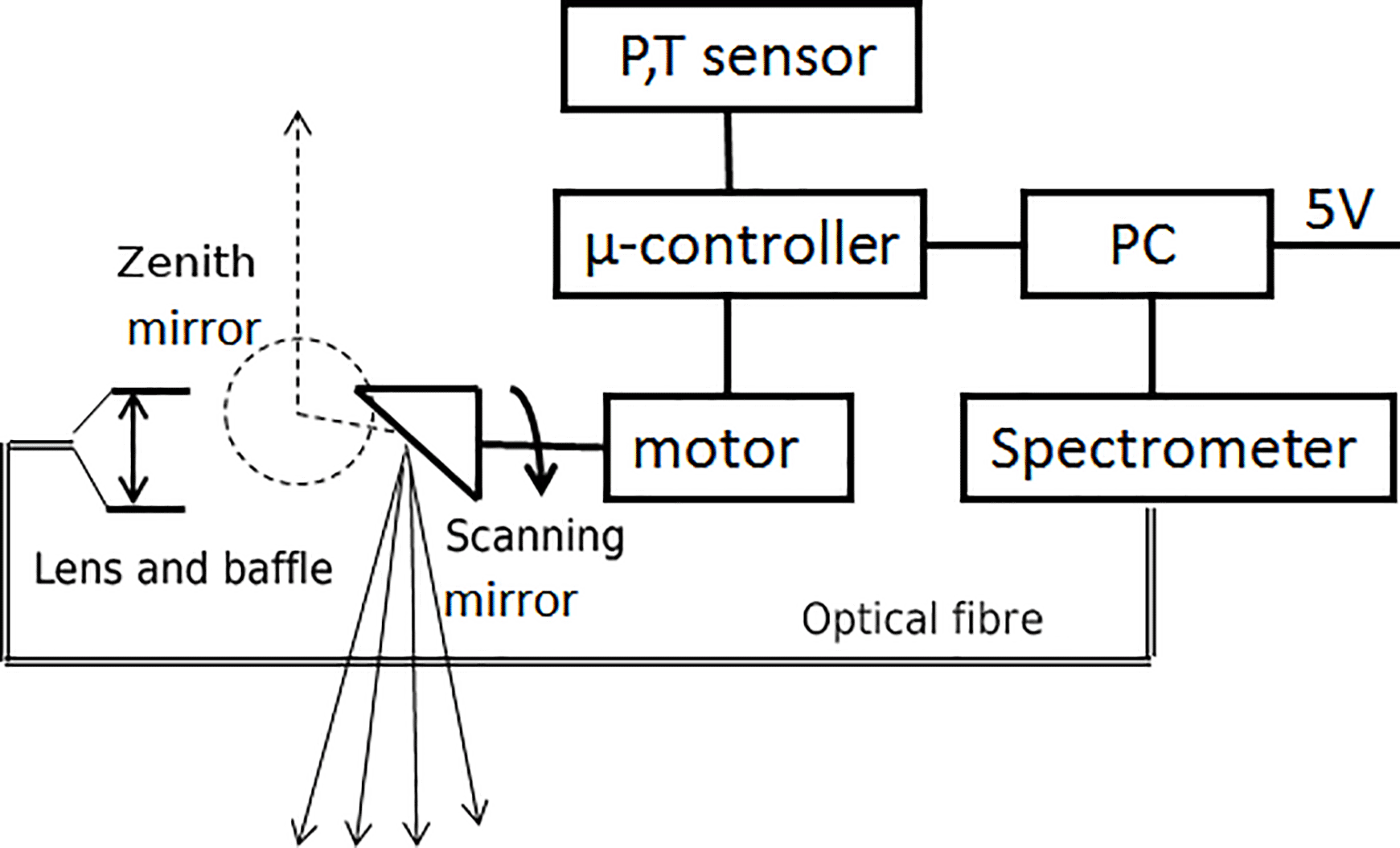
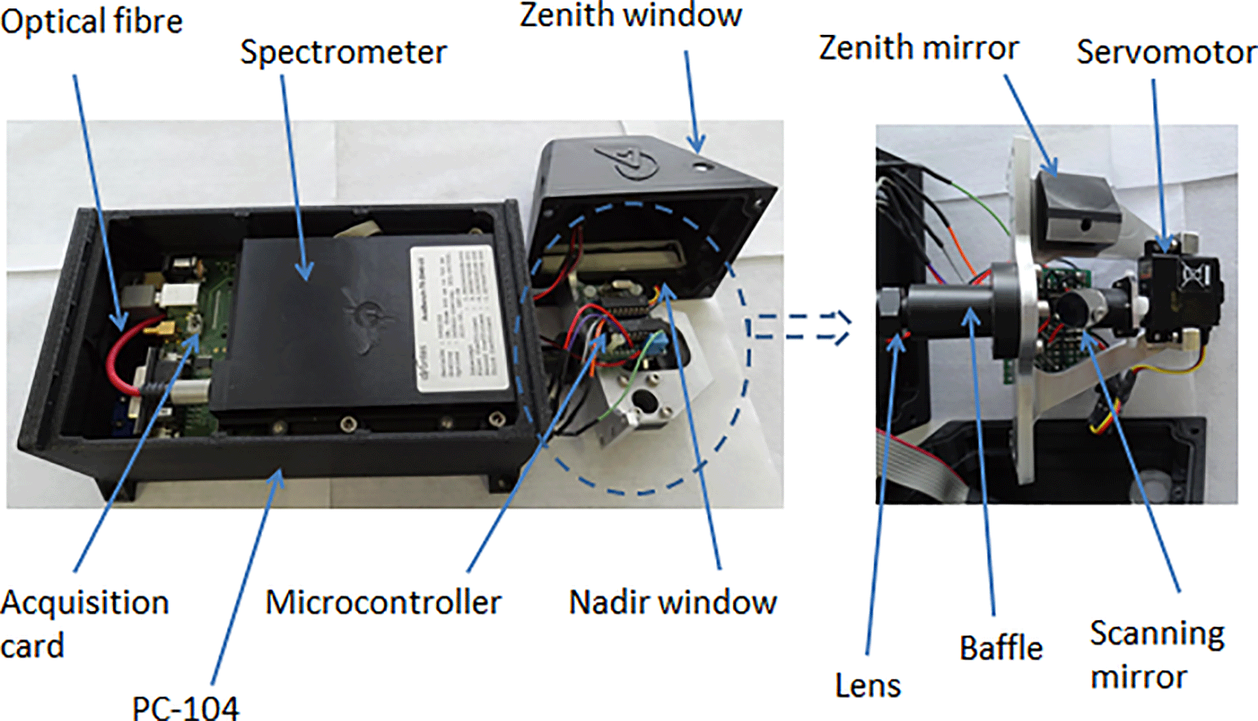
Figure 2The SWING instrument. Its dimensions are 27 cm × 12 cm × 8 cm and its weight is 920 g.
2.1 The SWING payload
The Small Whiskbroom Imager for atmospheric compositioN monitorinG (SWING) was developed at BIRA-IASB based on the experience gained with previous airborne DOAS instruments (Merlaud et al., 2011, 2012) and in the framework of a collaboration with the “Dunarea de Jos” University of Galati, Romania.
Figure 1 presents a schematic diagram of the SWING instrument, which is displayed with its open housing in Fig. 2. SWING is based on an Avantes AvaSpec-ULS2048 spectrometer, whose optical bench follows the Czerny–Turner design with a 75 mm focal length and a numerical aperture of 0.07. The entrance slit is 50 µm wide and the groove density of the grating is 600 L mm−1. The spectrometer covers the wavelength range 200–750 nm at a spectral resolution of 1.2 nm full width at half maximum (FWHM). The detector is a SONY ILX554B, which is an uncooled CCD linear array with 2048 pixels of 14 µm × 56 µm. SWING uses the standard Avantes AS-5216 microprocessor board with its 16 bit analogue-to-digital converter. This board reads a scan in 1.8 ms and is able to perform on-board signal processing such as averaging scans. In SWING, the spectrometer board is powered through USB by a PC-104 (Lippert CSR LX800), located under the spectrometer board. The PC-104 runs the acquisition software and stores the spectra. Both operations are performed on a 2 GB SSD integrated on the PC-104 to avoid the extra weight of an external disc.
SWING collects the light with a scanning mirror (elliptical Edmund Optics coated with enhanced aluminium, 12.7 mm × 17.96 mm). This mirror is mounted on the shaft of a HITEC HS-5056-MG servomotor which is controlled by an Arduino Micro. The latter also interfaces a pressure/temperature sensor (Bosch BMP180) and is linked to the PC-104 via USB. After the scanning mirror, light is collected by a fused silica collimating lens (an Avantes COL-UV/VIS, with a focal length of 8.7 mm and diameter of 6 mm) and through a 26 cm long optical fibre of 400 µm diameter. The mirror is able to scan at ±55∘ around the nadir direction. The instantaneous and angular fields of view (FOVs) are 2.6 and 110∘, respectively. It is also possible to record spectra in the zenith direction by rotating the scanning mirror at 90∘ relatively to nadir, pointing to a zenith mirror, which is adapted from an Avantes right-angle collimator (COL-90-UV/VIS).
Except the scanner support, which is made of aluminium, the structural parts of SWING and its housing are in plastic material (ABS). They were manufactured by 3-D printing to optimize their weight and shape. The optical windows are rectangular in nadir and circular in zenith. These windows are in Zeonex, a plastic material with a transmittance above 90 % between 350 and 1100 nm.
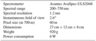
Table 1 summarizes the main characteristics of SWING. The weight, size, and power consumption of SWING are respectively 920 g, 27 cm × 12 cm × 8 cm, and 6 W. The whole system is powered by 5 V, which is supplied by a compact LiPo battery through an UBEC DC-DC converter. More technical details about the electronics circuits, miniaturization efforts, and first tests of SWING on an ultralight trike are presented in Merlaud (2013). The first test flights with SWING onboard the UAV were performed near Galati, Romania; these are presented in Merlaud et al. (2013).
2.2 The flying-wing UAV
Figure 3 shows the UAV which was used in this study. It was developed at the “Dunarea de Jos” University of Galati, in parallel with the development of SWING at BIRA-IASB. The aircraft is a flying-wing type with a 2.5 m wingspan. It is electrically propelled with LiPo batteries. The total mass of the system, including batteries, is 13 kg. The SWING payload is attached on the back of the wing and powered through its own LiPO battery. During flight, the GPS and attitude angles are recorded at 4 Hz on an SD card. The inertial sensor is an MPU 6050 from Invensense.
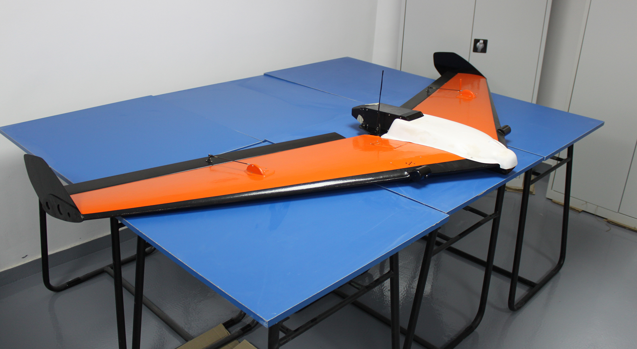
The UAV takes off with a catapult and lands on its belly. Airspeed is approximately 100 km h−1 and it has an autonomy of around 1 h depending on the flight pattern and wind conditions. The maximum flying altitude is 3 After take-off, the UAV can be piloted from the ground or operated in autopilot mode, following a pre-programmed flight pattern. Combining this with a real-time video link from a camera mounted on the UAV enables flying the aircraft beyond visual range. Note, however, that this was not possible during the AROMAT campaign due to a technical issue at the beginning of the campaign (see Sect. 3.2).
3.1 The AROMAT campaign
The Airborne ROmanian Measurements of Aerosols and Trace gases (AROMAT) campaign took place in Romania in September 2014. The AROMAT campaign was supported by the European Space Agency (ESA) in the framework of its Living Planet Programme. The primary objectives of the AROMAT campaign were (i) to test recently developed airborne observation systems dedicated to air quality satellite validation studies such as the AirMAP (Schönhardt et al., 2015), the KNMI NO2 sonde (Sluis et al., 2010), and SWING, and (ii) to prepare the validation programme of the future Atmospheric Sentinels, starting with Sentinel-5 Precursor.
The AROMAT campaign focused on two locations: the city of Bucharest (44.45∘ N, 26.1∘ E), the capital and largest city of Romania, and the large power plants of the Jiu Valley, in particular Turceni (44.67∘ N, 23.41∘ E; 116 ). Meier et al. (2017) present some of the work done during AROMAT in Bucharest. The SWING-UAV observations, which are the focus of this paper, were only performed in Turceni. Note that an overview presentation of AROMAT and its follow-up AROMAT-2 in August 2015 is the subject of a dedicated paper in preparation.
The coal-fired power station of Turceni is located in a rural area of the Jiu Valley, between the cities of Craiova and Targu Jiu and 210 km west of Bucharest. It is the largest power plant in Romania, producing 1600 MW of electricity. The power plant has four 280 m tall smokestacks. The Jiu Valley area and its power plants were chosen as geophysical targets of the AROMAT campaigns since emissions of NO2 and SO2 from this area are clearly visible from space, as was already observed two decades ago by Eisinger and Burrows (1998), and more recently by, for example, Krotkov et al. (2016).
3.2 The SWING-UAV flights in Turceni
We performed four SWING-UAV flights: one on 10 September and three on 11 September 2014. The UAV always took off from a flat grass field north of the power plant (44.68∘ N, 23.40∘ E; 116 ) and landed there as well. During the first three flights, we performed loops of 1.5 km diameter at around 700 around the take-off site. During these flights, SWING was scanning ±50∘ around nadir in steps of 4∘, and recording spectra with a total integration time of 400 ms (8×50 ms exposures). Zenith spectra of 2.5 s total integration time (500×5 ms) were acquired every 500 nadir spectra. Figure 4 shows the UAV track of the first flight (performed between 08:40 and 09:25 UTC) of 11 September 2014.
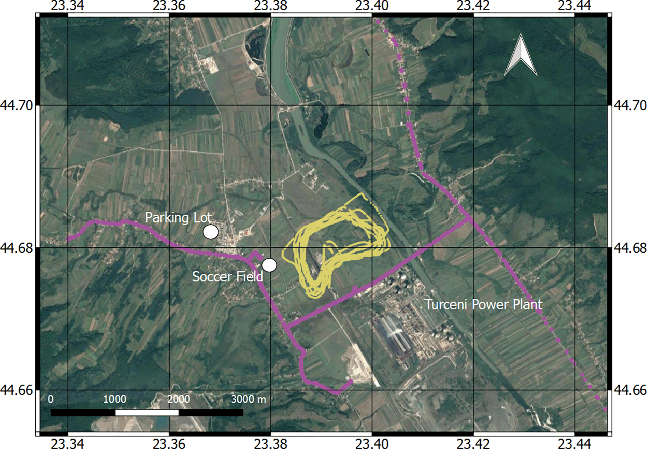
Figure 4The set-up in Turceni during the AROMAT campaign. The yellow loops indicate the UAV tracks during the first flight on 11 September 2014, while the pink line shows the roads simultaneously used by the mobile DOAS.
The fourth and last SWING-UAV flight (performed on 11 September 2014 between 14:58 and 15:10 UTC), was dedicated to vertical soundings. For this flight, the scanner was set in zenith position and SWING recorded spectra around zenith (given the varying plane attitude), with a total integration time of 1 s (with exposure times of 5 ms). The UAV made two successive ascents and descents, flying first to 700 , descending to 100 , then doing another ascent to 500 before landing. This flight pattern was intended to provide information on the absorbers vertical distribution.
Only the first and last flights of 11 September 2014 are analysed in this study. For the sake of clarity, we will hereafter refer to them as the mapping and sounding flights, respectively.
Note that a first flight was originally planned on 8 September 2014 but failed due to a pilot error at take-off. The UAV and the SWING payload were slightly damaged but could be quickly repaired on site. However, this led us to give up the use of the autopilot during the flights, for security reasons. Flying with the autopilot would have enabled us to cover a larger area and to adopt more efficient mapping patterns around the whole power plant. It would also have allowed for flying at higher altitude (1500 ), well above the emission plume of the power plant. Without autopilot, all the flights were performed in visual range with a permanent control of the UAV by the pilot on the ground. The flight patterns in this study are consequently not representative of the nominal capabilities of the SWING-UAV observation system.
3.3 Coincident measurements
The data analysis of the SWING-UAV experiments benefits from data collected with other instruments operated in Turceni during AROMAT, both in the air and from the ground.
Figure 4 describes the set-up of the AROMAT campaign in Turceni. As described in the previous section, the UAV was operated from the field to the north of the power plant. In the meantime, static ground-based measurements were performed at the Turceni soccer field (44.679∘ N, 23.378∘ E; 122 ). In particular, a scanning UV lidar (355 nm) was pointed toward the plume and used to determine the boundary layer height and estimate the aerosol extinction profile, a HORIBA APNA-370 was monitoring the volume mixing ratios of NOx at the surface and a weather station was recording the meteorological parameters (wind direction and speed, ground temperature and pressure, and relative humidity).
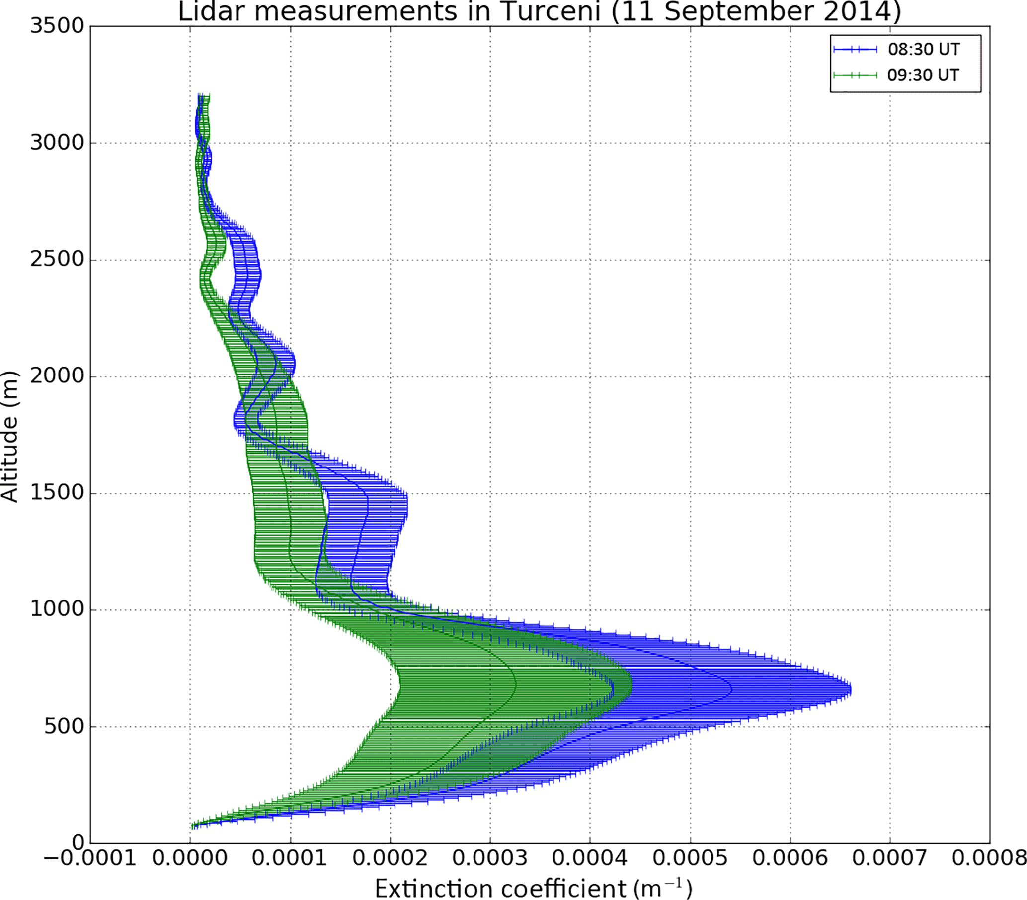

Figure 6Lower parts of two NO2 balloon-borne sonde measurements in Turceni on 11 September 2014. Panel (a) presents the profiles of relative humidity during the two soundings, (b) presents the potential temperature profiles, and (c) presents the NO2 profiles.
Figure 5 shows two extinction profiles retrieved from the lidar measurements around 09:00 UTC on 11 September 2014, when we performed the SWING-UAV NO2 experiment. The blind zone of the lidar above ground is 100 m thick. The two extinction profiles exhibit a rather similar shape, with a maximum extinction at 700 m, but the maximum decreases from to for 08:30 and 09:30 UTC, respectively.
Several KNMI NO2 sondes (Sluis et al., 2010) were launched on weather balloons on the days of the SWING-UAV observations. The balloons were launched from three different spots: the aforementioned UAV and soccer fields, and a parking lot in the village of Turceni (44.68∘ N, 23.37∘ E; 127 ; see Fig. 4). We tried several take-off sites for these balloons since it appeared difficult to cross the exhaust plume of the power plant with a wind-driven balloon.
Figure 6 presents the sonde measurements of relative humidity, potential temperature, and NO2 mixing ratio for the two balloon flights at 08:07 and 10:46 UTC on 11 September 2014. Both balloons were launched from the parking lot but, as can be seen from the NO2 profiles, the first one missed the main plume. The measurements at 10:46 UTC indicate that the main plume was then below 800 m, with a maximum detected volume mixing ratio (vmr) of 60 ppb close to this ceiling. The surface vmr is significantly lower (20 ppb), which can be understood from the emission height of the power plant stacks. An elevated NO2 layer is visible on both soundings: at 800 m at 08:07 UTC and at 1200 m at 10:46 UTC.
The sonde meteorological measurements enable to estimate the boundary layer height at the sounding times: around 700 m at 08:07 UTC and around 1100 m at 10:46 UTC. This second altitude is higher than the main plume, which indicates that the latter does not reach the top of the boundary layer. This is understandable since the NO2 field is sampled by the sonde very close to its source. The height and shape of the main NO2 plume appear in relative agreement with the lidar-retrieved extinction profile. Note that the elevated NO2 layer detected on both soundings appears close to the capping inversion, particularly visible in the morning balloon flight. The fact that it is also visible during the first sounding, which missed the main plume, and the mobile DOAS measurements (see below) indicates that this second plume has a larger horizontal extent than the main plume. This may indicate a remote origin, such as the power plants of Isalnita or Craiova, respectively located 40 and 50 km upwind of Turceni.
Finally, three DOAS instruments were operated during the SWING-UAV NO2 flight on 11 September 2014. The AirMAP (Schönhardt et al., 2015) instrument was mapping the plant exhaust plume from 3 km altitude on board the FUB Cessna, whereas a zenith-sky car-based DOAS system (Constantin et al., 2013) was operated along the roads marked in purple in Fig. 4. The measurements from these two DOAS instruments are compared with the SWING NO2 dataset in Sect. 5.1. The third DOAS instrument was a car-based system with two viewing directions (zenith and 30∘ above the horizon) (Merlaud, 2013). This instrument was installed on a car parked in the UAV field in front of the power plant during the SWING-UAV NO2 flight. Interestingly, this instrument missed the main plume during the UAV flight but did detect a small NO2 layer, with a vertical column density of 6×10¹⁵ molec cm−2. This value is consistent with the elevated layer of NO2 seen by both balloons. These static DOAS measurements are used (see Sect. 4.3) to estimate the column in the SWING reference spectrum.
Vandaele (1998)Thalman and Volkamer (2013)Thalman and Volkamer (2013)Rothman et al. (2010)Rothman et al. (2010)Bogumil et al. (2003)Bogumil et al. (2003)Chance and Spurr (1997)Chance and Spurr (1997)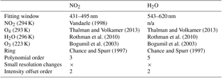

Figure 7Example of DOAS fits of NO2 and H2O in SWING spectra (a). The figure also shows O4 fits (b) and the fit residuals (c).
The data analysis starts with the DOAS analysis of the spectra, which extracts the molecular absorptions along the optical path of the measurements, namely the slant column densities (SCDs). These SCDs are then combined with the UAV position and attitude information. Regarding NO2, the georeferenced SCDs are converted to vertical column densities (VCDs) by modelling the light path. Regarding H2O, the SCDs recorded at different altitudes yield the volume mixing ratio of water vapour in between these altitudes.
4.1 Spectral analysis
DOAS analysis is a well-established technique (Platt and Stutz, 2008) to retrieve molecular absorptions in the UV–visible range. It is based on the fact that the absorption cross sections of certain molecules, such as NO2, O3, or H2O, vary much more rapidly with wavelength than Rayleigh and Mie scattering. In practice, the spectrum to analyse is divided by a reference spectrum to remove solar Fraunhofer structures and reduce instrumental effects. The components in the logarithm of this ratio (the measured optical depth) which vary slowly with the wavelength are filtered out by a low-order polynomial, while the remaining high-frequency structures are simultaneously fitted with high-pass-filtered laboratory cross sections. The DOAS analysis of a spectrum yields the integrated concentration of an absorber along the optical path of the measurement, with respect to the same quantity in the reference spectrum. This quantity is called the differential slant column density (DSCD).
Table 2 lists the DOAS analysis settings used in this study to retrieve NO2 and H2O DSCDs. We used the QDOAS software, which was developed at BIRA-IASB (Fayt et al., 2011; Danckaert et al., 2017), to analyse the spectra. In addition to interfering species (O3 and O4), we fitted the so-called Ring contribution (Grainger and Ring, 1962), which corresponds to the filling-in of the solar Fraunhofer lines caused by rotational Raman scattering on O2 and N2. For both species, we also fit an intensity offset and correct for small changes in spectral resolution during the flight. The latter is achieved by fitting a synthetic cross section corresponding to the derivative of the solar reference with respect to the slit function width (Beirle et al., 2017; Danckaert et al., 2017). Note that for the H2O fit, our DOAS settings are inspired by Wagner et al. (2013). As mentioned in Sect. 3.2, the scanner periodically took zenith spectra with a longer integration time (5 s). The reference spectra were chosen amongst these zenith measurements to minimize the absorber residual column, i.e. outside the NO2 plume and at the maximum altitude reached with the UAV.
Figure 7 shows typical DOAS fits for NO2 (left) and H2O (right) for spectra recorded from the UAV during the AROMAT campaign, together with the fitted O4 and the fit residuals. The ratio of the fitted DSCD to its uncertainty (an output of the DOAS analysis) yields an estimate of the signal-to-noise ratio of the DSCD measurements. It is around 18 for the NO2 DSCD inside the plume and 30 for the H2O DSCD. Note that the uncertainties also indicate the 1σ DSCD detection limit for the two species, i.e. and 1.4×10²¹ molec cm−2 for NO2 and H2O, respectively.
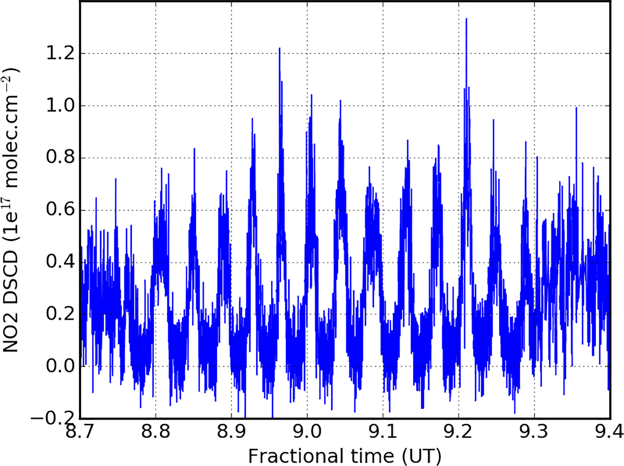
Figure 8 presents NO2 DSCD time series corresponding to the mapping flight on 11 September 2014. The UAV was performing loops at 700 , which are shown in Fig. 4. The NO2 DSCD times series indicates that the SWING line of sight crossed the plume at each loop, with a periodic pattern showing NO2 DSCD peaks between 0.06 and 1.3×10¹⁷ molec cm−2. This indicates that the UAV was flying at the border of the NO2 plume, as is further discussed in Sect. 5.1.
Figure 14a presents the H2O DSCD measurements corresponding to the sounding flight on 11 September 2014. As described in Sect. 3.2, the SWING scanner was set for zenith measurements during the entire flight. The two broad structures in the H2O DSCD correspond to the two successive ascents, the second one reaching a lower altitude. These H2O measurements are further discussed in Sect. 5.2.
Note that the DOAS retrieval of H2O is complicated by the non-linearity due to unresolved absorption lines. This leads to a saturation effect which becomes important at high SCDs, as investigated in Wagner et al. (2003). We have neglected this effect considering that we were only using zenith measurements in an area with relatively low H2O VCDs. The latter can be estimated from the balloon measurements to be around 9×10²² molec cm−2. The associated error could be around 5 %. In future SWING H2O measurements, this assumption should be checked especially if using off-zenith angles and when comparing with ancillary observations.
4.2 Georeferencing
As the SWING payload contains neither a GPS nor an attitude sensor, the SWING PC was synchronized to the GPS time before each flight. The georeferencing of the measurements was performed in post-processing using the UAV GPS and attitude data recorded on the SD card during the flight (see Sect. 2.2).
Figure 9 presents an excerpt of the time series of the attitude angles recorded by the UAV autopilot during the first flight on 11 September 2014. The excerpt corresponds to one of the UAV loops shown in Fig. 4. The roll lies between 30 and 60∘ and is mainly negative, indicating that the UAV keeps rotating in the same direction. The pitch angle lies between −12 and 30∘. Overall, the UAV attitude appears to vary a lot when compared to a manned aircraft flying at higher altitude. This is partly due to the turbulence in the boundary layer and would be reduced if flying in autopilot.
The attitude angles were used together with the UAV GPS measurements and the SWING scanner positions to georeference the SWING-UAV spectra and DSCDs using the geometric formulas given by Schönhardt et al. (2015).
4.3 Vertical columns of NO2
As described in Sect. 4.1, the DSCDs retrieved with the DOAS analysis depend not only on the absorber concentration but also (1) on the residual column in the reference spectrum and (2) on the light paths of the measurements. It is thus necessary to address both issues to get a more practical geophysical quantity, namely the vertical column density (VCD), i.e. the absorber concentrations integrated along the vertical path.
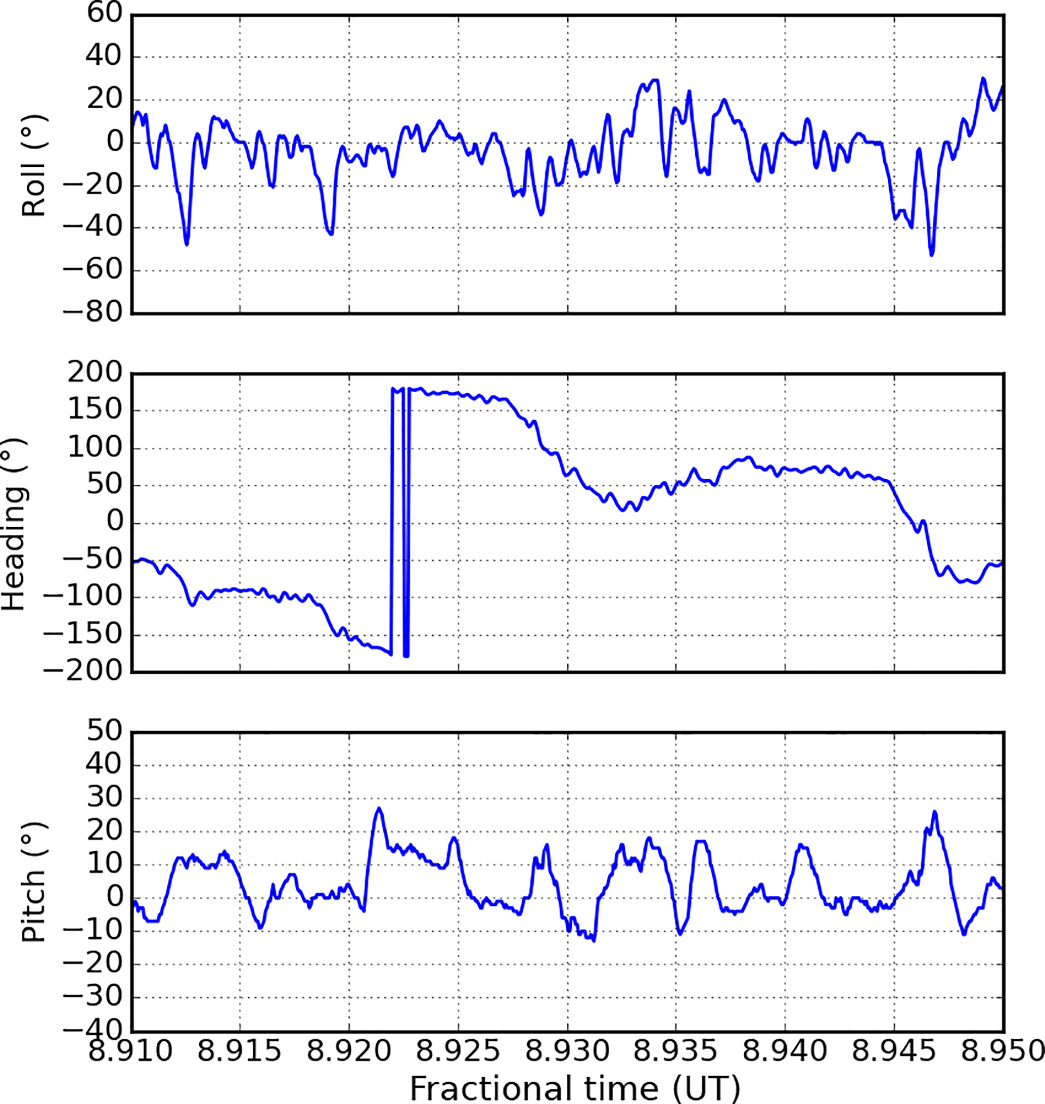
Figure 9Attitude angles measured by the UAV autopilot during one loop of the first flight on 11 September 2014.
The reference spectrum for NO2 was chosen among the SWING zenith spectra recorded at a high altitude and when the UAV was outside the main plume. The latter criterion could be checked with the coincident mobile DOAS measurements. However, as can be derived from the balloon-borne NO2 sonde measurements (see Fig. 6), a second layer of NO2 was present above the main plume, which covered a larger area. The absorption of this second layer is present in our reference spectrum and needs to be accounted for. The two sonde measurements lead to two different VCD values for this elevated NO2 layer, respectively 6.2×10¹⁵ molec cm−2 at 08:07 UTC, and 1.2×10¹⁶ molec cm−2 for the sonde at 10:46 UTC. None of these sondes was simultaneous with the SWING-UAV flight. However, the NO2 column of the elevated layer was measured during the UAV flight by the double-channel mobile DOAS, being around 6×10¹⁵ moles cm−2. Considering that the reference spectrum was recorded in zenith direction and assuming a geometric AMF of 1, this column value was used as the reference column (SCDref) to convert the DSCDs to SCDs according to
The light paths are accounted for in this study by estimating an air mass factor (AMF) for each spectrum. AMFs were calculated using the radiative transfer model UVspec/DISORT (Mayer and Kylling, 2005). The latter is based on the discrete ordinate method and deals with multiple scattering in the pseudo-spherical approximation. The ancillary measurements described in Sect. 3.3 were used as geophysical inputs: the profiles of NO2 and aerosol extinction were taken from the sonde (see Fig. 6) and lidar measurements (see Fig. 5), respectively. Meier et al. (2017) have developed a method to estimate the ground albedo from the uncalibrated radiances recorded by the AirMAP instrument. The ground albedo was not retrieved above Turceni, but we used the albedo value retrieved from AirMAP above a surface of similar type (grass) in the Bucharest flight of 8 September 2014, where the albedo was 0.02. The viewing angle varies for each spectrum due to the scanning and the variations in UAV attitude. This is accounted for by interpolating the AMFs on a look-up table built on a 10∘ grid of the viewing angle. The typical AMF for SWING-UAV nadir observations during AROMAT is 2.5. The VCD is then expressed as
The error on the retrieved VCD depends on the uncertainties on the elements of Eq. (2).
Note first that considering the short time span of the SWING-UAV flights (40 min), the stratospheric content of NO2 is assumed to be constant. Its contribution to the NO2 column thus cancels in the DSCD fit.
Regarding the reference NO2 column (SCDref), it was quantified by coincident mobile DOAS measurements. Its uncertainty is thus also neglected.
The uncertainties on the retrieved VCD originate then from two sources: the DSCD and the AMF.
The random error on the DSCD, σDSCD, is estimated during the DOAS analysis from the fit residuals, this is a standard output of the QDOAS software. We used this standard output as the uncertainty on our DSCD. Systematic uncertainties in the DSCD are mainly related to spectroscopy and are neglected in this study.
The error on the AMF depends on the errors on the radiative transfer model inputs with respect to the true state. Previous studies indicate that the two main uncertainty sources for nadir observations of the NO2 column are the ground albedo and the relative position of the NO2 and aerosol layer (Leitão et al., 2010; Meier et al., 2017; Tack et al., 2017). In our case, the lidar and sonde indicate that the NO2 and aerosols have a similar profile, as can be expected considering the large source in a rural area. On the other hand, as mentioned above, the ground albedo was estimated from albedo retrievals at another site three days before. The uncertainty on this parameter is therefore relatively large and we estimate it to 100 % of our value (i.e. ±0.02).
Figure 10 (upper panel) shows air mass factors calculated for flight altitudes of 0.8 and 3 km, in nadir geometry, and varying the albedo between 0.01 and 0.3. We took the aerosol profile and conditions of the AROMAT dataset as described above. The lower panel of Fig. 10 shows the box air mass factors for two albedos (0.02 and 0.2) for an altitude of 0.8 km (left) and 3 km (right), between the surface and 4 km altitude.
The AMF is larger for the low-altitude simulations (corresponding to SWING-UAV observations) when compared to higher altitude (AirMAP observations). This is understandable from the input NO2 profile and the box air mass factors: they indicate that, in both cases, the maximum sensitivity is right under the observation altitude. For the SWING-UAV observations, this means a maximum sensitivity inside the plume and thus a larger AMF when compared to AirMAP. Interestingly, the albedo dependency is also less pronounced for the low-altitude simulations. In both cases, reducing the albedo will increase the fraction of the collected photons which are back scattered in the atmosphere before hitting the ground, and thus decreases the AMF. The difference lies in the fact that for the high-altitude case, photons can be scattered above the plume, whereas for the low-altitude one, the scattering takes place within the plume anyway. In Fig. 10 (right lower panel), the box air mass factor remains above 2 between 1 and 2.5 km altitude for the low-albedo scenario, indicating a high sensitivity in this clean layers even for a low albedo.
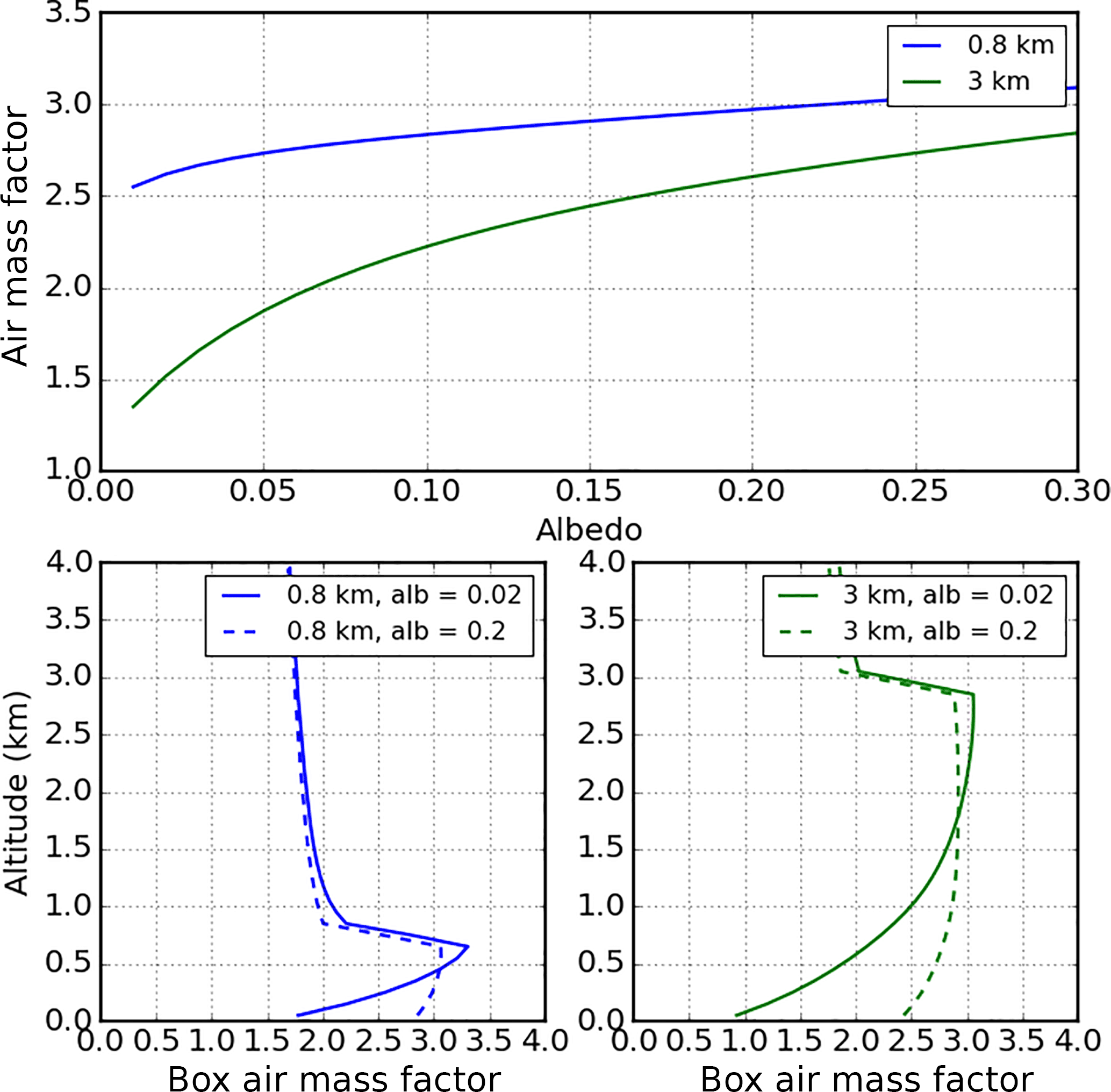
Figure 10Calculated nadir air mass factors in the AROMAT conditions, respectively from 800 m altitude and 3 km altitude.
Considering the uncertainty on the albedo discussed above (0.02), the AMF simulations were used to estimate an associated error (σAMF) of 0.2 on the AMF for the SWING retrievals. In practice, we consider a relative uncertainty of 10 % (ca. 0.25 in absolute values) on the AMF, to take into account other minor error sources.
The errors are then summed in quadrature to get the total error on the NO2 VCD:
These uncertainties are displayed as error bars in Fig. 13. They typically range between 2 and 4×10¹⁵ molec cm−2.
4.4 Volume mixing ratio of H2O
During the sounding flight (see Sect. 3.2), the scanner was fixed in zenith position. This flight was dedicated to sound the atmosphere vertically by performing two successive ascents and descents. Unfortunately, this flight missed most of the NO2 plume, but it appears possible to retrieve information on the water vapour abundance in the boundary layer.
Consider two zenith DSCD measurements of an absorber a recorded at different altitudes (A and B). Assuming that the light scattering is identical for the two measurements and that this scattering takes place above the highest of these two altitudes, the difference between the zenith DSCDs directly yields the partial VCD (VCDAB) between the two altitudes A and B:
This partial vertical column is by definition the concentration integrated vertically between A and B. Assuming air to be an ideal gas, this partial column can be expressed as
where Ca is the volume mixing ratio of the absorber a, p the air pressure, z the altitude, Na the Avogadro number, R the ideal gas constant, and T the air temperature.
Assuming a constant temperature and volume mixing ratio between A and B, and expressing the air pressure with the isothermal scale height (, where μ is the molar mass of air and g the acceleration of gravity), Eq. (5) leads to
where ΔPAB is the difference in pressure between the two altitudes A and B. It then follows the expression of Ca, the volume mixing ratio of a:
The uncertainty on Ca is obtained by propagating the errors on VCDAB. From Eq. (4) and assuming a similar uncertainty (σDSCD) on the DSCDs for A and B, the error on the volume mixing ratio is written as
Note that the above formula neglects the error on the measured pressure difference ΔPAB. From Eq. (7), we also assume that the molar mass of air (μ) is independent of the volume mixing ratio of the investigated absorber (Ca), which is wrong in principle. However, even for a large mixing ratio of water vapour in the boundary layer, the associated error is negligible when compared to the effect of the uncertainty on the DSCD. Note also that close to a large aerosol source like the Turceni power plant, the largest part of the uncertainty on Ca may originate from our very fist assumption, i.e. the assumed constant scattering conditions between the two altitudes. This could be wrong especially if the plane is below or inside the main exhaust plume for one of the two points.
The above equations are used hereafter (Sect. 5.2) to estimate the volume mixing ratio of water vapour in the boundary layer. This information could be used to estimate the optical properties of aerosols which depends on relative humidity, using for instance the OPAC model (Hess et al., 1998). Note also that the same technique may be used to retrieve information on the abundance and profile of other absorbers.
5.1 The horizontal distribution of NO2 around the power plant
Figure 11 presents two maps of the NO2 VCDs measured on 11 September 2014 around the Turceni power plant. The upper panel shows the AirMAP and mobile DOAS measurements, whereas the lower panel shows the SWING measurements. The plume extent appears clearly in the AirMAP data: originating from the power plant, the plume is pushed westwards by the wind. The width of the plume quickly increases to reach 2 km above the Turceni village, ca. 3 km downwind of the plant. The length of the plume is above 12 km, but it was not fully sampled by AirMAP. As expected, the horizontal gradients of the NO2 VCD field are steep, ranging from the background (around 2×10¹⁵ molec cm−2) to the plume (2×10¹⁶ molec cm−2) in a few hundred metres. The plume itself is not homogeneous but includes areas with NO2 VCDs above 2.5×10¹⁶ molec cm−2, not only close to the source but also along its entire observed length.
The SWING map on the lower panel of Fig. 11 covers a much smaller area than AirMAP, a circle with a diameter of approximately 3 km. Nevertheless, it shows the edge of the plume, which also enables observation of the sharp horizontal gradients of the NO2 field between the plume and the background. The absolute values of the NO2 VCDs retrieved from SWING appear similar to the ones retrieved from AirMAP. Note that the dashed white lines on the SWING map correspond to the edges of the plume as seen by AirMAP.
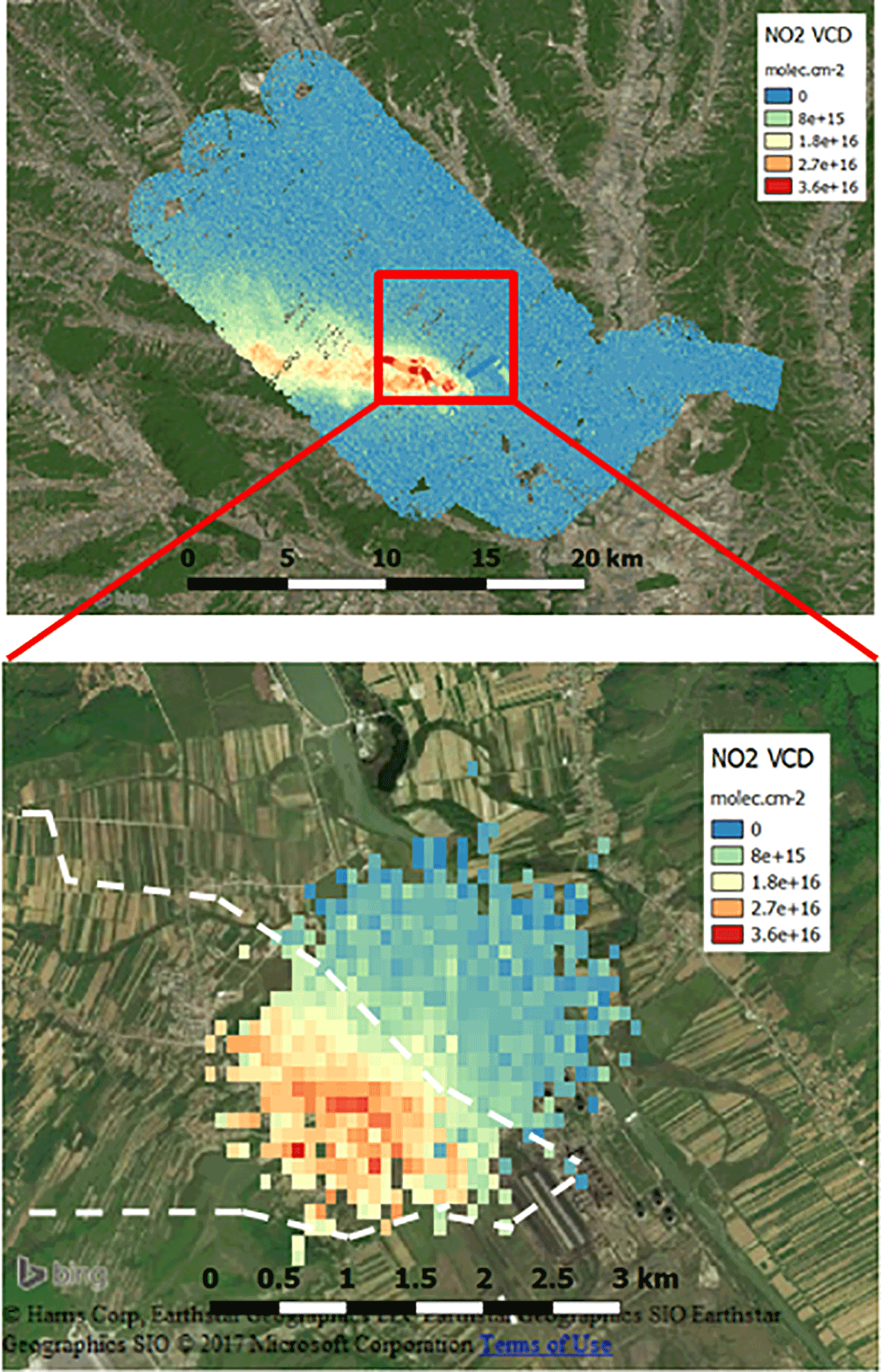
Figure 11SWING, AirMAP, and mobile DOAS measurements of NO2 in Turceni on 11 September 2014. The upper panel shows the AirMAP and mobile DOAS measurements (see text), while the lower panel shows the SWING measurements superimposed on the trace of the plume seen by AirMAP (dashed white line).

Figure 12 presents a scatter plot to compare quantitatively the AirMAP and SWING NO2 VCDs. The AirMAP measurements taken into account for this comparison were recorded in two adjacent flight lines, between 08:40 and 08:41 and between 08:48 and 08:50. These AirMAP data are almost perfectly time-coincident with the SWING-UAV measurements, which started at 08:40 and ended at 09:25. The AirMAP-SWING pairs of points were built in two steps. First, we applied a set of AMFs to the AirMAP slant columns. These AMFs are consistent with the ones used for SWING (see Sect. 4.3), adapting the altitudes and geometry to the AirMAP conditions but using the same ground albedo (0.02), NO2, and aerosol extinction profiles. Secondly, all AirMAP VCDs within 100 m of a SWING pixel were averaged to produce one averaged AirMAP point. AirMAP and SWING NO2 VCDs are up to 3.8 and 4.1×10¹⁶ molec cm−2, respectively. The Pearson correlation coefficient between the two dataset is 0.88, while the slope is 0.91, the AirMAP VCDs being slightly below the SWING ones. These higher values for the SWING VCDs with respect to AirMAP can also be seen in Fig. 13.
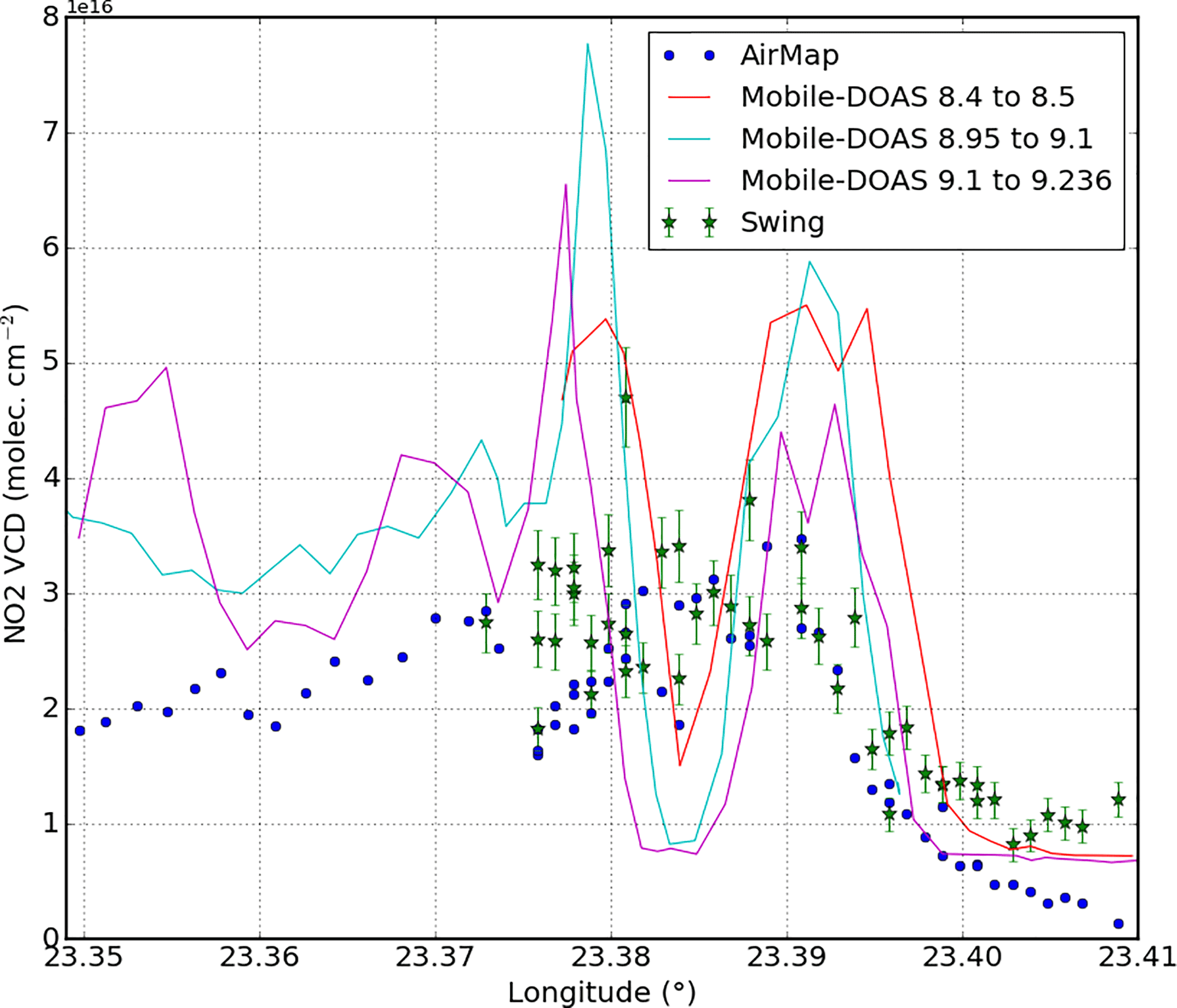
Figure 13SWING, AirMAP, and mobile DOAS NO2 VCD measurements along the mobile DOAS track on 11 September 2014.
We have also compared the two airborne DOAS products with time coincident car-based DOAS measurements. As mentioned in Sect. 3.3, the UGAL zenith-only mobile DOAS instrument was also operated during the SWING-UAV flight, along the road between the power plant and the village of Turceni.
Figure 13 presents the NO2 VCDs measurements by the three DOAS instruments along the road driven by the mobile DOAS (see Fig. 11) with respect to the longitude. The mobile DOAS did several drives, back and forth, along the road, but the main visible trends are stable. From east to west, the NO2 VCD increases as we enter the plume. This is visible for the three instruments and according to the mobile DOAS drives, the edge of the plume seems rather static at 23.395∘ E. However, the mobile DOAS data also show a dip in the NO2 VCDs at 23.382∘ E. This dip corresponds to the right angle turn close to the bottom of the red area in the upper panel of Fig. 11. It is close to the southern edge of the plume. Although this pattern appears to be reproducible in the three mobile DOAS drives of Fig. 13, it is not seen in the airborne data. Note that, both before and after the dip, the mobile DOAS VCDs are significantly higher (by approximately a factor of 2) than the airborne VCDs, but that this scaling factor is reduced in the western part, i.e. when the mobile DOAS was well inside the plume.
The differences observed between the two airborne DOAS systems may originate from the small time difference, which could be linked with variations in the power plant NO2 emissions. It could also be caused by errors on the radiative model inputs (in particular since a constant ground albedo is assumed). The comparison with the mobile DOAS also suggests another effect to take into account: the limitations of our 1-D radiative transfer model to take into account the complex 3-D geometry of the exhaust plume. Indeed, the airborne VCDs in Fig. 13 appear smoothed when compared to the mobile DOAS VCDs, which is understandable from the different light paths of the two types of measurements. At the time of the mapping flight, the solar zenith angle was close to 45∘. Assuming the NO2 plume to be 800 m thick, as the balloon flight indicates, leads to a horizontal smoothing of the same length for the airborne observations. Considering the sharp gradients of the NO2 field close to the power plant, this smoothing probably explains a major part of the difference between the aircraft and the mobile DOAS measurements. This motivates further investigation, both on practical intercomparison exercises and on theoretical work to estimate the optimal spatial resolution reachable with an airborne DOAS instrument, e.g. with 3-D radiative transfer models such as McArtim (Deutschmann et al., 2011).
5.2 Water vapour mixing ratio and relative humidity close to the ground
Figure 14 presents the time series of H2O DSCDs, pressure, and viewing zenith angle (VZA) as measured during the sounding flight on 11 September 2014 between 14:59 and 15:10 UTC. As described in Sect. 3.2, the SWING scanning mirror was fixed in upward position and the UAV performed two successive ascents, first to 700 m then to 500
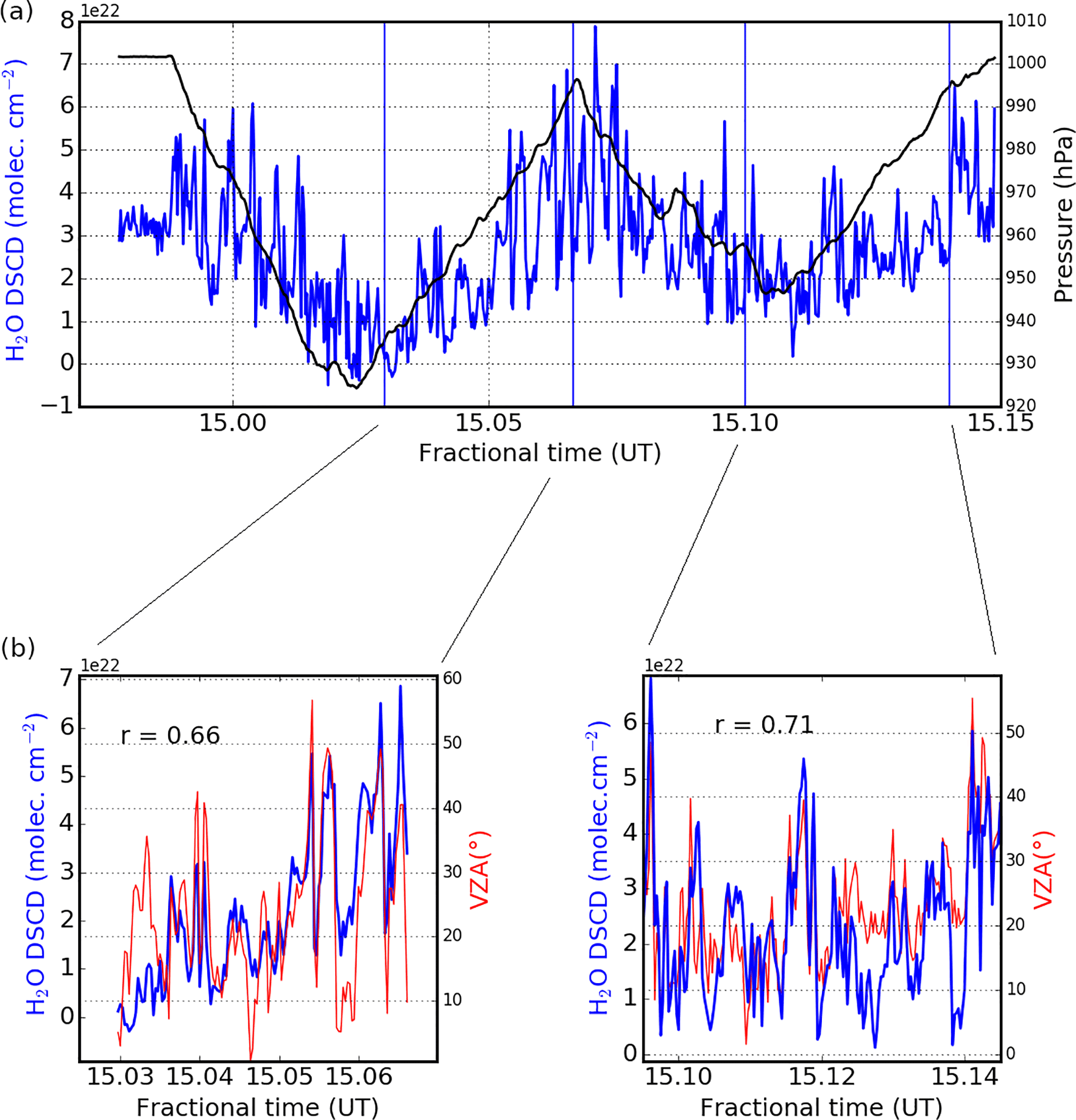
Figure 14Time series of H2O DSCDs and pressure (a), and of H2O DSCDs and VZA angles during the descents (b) on 11 September 2014.
The H2O DSCDs signal can be divided into two components, which are illustrated in the upper and lower panel of Fig. 14, respectively. First, there is a slow component visible in the upper panel, with two cycles during the flight. These changes are correlated with the variations in pressure, and thus in altitude. This slow part corresponds to the change of the remaining column of H2O above the UAV when its altitude changes. Secondly, the higher-frequency variations in the DSCD time series are related to the changes of the attitude of the UAV, and thus to changes in VZA. At first order, given an altitude and assuming a homogeneous H2O field, the slant column increases with VZA around its minimum value when the light path is vertical. This correlation is visible and quantified in the two time series extracted from the descents of the UAV in Fig. 14b.
We retrieved the volume mixing ratio of H2O as presented in Sect. 4.4. In practice, we selected two pairs of points during the flights where both the pitch and roll were under 2∘, and close to the ceiling and bottom of the flight, but above the surface to avoid the inhomogeneities close to the ground. These points are marked in the figure with blue vertical lines. Applying the formulas described in Sect. 4.4 to the two soundings leads to volume mixing ratios of 0.013 ± 0.002 and 0.012 ± 0.002 mol mol−1, respectively. Converting this value to a relative humidity yields, close to the surface, 41 and 39 %, respectively. There were no time coincident measurements of the relative humidity, but the balloon-borne measurements (see Fig. 6) show that it varied between 45 and 70 % in the boundary layer during the balloon flight at 10:46. These balloon observations are consistent with the surface measurements of the INOE weather station at the soccer field, which ran until 13:34, when the relative humidity was 38.8 %. As discussed in Sect. 4.1, these estimated humidities could be negatively biased by a few percent due to saturation of water vapour. They nevertheless appear realistic. It is worth noting that this experiment should be repeated with time coincident ancillary observations, but in other places. Indeed, the edge of a large exhaust plume of a power plant is clearly not optimal for the assumptions of homogeneity and simple scattering required for the retrieval.
The SWING instrument has been tested from a UAV during the AROMAT campaign in Romania, in September 2014. The SWING-UAV flights were performed in the vicinity of the Turceni power plant. Using the DOAS technique, the NO2 and H2O abundances were retrieved from the SWING spectra, and used to infer the horizontal distribution of NO2 VCDs and the volume mixing ratio of the water vapour in the boundary layer.
The retrieved SWING-UAV NO2 VCDs are up to molec cm−2 in the exhaust plume. They agree within 10 % with a time coincident airborne DOAS experiment, namely the AirMAP instrument, which was operated from a higher altitude. The SWING-UAV NO2 measurements were also compared with simultaneous mobile DOAS measurements from a car. The comparison is less good at the edge of the plume, which may be related to the effective spatial resolution achievable from a plane. Qualitatively, this resolution decreases with the solar zenith angle and the height of the NO2 layer. More theoretical work is required on this topic.
Regarding the H2O measurements, we retrieved a water vapour mixing ratio of 0.013 ± 0.002 mol mol−1 in the boundary layer. This finding could not be validated with time-coincident measurements, but it is consistent with observations performed a few hours before at the same location. To fully investigate the information content of this experiment, it should be repeated with ancillary observations in a cleaner area. Information on atmospheric water vapour could yield useful insights into aerosol optical properties.
The analysis scheme applied to get the H2O vmr from zenith spectra could be applied to NO2. This was not possible with the AROMAT dataset since the sounding flight missed the narrow NO2 plume. Performing this experiment would be easier in a smoother NO2 field such as in the exhaust plume of a large city.
The UAV was not operated in nominal mode during the AROMAT campaign, due to a technical problem. Overall, it appears an interesting and promising platform to study a local source in the countryside such as a remote power plant. Flying at low altitude increases the AMF and thus the sensitivity. The UAV is, however, limited in the areas it can cover, both because of the air traffic regulations and of the platform autonomy.
Because of the spectrometer limitations in the UV, the SWING-UAV observations of the first AROMAT campaign did not address SO2. This species is largely emitted by the coal-fired power plant of Turceni. To further investigate this, an updated version of the SWING instrument was built, with a better signal-to-noise ratio, especially in the UV. This new payload was installed on the FUB Cessna alongside the AirMAP instrument during the AROMAT-2 campaign in August 2015. These experiments will be described in a future study.
The data of the SWING observations can be obtained from the authors upon request.
The authors declare that they have no conflict of interest.
This article is part of the special issue “Airborne ROmanian Measurements of Aerosols and Trace gases (AROMAT)”. It is not associated with a conference.
The AROMAT activity was supported by ESA (contract 4000113511/15/NL/FF/gp)
and by the Belgian Space Policy (contract BR/121/PI/UAVReunion). Regarding
the AirMAP instrument, financial support through the University of Bremen
Institutional Strategy Measure M8 in the framework of the DFG Excellence
Initiative is gratefully acknowledged. We thank the people of Turceni and the
Air Traffic Control of Romania for their support and
cooperation.
Edited by: Jochen
Stutz
Reviewed by: two anonymous referees
Baidar, S., Oetjen, H., Coburn, S., Dix, B., Ortega, I., Sinreich, R., and Volkamer, R.: The CU Airborne MAX-DOAS instrument: vertical profiling of aerosol extinction and trace gases, Atmos. Meas. Tech., 6, 719–739, https://doi.org/10.5194/amt-6-719-2013, 2013. a
Bates, T. S., Quinn, P. K., Johnson, J. E., Corless, A., Brechtel, F. J., Stalin, S. E., Meinig, C., and Burkhart, J. F.: Measurements of atmospheric aerosol vertical distributions above Svalbard, Norway, using unmanned aerial systems (UAS), Atmos. Meas. Tech., 6, 2115–2120, https://doi.org/10.5194/amt-6-2115-2013, 2013. a
Beirle, S., Lampel, J., Lerot, C., Sihler, H., and Wagner, T.: Parameterizing the instrumental spectral response function and its changes by a super-Gaussian and its derivatives, Atmos. Meas. Tech., 10, 581–598, https://doi.org/10.5194/amt-10-581-2017, 2017. a
Berg, N., Mellqvist, J., Jalkanen, J.-P., and Balzani, J.: Ship emissions of SO2 and NO2: DOAS measurements from airborne platforms, Atmos. Meas. Tech., 5, 1085–1098, https://doi.org/10.5194/amt-5-1085-2012, 2012. a
Bogumil, K., Orphal, J., Homann, T., Voigt, S., Spietz, P., Fleischmann, O., Vogel, A., Hartmann, M., Kromminga, H., Bovensmann, H., Frerick, J., and Burrows, J.: Measurements of molecular absorption spectra with the SCIAMACHY pre-flight model: instrument characterization and reference data for atmospheric remote-sensing in the 230–2380 nm region, J. Photoch. Photobio. A., 157, 167–184, 2003. a, b
Bruns, M., Buehler, S. A., Burrows, J. P., Richter, A., Rozanov, A., Wang, P., Heue, K. P., Platt, U., Pundt, I., and Wagner, T.: NO2 Profile retrieval using airborne multi axis UV-visible skylight absorption measurements over central Europe, Atmos. Chem. Phys., 6, 3049–3058, https://doi.org/10.5194/acp-6-3049-2006, 2006. a
Cassano, J. J.: Observations of atmospheric boundary layer temperature profiles with a small unmanned aerial vehicle, Antarct. Sci., 26, 205–213, https://doi.org/10.1017/S0954102013000539, 2014. a
Chance, K. V. and Spurr, R. J. D.: Ring effect studies: Rayleigh scattering, including molecular parameters for rotational Raman scattering, and the Fraunhofer spectrum, Appl. Optics, 36, 5224–5230, https://doi.org/10.1364/AO.36.005224, 1997. a, b
Constantin, D., Merlaud, A., Van Roozendael, M., Voiculescu, M., Fayt, C., Hendrick, F., Pinardi, G., and Georgescu, L.: Measurements of tropospheric NO2 in Romania using a zenith-sky mobile DOAS system and comparisons with satellite observations, Sensors, 13, 3922–3940, https://doi.org/10.3390/s130303922, 2013. a
Constantin, D.-E., Merlaud, A., Voiculescu, M., Dragomir, C., Georgescu, L., Hendrick, F., Pinardi, G., and Van Roozendael, M.: Mobile DOAS observations of tropospheric NO2 using an UltraLight trike and flux calculation, Atmosphere-Basel, 8, 78, https://doi.org/10.3390/atmos8040078, 2017. a
Curry, J. A., Maslanik, J., Holland, G., and Pinto, J.: Applications of aerosondes in the Arctic, B. Am. Meteorol. Soc., 85, 1855–1861, https://doi.org/10.1175/BAMS-85-12-1855, 2004. a
Danckaert, T., Fayt, C., and Van Roozendael, M.: QDOAS, Software User Manual, Belgian Insitute for Space Aeronomy, Brussels, Belgium, 2017. a, b
Deutschmann, T., Beirle, S., Frieß, U., Grzegorski, M., Kern, C., Kritten, L., Platt, U., Prados-Román, C., Pukite, J., Wagner, T., Werner, B., and Pfeilsticker, K.: The Monte Carlo atmospheric radiative transfer model McArtim: introduction and validation of Jacobians and 3D features, J. Quant. Spectrosc. Ra., 112, 1119–1137, https://doi.org/10.1016/j.jqsrt.2010.12.009, 2011. a
Dix, B., Koenig, T. K., and Volkamer, R.: Parameterization retrieval of trace gas volume mixing ratios from Airborne MAX-DOAS, Atmos. Meas. Tech., 9, 5655–5675, https://doi.org/10.5194/amt-9-5655-2016, 2016. a
Eisinger, M. and Burrows, J. P.: Tropospheric sulfur dioxide observed by the ERS-2 GOME instrument, Geophys. Res. Lett., 25, 4177–4180, https://doi.org/10.1029/1998GL900128, 1998. a
Fayt, C., De Smedt, I., Letocart, V., Merlaud, A., Pinardi, G., and Van Roozendael, M.: QDOAS, Software User Manual, Belgian Insitute for Space Aeronomy, Brussels, Belgium, 2011. a
General, S., Pöhler, D., Sihler, H., Bobrowski, N., Frieß, U., Zielcke, J., Horbanski, M., Shepson, P. B., Stirm, B. H., Simpson, W. R., Weber, K., Fischer, C., and Platt, U.: The Heidelberg Airborne Imaging DOAS Instrument (HAIDI) – a novel imaging DOAS device for 2-D and 3-D imaging of trace gases and aerosols, Atmos. Meas. Tech., 7, 3459–3485, https://doi.org/10.5194/amt-7-3459-2014, 2014. a, b
Grainger, J. F. and Ring, J.: Anomalous Fraunhofer line profiles, Nature, 193, 762, https://doi.org/10.1038/193762a0, 1962. a
Hess, M., Koepke, P., and Schult, I.: Optical properties of aerosols and clouds: the software package OPAC, B. Am. Meteorol. Soc., 79, 831–844, 1998. a
Heue, K.-P., Wagner, T., Broccardo, S. P., Walter, D., Piketh, S. J., Ross, K. E., Beirle, S., and Platt, U.: Direct observation of two dimensional trace gas distributions with an airborne Imaging DOAS instrument, Atmos. Chem. Phys., 8, 6707–6717, https://doi.org/10.5194/acp-8-6707-2008, 2008. a
Holland, G. J., Webster, P. J., Curry, J. A., Tyrell, G., Gauntlett, D., Brett, G., Becker, J., Hoag, R., Vaglienti, W., Holland, G. J., Webster, P. J., Curry, J. A., Tyrell, G., Gauntlett, D., Brett, G., Becker, J., Hoag, R., and Vaglienti, W.: The Aerosonde Robotic Aircraft: a new paradigm for environmental observations, B. Am. Meteorol. Soc., 82, 889–901, https://doi.org/10.1175/1520-0477(2001)082<0889:TARAAN>2.3.CO;2, 2001. a
Houston, A. L., Argrow, B., Elston, J., Lahowetz, J., Frew, E. W., Kennedy, P. C., Houston, A. L., Argrow, B., Elston, J., Lahowetz, J., Frew, E. W., and Kennedy, P. C.: The collaborative Colorado–Nebraska unmanned aircraft system experiment, B. Am. Meteorol. Soc., 93, 39–54, https://doi.org/10.1175/2011BAMS3073.1, 2012. a
Illingworth, S., Allen, G., Percival, C., Hollingsworth, P., Gallagher, M., Ricketts, H., Hayes, H., Ładosz, P., Crawley, D., and Roberts, G.: Measurement of boundary layer ozone concentrations on-board a Skywalker unmanned aerial vehicle, Atmos. Sci. Lett., 15, 252–258, https://doi.org/10.1002/asl2.496, 2014. a
Kowalewski, M. G. and Janz, S. J.: Remote sensing capabilities of the Airborne Compact Atmospheric Mapper, Proc. SPIE 7452, Earth Observing Systems XIV, 74520Q, https://doi.org/10.1117/12.827035, 2009. a, b
Krotkov, N. A., McLinden, C. A., Li, C., Lamsal, L. N., Celarier, E. A., Marchenko, S. V., Swartz, W. H., Bucsela, E. J., Joiner, J., Duncan, B. N., Boersma, K. F., Veefkind, J. P., Levelt, P. F., Fioletov, V. E., Dickerson, R. R., He, H., Lu, Z., and Streets, D. G.: Aura OMI observations of regional SO2 and NO2 pollution changes from 2005 to 2015, Atmos. Chem. Phys., 16, 4605–4629, https://doi.org/10.5194/acp-16-4605-2016, 2016. a
Krotkov, N. A., Lamsal, L. N., Celarier, E. A., Swartz, W. H., Marchenko, S. V., Bucsela, E. J., Chan, K. L., Wenig, M., and Zara, M.: The version 3 OMI NO2 standard product, Atmos. Meas. Tech., 10, 3133–3149, https://doi.org/10.5194/amt-10-3133-2017, 2017. a
Lawrence, J. P., Anand, J. S., Vande Hey, J. D., White, J., Leigh, R. R., Monks, P. S., and Leigh, R. J.: High-resolution measurements from the airborne Atmospheric Nitrogen Dioxide Imager (ANDI), Atmos. Meas. Tech., 8, 4735–4754, https://doi.org/10.5194/amt-8-4735-2015, 2015. a
Leitão, J., Richter, A., Vrekoussis, M., Kokhanovsky, A., Zhang, Q. J., Beekmann, M., and Burrows, J. P.: On the improvement of NO2 satellite retrievals – aerosol impact on the airmass factors, Atmos. Meas. Tech., 3, 475–493, https://doi.org/10.5194/amt-3-475-2010, 2010. a
Lin, P.-H.: OBSERVATIONS: The first successful typhoon eyewall-penetration reconnaissance flight mission conducted by the unmanned aerial vehicle, aerosonde, B. Am. Meteorol. Soc., 87, 1481–1483, 2006. a
Mach, D., Blakeslee, R., Bailey, J., Farrell, W., Goldberg, R., Desch, M., and Houser, J.: Lightning optical pulse statistics from storm overflights during the Altus Cumulus Electrification Study, Atmos. Res., 76, 386–401, https://doi.org/10.1016/j.atmosres.2004.11.039, 2005. a
Martin, S., Bange, J., and Beyrich, F.: Meteorological profiling of the lower troposphere using the research UAV “M2AV Carolo”, Atmos. Meas. Tech., 4, 705–716, https://doi.org/10.5194/amt-4-705-2011, 2011. a
Mayer, B. and Kylling, A.: Technical note: The libRadtran software package for radiative transfer calculations – description and examples of use, Atmos. Chem. Phys., 5, 1855–1877, https://doi.org/10.5194/acp-5-1855-2005, 2005. a
Mayer, S., Sandvik, A., Jonassen, M. O., and Reuder, J.: Atmospheric profiling with the UAS SUMO: a new perspective for the evaluation of fine-scale atmospheric models, Meteorol. Atmos. Phys., 116, 15–26, https://doi.org/10.1007/s00703-010-0063-2, 2012. a
Meier, A. C., Schönhardt, A., Bösch, T., Richter, A., Seyler, A., Ruhtz, T., Constantin, D.-E., Shaiganfar, R., Wagner, T., Merlaud, A., Van Roozendael, M., Belegante, L., Nicolae, D., Georgescu, L., and Burrows, J. P.: High-resolution airborne imaging DOAS measurements of NO2 above Bucharest during AROMAT, Atmos. Meas. Tech., 10, 1831–1857, https://doi.org/10.5194/amt-10-1831-2017, 2017. a, b, c, d
Melamed, M. L., Solomon, S., Daniel, J. S., Langford, A. O., Portmann, R. W., Ryerson, T. B., Nicks, Jr., D. K., McKeen, S. A., McKeen, S. A., Parrish, D. D., Roberts, J. M., Sueper, D. T., Trainer, M., Williams, J., and Fehsenfeld, F. C.: Measuring reactive nitrogen emissions from point sources using visible spectroscopy from aircraft, J. Environ. Monitor., 5, 29–34, https://doi.org/10.1039/b204220g, 2003. a
Merlaud, A.: Development and Use of Compact Instruments for Tropospheric Investigations Based on Optical Spectroscopy from Mobile Platforms, Presses univ. de Louvain, 2013. a, b
Merlaud, A., Van Roozendael, M., Theys, N., Fayt, C., Hermans, C., Quennehen, B., Schwarzenboeck, A., Ancellet, G., Pommier, M., Pelon, J., Burkhart, JMerlaud, A., Van Roozendael, M., Theys, N., Fayt, C., Hermans, C., Quennehen, B., Schwarzenboeck, A., Ancellet, G., Pommier, M., Pelon, J., Burkhart, J., Stohl, A., and De Mazière, M.: Airborne DOAS measurements in Arctic: vertical distributions of aerosol extinction coefficient and NO2 concentration, Atmos. Chem. Phys., 11, 9219–9236, https://doi.org/10.5194/acp-11-9219-2011, 2011. a, b
Merlaud, A., Van Roozendael, M., van Gent, J., Fayt, C., Maes, J., Toledo-Fuentes, X., Ronveaux, O., and De Mazière, M.: DOAS measurements of NO2 from an ultralight aircraft during the Earth Challenge expedition, Atmos. Meas. Tech., 5, 2057–2068, https://doi.org/10.5194/amt-5-2057-2012, 2012. a
Merlaud, A., Constantin, D. E., Mingireanu, F., Mocanu, I., Fayt, C., Maes, J., Murariu, G., Voiculescu, M., Georgescu, L., and Van Roozendael, M.: Small whiskbroom imager for atmospheric compositioN monitoring (SWING) from an Unmanned Aerial Vehicle (UAV), ESA Sp. Publ., 721, 233–239, 2013. a
Nowlan, C. R., Liu, X., Leitch, J. W., Chance, K., González Abad, G., Liu, C., Zoogman, P., Cole, J., Delker, T., Good, W., Murcray, F., Ruppert, L., Soo, D., Follette-Cook, M. B., Janz, S. J., Kowalewski, M. G., Loughner, C. P., Pickering, K. E., Herman, J. R., Beaver, M. R., Long, R. W., Szykman, J. J., Judd, L. M., Kelley, P., Luke, W. T., Ren, X., and Al-Saadi, J. A.: Nitrogen dioxide observations from the Geostationary Trace gas and Aerosol Sensor Optimization (GeoTASO) airborne instrument: Retrieval algorithm and measurements during DISCOVER-AQ Texas 2013, Atmos. Meas. Tech., 9, 2647–2668, https://doi.org/10.5194/amt-9-2647-2016, 2016. a
Pfeilsticker, K. and Platt, U.: Airborne measurements during the Arctic Stratospheric Experiment: observation of O3 and NO2, Geophys. Res. Lett., 21, 1375–1378, https://doi.org/10.1029/93GL01870, 1994. a
Platt, U. and Stutz, J.: Differential Optical Absorption Spectroscopy: Principles and Applications, Physics of Earth and Space Environments, Springer, Berlin, 2008. a, b
Popp, C., Brunner, D., Damm, A., Van Roozendael, M., Fayt, C., and Buchmann, B.: High-resolution NO2 remote sensing from the Airborne Prism EXperiment (APEX) imaging spectrometer, Atmos. Meas. Tech., 5, 2211–2225, https://doi.org/10.5194/amt-5-2211-2012, 2012. a
Prados-Roman, C., Butz, A., Deutschmann, T., Dorf, M., Kritten, L., Minikin, A., Platt, U., Schlager, H., Sihler, H., Theys, N., Van Roozendael, M., Wagner, T., and Pfeilsticker, K.: Airborne DOAS limb measurements of tropospheric trace gas profiles: case studies on the profile retrieval of O4 and BrO, Atmos. Meas. Tech., 4, 1241–1260, https://doi.org/10.5194/amt-4-1241-2011, 2011. a
Reuder, J., Brisset, P., Jonassen, M., Müller, M., and Mayer, S.: The Small Unmanned Meteorological Observer SUMO: a new tool for atmospheric boundary layer research, Meteorol. Z., 18, 141–147, https://doi.org/10.1127/0941-2948/2009/0363, 2009. a
Rothman, L., Gordon, I., Barber, R., Dothe, H., Gamache, R., Goldman, A., Perevalov, V., Tashkun, S., and Tennyson, J.: HITEMP, the high-temperature molecular spectroscopic database, J. Quant. Spectrosc. Ra., 111, 2139–2150, https://doi.org/10.1016/j.jqsrt.2010.05.001, 2010. a, b
Schönhardt, A., Altube, P., Gerilowski, K., Krautwurst, S., Hartmann, J., Meier, A. C., Richter, A., and Burrows, J. P.: A wide field-of-view imaging DOAS instrument for two-dimensional trace gas mapping from aircraft, Atmos. Meas. Tech., 8, 5113–5131, https://doi.org/10.5194/amt-8-5113-2015, 2015. a, b, c, d
Sluis, W. W., Allaart, M. A. F., Piters, A. J. M., and Gast, L. F. L.: The development of a nitrogen dioxide sonde, Atmos. Meas. Tech., 3, 1753–1762, https://doi.org/10.5194/amt-3-1753-2010, 2010. a, b
Spiess, T., Bange, J., Buschmann, M., and Vörsmann, P.: First application of the meteorological Mini-UAV 'M2AV', Meteorol. Z., 16, 159–169, https://doi.org/10.1127/0941-2948/2007/0195, 2007. a
Stephens, G. L., Miller, S. D., Benedetti, A., McCoy, R. B., McCoy, R. F., Ellingson, R. G., Vitko, J., Bolton, W., Tooman, T. P., Valero, F. P. J., Minnis, P., Pilewskie, P., Phipps, G. S., Sekelsky, S., Carswell, J. R., Lederbuhr, A., and Bambha, R.: The Department of Energy's Atmospheric Radiation Measurement (ARM) Unmanned Aerospace Vehicle (UAV) program, B. Am. Meteorol. Soc., 81, 2915–2938, https://doi.org/10.1175/1520-0477(2000)081<2915:TDOESA>2.3.CO;2, 2000. a
Stutz, J., Werner, B., Spolaor, M., Scalone, L., Festa, J., Tsai, C., Cheung, R., Colosimo, S. F., Tricoli, U., Raecke, R., Hossaini, R., Chipperfield, M. P., Feng, W., Gao, R.-S., Hintsa, E. J., Elkins, J. W., Moore, F. L., Daube, B., Pittman, J., Wofsy, S., and Pfeilsticker, K.: A new Differential Optical Absorption Spectroscopy instrument to study atmospheric chemistry from a high-altitude unmanned aircraft, Atmos. Meas. Tech., 10, 1017–1042, https://doi.org/10.5194/amt-10-1017-2017, 2017. a
Tack, F., Merlaud, A., Iordache, M.-D., Danckaert, T., Yu, H., Fayt, C., Meuleman, K., Deutsch, F., Fierens, F., and Van Roozendael, M.: High-resolution mapping of the NO2 spatial distribution over Belgian urban areas based on airborne APEX remote sensing, Atmos. Meas. Tech., 10, 1665–1688, https://doi.org/10.5194/amt-10-1665-2017, 2017. a, b
Thalman, R. and Volkamer, R.: Temperature dependent absorption cross-sections of O2–O2 collision pairs between 340 and 630 nm and at atmospherically relevant pressure, Phys. Chem. Chem. Phys., 15, 15371, https://doi.org/10.1039/c3cp50968k, 2013. a, b
Vandaele, A.: Measurements of the NO2 absorption cross-section from 42 000 cm−1 to 10 000 cm−1 (238–1000 nm) at 220 K and 294 K, J. Quant. Spectrosc. Ra., 59, 171–184, https://doi.org/10.1016/S0022-4073(97)00168-4, 1998. a
van den Kroonenberg, A., Martin, T., Buschmann, M., Bange, J., and Vörsmann, P.: Measuring the wind vector using the autonomous mini aerial vehicle M2 AV, J. Atmos. Ocean. Tech., 25, 1969–1982, https://doi.org/10.1175/2008JTECHA1114.1, 2008. a
Wagner, T., Heland, J., Zöger, M., and Platt, U.: A fast H2O total column density product from GOME – Validation with in-situ aircraft measurements, Atmos. Chem. Phys., 3, 651–663, https://doi.org/10.5194/acp-3-651-2003, 2003. a
Wagner, T., Andreae, M. O., Beirle, S., Dörner, S., Mies, K., and Shaiganfar, R.: MAX-DOAS observations of the total atmospheric water vapour column and comparison with independent observations, Atmos. Meas. Tech., 6, 131–149, https://doi.org/10.5194/amt-6-131-2013, 2013. a
Wahner, A., Jakoubek, R. O., Mount, G. H., Ravishankara, A. R., and Schmeltekopf, A. L.: Remote sensing observations of daytime column NO2 during the Airborne Antarctic Ozone Experiment, August 22 to October 2, 1987, J. Geophys. Res., 94, 16619, https://doi.org/10.1029/JD094iD14p16619, 1989. a
Wang, P., Richter, A., Bruns, M., Rozanov, V. V., Burrows, J. P., Heue, K.-P., Wagner, T., Pundt, I., and Platt, U.: Measurements of tropospheric NO2 with an airborne multi-axis DOAS instrument, Atmos. Chem. Phys., 5, 337–343, https://doi.org/10.5194/acp-5-337-2005, 2005. a
Watai, T., Machida, T., Ishizaki, N., and Inoue, G.: A lightweight observation system for atmospheric carbon dioxide concentration using a small unmanned aerial vehicle, J. Atmos. Ocean. Tech., 23, 700–710, https://doi.org/10.1175/JTECH1866.1, 2006. a
Watts, A. C., Ambrosia, V. G., and Hinkley, E. A.: Unmanned aircraft systems in remote sensing and scientific research: classification and considerations of use, Remote Sens.-Basel, 4, 1671–1692, https://doi.org/10.3390/rs4061671, 2012. a