the Creative Commons Attribution 4.0 License.
the Creative Commons Attribution 4.0 License.
 | 12 Oct 2018
Cloud fraction determined by thermal infrared and visible all-sky cameras
Julian Gröbner
Niklaus Kämpfer
The thermal infrared cloud camera (IRCCAM) is a prototype instrument that determines cloud fraction continuously during daytime and night-time using measurements of the absolute thermal sky radiance distributions in the 8–14 µm wavelength range in conjunction with clear-sky radiative transfer modelling. Over a time period of 2 years, the fractional cloud coverage obtained by the IRCCAM is compared with two commercial cameras (Mobotix Q24M and Schreder VIS-J1006) sensitive in the visible spectrum, as well as with the automated partial cloud amount detection algorithm (APCADA) using pyrgeometer data. Over the 2-year period, the cloud fractions determined by the IRCCAM and the visible all-sky cameras are consistent to within 2 oktas (0.25 cloud fraction) for 90 % of the data set during the day, while for day- and night-time data the comparison with the APCADA algorithm yields an agreement of 80 %. These results are independent of cloud types with the exception of thin cirrus clouds, which are not detected as consistently by the current cloud algorithm of the IRCCAM. The measured absolute sky radiance distributions also provide the potential for future applications by being combined with ancillary meteorological data from radiosondes and ceilometers.


Clouds affect the surface radiation budget and thus the climate system on a local as well as on a global scale. Clouds have an influence on solar and on terrestrial radiation by absorbing, scattering and emitting radiation. The Intergovernmental Panel on Climate Change (IPCC) states that clouds in general, and aerosol–cloud interactions in particular, generate considerable uncertainty in climate predictions and climate models (IPCC, 2013). Having information about cloud fraction on a local scale is of importance in different fields: for solar power production due to the fact that clouds cause large variability in the energy production (Mateos et al., 2014; Parida et al., 2011; Tzoumanikas et al., 2016), for aviation and weather forecast or microclimatological studies.
The most common practice worldwide used to determine cloud coverage, cloud base height (CBH) and cloud type from the ground are human observations (CIMO, 2014). These long-term series of cloud data allow climate studies to be conducted (Chernokulsky et al., 2017). Cloud detection by human observers is carried out several times per day over a long time period without the risk of a larger data gap due to the technical failure of an instrument. However, even with a reference standard defined by the World Meteorological Organisation (WMO), for human observers, the cloud determination is not objective, e.g. due to varying degrees of experience (Boers et al., 2010). Other disadvantages of human cloud observations are that the temporal resolution is coarse and, due to visibility issues, night-time determinations are difficult. Since clouds are highly variable in space and time, measurements at high spatial and temporal resolution with small uncertainties are needed (WMO, 2012). Recent research has therefore been conducted to find an automated cloud detection instrument (or a combination of instruments) to replace human observers (Boers et al., 2010; Huertas-Tato et al., 2017; Smith et al., 2017; Tapakis and Charalambides, 2013).
An alternative to detecting clouds from the ground by human observation is to detect them from space. With a temporal resolution of 5 to 15 min, Meteosat Second Generation (MSG) geostationary satellites are able to detect cloud coverage with a higher time resolution than is accomplished by human observers (Ricciardelli et al., 2010; Werkmeister et al., 2015). The geostationary satellite Himawari-8 (Da, 2015) even delivers cloud information with a temporal resolution of 2.5 to 10 min and a spatial resolution of 0.5 to 2 km. However, these geostationary satellites cover only a certain region of the globe. Circumpolar satellites (i.e. the MODIS satellites Terra and Aqua, Ackerman et al., 2008; Baum and Platnick, 2006) determine cloud fraction globally, but for a specific region only four times a day. Satellites cover a larger area than ground-based instruments and are also able to deliver cloud information from regions where few ground-based instruments are available (e.g. in Arctic regions Heymsfield et al., 2017 or over oceans). However, due to the limited resolution of satellites, small clouds can be overlooked (Ricciardelli et al., 2010). Another challenge with satellite data is the ability to distinguish thin clouds from land (Ackerman et al., 2008; Dybbroe et al., 2005). Furthermore, satellites collect information mainly from the highest cloud layer rather than the lower cloud layer, closer to the Earth's surface. Satellite data are validated and thus supported by ground-based cloud data. Different studies focusing on the comparison of the determined cloud fraction from ground and from space were presented, e.g. by Fontana et al. (2013), Wacker et al. (2015), Calbó et al. (2016), Kotarba (2017).
In general, three automatic ground-based cloud cover measurement techniques are distinguished: radiometers, active column instruments and hemispherical sky cameras. Radiometers measure the incident radiation in different wavelength ranges. Depending on the wavelength range, the presence of clouds alters the radiation measured at ground level (Calbó et al., 2001; Mateos Villán et al., 2010). Calbó et al. (2001) and Dürr and Philipona (2004) both present different methodologies to determine cloud conditions from broadband radiometers. Other groups describe methodologies using instruments with a smaller spectral range. Such instruments are, for example, the infrared pyrometer CIR-7 (Nephelo) (Tapakis and Charalambides, 2013) or NubiScope (Boers et al., 2010; Brede et al., 2017; Feister et al., 2010), which both measure in the 8–14 µm wavelength range of the spectrum. In order to retrieve cloud information, Nephelo consists of seven radiometers which scan the whole of the upper hemisphere. The NubiScope consists of one radiometer only, which also scans the whole of the upper hemisphere. A scan takes several minutes, which is a limitation on the retrieval of cloud fraction information when, for example, fast-moving clouds occur (Berger et al., 2005). In general, these instruments give information about cloud fraction for three different levels, cloud types and CBH (Wauben, 2006). Brocard et al. (2011) presents a method using data from the tropospheric water vapour radiometer (TROWARA) to determine cirrus clouds from the measured fluctuations in the sky infrared brightness temperature.
The second group, the column cloud detection instruments, send laser pulses to the atmosphere and measure the backscattered photons. The photons are scattered back by hydrometeors in clouds and, depending on the time and the amount of backscattered photons measured, the cloud base height can be determined. However, the laser pulse is not only scattered back by cloud hydrometeors, but also by aerosols (Liu et al., 2015). Examples of active remote sensing instruments are cloud radar (Feister et al., 2010; Illingworth et al., 2007; Kato et al., 2001), lidar (Campbell et al., 2002; Zhao et al., 2014) and ceilometers (Martucci et al., 2010). Due to the narrow beam, a disadvantage of these measurement techniques is the lack of instantaneous cloud information of the whole of the upper hemisphere. Boers et al. (2010) showed that, with smaller integration times, the instruments tend to give okta values of 0 and 8 rather than the intermediate cloud fractions of 1 to 7 oktas.
The third group of ground-based cloud detection instruments comprises the hemispherical sky cameras, which often have a 180∘ view of the upper hemisphere. The most common all-sky camera is the commercially available Total Sky Imager (TSI) (Long et al., 2006). Another pioneering hemispherical cloud detection instrument is the Whole Sky Imager (WSI) (Shields et al., 2013). Whereas the TSI is sensitive in the visible spectrum, the WSI acquires information in seven different spectral ranges in the visible and in the near infrared regions. A special version of the WSI also allows for night-time measurements (Feister and Shields, 2005). Other cloud research has been undertaken with low-cost commercial cameras sensitive in the visible spectrum of the wavelength range (Calbó and Sabburg, 2008; Cazorla et al., 2008; Kazantzidis et al., 2012; Kuhn et al., 2017; Wacker et al., 2015). All of these hemispherical sky cameras operate well during the daytime but give often limited information during night-time. Thus, there is increasing interest in the development of cloud cameras sensitive in the thermal infrared region of the spectrum. Ground-based thermal infrared all-sky cameras have the advantage of potentially delivering continuous information about cloud coverage, cloud base height and cloud type during daytime and night-time, which in turn is of interest in various fields.
The Infrared Cloud Imager (ICI) is a ground-based sky camera sensitive in the 8–14 µm wavelength range and with a resolution of 320×240 pixels (Shaw et al., 2005; Smith and Toumi, 2008; Thurairajah and Shaw, 2005). Another instrument, the Solmirus All Sky Infrared Visible Analyzer (ASIVA) consists of two cameras, one measuring in the visible and the other one in the 8–13 µm wavelength range (Klebe et al., 2014). The whole-sky infrared cloud measuring system (WSIRCMS) is an all-sky cloud camera sensitive in the 8–14 µm wavelength range (Liu et al., 2013). The WSIRCMS consists of nine cameras measuring at the zenith and at eight surrounding positions. With a time resolution of 15 min, information about cloud cover, CBH and cloud type are determined. This instrument has an accuracy of ±0.3 oktas compared to visual observations (Liu et al., 2013). Redman et al. (2018) presented a reflective all-sky imaging system (sensitive in the 8–14 µm wavelength range) consisting of a long-wave infrared microbolometer camera and a reflective sphere (110∘ field of view, FOV). The Sky Insight thermal infrared cloud imager is an industrial and patented (Bertin et al., 2015b) product from Reuniwatt. The Sky Insight cloud imager is sensitive in the 8–13 µm wavelength range and gives cloud information of the whole of the upper hemisphere. Their system is mainly used for cloud cover forecasts up to 30 min in advance, which is relevant for global horizontal irradiance forecasts or optical communication link availability (Bertin et al., 2015a; Liandrat et al., 2017).
The current study describes a newly developed prototype instrument, the thermal infrared cloud camera (IRCCAM), which consists of a modified commercial thermal camera (Gobi-640-GigE) that gives instantaneous information about cloud conditions for the full upper hemisphere. The time resolution of the IRCCAM in the current study is 1 min during daytime and night-time. It measures in the wavelength range of 8–14 µm. After a developing and testing phase (Aebi et al., 2014; Gröbner et al., 2015), the IRCCAM has been in continuous use at the Physikalisch-Meteorologisches Observatorium Davos/World Radiation Center (PMOD/WRC), Davos, Switzerland, since September 2015. The IRCCAM was developed to provide instantaneous hemispheric cloud coverage information from the ground with a high temporal resolution in a more objective way than human cloud observations. Thus the IRCCAM could be used for different applications at meteorological stations, at airports or at solar power plants. The performance of the IRCCAM regarding cloud fraction is compared with data from two visible all-sky cameras and the automatic partial cloud amount detection algorithm (APCADA) (Dürr and Philipona, 2004). In Sect. 2, the instruments and cloud detection algorithms are presented. The comparison of the calculated cloud fractions based on different instruments and algorithms is analysed and discussed for the overall performance and for different cloud classes, times of day and seasons in Sect. 3. Section 4 provides a summary and conclusions.
All three all-sky camera systems used for the current study are installed at the Physikalisch-Meteorologisches Observatorium Davos/World Radiation Center (PMOD/WRC), Davos, located in the Swiss Alps (46.81∘ N, 9.84∘ E, 1594 m a.s.l.). There are two commercial cameras, one Q24M from Mobotix and the other is a VIS-J1006 cloud camera from the company Schreder. Both of these cameras measure in the visible spectrum. The third camera is the newly developed all-sky camera (IRCCAM) sensitive in the thermal infrared wavelength range. All of these cameras are cleaned daily. The instruments themselves and their respective analysis software are described in the following subsections. Also, the APCADA is briefly described in Sect 2.4.
The analysis of the data from the IRCCAM is performed for the time period 21 September 2015 to 30 September 2017, with a data gap between 20 December 2016 and 24 February 2017 due to maintenance of the instrument. Mobotix and APCADA data are available for the whole aforementioned time period. Schreder data have only been available since 9 March 2016. Thus the analysis of these data is only performed for the time period 9 March 2016 to 30 September 2017.
2.1 Thermal infrared cloud camera
The infrared cloud camera (IRCCAM) (Fig. 1) consists of a commercial thermal infrared camera (Gobi-640-GigE) from Xenics (http://www.xenics.com/en, last access: 22 September 2018). The camera is an uncooled microbolometer sensitive in the wavelength range of 8–14 µm. The chosen focal length of the camera objective is 25 mm and the FOV . The image resolution is 640×480 pixels. The camera is located on top of a frame, looking downward on a gold-plated spherically shaped aluminium mirror such that the entire upper hemisphere is imaged on the camera sensor. The complete system is 1.9 m tall. The distance between the camera objective and the mirror is about 1.2 m. These dimensions were chosen in order to reflect the radiation from the whole of the upper hemisphere onto the mirror and to minimise the area of the sky hidden by the camera itself. The arm holding the camera above the mirror is additionally fixed with two wire ropes to stabilise the camera during windy conditions. The mirror is gold-plated to reduce the emissivity of the mirror and to make measurements of the infrared sky radiation largely insensitive to the mirror temperature. Several temperature probes are included to monitor the mirror, camera and ambient temperatures.
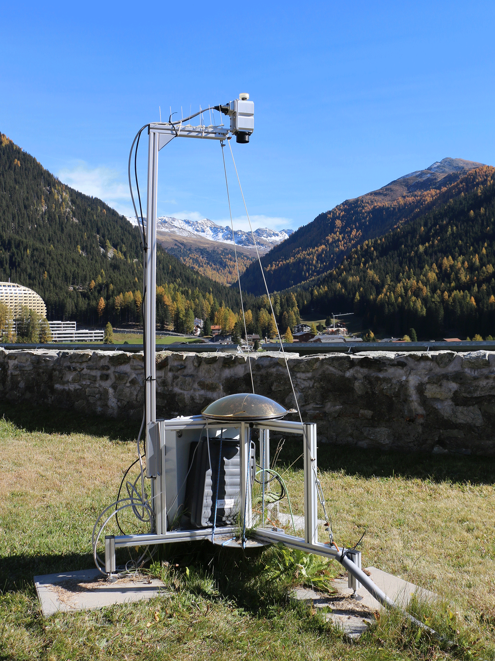
Figure 1The infrared cloud camera (IRCCAM) in the measurement enclosure of PMOD/WRC in Davos, Switzerland.
The camera of the IRCCAM was calibrated in the PMOD/WRC laboratory in order to determine the brightness temperature or the absolute radiance in Wm−2 sr−1 for every pixel in an IRCCAM image. The absolute calibration was obtained by placing the camera in front of the aperture of a well-characterised black body at a range of known temperatures between −20 and +20 ∘C in steps of 5 ∘C (Gröbner, 2008). The radiance emitted by a black-body radiator can be calculated using the Planck radiation formula,
where T is the temperature, λ the wavelength, h is the Planck constant, Js, c the speed of light, 299 792 458 ms−1 and k the Boltzmann constant, J K−1. For the IRCCAM camera, the spectral response function Rλ as provided by the manufacturer is shown in Fig. 2 and is used to calculate the integrated radiance LR,
where T is the effective temperature of the black body (Gröbner, 2008) and LR is the integrated radiance measured by the IRCCAM camera. To retrieve the brightness temperature (TB) from the integrated radiance LR, Eq. (2) cannot be solved analytically. Therefore, as an approximation, we are using a polynomial function TB=f(LR) to retrieve the brightness temperature TB from the radiance LR. Using Eq. (2), LR values are calculated for temperatures in the range of −40 and +40 ∘C. The resulting fitting function is a polynomial third-order function (see Fig. 3), which is used to retrieve TB from the integrated radiance LR for every pixel in an IRCCAM image.
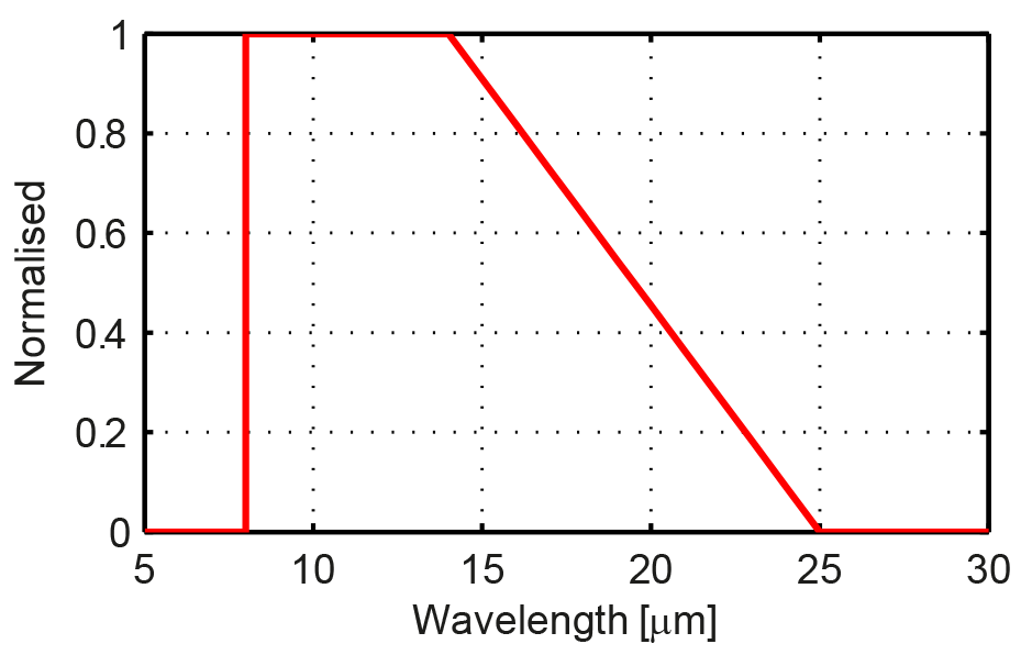
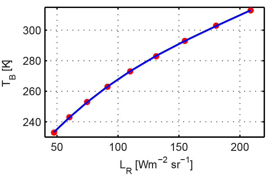
Figure 3Brightness temperature TB versus integrated radiance LR for different radiance values (red dots), and the corresponding third-order polynomial fitting function (blue line).
The IRCCAM calibration in the black-body aperture was performed on 16 March 2016 and all its images are calibrated with the corresponding calibration function retrieved from the laboratory measurements. The calibration uncertainty of the camera in terms of brightness temperatures (in a range of −40 and +40 ∘C) is estimated at 1 K for a Planck spectrum as emitted by a black-body radiator. Furthermore, a temperature correction function for the camera was derived from these laboratory calibrations in order to correct the measurements obtained at ambient temperatures outdoors. The hemispherical sky images taken by the IRCCAM are converted to polar coordinates (Θ, Φ) for the purpose of retrieving brightness temperatures in dependence of zenith and azimuth. Due to slight aberrations in the optical system of the IRCCAM, the Θ coordinate does not follow a linear relationship with the sky zenith angle, producing a distorted sky image. Therefore, a correction function was determined by correlating the apparent solar position as measured by the IRCCAM with the true solar position obtained by a solar position algorithm. This correction function was then applied to the raw camera images to obtain undistorted images of the sky hemisphere.
One should note that observing the sun with the Gobi camera implies that the spectral filter used in the camera to limit the spectral sensitivity to the 8–14 µm wavelength band has some leakage at shorter wavelengths. Fortunately, this leakage is confined to a narrow region around the solar disk (around 1∘) as shown in Fig. 4. Thus, it has no effect on the remaining part of the sky images taken by the IRCCAM during daytime measurements.
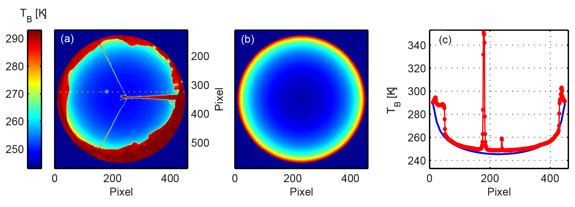
Figure 4(a) Measured brightness temperature (TB) on the cloud-free day 18 June 2017, 10:49 UTC (SZA = 24∘), (b) the corresponding modelled brightness temperature and (c) the measured (red) and modelled (blue) profile of the sky brightness temperature along one azimuth position (shown as a yellow line in a).
The main objective of the IRCCAM study is to determine cloud properties from the measured sky radiance distributions. The cloudy pixels in every image are determined from their observed higher radiances with respect to that of a cloud-free sky. The clear-sky radiance distributions are determined from radiative transfer calculations using MODTRAN 5.1 (Berk et al., 2005), using as input parameters screen-level air temperature and integrated water vapour (IWV). The temperature was determined at 2 m elevation from a nearby SwissMetNet station, while the IWV was retrieved from GPS signals operated by the Federal Office for Topography and archived in the Studies in Atmospheric Radiation Transfer and Water Vapour Effects (STARTWAVE) database hosted at the Institute of Applied Physics at the University of Bern (Morland et al., 2006). For practical reasons, a look-up table (LUT) for a range of temperatures and IWV was generated, which was then used to compute the reference clear-sky radiance distribution for every single image taken by the camera. A similar approach that is used to detect cloud patterns is described in Bertin et al. (2015a) and Liandrat et al. (2017).
The sky brightness temperature distribution as measured on a cloud-free day (18 June 2017, 10:49 UTC) and the corresponding modelled sky brightness temperature are shown in Fig. 4a and b. As expected, the lowest radiance is emitted at the zenith, with a gradual increase at increasing zenith angle, until the measured effective sky brightness temperature at the horizon is nearly equal to ambient air temperature (Smith and Toumi, 2008). Figure 4c shows the profiles of the measured (red) and modelled (blue) brightness temperatures along one azimuth position going through the solar position (yellow line in Fig. 4a). As can be seen in Fig. 4c, the measured and modelled sky distributions agree fairly well, with large deviations at high zenith angles due to the mountains obstructing the horizon around Davos. The short-wave leakage from the sun can also be clearly seen around pixel number 180. A smaller deviation is seen at pixel number 239 from the wires holding the frame of the camera.
The average difference between the measured and modelled clear-sky radiance distributions was determined for several clear-sky days during the measurement period in order to use that information when retrieving clouds from the IRCCAM images. Differences can arise, on the one hand, from the rather crude radiative transfer modelling, which only uses surface temperature and IWV as input parameters to the model. On the other hand, it can arise from instrumental effects such as a calibration uncertainty of ±1 K. An effect of the mirror temperature and a possible mismatch between actual and nominal spectral response functions of the IRCCAM camera are other potential causes for this difference. However, both of these possible effects have not been taken into account. The validation measurements span 8 days, with full-sky measurements obtained every minute, yielding a total of 11 512 images for the analysis. For every image, the corresponding sky radiance distribution was calculated from the LUT, as shown in Fig. 4b. The residuals between the measured and modelled sky radiance distributions were calculated by averaging over all data points with zenith angles smaller than 60∘ while removing the elements (frame and wires) of the IRCCAM within the FOV of the camera, resulting in one value per image. The brightness temperature differences between IRCCAM and model calculations show a mean difference of +4.0 K and a standard deviation of 2.4 K over the whole time period. The observed variability comes equally from day-to-day variations as well as from variations within a single day. No systematic differences are observed between day and night-time data.
The stability of the camera over the measurement period is investigated by comparing the horizon brightness temperature derived from the IRCCAM with the ambient air temperature measured at the nearby SwissMetNet station. As mentioned by Smith and Toumi (2008), the horizon brightness temperature derived from the IRCCAM should approach the surface air temperature close to the horizon. Indeed, the average difference between the horizon brightness temperature derived from the IRCCAM and the surface air temperature was 0.1 K with a standard deviation of 2.4 K, showing no drifts over the measurement period and thus confirming the high stability of the IRCCAM during this period. The good agreement of 0.1 K between the derived horizon brightness temperature from the IRCCAM and the surface air temperature confirms the absolute calibration uncertainty of ±1 K of the IRCCAM. Therefore, the observed discrepancy of 4 K between measurements and model calculations mentioned previously can probably be attributed to the uncertainties in the model parameters (temperature and IWV) used to produce the LUT.
2.1.1 Cloud detection algorithm
After setting up the IRCCAM, a horizon mask is created initially to determine the area of the IRCCAM image representing the sky hemisphere. A cloud-free image is selected manually. The sky area is selected by the very low sky brightness temperatures with respect to the local obstructions with much larger brightness temperatures. This image mask contains local obstructions such as the IRCCAM frame (camera, arm and wire ropes) as well as the horizon, which, in the case of Davos, consists of mountains limiting the FOV of the IRCCAM. Thereafter, the same horizon mask is applied to all IRCCAM images. The total number of pixels within the mask is used as a reference and the cloud fraction is defined as the number of pixels detected as cloudy relative to the total number.
The algorithm used to determine cloudy pixels from an IRCCAM image consists of two parts. The first part uses the clear-sky model calculations as a reference to retrieve low- to mid-level clouds. These clouds have large temperature differences compared to the clear-sky reference. In this part of the algorithm, cloudy pixels are defined for measured sky brightness temperatures that are at least 6.5 K greater than the modelled clear-sky reference value. A rather large threshold value was empirically chosen to avoid any erroneous clear-sky misclassifications as cloudy pixels. The thinner and higher clouds with lower brightness temperatures are therefore left for the second part of the algorithm.
In order to determine the thin and high-level clouds within an IRCCAM image, non-cloudy pixels remaining from the first part of the algorithm are used to fit an empirical clear-sky brightness temperature as a function of the zenith angle,
where TB is the brightness temperature for a given zenith angle Θ, and T65, a and b are the retrieved function parameters (Smith and Toumi, 2008). This second part of the algorithm assumes a smooth variation of the clear-sky brightness temperature with zenith angle. Thereby, it determines cloudy pixels as deviations from this smooth function as well as requiring a brightness temperature higher than this empirical clear-sky reference. Pixels with a brightness temperature higher than the empirically defined threshold of 1.2 K are defined as cloudy and removed from the clear-sky data set. This procedure is repeated up to 10 times to iteratively find pixels with a brightness temperature higher than the clear-sky function. One restriction of this fitting method is that it requires at least broken cloud conditions, as it does not work well under fully overcast conditions without the presence of cloud-free pixels to constrain the fitting procedure.
The selected threshold of 1.2 K allows the detection of low-emissivity clouds, but still misses the detection of parts of thin, high-level cirrus clouds even though they can be clearly seen in the IRCCAM images. Unfortunately, reducing the threshold to less than 1.2 K results in many clear-sky misclassifications as clouds. Therefore, under these conditions, it seems that using a spatial smoothness function is not sufficient to infer that individual pixels are cloudy; a more advanced algorithm as discussed in Brocard et al. (2011) is required to define clouds, not only on a pixel-by-pixel basis but as a continuous structure (e.g. pattern recognition algorithm).
Before reaching the final fractional cloud data set, some data-filtering procedures are applied: situations with precipitation are removed by considering precipitation measurements from the nearby SwissMetNet station; ice or snow deposition on the IRCCAM mirror is detected by comparing the median radiance of a sky area with the median radiance value of an area on the image showing the frame of the IRCCAM. In cases where the difference between the median values of the two areas is smaller than the empirically defined value of 5 Wm−2 sr−1, the mirror is assumed to be contaminated by snow or ice and therefore does not reflect the sky, so the image is excluded. The horizon mask does not cover all pixels that do not depict sky, which leads to an offset in the calculated cloud fraction of around 0.04. This offset is removed before comparing the cloud fraction determined by the IRCCAM with other instruments.
2.2 Mobotix camera
A commercial surveillance Q24M camera from Mobotix (https://www.mobotix.com/, last access: 22 September 2018) was installed in Davos in 2011. The camera has a fisheye lens and is sensitive in the red–green–blue (RGB) wavelength range. The camera takes images from the whole of the upper hemisphere with a spatial resolution of 1200×1600 pixels. The camera system is heated, ventilated and installed on a solar tracker with a shading disk. The shading disk avoids overexposed images due to the sun. The time resolution of the Mobotix data is 1 min (from sunrise to sunset) and the exposure time is 1∕500 s.
An algorithm determines the cloud fraction of each image automatically (Aebi et al., 2017; Wacker et al., 2015). Before applying the cloud detection algorithm, the images are preprocessed. The distortion of the images is removed by applying a correction function. The same horizon mask, which was defined on the basis of a cloud-free image, is applied to all images. After this preprocessing, the colour ratio (the sum of the blue to green ratio plus the blue to red ratio) is calculated per pixel. To perform the cloud determination per pixel, this calculated colour ratio is compared to an empirically defined reference ratio value of 2.2. Comparing the calculated colour ratio value with this reference value designates whether a pixel is classified as cloudy or as cloud-free. The cloud fraction is calculated by the sum of all cloud pixels divided by the total number of sky pixels.
The cloud classes are determined with a slightly adapted algorithm from Heinle et al. (2010) which is based on statistical features (Wacker et al., 2015; Aebi et al., 2017). The cloud classes determined are stratocumulus (Sc), cumulus (Cu), stratus–altostratus (St–As), cumulonimbus–nimbostratus (Cb–Ns), cirrocumulus–altocumulus (Cc–Ac), cirrus–cirrostratus (Ci–Cs) and cloud-free (Cf).
2.3 Schreder camera
The total-sky camera VIS-J1006 from Schreder (http://www.schreder-cms.com/en/, last access: 22 September 2018) consists of a digital camera with a fisheye lens. The VIS-J1006 Schreder camera is sensitive in the RGB region of the spectrum and takes two images every minute with different exposure times (1∕500 and 1∕1600 s). The aperture is fixed at f∕8 for both images. The resolution of the images is 1200×1600 pixels. The camera comes equipped with a weatherproof housing and a ventilation system.
The images from the Schreder camera are analysed using two different algorithms. The original software is directly delivered from the company Schreder. Before calculating the fractional cloud coverage, some steps are needed to define the settings that are needed to preprocess the images. In a first step, the centre of the image is defined manually. In a second step, the maximum zenith angle of the area taken into account for further analyses is defined. Unfortunately, the maximum possible zenith angle is only 70∘ and thus a larger fraction of the sky cannot be analysed. After the distortion of the images is removed, in a fourth step a horizon mask is defined on the basis of a cloud-free image. The mask also excludes the pixels around the sun. In a last step, a threshold is defined which specifies whether a pixel is classified as a cloud or not. The settings from these preprocessing steps are then applied to all images from the Schreder camera. In the following, the term Schreder refers to data for which this algorithm is used.
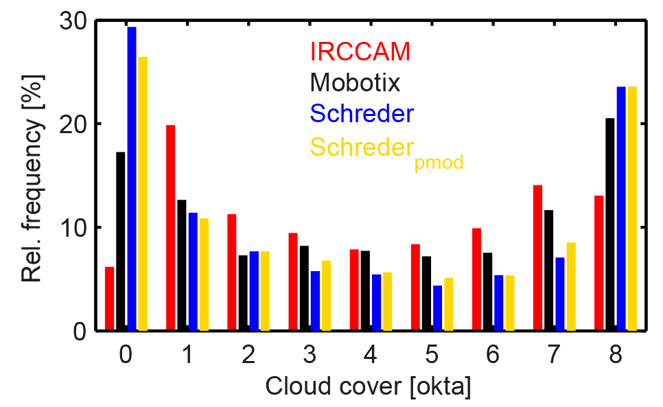
Figure 5Relative frequencies of the determined cloud coverage of the analysed instruments for selected bins of cloud coverage at Davos (during daytime). Zero okta: 0–0.0500, 1 okta: 0.0500–0.1875, 2 oktas: 0.1875–0.3125, 3 oktas: 0.3125–0.4375, 4 oktas: 0.4375–0.5625, 5 oktas: 0.5625–0.6875, 6 oktas: 0.6875–0.8125, 7 oktas: 0.8125–0.9500, 8 oktas: 0.9500–1.
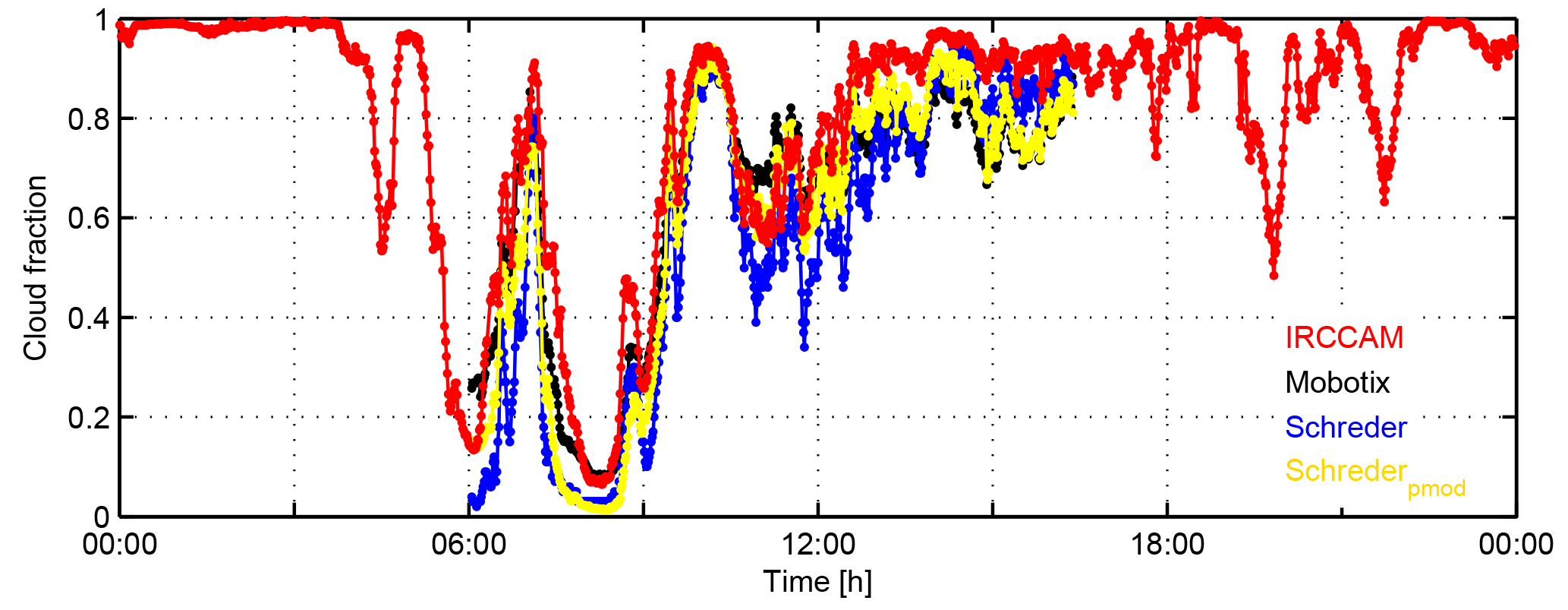
Figure 6Cloud fraction determined by the analysed cameras and algorithms (red is IRCCAM, black is Mobotix, blue is Schreder, yellow is Schrederpmod) on 4 April 2016.
Due to the Schreder algorithm's limitation of a maximum zenith angle of 70∘, we used the same algorithm as for the Mobotix camera, referred to hereafter as Schrederpmod. The algorithm Schrederpmod has the advantage that the whole of the upper hemisphere is considered when calculating the fractional cloud coverage. Thus, a new horizon mask is defined on the basis of a cloud-free image. The colour ratio reference that distinguishes between clouds and no clouds is assigned an empirical value of 2.5, which is slightly different to that used for the Mobotix camera. The Schreder camera in Davos has been measuring continuously since March 2016.
2.4 APCADA
The automated partial cloud amount detection algorithm (APCADA) determines the cloud amount in oktas using downward long-wave radiation from pyrgeometers, temperature and relative humidity measured at screen-level height (Dürr and Philipona, 2004). APCADA is only able to detect low- and mid-level clouds and is not sensitive to high-level clouds. The time resolution of APCADA is 10 min during daytime and night-time. The agreement of APCADA compared to synoptic observations at high-altitude and midlatitude stations, such as Davos, is that 82 % to 87 % of cases during daytime and night-time have a maximum difference of ±1 okta (±0.125 cloud fraction) and between 90 % to 95 % of cases have a difference of ±2 oktas (±0.250 cloud fraction) (Dürr and Philipona, 2004).
In order to compare the cloud coverage information retrieved from APCADA with the fractional cloud coverages retrieved from the cameras, the okta values are converted to fractional cloud coverage values by multiplying the okta values by 0.125. In the current study, APCADA is mainly used for comparisons of the night-time IRCCAM data.
In the aforementioned time period 21 September 2015 to 30 September 2017, the IRCCAM data set comprises cloud cover information from 581 730 images. The Mobotix data set comprises 242 249 images (because only daytime data are available) and the Schreder data set 184 746 images (shorter time period and also only daytime). Figure 5 shows the relative frequencies of cloud cover detection from the different camera systems in okta bins during the daytime and when all camera data are available. Zero okta corresponds to a cloud fraction of 0 to 0.05 and 8 oktas to a cloud fraction of 0.95 to 1. One and seven oktas correspond to intermediate bins of 0.1375 cloud fraction and oktas two to six to intermediate bins of 0.125 cloud fraction (Wacker et al., 2015). Cloud-free (0 okta) and overcast (8 oktas) are the cloud coverages that are most often detected in the aforementioned time period. This behaviour also agrees with the analysis of the occurrence of fractional cloud coverages over a longer time period in Davos discussed in Aebi et al. (2017). All four instruments and algorithms show similar relative occurrences of cloud coverage of 2–6 oktas. It is noteworthy that the IRCCAM clearly underestimates the occurrence of 0 oktas in comparison to the cameras measuring in the visible spectrum (by up to 20 %). On the other hand, the relative frequency of the IRCCAM of 1 okta is clearly larger (by up to 10 %) compared to the visible cameras. This can be explained by higher brightness temperatures measured in the vicinity of the horizon above Davos. These higher measured brightness temperatures are falsely determined as cloudy pixels (up to 0.16 cloud fraction). Since these situations with larger brightness temperatures occur quite frequently, the IRCCAM algorithm more often detects cloud coverages of 1 okta instead of 0 okta. Also, at the other end of the scale, the IRCCAM detects slightly larger values of a relative frequency of 7 oktas compared to the visible cameras and slightly lower relative frequencies of a measurement of 8 oktas.

Figure 7The cloud situation on 4 April 2016 10:00 UTC (a) on an image from Mobotix and the cloud fraction determined from (b) IRCCAM (temperature range from 244 K (blue) to 274 K (yellow)) and (c) Mobotix (white: clouds, blue: cloud-free, yellow: area around sun).
As an example, Fig. 6 shows the cloud fraction determined on 4 April 2016, where various cloud types and cloud fractions were present. This day starts with an overcast sky and precipitation and therefore the IRCCAM measures fractional cloud coverages of more than 0.98. The cloud layer disperses until it reaches cloud fraction values of 0.1 at around 06:00 UTC. At this time the sun rises above the effective horizon and the visible all-sky cameras start to measure shortly thereafter. The cloud classes are determined with the algorithm developed by Wacker et al. (2015) based on Mobotix images. In the early morning, the cloud type present is cumulus. The larger difference of more than 0.1 between the cloud fraction determined by the Schreder algorithm and the other algorithms can be explained after a visual observation of the image: the few clouds that are present are located close to the horizon and thus in the region of the sky that the Schreder algorithm is not able to analyse. The fractional cloud coverage increases again to values of around 0.8 at 07:00 UTC. At this time, all four cameras and algorithms determine a similar fractional cloud coverage. Around 08:00 UTC a first cirrostratus layer appears, which is slightly better detected by the IRCCAM and the Mobotix algorithm than by the two algorithms using the Schreder images. Two hours later, around 10:00 UTC, the main cloud type present is again cumulus. Low-level clouds are quite precisely detected by all camera systems and thus, in this situation, the maximum observed difference is only 0.06. Figure 7a shows exactly this situation as an RGB image taken by the Mobotix camera, and the corresponding classifications as cloudy or non-cloudy pixels determined by the IRCCAM (Fig. 7b) and by the Mobotix algorithm (Fig. 7c). From 11:00 UTC onwards the cumulus clouds are found in the vicinity of the horizon and cirrus–cirrostratus closer to the zenith. Because all algorithms have difficulty detecting thin and high-level clouds, the differences in the determined cloud fractions are variable. Again, the Schreder algorithm is not able to analyse the cloud fraction near the horizon and thus it always detects the smallest fraction compared to the other algorithms. The visible cameras continue measuring until 16:23 UTC when the sun sets, and afterwards only data from the IRCCAM are available.
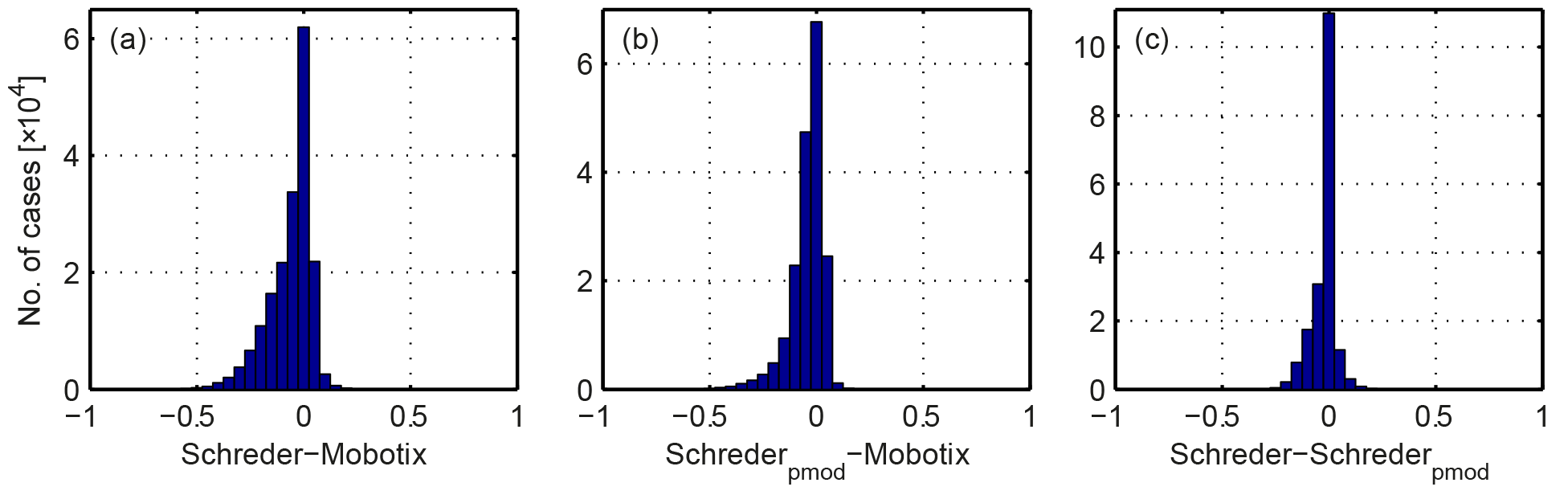
Figure 8Residuals of the comparison of cloud fraction retrieved from the visible cameras and algorithms used in the study: (a) Schreder-Mobotix, (b) Schrederpmod-Mobotix and (c) Schreder–Schrederpmod.

Figure 9Residuals of the comparison of cloud fraction retrieved from the IRCCAM versus cloud fraction retrieved from the visible cameras: (a) IRCCAM–Mobotix, (b) IRCCAM–Schreder and (c) IRCCAM–Schrederpmod.
3.1 Visible all-sky cameras
Before validating the fractional cloud coverage determined by the IRCCAM algorithm, the fractional cloud coverages, which are determined using the images of the visible all-sky cameras Mobotix and Schreder, are compared with each other to gain a better understanding of their performance. The time period analysed here is 9 March 2016 to 30 September 2017, consisting of only daytime data, which correspond to a data set of 184 746 images. Additionally, the results from the visible all-sky cameras are compared with data retrieved from APCADA (temporal resolution of 10 min). For this comparison, 32 902 Mobotix and 24 907 Schreder images are considered.
The histograms of the residuals of the difference in the cloud fractions (range between [−1;1]) between the visible all-sky cameras are shown in Fig. 8 and the corresponding median and 5th and 95th percentiles are shown in Table 1.
Table 1Median and 5th and 95th percentiles of the differences in calculated cloud fractions from the visible all-sky cameras and APCADA. The numbers are in the range [-1;1].
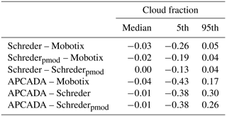
As shown in Table 1, the two algorithms from the Schreder camera as well as APCADA underestimate the cloud fraction determined from Mobotix images, with a maximum median difference of −0.04. Although the median difference in cloud fraction between the two Schreder algorithms is 0.00, the distribution tends towards more negative values. This more pronounced underestimation of fractional cloud coverage of the Schreder algorithm might be explained by the smaller fraction of the sky being analysed (Fig. 8c). The underestimation in the retrieved cloud fraction of the Schreder algorithm for 90 % of the data is even slightly larger in comparison to the cloud fraction determined with the Mobotix algorithm. The spread (shown as 5th and 95th percentiles in Table 1) is greatest for all comparisons of the algorithms from the visible cameras with APCADA. As previously mentioned in Sect. 2.4, APCADA gives the cloud fraction only in steps of 0.125, and it is thus not as accurate as the cloud fraction determined from the cameras. This fact might explain the large variability in the residuals.
In Fig. 8 it is shown that the distribution of the residuals between the cloud fraction retrieved from Mobotix versus the cloud fraction retrieved from the two Schreder algorithms (Fig. 8a and b) are left-skewed, which confirms that the cloud fraction retrieved from the two Schreder algorithms underestimates the cloud fraction retrieved from the Mobotix images.
Taking the measurement uncertainty of human observers and also of other cloud detection instruments to be ±1 okta to ±2 oktas (Boers et al., 2010), we consider this to be a baseline uncertainty range that tests the performance in the detection of cloud fraction of our visible camera systems. The algorithms for the visible camera systems determine the cloud fraction for 94 %–100 % of the data within ±2 oktas (±0.25) and for 77 %–94 % of the data within ±1 okta (±0.125). Comparing the cloud fraction determined from APCADA with the cloud fraction determined from the visible cameras shows that in only 67 %–71 % of the cases is there an agreement of ±1 okta (±0.125) and in 83 %–86 % of data an agreement of ±2 oktas (±0.25). All of these results are further discussed in the next section.
3.2 IRCCAM validation
As described in Sect. 3.1, in up to 94 % of the data set the visible cameras are consistent to within ±1 okta (±0.125) in the cloud fraction detection, so that they can be used to validate the fractional cloud coverage determined by the IRCCAM. For this comparison, a data set of 242 249 images (Mobotix) and a data set of 184 746 images (Schreder) are available. This comparison is only performed for daytime data of the IRCCAM, because from the visible cameras only daytime data are available.
Table 2Median and 5th and 95th percentiles of the differences in calculated cloud fractions between IRCCAM and the visible all-sky cameras. The numbers are in the range [-1;1].
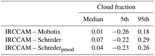
The residuals and some statistical values of the differences between the IRCCAM and the visible cameras are shown in Fig. 9 and Table 2. With a median value of 0.01, there is no considerable difference between the cloud fraction determined by the IRCCAM and the cloud fraction determined by the Mobotix camera. The differences between the IRCCAM and the Schreder algorithms are only slightly larger, with median values of 0.04 and 0.07 for Schrederpmod and Schreder. Thus, the IRCCAM only marginally overestimates the cloud fraction in comparison to the cloud fraction determined by the visible cameras. The distributions of the residuals IRCCAM–Schreder and IRCCAM–Schrederpmod are quite symmetrical (Fig. 9b and c). The distribution of the residuals in the cloud fraction IRCCAM–Mobotix is slightly left-skewed (Fig. 9a).
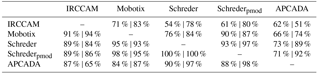
Table 3Percentage of fractional cloud coverage data which agree within ±1 okta (all values above the main diagonal) and ±2 oktas (all values below the main diagonal) when comparing two algorithms.
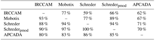
The percentage of agreement in the determined cloud fraction between the sky cameras and APCADA separately is given in Table 3. All values above the main diagonal designate the fraction of data that agree within ±0.125 (±1 okta) fractional cloud coverage between two individual algorithms and all values below the main diagonal indicate the fraction that agree within ±0.25 (±2 oktas) cloud fraction. The agreement of the IRCCAM in comparison with different visible all-sky cameras and APCADA is that 59 %–77 % of the IRCCAM data are within ±0.125 (±1 okta) fractional cloud coverage and 80 %–93 % of the data are within ±0.25 (±2 oktas) fractional cloud coverage. These values of the IRCCAM are only slightly lower than the agreement that the visible cameras have with each other (94 %–100 % and 77 %–94 % are within ±2 oktas and ±1 okta respectively). The close agreement between the two algorithms Schreder and Schrederpmod is noteworthy, although they analyse a different number of image pixels. We can conclude that the IRCCAM retrieves cloud fraction values within the uncertainty range of the cloud fraction retrieved from the visible cameras and also in a similar range to state-of-the-art cloud detection instruments.
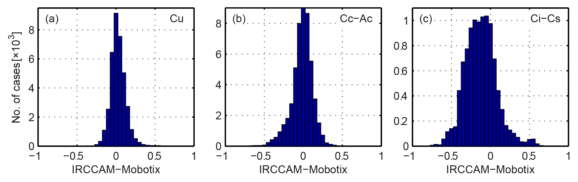
Figure 10Residuals of the comparison of cloud fraction determined from IRCCAM images versus cloud fraction determined from Mobotix images for the following cloud classes: (a) Cu is cumulus, (b) Cc–Ac is cirrocumulus–altocumulus and (c) Ci–Cs is cirrus–cirrostratus.
3.2.1 Cloud class analysis
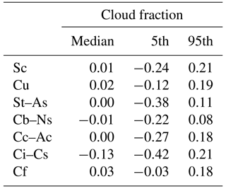
Although the median difference between the cloud fraction determined with the IRCCAM algorithm and the cloud fraction determined with the Mobotix algorithm is not evident, it is interesting to analyse differences in cloud fraction depending on the cloud type. The algorithm developed by Wacker et al. (2015) is used to distinguish six selected cloud classes and cloud-free cases automatically on the basis of the Mobotix images. Figure 10 shows the distribution of the residuals of the cloud fraction of the two aforementioned algorithms for (a) cumulus (low-level; N= 37 320), (b) cirrocumulus–altocumulus (mid-level; N= 52 097) and (c) cirrus–cirrostratus (high-level; N= 10 467). The median value of the difference in cloud fraction between IRCCAM and Mobotix for Cu clouds is 0.02 and therefore not considerable. In general, all low-level clouds (Sc, Cu, St–As, Cb–Ns) are detected with a median cloud fraction difference of −0.01 to 0.02 (Table 4). The IRCCAM and the Mobotix camera observe the mid-level cloud class Cc–Ac with a median agreement of cloud fraction of 0.00 but with a slightly asymmetric distribution towards negative values. Considering 90 % of the data set of Cc–Ac clouds, the IRCCAM tends to underestimate the cloud fraction for the mid-level cloud class. The spread in the Cc–Ac data (shown as 5th and 95th percentiles in Table 4) is in general slightly larger than that for low-level clouds. The median value of the cloud fraction residuals determined on the basis of IRCCAM images and those based on Mobotix images for the high-level cloud class Ci–Cs is, at −0.13, clearly larger in comparison to clouds at lower levels. Thus, although we applied the second part of the algorithm to detect thin, high-level clouds from the IRCCAM images, it still misses a large fraction of the Ci–Cs clouds in comparison to the Mobotix camera. The distribution of the residuals (Fig. 10c) is clearly wider, which leads to 5th and 95th percentiles of −0.42 and 0.21. Due to the large spread and as shown in Aebi et al. (2017), the visible camera systems also have difficulties in detecting the thin, high-level clouds.
Table 4Median and 5th and 95th percentiles of the differences in calculated cloud fractions from IRCCAM and Mobotix images for selected cloud classes: stratocumulus (Sc), cumulus (Cu), stratus–altostratus (St–As), cumulonimbus–nimbostratus (Cb–Ns), cirrocumulus–altocumulus (Cc–Ac), cirrus–cirrostratus (Ci–Cs) and cloud-free (Cf). The numbers are in the range [-1;1].
3.2.2 Day–night differences
Table 5Median and 5th and 95th percentiles of the differences in calculated cloud fractions from IRCCAM versus APCADA: overall, daytime only and night-time only. The numbers are in the range [-1;1].
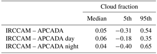
Table 6Identical to Table 3, but on the left are the values for the summer months (June, July, August) and on the right are the values for the winter months (December, January, February).
So far, only daytime data have been analysed. At PMOD/WRC in Davos, during night-time the cloud fraction is retrieved from pyrgeometers as well as from the IRCCAM. Therefore the IRCCAM cloud coverage data are compared with the data retrieved from the APCADA, which uses pyrgeometer data and calculates cloud fractions independently of the time of day. As explained in Sect. 2.4, APCADA only determines the cloud fraction from low- to mid-level clouds and gives no information about high-level clouds. It also gives the cloud fraction only in okta steps (equals steps of 0.125 cloud fraction).
Table 5 shows the median values of the residuals of the cloud fraction between IRCCAM and APCADA for all available data (N= 103 624), only daytime data (N= 32 902) and only night-time data (N= 70 722) and the corresponding 5th and 95th percentiles separately. The overall median difference value in cloud fraction detection between IRCCAM and APCADA is, at 0.05, in a similar range to the ones for the comparison of the cloud fraction determined with the cloud cameras. The median value for daytime data is, at 0.06, only slightly larger than the one for night-time data (0.04). However, the spread of the residuals is notably broad, mainly during night-time with a large positive 95th percentile value (0.65). However, because APCADA already showed larger spreads in the residuals in comparison to the fractional cloud coverage determined with the visible all-sky cameras, it is not possible to draw the conclusion that the IRCCAM overestimates the cloud fraction at night-time.
3.2.3 Seasonal variations
The seasonal analysis is performed in order to investigate whether a slightly unequal distribution of cloud types in different months in Davos (Aebi et al., 2017) has an impact on the performance of the cloud fraction retrieval between seasons. The percentage of agreement in the retrieved cloud fraction between the systems is again given for a maximum of ±1 okta (±0.125) differences (top) and ±2 oktas (±0.25) differences (bottom) for summer (left values) and winter (right values) in Table 6. For all algorithms there is a slightly closer agreement in the determined cloud fraction in the winter months in comparison to the summer months. In winter, the IRCCAM agrees with the other cameras in 78 %–83 % of the data within ±0.125 (±1 okta) and as high as 84 %–94 % within ±0.25 (±2 oktas). In summer, the agreement in cloud fraction is only 54 %–71 % of the data within ±0.125 (±1 okta) cloud fraction, but nevertheless, 89 %–91 % of values fall within ±0.25 (±2 oktas) cloud fraction. The slight difference between the two seasons might be explained by the slightly larger frequency of occurrence of the thin and low-emissivity cloud class cirrocumulus–altocumulus in Davos in summer than in winter (Aebi et al., 2017). Also, the values for spring (MAM) and autumn (SON) are in a similar range to the ones for summer and winter. Thus, the IRCCAM (and also the other camera systems) do not show any noteworthy variation in any of the seasons.
The current study describes a newly developed instrument – the thermal infrared cloud camera (IRCCAM) and its algorithm – that determines cloud fraction on the basis of absolute sky radiance distributions. The cloud fraction determined on the basis of IRCCAM images is compared with the cloud fraction determined on the basis of images from two visible camera systems (one analysed with two different algorithms) and with the partial cloud amount determined with APCADA.
The overall median differences between the determined cloud fraction from the IRCCAM and the fractional cloud coverage determined from other instruments and algorithms are 0.01–0.07 fractional cloud coverage. The IRCCAM has an agreement of ±2 oktas (±0.25) in more than 90 % of cases and an agreement of ±1 okta (±0.125) in up to 77 % of the cases in comparison to other instruments. Thus, in only 10 % of the data, the IRCCAM typically overestimates the cloud fraction in comparison with the cloud fraction determined from the all-sky cameras sensitive in the visible region of the spectrum. Differences in the cloud fraction estimates can be due to different thresholds for the camera systems (as discussed in Calbó et al., 2017) as well as some other issues addressed throughout the current study.
In general, there is no considerable difference in the performance of the IRCCAM in the different seasons. Analysis of the median values of the residuals between the cloud fraction determined from the IRCCAM and the ones calculated from APCADA shows no difference between daytime and night-time, even though the spread of the residuals is clearly higher during night-time.
The cloud fraction determination of the three cameras is independent of cloud classes, with the exception of thin cirrus clouds, which are underestimated by the current IRCCAM algorithm by about 0.13 cloud fraction.
Overall, the IRCCAM is able to determine cloud fraction with good agreement in comparison to all-sky cameras sensitive in the visible spectrum and with no considerable differences in its performance during different times of the day or in different seasons. Thus, the IRCCAM is a stable system that can be used throughout the day and night with a high temporal resolution. In comparison to other state-of-the-art cloud detection instruments (e.g. ceilometer or NubiScope) it has the advantage of measuring the whole of the upper hemisphere at one specific moment. Its accuracy ranges from similar to rather better than that of the NubiScope (Feister et al., 2010) as well as that of the human observers (Boers et al., 2010).
In this study we mainly showed one application of the IRCCAM, which is to retrieve fractional cloud coverage information from the images. However, the known brightness temperature distribution of the sky and thus the known radiance can also be used for other applications, including the determination of other cloud parameters (cloud type, cloud level, cloud optical thickness) as well as the retrieval of information about downward long-wave radiation in general. Thus, after some improvements in the hardware (e.g. a heating or ventilation system to avoid a frozen mirror) and software (improvements of the cloud algorithm detecting low-emissivity clouds, e.g. by pattern recognition) the IRCCAM might be of interest for a number of further applications, for example, at meteorological stations or airports.
Data are available from the corresponding author on request.
The authors declare that they have no conflict of interest.
This research was carried out within the framework of the project “A
Comprehensive Radiation Flux Assessment (CRUX)” financed by MeteoSwiss. The
project was funded in autumn 2013. The authors thank the three referees for
their constructive comments.
Edited by:
Manfred Wendisch
Reviewed by: Josep Calbó, Pascal Kuhn, and one anonymous referee
Ackerman, S. A., Holz, R. E., Frey, R., Eloranta, E. W., Maddux, B. C., and McGill, M.: Cloud Detection with MODIS. Part II: Validation, J. Atmos. Ocean. Tech., 25, 1073–1086, https://doi.org/10.1175/2007JTECHA1053.1, 2008. a, b
Aebi, C., Gröbner, J., Soder, R., Schlatter, P., and Dürig, F.: Development of thermal infrared cloud camera (IRCCAM), Annual Report, PMOD/WRC, 2014. a
Aebi, C., Gröbner, J., Kämpfer, N., and Vuilleumier, L.: Cloud radiative effect, cloud fraction and cloud type at two stations in Switzerland using hemispherical sky cameras, Atmos. Meas. Tech., 10, 4587–4600, https://doi.org/10.5194/amt-10-4587-2017, 2017. a, b, c, d, e
Baum, B. A. and Platnick, S.: Introduction to MODIS Cloud Products, in: Earth Science Satellite Remote Sensing, Springer, Berlin, Heidelberg, 2006. a
Berger, L., Besnard, T., Genkova, I., Gillotay, D., Long, C., Zanghi, F., Deslondes, J. P., and Perdereau, G.: Image comparison from two cloud cover sensor in infrared and visible spectral regions, in: 21st International Conference on Interactive Information Processing Systems (IIPS) for Meteorology, Oceanography, and Hydrology, available at: https://ams.confex.com/ams/Annual2005/techprogram/paper_83438.htm (last access: 22 September 2018), 2005. a
Berk, A., Anderson, G. P., Acharya, P. K., Bernstein, L. S., Muratov, L., Lee, J., Fox, M. J., Adler-Golden, S. M., Chetwynd, J. H., Hoke, M. L., Lockwood, R. B., Cooley, T. W., and Gardner, J. A.: MODTRAN5: a reformulated atmospheric band model with auxiliary species and practical multiple scattering options, Proc. SPIE, 5655, 88–95, https://doi.org/10.1117/12.578758, 2005. a
Bertin, C., Cros, S., Saint-Antonin, L., and Schmutz, N.: Prediction of optical communication link availability: real-time observation of cloud patterns using a ground-based thermal infrared camera, Proc. SPIE, 9641, 96410A, https://doi.org/10.1117/12.2194920, 2015a. a, b
Bertin, C., Cros, S., Schmutz, N., Liandrat, O., Sebastien, N., and Lalire, S.: Detection unit and method for identifying and monitoring clouds in an observed area of the sky, Patent EP3198311, 2015b. a
Boers, R., de Haij, M. J., Wauben, W. M. F., Baltink, H. K., van Ulft, L. H., Savenije, M., and Long, C. N.: Optimized fractional cloudiness determination from five ground-based remote sensing techniques, J. Geophys. Res.-Atmos., 115, d24116, https://doi.org/10.1029/2010JD014661, 2010. a, b, c, d, e, f
Brede, B., Thies, B., Bendix, J., and Feister, U.: Spatiotemporal High-Resolution Cloud Mapping with a Ground-Based IR Scanner, Adv. Meteorol., 2017, 6149831, https://doi.org/10.1155/2017/6149831, 2017. a
Brocard, E., Schneebeli, M., and Mätzler, C.: Detection of Cirrus Clouds Using Infrared Radiometry, IEEE T. Geosci. Remote, 49, 595–602, https://doi.org/10.1109/TGRS.2010.2063033, 2011. a, b
Calbó, J. and Sabburg, J.: Feature Extraction from Whole-Sky Ground-Based Images for Cloud-Type Recognition, J. Atmos. Ocean. Tech., 25, 3–14, https://doi.org/10.1175/2007JTECHA959.1, 2008. a
Calbó, J., Gonzalez, J.-A., and Pagas, D.: A Method for Sky-Condition Classification from Ground-Based Solar Radiation Measurements, J. Appl. Meteorol., 40, 2193–2199, https://doi.org/10.1175/1520-0450(2001)040<2193:AMFSCC>2.0.CO;2, 2001. a, b
Calbó, J., Badosa, J., Gonzalez, J. A., Dmitrieva, L., Khan, V., Enriquez-Alonso, A., and Sanchez-Lorenzo, A.: Climatology and changes in cloud cover in the area of the Black, Caspian, and Aral seas (1991–2010): a comparison of surface observations with satellite and reanalysis products, Int. J. Climatol., 36, 1428–1443, https://doi.org/10.1002/joc.4435, 2016. a
Calbó, J., Long, C. N., Gonzalez, J.-A., Augustine, J., and McComiskey, A.: The thin border between cloud and aerosol: Sensitivity of several ground based observation techniques, Atmos. Res., 196, 248–260, https://doi.org/10.1016/j.atmosres.2017.06.010, 2017. a
Campbell, J. R., Hlavka, D. L., Welton, E. J., Flynn, C. J., Turner, D. D., Spinhirne, J. D., Stanley, S. I. V., and Hwang, I. H.: Full-Time, Eye-Safe Cloud and Aerosol Lidar Observation at Atmospheric Radiation Measurement Program Sites: Instruments and Data Processing, J. Atmos. Ocean. Tech., 19, 431–442, https://doi.org/10.1175/1520-0426(2002)019<0431:FTESCA>2.0.CO;2, 2002. a
Cazorla, A., Olmo, F. J., and Alados-Arboledas, L.: Development of a sky imager for cloud cover assessment, J. Opt. Soc. Am. A, 25, 29–39, https://doi.org/10.1364/JOSAA.25.000029, 2008. a
Chernokulsky, A. V., Esau, I., Bulygina, O. N., Davy, R., Mokhov, I. I., Outten, S., and Semenov, V. A.: Climatology and Interannual Variability of Cloudiness in the Atlantic Arctic from Surface Observations since the Late Nineteenth Century, J. Climate, 30, 2103–2120, https://doi.org/10.1175/JCLI-D-16-0329.1, 2017. a
CIMO: Guide to Meteorological Instruments and Methods of Observation, World Meteorological Organization Bulletin, 8, 2014. a
Da, C.: Preliminary assessment of the Advanced Himawari Imager (AHI) measurement onboard Himawari-8 geostationary satellite, Remote Sens. Lett., 6, 637–646, https://doi.org/10.1080/2150704X.2015.1066522, 2015. a
Dürr, B. and Philipona, R.: Automatic cloud amount detection by surface longwave downward radiation measurements, J. Geophys. Res., 109, D05201, https://doi.org/10.1029/2003JD004182, 2004. a, b, c, d
Dybbroe, A., Karlsson, K.-G., and Thoss, A.: NWCSAF AVHRR Cloud Detection and Analysis Using Dynamic Thresholds and Radiative Transfer Modeling, Part I: Algorithm Description, J. Appl. Meteorol., 44, 39–54, https://doi.org/10.1175/JAM-2188.1, 2005. a
Feister, U. and Shields, J.: Cloud and radiance measurements with the VIS/NIR Daylight Whole Sky Imager at Lindenberg (Germany), Meteorol. Z., 14, 627–639, https://doi.org/10.1127/0941-2948/2005/0066, 2005. a
Feister, U., Möller, H., Sattler, T., Shields, J., Görsdorf, U., and Güldner, J.: Comparison of macroscopic cloud data from ground-based measurements using VIS/NIR and IR instruments at Lindenberg, Germany, Atmos. Res., 96, 395–407, https://doi.org/10.1016/j.atmosres.2010.01.012, 2010. a, b, c
Fontana, F., Lugrin, D., Seiz, G., Meier, M., and Foppa, N.: Intercomparison of satellite- and ground-based cloud fraction over Switzerland (2000–2012), Atmos. Res., 128, 1–12, https://doi.org/10.1016/j.atmosres.2013.01.013, 2013. a
Gröbner, J.: Operation and investigation of a tilted bottom cavity for pyrgeometer characterizations, Appl. Opt., 47, 4441–4447, https://doi.org/10.1364/AO.47.004441, 2008. a, b
Gröbner, J., Aebi, C., Soder, R., and Schlatter, P.: The infrared cloud camera (IRCCAM), Annual Report, PMOD/WRC, 2015. a
Heinle, A., Macke, A., and Srivastav, A.: Automatic cloud classification of whole sky images, Atmos. Meas. Tech., 3, 557–567, https://doi.org/10.5194/amt-3-557-2010, 2010. a
Heymsfield, A. J., Krämer, M., Luebke, A., Brown, P., Cziczo, D. J., Franklin, C., Lawson, P., Lohmann, U., McFarquhar, G., Ulanowski, Z., and Tricht, K. V.: Cirrus Clouds, Meteor. Mon., 58, 2.1–2.26, https://doi.org/10.1175/AMSMONOGRAPHS-D-16-0010.1, 2017. a
Huertas-Tato, J., J. Rodríguez-Benítez, F. J., Arbizu-Barrena, C., Aler-Mur, R., Galvan-Leon, I., and Pozo-Vázquez, D.: Automatic Cloud-Type Classification Based On the Combined Use of a Sky Camera and a Ceilometer, J. Geophys. Res.-Atmos., 122, 11045–11061, https://doi.org/10.1002/2017JD027131, 2017. a
Illingworth, A. J., Hogan, R. J., O'Connor, E., Bouniol, D., Brooks, M. E., Delanoe, J., Donovan, D. P., Eastment, J. D., Gaussiat, N., Goddard, J. W. F., Haeffelin, M., Baltink, H. K., Krasnov, O. A., Pelon, J., Piriou, J.-M., Protat, A., Russchenberg, H. W. J., Seifert, A., Tompkins, A. M., van Zadelhoff, G.-J., Vinit, F., Willen, U., Wilson, D. R., and Wrench, C. L.: Cloudnet: Continuous Evaluation of Cloud Profiles in Seven Operational Models Using Ground-Based Observations, B. Am. Meteorol. Soc., 88, 883–898, https://doi.org/10.1175/BAMS-88-6-883, 2007. a
Kato, S., Mace, G. G., Clothiaux, E. E., Liljegren, J. C., and Austin, R. T.: Doppler Cloud Radar Derived Drop Size Distributions in Liquid Water Stratus Clouds, J. Atmos. Sci., 58, 2895–2911, https://doi.org/10.1175/1520-0469(2001)058<2895:DCRDDS>2.0.CO;2, 2001. a
Kazantzidis, A., Tzoumanikas, P., Bais, A. F., Fotopoulos, S., and Economou, G.: Cloud detection and classification with the use of whole-sky ground-based images, Atmos. Res., 113, 80–88, https://doi.org/10.1016/j.atmosres.2012.05.005, 2012. a
Klebe, D. I., Blatherwick, R. D., and Morris, V. R.: Ground-based all-sky mid-infrared and visible imagery for purposes of characterizing cloud properties, Atmos. Meas. Tech., 7, 637–645, https://doi.org/10.5194/amt-7-637-2014, 2014. a
Kotarba, A. Z.: Inconsistency of surface-based (SYNOP) and satellite-based (MODIS) cloud amount estimations due to the interpretation of cloud detection results, Int. J. Climatol., 37, 4092–4104, https://doi.org/10.1002/joc.5011, 2017. a
Kuhn, P., Nouri, B., Wilbert, S., Prahl, C., Kozonek, N., Schmidt, T., Yasser, Z., Ramirez, L., Zarzalejo, L., Meyer, A., Vuilleumier, L., Heinemann, D., Blanc, P., and Pitz-Paal, R.: Validation of an all-sky imager-based nowcasting system for industrial PV plants, Prog. Photovoltaics, 26, 608–621, https://doi.org/10.1002/pip.2968, 2017. a
Liandrat, O., Cros, S., Braun, A., Saint-Antonin, L., Decroix, J., and Schmutz, N.: Cloud cover forecast from a ground-based all sky infrared thermal camera, Proc. SPIE, 10424, 104240B, https://doi.org/10.1117/12.2278636, 2017. a, b
Liu, L., Sun, X.-J., Gao, T.-C., and Zhao, S.-J.: Comparison of Cloud Properties from Ground-Based Infrared Cloud Measurement and Visual Observations, J. Atmos. Ocean. Tech., 30, 1171–1179, https://doi.org/10.1175/JTECH-D-12-00157.1, 2013. a, b
Liu, L., Sun, X.-J., Liu, X.-C., Gao, T.-C., and Zhao, S.-J.: Comparison of Cloud Base Height Derived from a Ground-Based Infrared Cloud Measurement and Two Ceilometers, Adv. Meteorol., 2015, 853861, https://doi.org/10.1155/2015/853861, 2015. a
Long, C. N., Sabburg, J. M., Calbo, J., and Pages, D.: Retrieving cloud characteristics from ground-based daytime color all-sky images, J. Atmos. Ocean. Tech., 23, 633–652, https://doi.org/10.1175/JTECH1875.1, 2006. a
Martucci, G., Milroy, C., and O'Dowd, C. D.: Detection of Cloud-Base Height Using Jenoptik CHM15K and Vaisala CL31 Ceilometers, J. Atmos. Ocean. Tech., 27, 305–318, https://doi.org/10.1175/2009JTECHA1326.1, 2010. a
Mateos, D., Anton, M., Valenzuela, A., Cazorla, A., Olmo, F., and Alados-Arboledas, L.: Efficiency of clouds on shortwave radiation using experimental data, Appl. Energy, 113, 1216–1219, https://doi.org/10.1016/j.apenergy.2013.08.060, 2014. a
Mateos Villán, D., de Miguel Castrillo, A., and Bilbao Santos, J.: Empirical models of UV total radiation and cloud effect study, Int. J. Climatol., 30, 1407–1415, https://doi.org/10.1002/joc.1983, 2010. a
Morland, J., Deuber, B., Feist, D. G., Martin, L., Nyeki, S., Kämpfer, N., Mätzler, C., Jeannet, P., and Vuilleumier, L.: The STARTWAVE atmospheric water database, Atmos. Chem. Phys., 6, 2039–2056, https://doi.org/10.5194/acp-6-2039-2006, 2006. a
Parida, B., Iniyan, S., and Goic, R.: A review of solar photovoltaic technologies, Renew. Sust. Energ. Rev., 15, 1625–1636, https://doi.org/10.1016/j.rser.2010.11.032, 2011. a
Redman, B. J., Shaw, J. A., Nugent, P. W., Clark, R. T., and Piazzolla, S.: Reflective all-sky thermal infrared cloud imager, Opt. Express, 26, 11276–11283, https://doi.org/10.1364/OE.26.011276, 2018. a
Ricciardelli, E., Romano, F., and Cuomo, V.: A Technique for Classifying Uncertain MOD35/MYD35 Pixels Through Meteosat Second Generation-Spinning Enhanced Visible and Infrared Imager Observations, IEEE T. Geosci. Remote, 48, 2137–2149, https://doi.org/10.1109/TGRS.2009.2035367, 2010. a, b
Shaw, J. A., Nugent, P. W., Pust, N. J., Thurairajah, B., and Mizutani, K.: Radiometric cloud imaging with an uncooled microbolometer thermal infrared camera, Opt. Express, 13, 5807–5817, https://doi.org/10.1364/OPEX.13.005807, 2005. a
Shields, J. E., Karr, M. E., Johnson, R. W., and Burden, A. R.: Day/night whole sky imagers for 24-h cloud and sky assessment: history and overview, Appl. Opt., 52, 1605–1616, https://doi.org/10.1364/AO.52.001605, 2013. a
Smith, C. J., Bright, J. M., and Crook, R.: Cloud cover effect of clear-sky index distributions and differences between human and automatic cloud observations, Solar Energy, 144, 10–21, https://doi.org/10.1016/j.solener.2016.12.055, 2017. a
Smith, S. and Toumi, R.: Measuring cloud cover and brightness temperature with a ground-based thermal infrared camera, J. Appl. Meteorol. Climatol., 47, 683–693, https://doi.org/10.1175/2007JAMC1615.1, 2008. a, b, c, d
Tapakis, R. and Charalambides, A. G.: Equipment and methodologies for cloud detection and classification: A review, Sol. Energy, 95, 392–430, https://doi.org/10.1016/j.solener.2012.11.015, 2013. a, b
Thurairajah, B. and Shaw, J. A.: Cloud statistics measured with the infrared cloud imager (ICI), IEEE T. Geosci. Remote Sens., 43, 2000–2007, https://doi.org/10.1109/TGRS.2005.853716, 2005. a
Tzoumanikas, P., Nikitidou, E., Bais, A., and Kazantzidis, A.: The effect of clouds on surface solar irradiance, based on data from an all-sky imaging system, Renew. Energy, 95, 314–322, 2016. a
Wacker, S., Gröbner, J., Zysset, C., Diener, L., Tzoumanikas, P., Kazantzidis, A., Vuilleumier, L., Stoeckli, R., Nyeki, S., and Kämpfer, N.: Cloud observations in Switzerland using hemispherical sky cameras, J. Geophys. Res., 120, 695–707, https://doi.org/10.1002/2014JD022643, 2015. a, b, c, d, e, f
Wauben, W.: Evaluation of the Nubiscope, Technisch rapport / Koninklijk Nederlands Meteorologisch Instituut, 291, 37, 2006. a
Werkmeister, A., Lockhoff, M., Schrempf, M., Tohsing, K., Liley, B., and Seckmeyer, G.: Comparing satellite- to ground-based automated and manual cloud coverage observations – a case study, Atmos. Meas. Tech., 8, 2001–2015, https://doi.org/10.5194/amt-8-2001-2015, 2015. a
WMO: Recommended methods for evaluating cloud and related parameters World Weather Research PRogramm (WWRP)/Working Group on Numerical Experimentation (WGNE) Joint Working Group on Forecase Verification Research (JWGFVR), Document WWRP 2012-1, March, 2012. a
Zhao, C., Wang, Y., Wang, Q., Li, Z., Wang, Z., and Liu, D.: A new cloud and aerosol layer detection method based on micropulse lidar measurements, J. Geophys. Res.-Atmos., 119, 6788–6802, https://doi.org/10.1002/2014JD021760, 2014. a