Nitrogen dioxide and formaldehyde measurements from the GEOstationary Coastal and Air Pollution Events (GEO-CAPE) Airborne Simulator over Houston, Texas

Nowlan, Caroline R.; Liu, Xiong; Janz, Scott J.; Kowalewski, Matthew G.; Chance, Kelly; Follette-Cook, Melanie B.; Fried, Alan; González Abad, Gonzalo; Herman, Jay R.; Judd, Laura M.; Kwon, Hyeong-Ahn; Loughner, Christopher P.; Pickering, Kenneth E.; Richter, Dirk; Spinei, Elena; Walega, James; Weibring, Petter; Weinheimer, Andrew J.

doi:https://doi.org/10.5194/amt-11-5941-2018

Articles | Volume 11, issue 11

https://doi.org/10.5194/amt-11-5941-2018

Articles | Volume 11, issue 11

Research article

30 Oct 2018

Research article |

| 30 Oct 2018

Nitrogen dioxide and formaldehyde measurements from the GEOstationary Coastal and Air Pollution Events (GEO-CAPE) Airborne Simulator over Houston, Texas

Caroline R. Nowlan, Xiong Liu, Scott J. Janz, Matthew G. Kowalewski, Kelly Chance, Melanie B. Follette-Cook, Alan Fried, Gonzalo González Abad, Jay R. Herman, Laura M. Judd, Hyeong-Ahn Kwon, Christopher P. Loughner, Kenneth E. Pickering, Dirk Richter, Elena Spinei, James Walega, Petter Weibring, and Andrew J. Weinheimer

Abstract

The GEOstationary Coastal and Air Pollution Events (GEO-CAPE) Airborne Simulator (GCAS) was developed in support of NASA's decadal survey GEO-CAPE geostationary satellite mission. GCAS is an airborne push-broom remote-sensing instrument, consisting of two channels which make hyperspectral measurements in the ultraviolet/visible (optimized for air quality observations) and the visible–near infrared (optimized for ocean color observations). The GCAS instrument participated in its first intensive field campaign during the Deriving Information on Surface Conditions from Column and Vertically Resolved Observations Relevant to Air Quality (DISCOVER-AQ) campaign in Texas in September 2013. During this campaign, the instrument flew on a King Air B-200 aircraft during 21 flights on 11 days to make air quality observations over Houston, Texas. We present GCAS trace gas retrievals of nitrogen dioxide (NO₂) and formaldehyde (CH₂O), and compare these results with trace gas columns derived from coincident in situ profile measurements of NO₂ and CH₂O made by instruments on a P-3B aircraft, and with NO₂ observations from ground-based Pandora spectrometers operating in direct-sun and scattered light modes. GCAS tropospheric column measurements correlate well spatially and temporally with columns estimated from the P-3B measurements for both NO₂ (r²=0.89) and CH₂O (r²=0.54) and with Pandora direct-sun (r²=0.85) and scattered light (r²=0.94) observed NO₂ columns. Coincident GCAS columns agree in magnitude with NO₂ and CH₂O P-3B-observed columns to within 10 % but are larger than scattered light Pandora tropospheric NO₂ columns by 33 % and direct-sun Pandora NO₂ columns by 50 %.

Download & links

Article (PDF, 6707 KB)

Download & links

How to cite

How to cite.

Nowlan, C. R., Liu, X., Janz, S. J., Kowalewski, M. G., Chance, K., Follette-Cook, M. B., Fried, A., González Abad, G., Herman, J. R., Judd, L. M., Kwon, H.-A., Loughner, C. P., Pickering, K. E., Richter, D., Spinei, E., Walega, J., Weibring, P., and Weinheimer, A. J.: Nitrogen dioxide and formaldehyde measurements from the GEOstationary Coastal and Air Pollution Events (GEO-CAPE) Airborne Simulator over Houston, Texas, Atmos. Meas. Tech., 11, 5941–5964, https://doi.org/10.5194/amt-11-5941-2018, 2018.

Dates

Received: 15 May 2018 – Discussion started: 12 Jul 2018 – Revised: 06 Oct 2018 – Accepted: 11 Oct 2018 – Published: 30 Oct 2018

1 Introduction

The GEOstationary Coastal and Air Pollution Events (GEO-CAPE) Airborne Simulator (GCAS) is an airborne hyperspectral remote-sensing instrument that was developed in support of future Earth-observing geostationary satellite missions. GCAS was originally developed by NASA Goddard Space Flight Center's (GSFC) Radiometric Calibration and Flight Development Laboratory as a simulator for GEO-CAPE, a NASA decadal survey mission for observing pollution and ocean color from geostationary orbit (Fishman et al., 2012). GCAS is now also a test bed instrument for the Tropospheric Emissions: Monitoring of POllution (TEMPO) instrument (Chance et al., 2013; Zoogman et al., 2017), which will monitor air quality over North America from a geostationary orbit. TEMPO is the ultraviolet–visible–near-infrared (UV–Vis–NIR) air quality component of GEO-CAPE and is scheduled for launch in the 2019–2021 time frame. As a satellite airborne simulator, GCAS provides an algorithm development test bed for GEO-CAPE and TEMPO, serves as a satellite analogue during field campaigns, and will eventually act as a validation instrument when geostationary satellite instruments are on orbit.

GCAS is a push-broom remote-sensing instrument consisting of two spectrometers. The first spectrometer operates in the UV–Vis region of the spectrum, where observations can be made of several atmospheric constituents of interest to air quality. The second spectrometer operates in the Vis–NIR for measurements focused on ocean color. In this paper, we focus on air quality observations of nitrogen dioxide (NO₂) and formaldehyde (CH₂O) using data from the UV–Vis channel collected during the Deriving Information on Surface Conditions from Column and Vertically Resolved Observations Relevant to Air Quality (DISCOVER-AQ) campaign in Texas during September 2013. NO₂ and CH₂O have spectral absorption signatures in the UV–Vis channel and are two core operational data products of future geostationary air quality instruments.

Nitrogen oxides ( ${NO}_{x} = NO + {NO}_{2}$ ) are of central importance to air quality and atmospheric chemistry. NO_x is involved in the formation of photochemical ozone and fine aerosol particles, with implications for both surface air quality and climate. Both short- and long-term enhanced NO₂ concentrations are associated with increased mortality (Hoek et al., 2013; Mills et al., 2015). NO_x emissions can also lead to excess nitrogen deposition (Fowler et al., 2013; Nowlan et al., 2014). Globally, the major sources of NO_x are combustion, lightning and soils. In populated regions, sources are typically dominated by combustion of fuel for transportation and industry. The relatively strong NO₂ spectral absorption features at ultraviolet (Yang et al., 2014) and visible (Boersma et al., 2008; Bucsela et al., 2013; Martin et al., 2002; Richter et al., 2011) wavelengths have been used for over 2 decades to derive global maps of NO₂ from several sun-synchronous satellite sensors in low Earth orbit.

Formaldehyde (CH₂O) is found in the Earth's atmosphere due to the oxidation of both methane and the non-methane volatile organic compounds (NMVOCs) that result from biogenic and anthropogenic activity and fires (Fried et al., 2008, 2011, 2016 a). Industrial activity and fires can also be direct sources of CH₂O (Fried et al., 2016 b). The absorption signature of CH₂O in the ultraviolet has permitted its detection from the same nadir-viewing satellite instruments that measure NO₂ (Chance et al., 2000; De Smedt et al., 2008, 2012; González Abad et al., 2015, 2016). Its short lifetime of ∼1.5–3 h (around local noon) means that satellite-observed CH₂O can be used as a proxy of NMVOC emissions (Barkley et al., 2008; Stavrakou et al., 2015; Zhu et al., 2014).

NO₂ amounts over industrial regions and urban areas have been mapped at high spatial resolution by several recently developed airborne push-broom sensors (Broccardo et al., 2018; Heue et al., 2008; Lawrence et al., 2015; Meier et al., 2017; Nowlan et al., 2016; Popp et al., 2012; Schönhardt et al., 2015; Tack et al., 2017, 2018; Vlemmix et al., 2017). Airborne remote-sensing CH₂O measurements have previously been made from aircraft using limb-viewing geometry by airborne multi-axis differential optical absorption spectroscopy (AMAX-DOAS) (Baidar et al., 2013) and by the whisk-broom scanning technique (where the cross-track spatial dimension is provided by mechanical scanning) using the Airborne Compact Atmospheric Mapper (ACAM) (Liu et al., 2015 b). Operated by the NASA GSFC Radiometric Calibration and Flight Development Laboratory, ACAM is a precursor instrument to GCAS and has also been used to measure NO₂ and ozone (Lamsal et al., 2017; Liu et al., 2015 b). To the best of our knowledge, the GCAS measurements presented here are the first published CH₂O observations from an airborne push-broom nadir mapper.

GCAS flew in its first field campaign during the DISCOVER-AQ campaign in Texas in 2013. In the following sections, we present and validate trace gas retrievals of NO₂ and CH₂O from the GCAS instrument during DISCOVER-AQ Texas. Section 2 describes the GCAS instrument and measurement approach. Section 3 describes the DISCOVER-AQ Texas campaign deployment, measurements from GCAS and relevant ground-based spectrometers and in situ aircraft instruments, and the atmospheric models used in data analysis. Section 4 presents the trace gas retrievals, including the spectral fitting used to derive NO₂ and CH₂O slant columns, and air mass factor (AMF) calculations. Section 5 describes the vertical column results from the campaign. Section 6 presents comparisons of GCAS observations with other coincident observations of NO₂ and CH₂O.

2 The GCAS instrument

The GCAS instrument is a nadir-looking hyperspectral instrument consisting of two Offner spectrometers operating at wavelengths 300–490 nm (UV–Vis, air quality channel) and 480–900 nm (Vis–NIR, ocean color channel). The instrument has dimensions of 48 cm × 48 cm × 46 cm and a mass of 36 kg. We briefly describe the GCAS instrument below; a more detailed description of the instrument and laboratory characterization can be found in Kowalewski and Janz (2014).

Both the air quality and ocean color spectrometers in the GCAS instrument use charge-coupled device (CCD) array detectors to measure solar radiation backscattered from the surface and atmosphere. The push-broom technique used by GCAS provides data for constructing two-dimensional maps beneath the aircraft, and it is also employed by satellite instruments such as the Ozone Monitoring Instrument (OMI) (Levelt et al., 2006) and Ozone Mapping Profiler Suite (OMPS) nadir mapper (Flynn et al., 2014). In these instruments, one axis of the CCD array detector provides spectral information, while the other CCD axis provides spatial cross-track information below the aircraft or satellite. The second spatial dimension is provided by the movement of the aircraft or satellite in its flight track.

The UV–Vis air quality channel consists of a thermoelectrically cooled 1072×1024 CCD detector array measuring an image with 1072 wavelengths in the spectral dimension and 1024 positions in the spatial dimension across the flight track, with a spectral sampling of 0.2 nm and spectral resolution of ∼0.57 nm. Polarization sensitivity is reduced by the use of a dual-wedge crystal quartz and fused-silica depolarizer fitted between the slit and instrument fore-optics. The Vis–NIR ocean color channel uses a 1004×1002 CCD array to collect spectra with a spectral sampling of 0.8 nm and resolution of 2.8 nm, and has an order sorting filter to reduce second-order grating effects. The spectrometer units are operated at a temperature of 20 ^∘C and are stable to 0.25 ^∘C 40 min after a nominal takeoff to a typical cruise altitude (Kowalewski and Janz, 2014). In addition to the two spectrometers, a video camera is also included in the housing for the purpose of collecting relevant scene information.

The GCAS instrument fore-optics collect backscattered light below the aircraft through a common fused-silica window. The full field of view (FOV) of the air quality channel covers 41^∘ in the cross-track dimension, and the instantaneous FOV (IFOV) along the flight track is 0.8 mrad. At a typical flight altitude of 9 km, this results in a swath width on the ground of about 6.7 km. The ocean color channel full FOV is 70^∘, with an IFOV of 1.2 mrad. All observations in this study use the UV–Vis air quality channel.

Spectra are spatially averaged in post-processing to increase the signal-to-noise ratio for air quality trace gas observations. NASA GSFC typically produces averaged Level 1B calibrated spectra at 21 cross-track positions, at a spatial resolution of 250 m across track and 500 m along track from a ∼9 km flight altitude, with a resulting signal-to-noise ratio of ∼360 at 340 nm and ∼540 at 440 nm. GCAS does not have a zenith sky reference measurement capability, unlike the Geostationary Trace gas and Aerosol Sensor Optimization (GeoTASO) (Nowlan et al., 2016) or ACAM (Liu et al., 2015 b) airborne instruments also operated by the NASA GSFC. As a result, the reference spectra required by the GCAS trace gas retrievals must be derived from nadir observations over clean areas with relatively low pollution.

3 DISCOVER-AQ Texas 2013

DISCOVER-AQ (http://discover-aq.larc.nasa.gov/, last access: 23 October 2018) was a suborbital-class NASA Earth Venture mission consisting of four major field campaigns (Maryland 2011, California 2013, Texas 2013 and Colorado 2014) whose goal was to improve air quality monitoring by satellites. During the campaigns, NASA's King Air B-200 (remote sensing) and P-3B (in situ) aircraft made measurements of trace gases, aerosols and meteorological variables, while balloon-borne, ship-based, mobile and stationary instruments collected large amounts of in situ and remote-sensing data.

As part of the remote-sensing component of DISCOVER-AQ, NASA GSFC deployed the airborne ACAM scanning instrument during the Maryland 2011 (Lamsal et al., 2017; Liu et al., 2015 a, b) and California 2013 campaigns, and the GCAS instrument during the Texas 2013 and Colorado 2014 campaigns. Additionally, the first test flights of the GeoTASO airborne instrument, another geostationary airborne simulator, were performed during the Texas (Nowlan et al., 2016) and Colorado (Crawford et al., 2016) campaigns from the NASA HU-25C Falcon aircraft. Preliminary GCAS and GeoTASO NO₂ observations were compared in a previous paper (Nowlan et al., 2016).

The DISCOVER-AQ Texas campaign took place in September 2013. The campaign aircraft, sondes and ground-based instruments were based in and around Houston, Texas, an urban area with large emission contributions from both transportation and the petrochemical industry, and air quality often influenced by land–sea breezes. Figure 1 shows the location of the 10 DISCOVER-AQ ground sites with Pandora spectrometers which GCAS overflew and a day of flight tracks from the King Air B-200 and P-3B aircraft. Flight paths were chosen so that the aircraft passed over eight existing ground sites with surface air quality monitors several times per day, in support of the mission goal of investigating the relationship between trace gas columns and surface air quality.

3.1 GCAS observations

During the DISCOVER-AQ Texas campaign in September 2013, the NASA King Air B-200 carried the GCAS instrument for remote sensing of trace gases and aerosols, as well as the NASA High Spectral Resolution Lidar-2 (HSRL-2) instrument (Hair et al., 2008) for the purpose of measuring aerosol profiles below the aircraft. The B-200 typically flew at a cruise altitude of ∼9 km, with occasional descents to avoid cirrus clouds. Table 1 summarizes the 26 GCAS flights (21 for air quality and 5 for ocean color), which took place on 13 days. Most flights were designed to coincide with P-3B flight paths. The B-200 aircraft was based at Ellington Field in southeast Houston and typically flew a morning flight, refueled and then flew an afternoon flight. Each B-200 flight over Houston consisted of two overpasses of nearly the same flight path, so that there are typically four GCAS overpasses of Houston each day. The ocean color flights involved collecting data over the Gulf of Mexico in support of the ocean color component of GEO-CAPE. In this study, we focus only on the air quality flights over the Houston area.

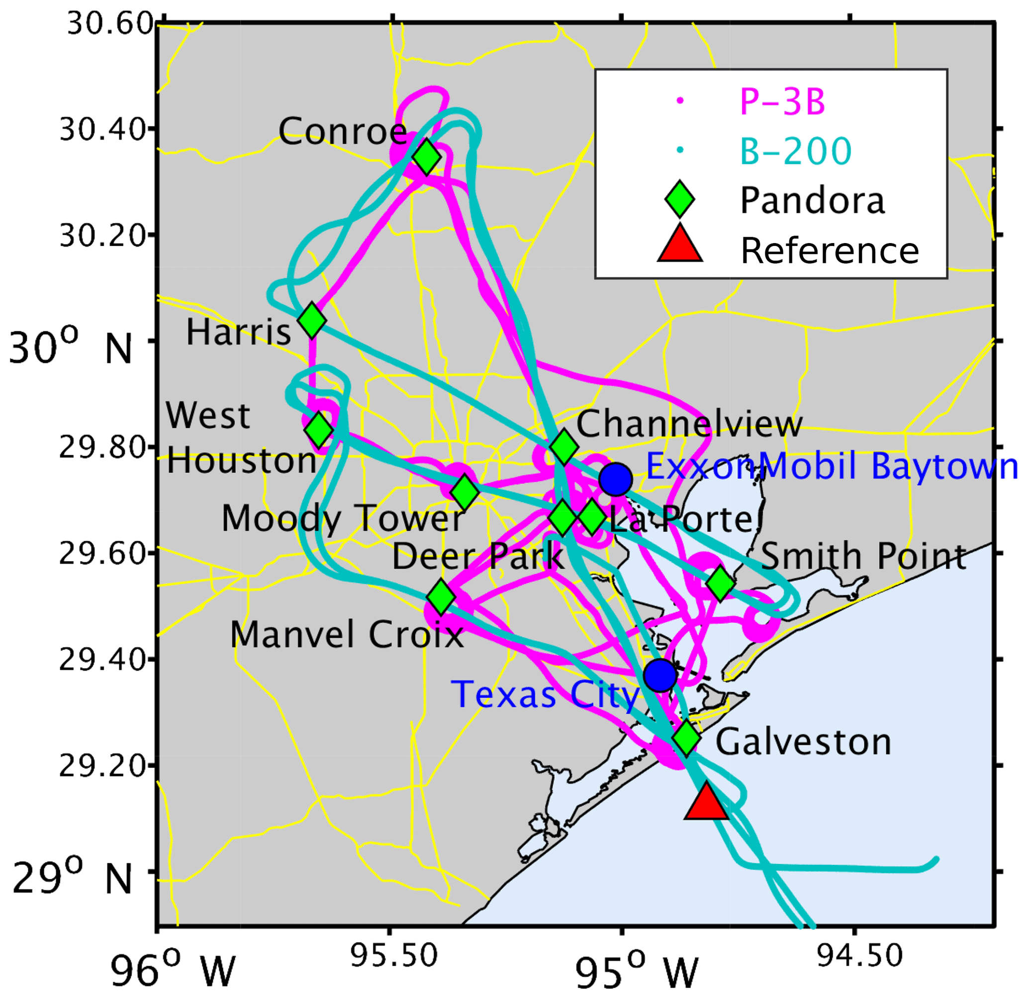
https://www.atmos-meas-tech.net/11/5941/2018/amt-11-5941-2018-f01

Figure 1Map of Houston area showing sample flight tracks for the King Air B-200 (GCAS) and the P-3B aircraft on 6 September 2013, and ground sites where Pandora spectrometers were located. Major roads are shown in yellow. ExxonMobil Baytown and Texas City are large petrochemical and petroleum refinery complexes. The Baytown complex lies near the entrance to the main part of the Houston Ship Channel industrial area, which ends 6.5 km to the east of the downtown. The red triangle shows the location of the observations used to calculate the GCAS reference spectra.

Download

3.2 Pandora observations

Total column observations of NO₂ were made from 15 ground-based Pandora spectrometers viewing in direct-sun (DS) mode (Herman et al., 2009) at 11 sites during the DISCOVER-AQ Texas campaign. GCAS overflew 14 of these spectrometers at 10 sites, which are summarized in Table 2. Pandora NO₂ is determined at a temporal resolution of 90 s using the ratio of direct-sun spectra to a reference spectrum derived by a top-of-the-atmosphere Langley extrapolation using spectra collected on a clear day with low NO₂ (Herman et al., 2009). Spectra are fit from 400 to 440 nm with NO₂ cross sections interpolated to 264 K (Vandaele et al., 1998) and O₃ at 225 K (Brion et al., 1993). At solar zenith angles (SZAs) less than 80^∘, the observed DS slant column is converted to vertical total column using a simple geometric air mass factor (Herman et al., 2009). Pandora DS NO₂ measurements have a nominal precision of 2.7×10¹⁴ molecules cm⁻² and accuracy of 2.7×10¹⁵ molecules cm⁻². Pandora observations with fitting root mean square <0.005 and relative error <10 % are included in this study, to exclude possible cloud-contaminated measurements.

Table 1Summary of GCAS flights during DISCOVER-AQ Texas 2013. Times are local time (LT: UTC − 5 h). Days with P-3B aircraft flights are denoted by an X in the rightmost column.

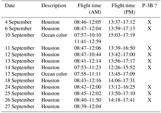
Download Print Version | Download XLSX

Table 2DISCOVER-AQ sites with Pandora spectrometers overflown by GCAS. The Pandora ID is a identification number given to each individual Pandora instrument. Asterisks indicate Pandoras used for MAX-DOAS measurements; all other Pandoras were used solely for direct-sun (DS) measurements. The mean GCAS overpass time of Pandora sites is 10:07 LT (earliest: 08:18 LT; latest: 11:51 LT) for morning flights and 15:25 LT (earliest: 12:51 LT; latest: 17:12 LT) for afternoon flights.

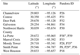
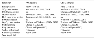
Download Print Version | Download XLSX

Vandaele et al. (1998)Vandaele et al. (1998)Chance and Orphal (2011)Brion et al. (1993)Brion et al. (1993)Rothman et al. (2013)Wilmouth et al. (1999)Thalman and Volkamer (2013)Thalman and Volkamer (2013)Chance et al. (2005)Chance et al. (2005)Chance and Spurr (1997)Chance and Spurr (1997)

Table 3Fitting details and fitted parameters used in GCAS trace gas retrievals. “n/a” means not applicable.

Download Print Version | Download XLSX

Pandoras also operated in multi-axis sky-scanning mode (MAX-DOAS) measuring lower-tropospheric NO₂ distribution and tropospheric columns at the La Porte, Moody Tower and Smith Point sites. Pandora head sensors sequentially pointed at 1, 2, 3, 4, 6, 8, 10, 15, 20, 30, 40 and 90^∘ elevation angles from the horizon with a field of view of 1.6^∘. Azimuth angles were chosen to ensure an unobstructed view down to the horizon and were 320^∘ from north at La Porte, 45^∘ at Moody Tower and 270^∘ at Smith Point. Differential slant column densities of NO₂ and O₂−O₂ within a single scan were calculated using a zenith sky reference spectrum. A temperature-dependent NO₂ absorption cross section (linear and constant terms) and Ring, H₂O and O₂−O₂ cross sections (see Table 3 for references) were used in the MAX-DOAS fitting window 425–490 nm. The profile inversion was performed using the maximum a posteriori optimal estimation method (Rodgers, 2000) with aerosol and gas weighting functions calculated using the Vector Linearized Discrete Ordinate Radiative Transfer (VLIDORT) model (Spurr, 2008). Tropospheric columns were also estimated using a geometrical approach using NO₂ and O₂−O₂ columns derived from 15^∘ elevation angle measurements when inversions failed.

The Pandora dataset contains observations from two Pandora instruments placed at the Moody Tower site at the University of Houston, 70 m above the surface. We correct for the column in the bottom 70 m of the atmosphere using in situ observations at the base and top of the towers collected every 5 min by the University of Houston following Nowlan et al. (2016). The in situ measurements indicated that NO₂ within these altitudes was usually well mixed at the overpasses. This correction varies in magnitude from 0.3×10¹⁵ to 3.7×10¹⁵ molecules cm⁻² for different GCAS overpasses.

3.3 P-3B aircraft observations

The P-3B aircraft carried a suite of in situ instruments in order to profile the atmosphere during the campaign. Profiles were collected during aircraft spirals near eight DISCOVER-AQ ground sites, with each site typically overflown two or three times each day. Depending on the site and flight, the aircraft typically flew between a lowermost altitude of 0–300 m and an uppermost altitude of 3.5–5 km. The typical radius of a spiral was 4–5 km.

The National Center for Atmospheric Research's (NCAR) chemiluminescence instrument (P-CL) (Ridley and Grahek, 1990) measured in situ NO₂ concentrations from the P-3B. P-CL observations of NO₂ have uncertainties of 0.02 ppbv in precision and 10 % in accuracy.

The NCAR Differential Frequency Generation Absorption Spectrometer (DFGAS) (Weibring et al., 2006, 2007) measured in situ CH₂O concentrations from the P-3B. The DFGAS instrument collects data with a temporal resolution of 1 s, with a 15 s background zero-air addition period every 60 to 120 s. This addition captures and removes both inlet/sample cell CH₂O outgassing and optical noise. For a typical spiral, the temporal resolution translates to a vertical resolution of approximately 5 m. The 1 s measurements have a precision of ∼0.08 ppbv (upper limit) and an estimated accuracy of 4 % at the 1σ level.

3.4 Model simulations

This study uses model-simulated trace gas profiles for radiative transfer calculations in order to determine vertical column densities from observed slant column densities. Tropospheric simulations are performed with the Environmental Protection Agency's (EPA) Community Multiscale Air Quality (CMAQ) version 5.0.2 modeling system (Byun and Schere, 2006) over the campaign domain at a spatial resolution of 4×4 km² and a temporal resolution of 20 min. The model has 45 vertical levels from the surface to 50 hPa. The model's vertical resolution ranges from 22 m at the surface to ∼200 m at an altitude of 2 km, further increasing to ∼650 m by the aircraft flight altitude. CMAQ simulations are driven by offline meteorology from the Advanced Research Weather and Forecasting (WRF-ARW) model (Skamarock et al., 2008) via the Meteorology-Chemistry Interface Processor (MCIP) (Otte and Pleim, 2010). Loughner and Follette-Cook (2015) describe the CMAQ and WRF modeling approach used for the DISCOVER-AQ Texas campaign in detail.

Stratospheric NO₂ profiles used in the study are estimated using the PRATMO chemical box model (McLinden et al., 2000; Prather, 1992) from simulated profiles provided as a function of month, solar zenith angle and latitude. Stratospheric ozone profiles are from the September 2013 monthly climatology derived at $1^{\circ} \times 1^{\circ}$ from the OMI ozone profile product (Liu et al., 2010) up to 0.3 hPa.

4 GCAS trace gas retrievals

The GCAS vertical column density retrieval uses a two-step approach. First, we derive the slant column density (SCD) by directly fitting a modeled spectrum to the observed spectrum, starting from a reference spectrum derived from observations over an unpolluted area. Second, we convert SCD to a vertical column density (VCD) using an AMF that represents the path of light through the atmosphere based on the viewing geometry and radiative transfer calculations.

The GCAS trace gas retrieval algorithms used in this paper are derived from the Smithsonian Astrophysical Observatory (SAO) trace gas algorithms originally developed for Global Ozone Monitoring Experiment (GOME), and since applied to GOME-2, SCIAMACHY, OMI, OMPS and GeoTASO for a range of trace gases (Chance, 1998; Chance et al., 2000; Chan Miller et al., 2014; González Abad et al., 2015, 2016; Nowlan et al., 2011, 2016; Sioris et al., 2004; Wang et al., 2014). These algorithms are also the basis for the TEMPO trace gas retrieval algorithms. A separate slant column trace gas product at 350 m × 1000 m was provided by the GCAS instrument team at NASA GSFC to the DISCOVER-AQ data archive shortly after the campaign using the publicly available QDOAS spectral fitting package (http://uv-vis.aeronomie.be/software/QDOAS/, last access: 23 October 2018) and preliminary calibrated spectra. This product is not examined in the current study.

Nowlan et al. (2016) compared preliminary SAO GCAS NO₂ slant columns with GeoTASO slant columns within 10 min and 500 m from four coincident flights during the DISCOVER-AQ Texas campaign (13, 14, 18 and 24 September) at a resolution of 250 m × 500 m. Overall, slant columns agreed well (r=0.81, N=77 320), with GCAS lower than GeoTASO by ∼6 %. The current GCAS retrieval algorithm used in this study is similar to the previous algorithm, but the slant column retrieval uses a separate reference spectrum for each cross-track position and a cross-track dependent instrument line shape, so that the results no longer require a cross-track bias correction. The new NO₂ and CH₂O products also include improved georegistration.

4.1 Spectral calibration

We perform spectral fitting to derive slant columns using radiometrically calibrated spectra (Level 1B), which are geolocated and derived from raw (Level 0) data using characterization data collected in the laboratory before the campaign, as described in detail by Kowalewski and Janz (2014). The first-guess wavelength calibration was determined from spectra collected in the laboratory using mercury–argon, cadmium, neon and krypton discharge lamps as sources. The pre-flight slit function shape and width as functions of cross-track position, wavelength and temperature were also determined using a tunable laser with an integrating sphere. These laboratory tests indicated the instrument's spectral shift is ∼0.004 nm and the change in the slit function's full width at half maximum (FWHM) is less than 0.0013 nm within the instrument's thermal stability range of ±0.25 ^∘C and nominal operating temperature of 20 ^∘C. Pressure changes within the instrument may also shift the wavelength calibration through changes in the index of refraction (Kuhlmann et al., 2016). These changes are minimized in GCAS and are primarily due to changes in ambient temperature, as the instrument is backfilled with gaseous nitrogen and sealed prior to aircraft integration to mitigate moisture. The impact of wavelength shifts on retrievals is further minimized through simultaneous fitting of a wavelength shift for each observation as described in Sect. 4.2.3.

We further refine the instrument spectral registration and slit function calibration using spectra collected during the Texas flights, following our calibration approach previously applied to GOME, GOME-2, OCO-2, ACAM and GeoTASO (Cai et al., 2012; K. Sun et al., 2017 a, b; Liu et al., 2015 b, 2005; Nowlan et al., 2016). As a first step in the spectral fitting, we simultaneously derive a wavelength dispersion and slit function shape by fitting a reference spectrum to a high-spectral-resolution solar atlas (Chance and Kurucz, 2010). This is similar to the approach employed in our satellite retrievals, but, as the airborne nadir reference spectrum contains atmospheric features (which are not present in a satellite-observed exo-atmospheric reference), we also simultaneously fit preliminary amounts of the atmospheric molecular absorbers listed in Table 3 and the Ring effect (rotational Raman scattering) to account for these spectral features (Liu et al., 2015 b; Nowlan et al., 2016).

We determine a separate wavelength dispersion and slit function shape for each of the 21 cross-track positions. The wavelength dispersion is determined by fitting the coefficients in a fifth-order (NO₂) or seventh-order (CH₂O) polynomial that represents the wavelength as a function of detector pixel. For NO₂, we model the slit function using an asymmetric super-Gaussian (Beirle et al., 2017). For CH₂O, we fit parameters describing the shape and width of an asymmetric Gaussian (Cai et al., 2012; Nowlan et al., 2016). While the super-Gaussian works well for NO₂, it results in a very small increase (∼5 %) in fitting residuals for CH₂O over an asymmetric Gaussian, possibly due to the presence of a double shoulder to one side of the slit function shape, as measured in the laboratory at wavelengths less than 380 nm (Kowalewski and Janz, 2014).

The retrieved slit function in the NO₂ fitting window is nearly symmetric and very similar in width to the FWHM = 0.58 nm (Kowalewski and Janz, 2014) measured in the laboratory. Using in-flight data, the retrieved FWHM is 0.57 nm at the nadir center position, expanding to 0.58 nm at the edges of the swath. The retrieved slit width in the CH₂O fitting window changes in a similar way but is larger at the edges (0.57 nm at swath center, growing to 0.60 nm at the leftmost cross-track position (no. 1) and to 0.63 nm at the rightmost cross-track position (no. 21)). We estimate the uncertainty in the slit width is ∼0.01 nm, primarily due to temperature fluctuations during flight. In-flight data show the center detector pixel-to-wavelength registration for both the NO₂ and CH₂O fitting windows varies nearly linearly as a function of swath cross-track position across the left-hand side of the swath, varying by ∼0.1 nm between cross-track positions 1 and 11, but remains approximately constant from positions 11 to 21. The retrieved wavelength calibration is stable to ∼0.002 nm after the instrument has thermally stabilized during flight.

4.2 Slant column retrieval

4.2.1 Spectral fitting

We determine NO₂ and CH₂O slant columns using least-squares minimization to directly fit a modeled radiance spectrum F(x,b) to our observed radiance spectrum. The modeled spectrum is a function of pre-determined model parameters b and the retrieved state vector x. The modeled spectrum is represented by

\begin{array}{l} F (λ) = & ([x_{a} I_{0} (λ) + b_{u} (λ) x_{u} + b_{r} (λ) x_{r}] e^{- \sum_{i} b_{i} (λ) x_{i}}) \\ (1) & \sum_{j} {(λ - \overline{λ})}^{j} x_{j}^{SC} + \sum_{k} (λ - \overline{λ})^{k} x_{k}^{BL} . \end{array}

In this equation, I₀ is a reference spectrum determined from clean nadir observations, scaled by a retrieved intensity parameter x_a (which represents reflectivity factors such as surface albedo or clouds). The derivation of the reference is discussed in Sect. 4.2.2. The term b_u(λ) describes a correction for spectral undersampling (Chance et al., 2005), while b_r(λ) represents the effects of rotational Raman scattering (Chance and Spurr, 1997). The retrieved differential slant columns are represented by x_i. These differential slant columns are the differences between the slant columns in the nadir observation of interest and the slant columns in the reference spectrum. Their absorption cross sections, as listed in Table 3, convolved with the instrument line shape and corrected for the “I₀ effect” (Aliwell et al., 2002), are included as b_i(λ). In addition, the retrieval also determines scaling (of order j) and baseline (of order k) wavelength-dependent polynomial coefficients (x^SC and x^BL) that represent low-frequency wavelength-dependent effects from surface reflectivity, molecular scattering, aerosols and instrument artifacts.

4.2.2 Reference spectrum

Each trace gas retrieval uses a reference spectrum determined from nadir observations over a clean area. We determine a mean reference spectrum for each of the 21 cross-track positions by averaging 40 spectra at 250 m × 500 m resolution for each cross-track position from a cloud-free and clean area over the Gulf of Mexico during the 6 September afternoon flight. This location and date were chosen after CMAQ simulations and preliminary retrievals of NO₂ and CH₂O predicted relatively low columns of those trace gases. In addition, we found that the use of a reference collected before the instrument was thermally stable (within the first ∼40 min of a flight) resulted in cross-track biases in the CH₂O retrieval. As observations over the relatively clean Gulf are often collected in the period soon after takeoff, this constraint limited the availability of a suitable reference to a reference spectrum taken late in the flight, close to landing, and with a relatively high solar zenith angle (58^∘).

We use a single reference spectrum at each cross-track position for the entire campaign, instead of a daily or higher-frequency reference, to ensure that all days during the campaign have the same background correction applied for the reference spectrum. Due to the use of a nadir reference, the retrieved differential slant columns must be corrected by the reference background column derived from the model to produce an effective tropospheric column (discussed in further detail in Sect. 4.3). We find that the use of a single reference for the campaign removes day-to-day relative background biases in the GCAS column that can result from uncertainties in daily modeled columns and improves the daily consistency of background CH₂O in the in situ P-3B CH₂O comparison discussed later in Sect. 6.1. The use of a single versus daily reference spectrum has little effect on the NO₂ validation.

4.2.3 NO₂ and CH₂O fitting

The NO₂ and CH₂O slant column density retrievals use the fitting parameters summarized in Table 3. NO₂ is fit at wavelengths 420–465 nm with an NO₂ absorption cross section at 294 K. The NO₂ retrieval also simultaneously fits O₃ at two temperatures, as well as H₂O vapor and O₂−O₂, which all have spectral absorption features in the NO₂ wavelength fitting window. The CH₂O retrieval is performed at 328.5–356.5 nm and simultaneously fits NO₂, O₃, BrO and O₂−O₂. Both retrievals also fit the undersampling correction, Ring spectrum, a fifth-order scaling polynomial and a fourth-order baseline polynomial. Each retrieval also determines a wavelength shift that represents the relative difference in the detector pixel to wavelength registration between the radiance and reference spectra.

4.3 Conversion to vertical column

For air quality applications, we are interested in the vertical column density, V, of the trace gas (NO₂ or CH₂O) in the troposphere. The vertical column density can be derived from the slant column density, S, using an air mass factor, A, which describes the mean light path through the atmosphere, by

\begin{matrix} (2) & V = \frac{S}{A} . \end{matrix}

In practice, the retrieval algorithm determines a differential slant column ΔS, which is the difference between the slant column S of the absorber in the spectrum of interest and the slant column S_R in the reference spectrum. Each of these slant columns is the sum of the slant column of absorber in the light path above (↑) and below (↓) the aircraft, so that

\begin{matrix} (3) & Δ S = (S^{↓} + S^{↑}) - (S_{R}^{↓} + S_{R}^{↑}) . \end{matrix}

In terms of the air mass factor and vertical column, the vertical column below the aircraft can then be expressed as

\begin{matrix} (4) & V^{↓} = \frac{Δ S - V^{↑} A^{↑} + V_{R}^{↓} A_{R}^{↓} + V_{R}^{↑} A_{R}^{↑}}{A^{↓}}, \end{matrix}

where the vertical columns V^↑, $V_{R}^{↓}$ and $V_{R}^{↑}$ are typically determined from a model. Because the flight altitude of 9 km is well above the majority of tropospheric NO₂ and CH₂O, we refer to V^↓ and V^↑ as the tropospheric and stratospheric trace gas columns. NO₂ above the aircraft is dominated by stratospheric NO₂, varies primarily by time of day and ranges within $V^{↑} = 2.3$ –3.8×10¹⁵ molecules cm⁻². CH₂O in the model is more variable, with the early part of the campaign (4 to 18 September) seeing levels of $V^{↑} = 2$ –25×10¹⁴ molecules cm⁻² and the latter part seeing levels of $V^{↑} = 1$ –3×10¹⁴ molecules cm⁻². For our chosen reference location, the modeled vertical columns below the aircraft are $V_{R}^{↓} = 2.0 \times 10^{15}$ molecules cm⁻² for NO₂ and $V_{R}^{↓} = 7.5 \times 10^{15}$ molecules cm⁻² for CH₂O. The modeled vertical columns above the aircraft at the reference location are $V_{R}^{↑} = 3.6 \times 10^{15}$ molecules cm⁻² for NO₂ and $V_{R}^{↑} = 7.9 \times 10^{14}$ molecules cm⁻² for CH₂O.

4.3.1 Air mass factor calculation

We calculate the air mass factors on a scene-by-scene basis using the formulation of Palmer et al. (2001) and Martin et al. (2002) with the VLIDORT radiative transfer model (Spurr, 2008, 2006). In this approach, the radiative transfer model provides scattering weights w as a function of altitude z. The scattering weights describe the sensitivity of the measurement to the different altitude layers and are a function of the viewing geometry, ozone profile, aerosol and molecular scattering, and surface reflectance. These can be used with shape factor s, which is the normalized partial column n of the trace gas at each altitude layer:

\begin{matrix} (5) & s (z) = \frac{n (z)}{\int_{z} n (z) d z} . \end{matrix}

The AMF is defined as

\begin{matrix} (6) & A = \int_{z} w (z) s (z) d z . \end{matrix}

The air mass factor below the aircraft A^↓ is calculated from the surface z₀ to the aircraft altitude z_ac as

\begin{matrix} (7) & A^{↓} = \int_{z_{0}}^{z_{ac}} w (z) s (z) d z, \end{matrix}

while the air mass factor above the aircraft A^↑ is determined from the aircraft altitude to the top of the atmosphere at z_TOA, with

\begin{matrix} (8) & A^{↑} = \int_{z_{ac}}^{z_{TOA}} w (z) s (z) d z . \end{matrix}

4.3.2 Radiative transfer calculations

We use the radiative transfer algorithm to determine scattering weights in 56 vertical layers. These include the 45 CMAQ layers up to ∼19 km and 11 additional layers to 0.3 hPa. We use the MODIS BRDF (bidirectional reflectance distribution functions) gap-filled MCD43GF V005 Band 3 product (Q. Sun et al., 2017; Schaaf et al., 2002) to represent surface reflectance in the VLIDORT model. This BRDF product is provided at a spatial resolution of 30 arcsec (∼ 0.80 km in longitude by 0.92 km in latitude over Houston) every 8 days, based on 16 days of MODIS measurements. The MODIS Band 3 product is derived at 470 nm. While this is close to the NO₂ fitting window, there currently exists no BRDF climatology at shorter wavelengths. We determine effective BRDFs at 442 nm (NO₂) and 342 nm (CH₂O) by scaling the BRDF functions by the ratio of the ${0.5}^{\circ} \times {0.5}^{\circ}$ monthly OMI Earth Surface Reflectance Climatology product (OMLER) (Kleipool et al., 2008) at either 442 or 342 nm to its value at 470 nm. These results are typically within 2 %–3 % of the results derived using a black-sky/white-sky approach to estimate surface reflectance (McLinden et al., 2014).

Figure 2 shows profiles for (1) a sample polluted observation at the Moody Tower site in downtown Houston and (2) the reference spectrum. For the AMF calculation, the shape factors are derived from the model profiles shown in Fig. 2a and c and then applied to the corresponding scattering weights. Differences in the scattering weights of the reference and Moody Tower observations at higher altitudes are mainly driven by differences in the solar zenith angles. The smaller CH₂O scattering weights near the surface relative to those of NO₂ indicate the relatively lower sensitivity of the observations to near-surface CH₂O. This is due primarily to the wavelength dependency of the AMF, as stronger Rayleigh scattering and ozone absorption at shorter wavelengths decreases the measurement sensitivity to lower altitudes. The AMF is calculated scene by scene for each nadir observation. The reference spectrum AMFs at the swath center are $A_{R}^{↓} = 1.65$ and $A_{R}^{↑} = 1.92$ for NO₂ and $A_{R}^{↓} = 2.03$ and $A_{R}^{↑} = 2.49$ for CH₂O.

https://www.atmos-meas-tech.net/11/5941/2018/amt-11-5941-2018-f02

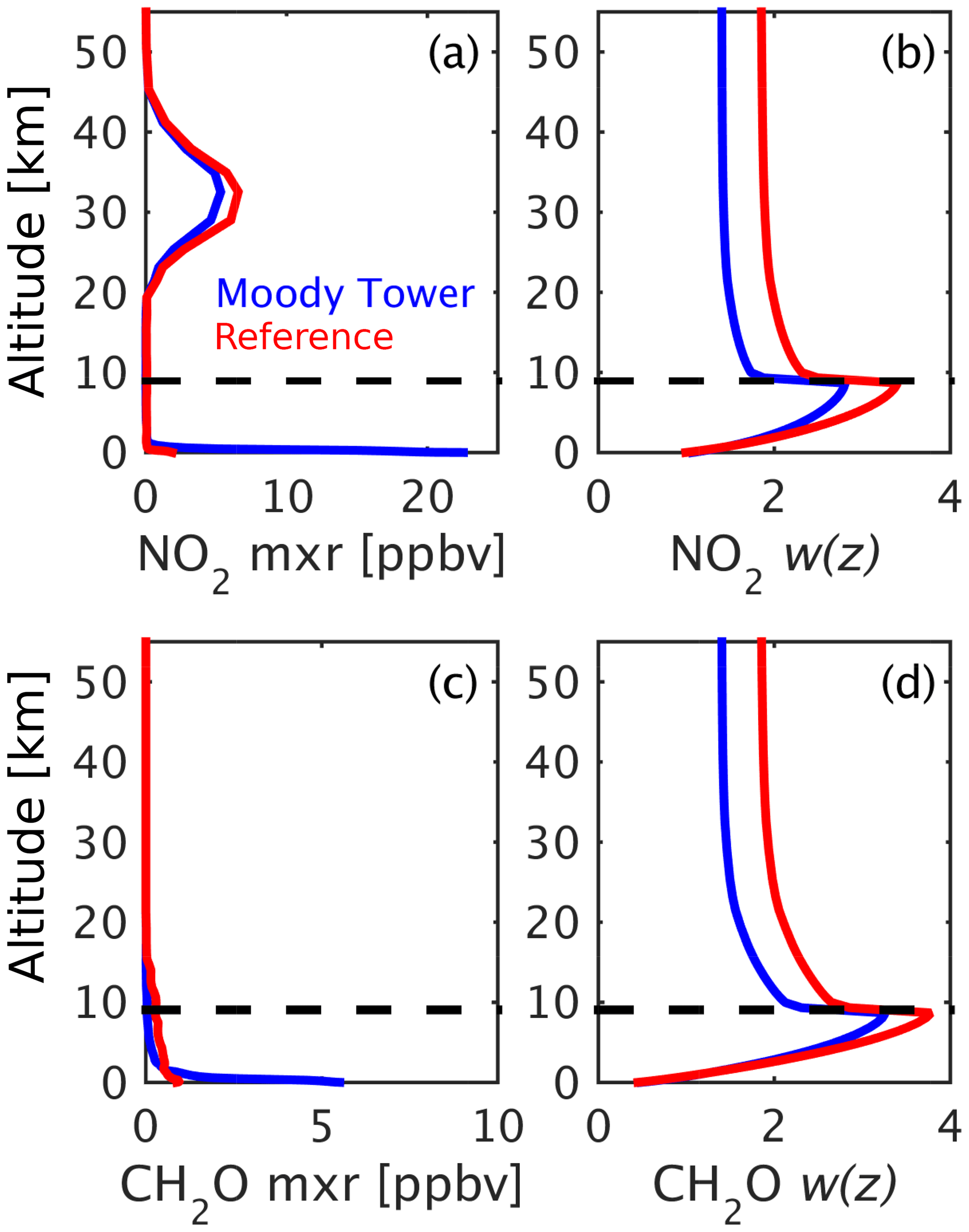
Figure 2Sample mixing ratio (mxr) and scattering weight (w(z)) profiles used in the GCAS AMF calculations. The reference spectrum profiles are taken from the 6 September afternoon flight over the Gulf of Mexico at an average location of 29.126^∘ N, 94.818^∘ W at 17:04 LT (local time: UTC time − 5 h) with SZA = 58.0^∘and VZA = 10.5^∘. The profiles at the Moody Tower site in downtown Houston are from the 25 September morning flight at 10:56 LT with SZA = 45.0^∘and VZA = 10.7^∘. The estimated surface reflectivities at 442 nm (NO₂) and 342 nm (CH₂O) are 0.04 and 0.05 at the reference location and are both 0.07 at Moody Tower. The dashed black line indicates the aircraft flight altitude.

Download

4.4 Cloud flagging

Only cloud-free measurements are used in this study, and the radiative transfer calculations assume cloud-free conditions. Unlike the case of satellite observations with footprints on the order of tens of square kilometers, GCAS observations are of sufficiently high spatial resolution that cloudy pixels can be discarded without loss of a significant amount of data. We flag as cloudy any pixel that has a mean radiance in the NO₂ fitting window over a threshold of 2×10¹³ $photons {cm}^{- 2} {nm}^{- 1} s^{- 1} {sr}^{- 1}$ , which is typically only exceeded in the case of a bright cloud. The Ring scattering parameter retrieved simultaneously with NO₂ and a color index (the radiance ratio at wavelengths 320 to 440 nm) are also used to flag less bright pixels where clouds likely occur (Wagner et al., 2014).

4.5 Trace gas uncertainties

Uncertainties in the vertical column density result from uncertainties in (1) the slant column fitting; (2) the air mass factor calculation; and (3) the modeled reference and stratospheric columns needed for determining the vertical column below the aircraft using Eq. (4).

4.5.1 Slant column uncertainties

The slant column fitting uncertainty on a single observation is dominated by the random noise in the spectrum. Over a typical day, the mean fitting uncertainty in an NO₂ differential slant column at 250 m × 500 m resolution is 1.3×10¹⁵ molecules cm⁻², including all solar zenith angles in the morning and afternoon flights. The typical fitting uncertainty in a CH₂O differential slant column is 2.5×10¹⁶ molecules cm⁻². After AMFs are applied, typical mean vertical column precisions are 1×10¹⁵ molecules cm⁻² for NO₂ and 1.9×10¹⁶ molecules cm⁻² for CH₂O. The precision requirements of the TEMPO instrument are 1×10¹⁵ molecules cm⁻² for NO₂ and 1×10¹⁶ molecules cm⁻² for CH₂O (Zoogman et al., 2017). (Note that the signal-to-noise ratio is higher at CH₂O wavelengths relative to that at NO₂ wavelengths for TEMPO, which is the opposite of GCAS.) CH₂O in particular is noisy at the provided GCAS spatial resolution of 250 m × 500 m, with enhanced CH₂O columns often on the order of the retrieval precision. GCAS CH₂O must be spatially averaged to meet the TEMPO precision requirement and to improve the detection limit in order to observe polluted columns over Houston. As a result, later in this paper we present CH₂O maps at 1 km² resolution, with an effective precision on the order of 7×10¹⁵ molecules cm⁻². It should be noted that, even at precisions of 1×10¹⁶ molecules cm⁻², CH₂O columns from satellite instruments like OMI typically must be temporally averaged to resolve local CH₂O features (Marais et al., 2014; Zhu et al., 2014).

Additional errors in NO₂ slant column retrievals can also result from the use of an NO₂ cross section at a single temperature (Boersma et al., 2004). The profile-weighted effective temperature of NO₂ during the Houston campaign in polluted observations was typically within a few degrees of the 294 K cross-section temperature, resulting in an expected bias within 1 %–2 % in the tropospheric slant column. The stratospheric slant column may be biased by ∼15 % due to its colder temperature, but the influence of this uncertainty is minimized by the use of a nadir reference spectrum, resulting in a possible systematic bias on the order of 4×10¹⁴ molecules cm⁻² (an uncertainty of 1 %–2 % for polluted pixels). Uncertainties in the laboratory cross sections introduce additional uncertainties in the slant columns of 2 % for NO₂ (Boersma et al., 2004) and 5 % for CH₂O (Chance and Orphal, 2011). Uncertainties in the differential slant columns due to uncertainties in the spectral calibration are $\sim 5 \times 10^{13}$ molecules cm⁻² for NO₂ and $\sim 2 \times 10^{15}$ molecules cm⁻² for CH₂O.

4.5.2 Air mass factor uncertainties

The air mass factor uncertainties in cloud-free satellite observations are typically dominated by uncertainties in the surface albedo, trace gas profile shape and aerosols (Boersma et al., 2004). A recent study by Lorente et al. (2017) found an average AMF structural uncertainty of 42 % in polluted observations and 31 % in unpolluted regions when different retrieval groups used different inputs to NO₂ AMF calculations; the most significant impacts overall were from differences in surface albedo, cloud parameters and trace gas profile inputs.

MODIS BRDF comparisons with aircraft observations of the surface indicate an uncertainty in the MODIS BRDF product of 20 % for both accuracy and precision (Román et al., 2011) at GCAS spatial resolutions. We estimate the impact of those uncertainties from the MODIS surface BRDF on our individual AMFs to be 10 % for polluted observations and 5 % for clean observations. Y. Wang et al. (2010) showed that the use of the Lambertian approximation in the derivation of the MODIS products may result in surface reflectance underestimation of 0.008 by MODIS in the green bands. This surface bias on average could cause the GCAS AMF to be underestimated (and the resulting trace gas column to be overestimated) by ∼10 %.

The radiative effects of aerosols are not typically included in operational satellite retrieval trace gas AMFs, except as an implicit component of the cloud fraction, and we have not included aerosols in the current study. In reality, the presence of aerosols can increase or decrease the AMF, with effects depending on aerosol type and altitude (Chimot et al., 2016; Kwon et al., 2017; Leitão et al., 2010; Lin et al., 2014; Meier et al., 2017). When scattering aerosols are in the boundary layer, for example, the backscattered light path increases the radiative sensitivity (an enhancement effect), resulting in an increase in the AMF. Ignoring these aerosols in the radiative transfer calculation will cause the retrieved column to be overestimated. When scattering aerosols are aloft, the radiative sensitivity decreases near the surface (a shielding effect), resulting in a decrease in the AMF. Absorbing aerosols aloft or at the altitude of the trace gas can decrease the measurement sensitivity by reducing the number of photons backscattered to the instrument, thereby reducing the AMF. Even when aerosols are considered, assumptions about aerosol optical properties and profiles can cause large uncertainties; Lorente et al. (2017) found different aerosol corrections used by different research groups introduced an average uncertainty of 50 % for polluted satellite observations with high aerosol loading.

Aerosol optical depth (AOD) measured by the HSRL lidar on the B-200 (Sawamura et al., 2017) showed aerosols varying day to day along the flight track and with altitude during the DISCOVER-AQ Texas campaign. The beginning of the campaign saw moderate AOD on the order of 0.2–0.3 (532 nm), often with a smoke plume at altitudes 2–4 km which sometimes merged with aerosols from lower layers later in the day. Observed AODs rose sharply on 14 September, with AODs in excess of 0.7 in some areas. Aerosol loading from 18 September onwards was relatively low (<0.15) and primarily located near the surface, with AOD occasionally reaching 0.25 at some points along the flight track. A full assessment of the effects of aerosols on the AMF is beyond the scope of this paper and the subject of ongoing work, but our simulations with typical AOD profiles from the HSRL lidar show a potential overestimation of the column of 10 %–30 % for individual polluted pixels when scattering aerosols in the planetary boundary layer (PBL) are ignored and a potential 15 % underestimation of the column when the smoke layer aloft is ignored. These results are consistent with Lin et al. (2014), whose satellite biases are typically within ±25 % due to the neglect of aerosols at these AODs.

Nowlan et al. (2016) previously compared mean profile shapes from the P-CL observations and the CMAQ simulations for the eight core ground sites during DISCOVER-AQ Texas; mean differences were typically within 20 % for individual sites. Individual total column observations can vary by >100 % (Nowlan et al., 2016), with differences mostly resulting from the small-scale features of NO₂ plumes, which are difficult to resolve with model resolution. Previous comparisons of DISCOVER-AQ Texas CMAQ CH₂O 1 km simulations with P-3B DFGAS observations showed agreement between the model and observations for most days of the campaign (Fried et al., 2016 b). The average of daily mean biases indicated a low bias of CMAQ relative to DFGAS of $- 0.44 \pm 0.39$ ppbv in the PBL and $- 0.32 \pm 0.40$ ppbv overall ( $- 11.8 \pm 15.7$ %) over all days, excluding 25 September: a unique day characterized by very large CH₂O levels of up to 25 ppbv as measured by the DFGAS instrument on the P-3B in the boundary layer over petrochemical facilities in Houston and up to 33 ppbv downwind over Galveston Bay and Smith Point later in the day due to photochemical processing (Fried et al., 2016 b). From P-3B comparisons discussed later in this paper (Sect. 6.3), we estimate these profile shape uncertainties typically result in uncertainties in the AMF of 10 % for NO₂ and 8 % for CH₂O.

Souri et al. (2018) calculated GCAS NO₂ vertical columns independently for our derived slant columns and found a mean tropospheric AMF over all days of 1.26±0.32. This compares closely with our mean AMF of 1.29 ± 0.27. Their inputs included MODIS BRDF for surface reflectance, GEOS-Chem modeled stratospheric profiles, and an independently run CMAQ simulation whose aerosol fields were used to determine aerosol optical depths for input to the VLIDORT model. The similar AMF from a separate study suggests a low structural uncertainty in AMF calculations using currently available ancillary information.

4.5.3 Modeled column uncertainties

Equation (4) requires the modeled vertical column below the aircraft at the reference spectrum location ( $V_{R}^{↓}$ ) and the modeled vertical columns above the aircraft at the observation location (V^↑) and the reference location ( $V_{R}^{↑}$ ). Systematic uncertainties in the effective slant columns above the aircraft at the observation and the reference may cancel out to some degree, but small uncertainties may still propagate to the final vertical column through the use of different observation and reference times and locations. We estimate an uncertainty of 30 % in the NO₂ stratospheric column, based on PRATMO comparisons with the Optical Spectrograph and InfraRed Imaging System (OSIRIS) limb sounder (Bourassa et al., 2011). We estimate reference location tropospheric vertical column uncertainties of 40 % for NO₂ and 31 % for CH₂O, based on comparisons of the CMAQ model columns with the P-3B-inferred columns of the four cleanest spirals during the campaign at the coastal sites Galveston and Smith Point. An additional uncertainty is added by uncertainty in the reference AMFs, as discussed in the previous section.

4.5.4 Total uncertainties

We estimate total uncertainties by error propagation through Eq. (4). Total uncertainties in cloud-free tropospheric NO₂ columns at 250 m × 500 m resolution range from 30 % to >100 % for clean pixels ( $< 0.5 \times 10^{16}$ molecules cm⁻²), 20 % to 50 % for moderately polluted pixels (0.5–1×10¹⁶ molecules cm⁻²) and 18 % to 30 % for more heavily polluted pixels ( $> 2 \times 10^{16}$ molecules cm⁻²). Total uncertainties in CH₂O columns at this spatial resolution vary from 30 % to >100 % for clean pixels ( $< 1 \times 10^{16}$ molecules cm⁻²), 20 % to 50 % for moderately polluted pixels (1–2×10¹⁶ molecules cm⁻²) and 18 % to 40 % for very polluted pixels ( $> 2 \times 10^{16}$ molecules cm⁻²).

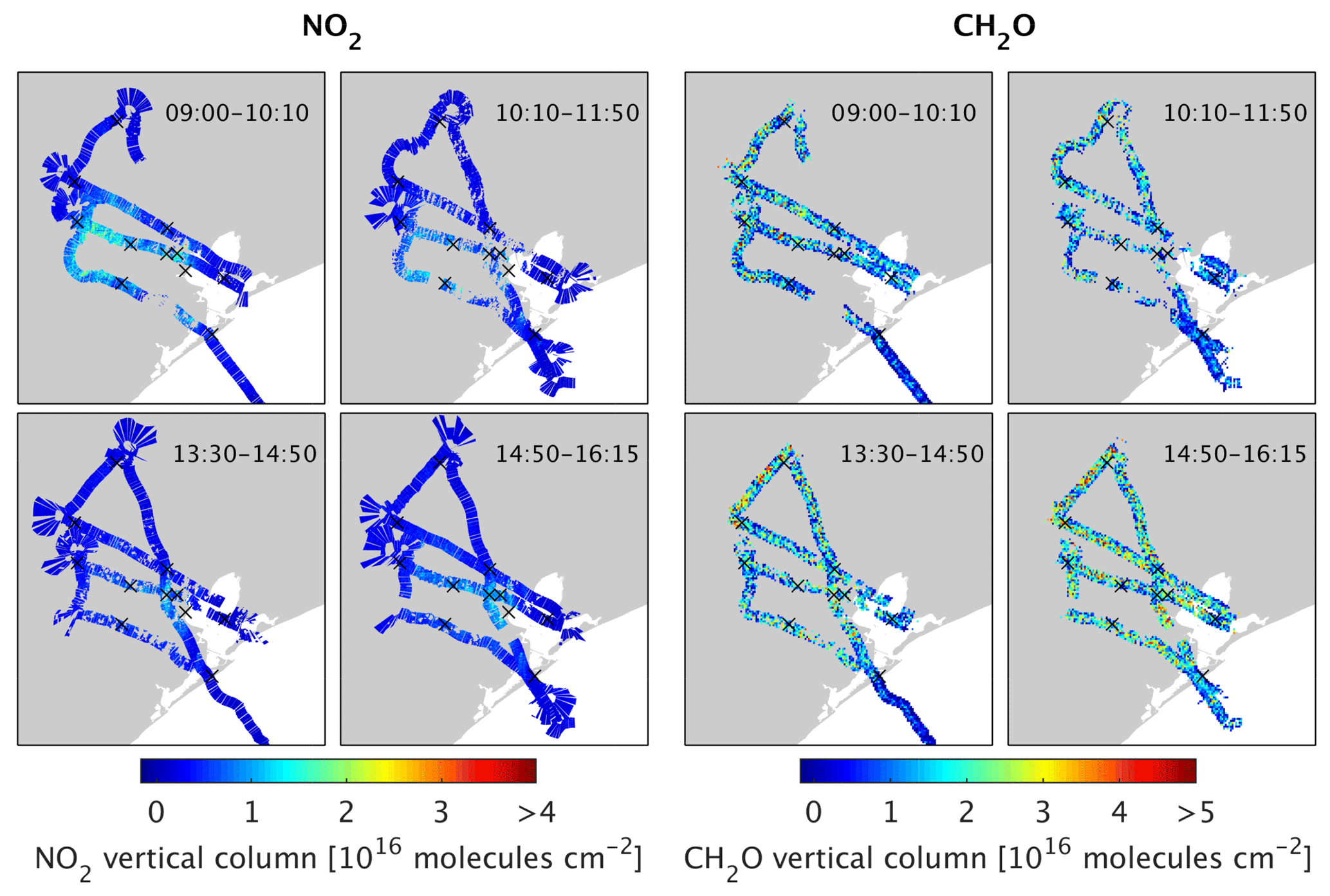
https://www.atmos-meas-tech.net/11/5941/2018/amt-11-5941-2018-f03

Figure 3Tropospheric NO₂ and CH₂O vertical columns measured by GCAS over Houston on 24 September 2013. NO₂ observations are at ∼250 m × 500 m resolution, and CH₂O columns are at $0.01^{\circ} \times 0.01^{\circ}$ (∼1 km²) resolution. Times are local time. Black crosses indicate ground sites.

Download

https://www.atmos-meas-tech.net/11/5941/2018/amt-11-5941-2018-f04

Figure 4Same as Fig. 3 but for 25 September 2013.

Download

5 Vertical column results

Retrieved GCAS columns in the Houston area during the campaign show enhanced NO₂ amounts over central Houston (close to Moody Tower), in the vicinity of the Houston Ship Channel industrial area (Pandora sites Channelview, Deer Park and La Porte) and sometimes along the more suburban flight track to the west of and over Manvel Croix, which is the case for morning overpasses on 6 and 13 September (Nowlan et al., 2016). Individual NO₂ plumes can also often be observed from single industrial sites and stacks. Emissions estimates using GCAS and CMAQ indicate the highest source regions for NO_x are the Houston metropolitan area (145 t day⁻¹), where mobile sources dominate; the Houston Ship Channel region (54 t day⁻¹), where many petrochemical plants are concentrated; and, to a lesser extent, the Texas City area (17 t day⁻¹), which is home to petroleum refining and petrochemical processing facilities (Souri et al., 2018).

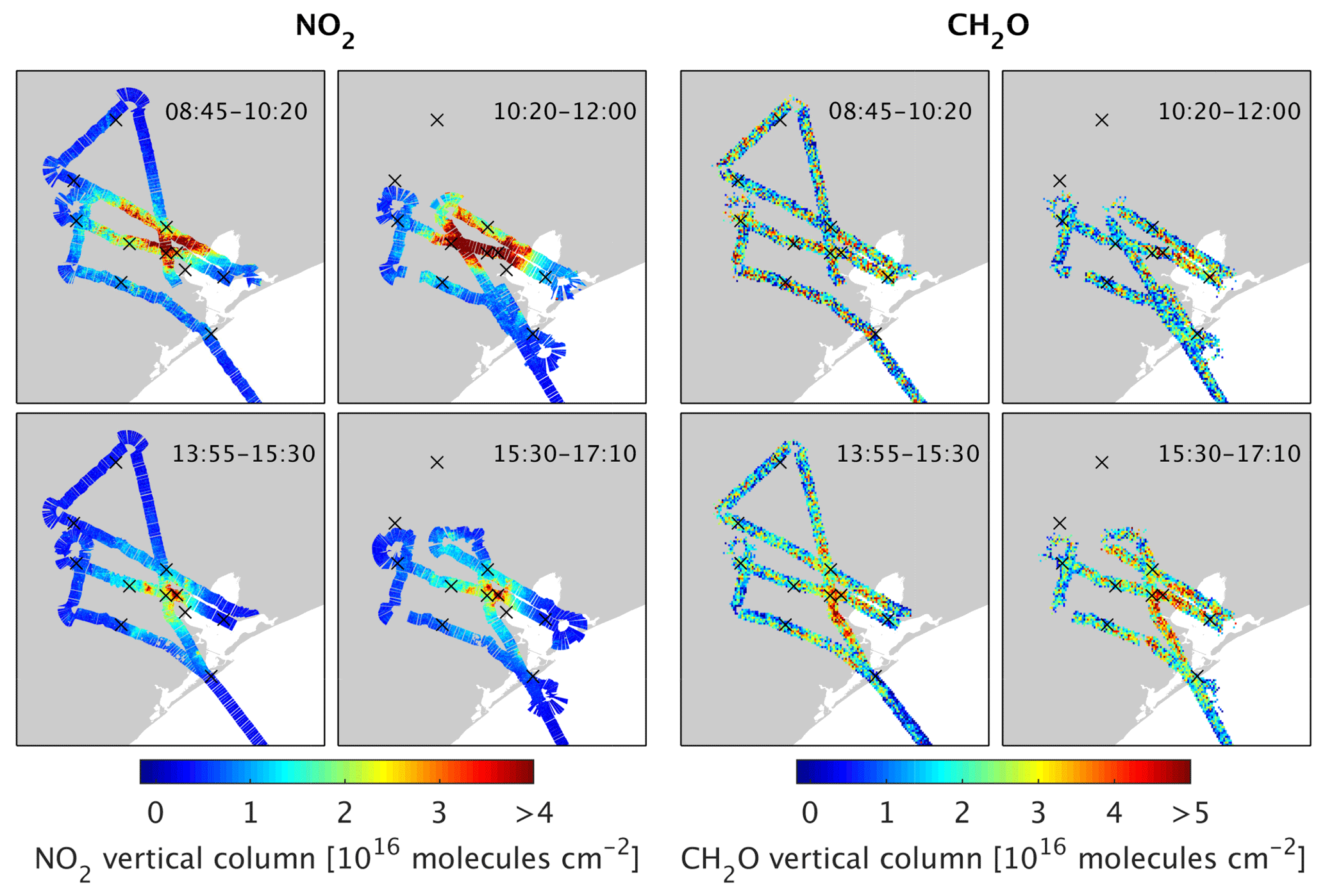
Figures 3 and 4 show examples of retrieved NO₂ and CH₂O tropospheric vertical columns for two consecutive days during the campaign and illustrate both the day-to-day and hourly variabilities observed in NO₂ and CH₂O columns. In general, the largest NO₂ columns are seen in morning flights during all days of the campaign, with the peak columns varying with overpass time and meteorological conditions. The day of 24 September is typical of columns measured during the campaign in terms of magnitude. The 25 September flights show the largest pollution episode of the campaign.

Formaldehyde observations are noisier, but enhanced CH₂O columns are clearly observable on some days when data are spatially averaged. In particular, 4 and 25 September show the largest CH₂O enhancements, with peak values on the order of 5×10¹⁶ molecules cm⁻² at 1 km² resolution. Figure 4 shows the significant enhancement in CH₂O near the Houston Ship Channel industrial area on 25 September. Several other days exhibit enhanced background over land, with the largest values of CH₂O columns on these days to the north of Houston over the Conroe region, potentially from biogenic sources as well as transport of CH₂O and its precursors. These days with large background CH₂O highlight the importance of using the clean reference over the water, where background CH₂O is typically lower than over land.

The month of September 2013 was relatively dry over Houston, and B-200 flights typically occurred on dry days with little cloud cover. Li et al. (2016) and Loughner and Follette-Cook (2015) describe the overall meteorological conditions present during the campaign as well as detailed meteorological conditions on certain days. In the early part of September, the area saw little influence from strong synoptic weather systems, with winds mostly light and northeasterly in the early morning, shifting clockwise to southeasterly in the afternoons and resulting in the transport of clean marine air over Houston. The days of 11–14 September were characterized by winds from the northeast, parallel to the coastline. A cold front passed over Houston with northerly transport on 24 September, while 26 September saw stagnant conditions overnight, followed by a sea breeze.

The 25 September pollution episode has been previously examined in several model and in situ measurement studies (Fried et al., 2016 b; Li et al., 2016; Loughner and Follette-Cook, 2015; Mazzuca et al., 2017; Pan et al., 2017; Souri et al., 2016). This day saw a light morning land breeze which removed pollutants from the Ship Channel to Galveston Bay. A later bay breeze then brought pollutants from the bay back to land. In the mid-morning, the prevailing winds were northwesterly over most of the city, with northeasterly winds observed at the Houston Ship Channel. When combined with the bay breeze, these winds set up a convergence zone, trapping pollutants from the Ship Channel region. In combination with a suspected emissions event (Fried et al., 2016 b; Souri et al., 2018), these meteorological conditions produced very high levels of ozone, NO₂, CH₂O and related species. NO₂ columns on this day are largest in the morning flight, while CH₂O columns are largest in the afternoon. GCAS is likely measuring both directly emitted CH₂O and secondary CH₂O produced from other precursors.

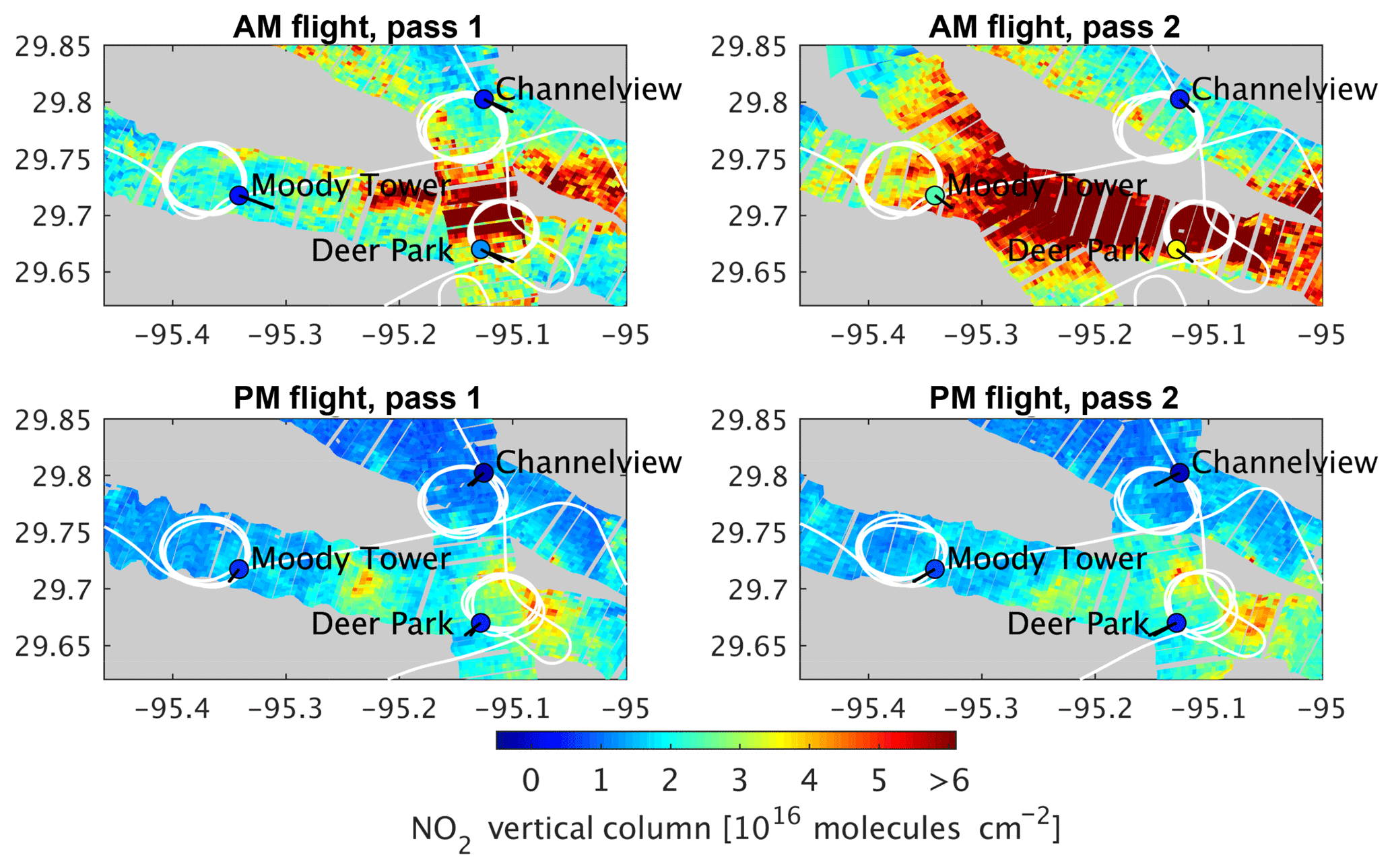
https://www.atmos-meas-tech.net/11/5941/2018/amt-11-5941-2018-f05

Figure 5GCAS tropospheric NO₂ columns measured near DISCOVER-AQ ground sites in the area of downtown Houston on 25 September 2013. P-3B flight tracks are shown in white. Pandora direct-sun NO₂ tropospheric columns (total column NO₂ minus modeled NO₂ above the aircraft) are shown in filled circles. Black lines represent the line of sight of each Pandora intersecting the bottom 2 km of the atmosphere. The largest NO₂ column observed by GCAS on this day was 16×10¹⁶ molecules cm⁻². The NO₂ precision at this resolution is $\sim 1 \times 10^{15}$ molecules cm⁻². Periodic cross-track gaps in the data are due to write-to-disk intervals of the instrument. During these periods, the instrument does not acquire data, thus producing small gaps in coverage.

Download

https://www.atmos-meas-tech.net/11/5941/2018/amt-11-5941-2018-f06

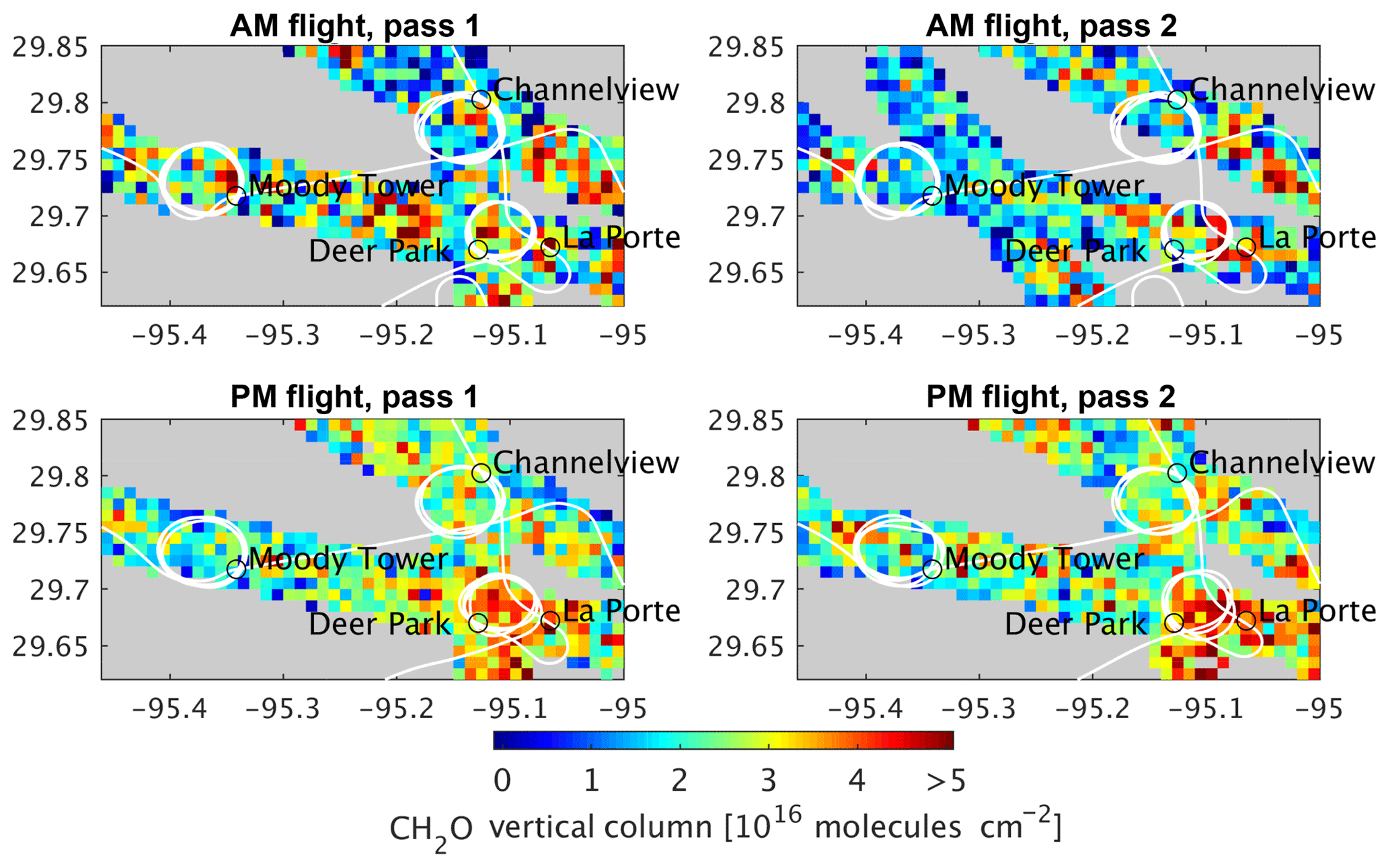
Figure 6GCAS tropospheric CH₂O columns measured near DISCOVER-AQ ground sites in the area of downtown Houston on 25 September 2013. P-3B flight tracks are shown in white. CH₂O columns are spatially averaged on a $0.01^{\circ} \times 0.01^{\circ}$ grid (∼1 km²). The CH₂O precision at this resolution is $\sim 7 \times 10^{15}$ molecules cm⁻².

Download

6 Comparisons with coincident measurements

In this section, we compare GCAS observations from all days with coincident observations from Pandoras and the P-3B aircraft. Figures 5 and 6 show enlarged views of NO₂ and CH₂O observations over the downtown and Ship Channel regions of Houston on 25 September, along with coincident Pandora ground site observations and the P-3B flight track nearest in time. These figures illustrate the typical coverage of P-3B spirals relative to GCAS swaths, as well as the air mass measured in the bottom 2 km of the atmosphere by Pandora DS ground-based instruments.

6.1 P-3B airborne in situ measurements

We compare the retrieved GCAS NO₂ and CH₂O columns with columns derived from in situ observations on the P-3B aircraft. The P-3B profiles are converted into column amounts below the top flight altitude (usually 3.5–5 km) using mixing ratios and pressure/temperature profiles measured on board the P-3B aircraft. Comparisons between GCAS and P-3B columns are shown in Fig. 7.

https://www.atmos-meas-tech.net/11/5941/2018/amt-11-5941-2018-f07

Figure 7Columns derived from in situ measurements of (a) NO₂ from the chemiluminescence instrument and (b) CH₂O from the DFGAS instrument on the P-3B aircraft compared with vertical columns measured by the GCAS instrument, over 9 days during the DISCOVER-AQ Texas campaign. Each GCAS vertical column is the mean of all retrieved cloud-free GCAS columns below the aircraft within 5 km and 1 h of its coincident P-3B spiral center. GCAS air mass factors are determined using modeled CMAQ profiles. The solid line represents the 1 : 1 ratio. The dotted line represents the reduced major axis linear regression. Error bars represent the uncertainty in the GCAS mean column due to retrieval noise from the observations used to calculate a mean column (typically several hundred at 250 m × 500 m resolution); in the case of NO₂, this uncertainty is generally negligible due to low relative error. Column precisions for P-3B observations are approximately 2×10¹³ molecules cm⁻² (NO₂) and 6×10¹³ molecules cm⁻² (CH₂O). Uncertainties from spatial variability and measurement accuracy are discussed in the text.

Download

6.1.1 P-3B and GCAS column preparation

Each P-3B column is calculated by integrating the NO₂ or CH₂O partial columns derived from observed mixing ratios over the altitude of the spiral. The lowest altitude of each P-3B spiral varies by location. At Deer Park, Galveston and West Houston, the mean minimum spiral altitude is ∼20–40 m, while Conroe and Smith Point spirals typically go as low as ∼130 m. At Channelview, Manvel Croix and Moody Tower, the lowest spiral altitude is typically ∼300 m. To determine the NO₂ profile below the lowest P-3B altitude, we estimate the P-3B mixing ratio below the aircraft following Lamsal et al. (2014), by extrapolating the mixing ratio at the lowest aircraft altitude to the surface using the vertical gradient from the CMAQ model at altitudes below the spiral. A large source of error from these extrapolations is the inhomogeneity of the trace gas field, which is particularly strong for NO₂ (see Fig. 5 for example), as the lowest mixing ratio could be measured in or out of an area of high NO₂ and is then extended to the ground. Lamsal et al. (2014) estimated errors in the DISCOVER-AQ Maryland P-3B NO₂ columns of generally less than 20 % from extrapolation of the NO₂ profile below ∼300 m, assuming a factor-of-2 error in the extrapolation. CH₂O DFGAS mixing ratios below the spiral are extrapolated to the ground from the lowest mixing ratio in the bottom 100 m of the spiral, as described by Fried et al. (2018). As CH₂O gradients near the surface tend to be smaller than those of NO₂, the extrapolation error is also likely less significant. P-3B CH₂O columns calculated with an extrapolated model gradient and a direct extrapolation vary by about 5 %.

The GCAS column for the P-3B comparison is calculated by averaging all GCAS columns within 1 h and 5 km of a spiral center. We exclude spirals where there are fewer than 30 GCAS observations within the coincident area; most spirals typically include hundreds of GCAS pixels. The modeled NO₂ column above the top P-3B spiral altitude is subtracted from the retrieved GCAS tropospheric NO₂ column ( $\sim 3 \times 10^{14}$ molecules cm⁻² on average). Comparisons of CMAQ and P-3B NO₂ profiles in the free troposphere (3–5 km) suggest a mean absolute error of 70 % in the free troposphere (CMAQ is 10 % higher than the P-3B on average). If we assume similar discrepancies above the highest P-3B altitude, this may lead to an uncertainty of $\sim 2 \times 10^{14}$ molecules cm⁻² in the GCAS column from the removal of the column above the P-3B.

Free-tropospheric CH₂O in the model is much larger than that observed by the in situ instrument during several early flights during the 4–14 September period, possibly due to the transport of too much boundary layer air in the model (Fried et al., 2016 b). The mean absolute error from CMAQ versus P-3B between 3 and 5 km is 40 %, with much larger biases of ∼100 % on certain days. We find its removal introduces daily background biases that reduce the overall correlation between P-3B and GCAS observations; as a result, we do not remove the modeled CH₂O above the spiral from the GCAS results in these comparisons. This results in an uncertainty on the order of 1–3×10¹⁵ molecules cm⁻², depending on the flight.

6.1.2 NO₂

The overall correlation between the P-3B P-CL and GCAS NO₂ measurements is very good (r²=0.89). The two instruments also agree well in magnitude, with GCAS slightly lower than the P-3B at larger NO₂ columns by ∼10 %. At background levels, GCAS overestimates the P-3B columns by $\sim 1.6 \times 10^{15}$ molecules cm⁻². This background offset is most likely due to a combination of uncertainties introduced by the GCAS stratospheric correction and the modeled tropospheric background column in the reference spectrum in Eq. (4), with a possible contribution from the uncertainty in the column below the minimum P-3B spiral altitude.

6.1.3 CH₂O

The agreement between the P-3B DFGAS and GCAS CH₂O columns is also reasonably good (r²=0.54), with GCAS on average 8 % larger than DFGAS. There appears to be little background offset bias influence from the reference spectrum, although the GCAS columns are likely overestimated by some small amount as the CH₂O above the P-3B has not been removed, as discussed previously. Large columns are often seen at Deer Park and Channelview near industrial facilities, and at Conroe and West Houston (likely from biogenic sources as well as transport from the industrial regions).

6.2 Pandora NO₂ column measurements

Figures 8 and 9 show comparisons of GCAS tropospheric columns with Pandora NO₂ columns derived from both DS and MAX-DOAS scattered light retrievals, by day and by site. Figure 10 shows the Pandora measurements at four sites as a function of time, and GCAS coincidences with those observations. In the case of the Pandora DS observations, we have estimated the tropospheric Pandora column by subtracting the modeled NO₂ above the GCAS instrument (typically ∼2.5–4×10¹⁵ molecules cm⁻²) from the closest Pandora observation in time within 3 min. The uncertainty in the stratospheric NO₂ column in our model is estimated at 30 % (see Sect. 4.5.3). In the case of MAX-DOAS comparisons, we compare a single GCAS observation over each site with the closest MAX-DOAS observation within 20 min. For the comparison with DS observations, we have determined the GCAS observation from the mean of GCAS ground pixels intersected by the Pandora line of sight in the bottom 2 km of the atmosphere (shown in Fig. 5). This helps to minimize the influence of the Pandora viewing geometry on the comparison. For instance, GCAS consistently measures large columns over the Deer Park site, with some of the largest NO₂ often to the north of the site; however, when viewing the sun directly, Pandora always looks south into cleaner air. The use of a GCAS NO₂ amount determined along the Pandora DS line of sight reduces the influence of these biased site locations on the results, with an overall reduction in the GCAS-versus-Pandora bias of 20 %. There remain, however, several sites with an obvious difference in GCAS versus Pandora DS measurements, despite considering the field of view.

https://www.atmos-meas-tech.net/11/5941/2018/amt-11-5941-2018-f08

Figure 8Pandora direct-sun NO₂ tropospheric columns vs. GCAS NO₂ tropospheric columns by day for cloud-free observations over Houston during DISCOVER-AQ Texas 2013. The Pandora columns are the total NO₂ columns measured by Pandora minus the colocated modeled stratospheric NO₂ columns used in the GCAS analysis. All correlations are statistically significant at the p<0.001 level except for those of 14 (p=0.09) and 27 (p=0.01) September. The solid line represents the 1 : 1 ratio. The dotted line represents the reduced major axis linear regression.

Download

https://www.atmos-meas-tech.net/11/5941/2018/amt-11-5941-2018-f09

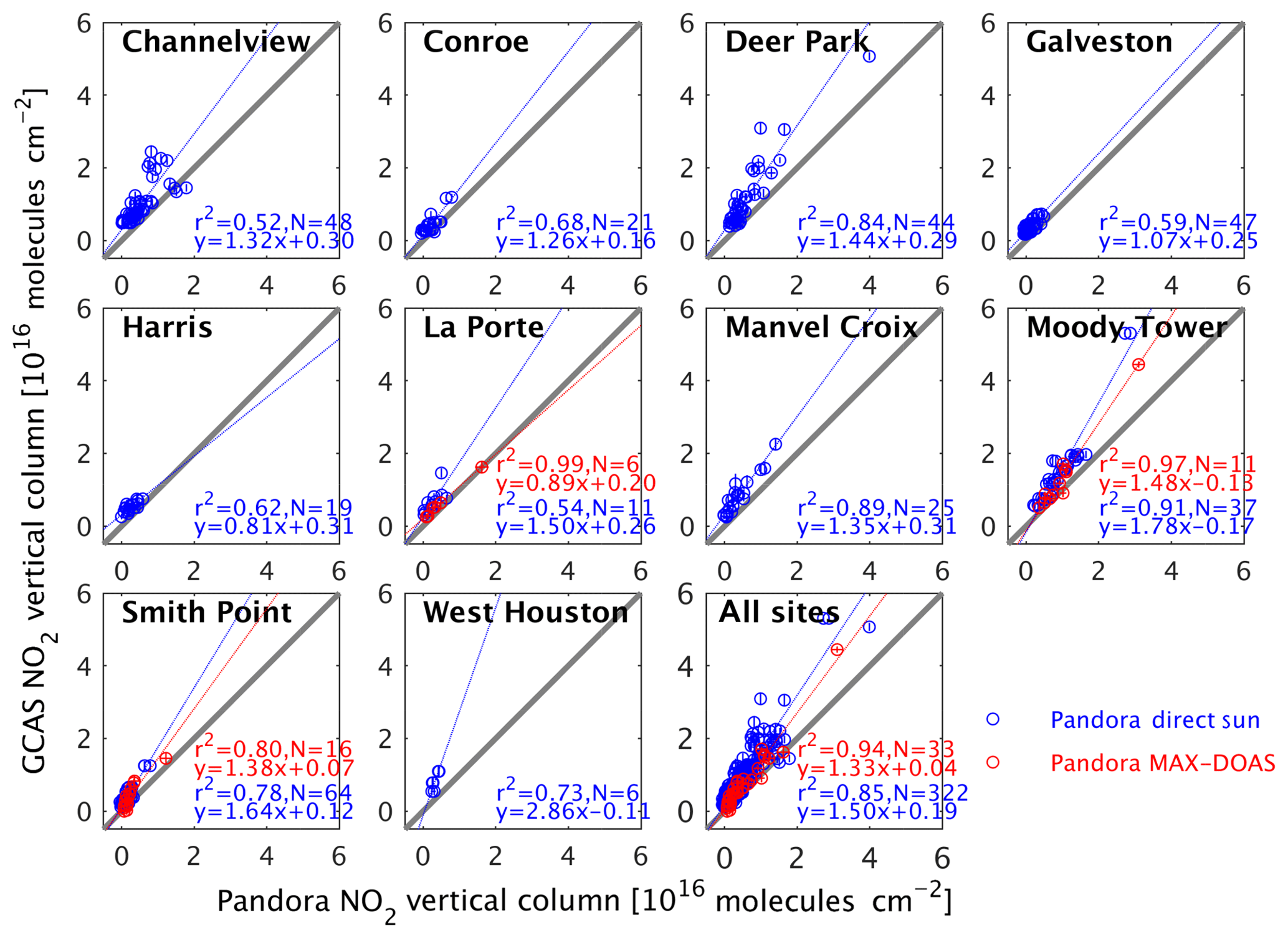
Figure 9Pandora NO₂ tropospheric columns from direct-sun and MAX-DOAS observations vs. GCAS NO₂ tropospheric columns by site for cloud-free observations over Houston during DISCOVER-AQ Texas 2013. The Pandora direct-sun columns are the total NO₂ columns measured by Pandora minus the colocated modeled stratospheric NO₂ columns used in the GCAS analysis. The solid line represents the 1 : 1 ratio. The dotted lines represent the reduced major axis linear regressions.

Download

Overall, GCAS tropospheric NO₂ is larger than Pandora (GCAS∕Pandora = 1.50 for DS and 1.33 for MAX-DOAS), although the spatial correlations are very good at r²=0.85 (DS) and r²=0.94 (MAX-DOAS). A background offset of $\sim 2 \times 10^{15}$ molecules cm⁻² is seen between GCAS and the Pandora DS measurements, similar to that seen in the P-3B comparisons. Again, this is most likely from uncertainties in the modeled stratospheric correction and reference spectrum correction, with a possible contribution from the Pandora reference as well. More surprisingly, GCAS NO₂ is 50 % (DS) and 33 % (MAX-DOAS) larger at high NO₂ values.

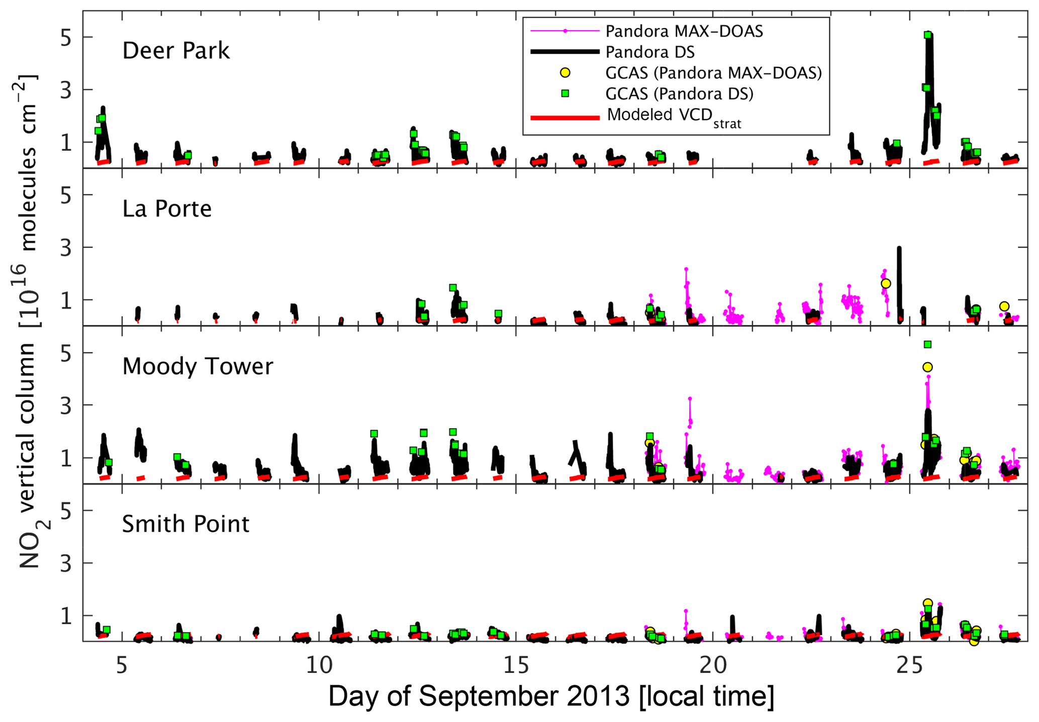
https://www.atmos-meas-tech.net/11/5941/2018/amt-11-5941-2018-f10

Figure 10Tropospheric NO₂ columns from Pandora direct-sun (DS) and MAX-DOAS observations as a function of time between 4 and 27 September at Deer Park, La Porte, Moody Tower and Smith Point sites, and GCAS coincidences with those observations, as well as stratospheric NO₂ from a model at Pandora DS measurements. Pandora DS tropospheric columns are derived by removing the modeled stratosphere from the retrieved Pandora total columns.

Download

6.3 AMF from P-3B profiles

In order to assess the dependence of the GCAS observations on the profile uncertainty, we also apply the P-3B profiles in place of model profiles in the GCAS AMF calculations and compare the new GCAS columns with the P-3B and Pandora columns. When the spiral profiles are applied to the GCAS observations within their vicinity, the use of the observed profiles lowers the overall slope of GCAS tropospheric NO₂ columns by 4 % (P-3B) and 2 % (Pandora) and the CH₂O columns by 2 % (P-3B) as compared with coincident observations. The NO₂ correlations with the P-3B and Pandora remain the same, but the correlation increases to r²=0.62 for P-3B CH₂O. Individual coincident observations can change by as much as −50 % to +35 % for NO₂ (mean change of $+ 1 \pm 10$ %) and −15 % to +25 % for CH₂O (mean change of $+ 3 \pm 8$ %). The largest mean changes for a single day occur at the Deer Park site in the Pandora comparisons, where the GCAS NO₂ column on 25 September is reduced by 15 % on average.

6.4 Discussion of coincident measurement comparisons

Overall, the GCAS observations correlate well spatially and temporally with the P-3B and Pandora observations. The GCAS observations also show agreement in magnitude with the P-3B-inferred NO₂ and CH₂O columns well within the measurement uncertainties. The GCAS NO₂ observations are significantly higher than those of the Pandora direct-sun instruments by 50 %. They are also higher than the Pandora MAX-DOAS by 33 %, although there are fewer coincidences with the MAX-DOAS observations, and there is good agreement at the La Porte site.

Differences between GCAS and the P-3B primarily result from errors in the GCAS AMF (surface reflectance, aerosols and profile shape); the inability of the P-3B to capture profiles of near-surface gases below 300 m near the Channelview, Manvel Croix and Moody Tower sites; and spatial variability and P-3B sampling. Much of the variability observed in individual spirals in the NO₂ column comparison in Fig. 7 is due to the large radius of the P-3B spiral, which can mean the P-3B sometimes flies in and out of NO₂ plumes, as seen in Fig. 5.

The differences between GCAS and Pandora NO₂ are much larger. GCAS NO₂ columns could be influenced by several uncertainties that can result in cumulative biases in the AMF calculation (again, primarily from errors in surface reflectance, aerosols and profile shape). Different factors likely dominate the uncertainties at different sites; some sites are located at locations with very inhomogeneous surface reflectance (Smith Point and Moody Tower), and some at locations with large uncertainties in profile shape. The slope is also dominated by the larger polluted measurements on 25 September, which was a day with complicated meteorology, a morning boundary layer of ∼200 m (according to HSRL data) and uncertain emissions (Souri et al., 2018).

Souri et al. (2018) also found a large difference between GCAS and Pandora observations during the Texas campaign. By using a Bayesian inversion to constrain the MODIS BRDF, they reduced the overestimation of GCAS relative to Pandora by 23 % through a 0.023 increase in surface albedo, broadly consistent with studies that have found a low bias in MODIS surface reflectance (Salomon et al., 2006; Y. Wang et al., 2010) at short wavelengths. The exclusion of aerosols in our AMF calculation may cause the AMF to be underestimated (and therefore the vertical column to be overestimated) in some cases, particularly where scattering aerosols are in the lowest part of the boundary layer (see discussion in Sect. 4.5.2). We find that the GCAS vertical columns at Pandora coincidences are reduced on average by 10 % when the air mass factor is calculated using the nearest HSRL aerosol optical thickness profiles below the aircraft for scattering aerosols. In the previous section, we saw there is likely a small +2 % bias in the GCAS column from the use of CMAQ-modeled NO₂ profile shapes in measurements coincident with Pandora. Therefore, while profile shape may contribute to large errors on individual observations, it is unlikely to produce a large bias in the GCAS observations overall.

Differences in the GCAS and Pandora slant column retrievals themselves may also play a role, including the wavelength fitting region and atmospheric temperature assumptions. Previous comparisons of Pandora DS total column NO₂ observations with other ground-based observations have shown good agreement (Herman et al., 2009; S. Wang et al., 2010). In contrast, Knepp et al. (2017) compared a year of Pandora zenith sky stratospheric NO₂ slant columns with those from a zenith-looking UV–Vis spectrometer (DOAS M07) from the Network for the Detection of Atmospheric Composition Change (NDACC) using different retrieval settings and found Pandora underestimated the NDACC instrument by 7 %–40 %. The Pandora slant column product used in our study was produced assuming a fixed effective temperature of 264 K, which could result in a low bias in the retrieved Pandora slant column of 10 % (Spinei et al., 2014).

Despite the sources of uncertainty on the GCAS columns, it should be noted that a large reduction in the GCAS vertical columns from the use of different AMF inputs resulting in better agreement with the Pandora columns would mean a significant underestimation by GCAS of both the NO₂ and CH₂O P-3B columns. Recent comparisons of Pandora DS NO₂ columns and NO₂ inferred from the P-3B P-CL instrument for the four DISCOVER-AQ campaigns (Maryland, California, Texas and Colorado) show the P-3B agrees well with Pandora DS measurements for all campaigns except Texas, where Pandora NO₂ is significantly underestimated (Sungyeon Choi, personal communication). Previous airborne comparisons with the GeoTASO instrument during DISCOVER-AQ Texas on four relatively unpolluted or cloudy days (13, 14, 18, 24 September) also suggested airborne NO₂ larger than Pandora (Nowlan et al., 2016).

7 Conclusions

We have presented trace gas retrievals of NO₂ and CH₂O from the GCAS instrument during the DISCOVER-AQ Texas 2013 campaign. In these retrievals, we first use a spectral fit to derive slant column densities from nadir spectra, in combination with reference spectra measured over a clean area. We then convert those slant columns to vertical columns using tropospheric trace gas profiles from the CMAQ model and surface reflectance from the MODIS BRDF product. At a spatial resolution of 250 m × 500 m, the NO₂ product has a mean precision of 1×10¹⁵ molecules cm⁻², and the CH₂O product has a mean precision of 1.9×10¹⁶ molecules cm⁻². In order to meet TEMPO precision requirements, and to detect enhanced CH₂O during the DISCOVER-AQ Texas campaign, we recommend CH₂O be spatially averaged to 1 km². Uncertainties in NO₂ polluted observations are dominated by air mass factor uncertainties, which result primarily from uncertainties in surface reflectance, aerosol loading and trace gas profile shape. These air mass factor uncertainties also play a role in individual CH₂O uncertainties but can be similar in magnitude to uncertainties from spectral fitting noise.

Comparisons between GCAS and P-3B and Pandora observations show GCAS data are very well correlated with these coincident measurements, but in some cases they show differences in magnitude. GCAS columns agree well with those inferred from P-3B in situ profiles for both NO₂ (r²=0.89; GCAS∕P-3B slope = 0.90 and intercept $= 1.6 \times 10^{15}$ molecules cm⁻²) and CH₂O (r²=0.54; GCAS∕P-3B slope=1.08 and intercept $= - 5 \times 10^{14}$ molecules cm⁻²). The use of P-3B profiles instead of modeled profile shapes results in a mean difference of 2 %–4 % in GCAS columns in comparisons with coincident observations. GCAS is higher than Pandora MAX-DOAS tropospheric NO₂ columns but shows excellent spatial agreement (r²=0.94; GCAS∕Pandora slope = 1.33 and intercept $= 4 \times 10^{14}$ molecules cm⁻²); these differences in magnitude, however, remain within the bounds of GCAS systematic error estimates in the AMF. The largest discrepancies in magnitude are seen between GCAS and Pandora direct-sun observations, although spatial correlations are very good (r²=0.85; GCAS∕Pandora slope = 1.50 and intercept $= 1.9 \times 10^{15}$ molecules cm⁻²). As both Pandora and GCAS are key instruments in planned TEMPO validation activities, there is clearly a need to resolve these differences in magnitude to ensure reliable validation studies. Further opportunities for comparisons over different geographic areas and pollution regimes exist in other campaigns.

Since DISCOVER-AQ Texas in 2013, the airborne GCAS and GeoTASO instruments have been deployed in the DISCOVER-AQ Colorado field campaign (2014), KORUS-AQ field campaign (2016), GOES-R validation campaign (2017), Lake Michigan Ozone Study (2017) and Long Island Sound Tropospheric Ozone Study (2018). These data are currently under study and offer further opportunities to examine the effects of surface characterization, profile shape, aerosols, viewing geometries and trace gas heterogeneity on ground, airborne and satellite remotely sensed trace gas columns.

Data availability

The GCAS and P-3B NO₂ and C₂HO data and Pandora direct-sun NO₂ columns are publicly available from the DISCOVER-AQ data archive at http://www-air.larc.nasa.gov/missions/discover-aq/discover-aq.html (last access: 23 October 2018) (Nowlan et al., 2017). The archived GCAS data also include coincident model profiles for each observation.

Author contributions

CRN performed the slant column retrievals, air mass factor calculations and instrument comparisons, and wrote the manuscript. CRN, XL and KC initiated and designed the research. SJJ and MGK collected and calibrated the GCAS spectra. HAK assisted in the analysis of spectra and slant column retrievals. GGA provided the radiative transfer model and guided interpretations. MBFC, CPL and KEP provided the CMAQ model simulations. AF, DR, JW, PW and AJW collected and provided the P-3B in situ aircraft data. JRH and ES provided the Pandora data. LMJ provided in situ data for correcting Pandora observations at Moody Tower. All authors contributed to interpretations and edited the manuscript.

Competing interests

The authors declare that they have no conflict of interest.

Acknowledgements

This study was supported under NASA grants NNX14AR69G and NNX17AE09G. MODIS MCD43GF V005 data were provided by the MODIS remote-sensing group at the University of Massachusetts Boston. We thank Amir Souri for helpful discussions.

Edited by: Michel Van Roozendael
Reviewed by: two anonymous referees

References

Aliwell, S. R., Van Roozendael, M., Johnston, P. V., Richter, A., Wagner, T., Arlander, D. W., Burrows, J. P., Fish, D. J., Jones, R. L., Tørnkvist, K. K., Lambert, J.-C., Pfeilsticker, K., and Pundt, I.: Analysis for BrO in zenith-sky spectra: An intercomparison exercise for analysis improvement, J. Geophys. Res.-Atmos., 107, 4199, https://doi.org/10.1029/2001JD000329, 2002. a

Baidar, S., Oetjen, H., Coburn, S., Dix, B., Ortega, I., Sinreich, R., and Volkamer, R.: The CU Airborne MAX-DOAS instrument: vertical profiling of aerosol extinction and trace gases, Atmos. Meas. Tech., 6, 719–739, https://doi.org/10.5194/amt-6-719-2013, 2013. a

Barkley, M. P., Palmer, P. I., Kuhn, U., Kesselmeier, J., Chance, K., Kurosu, T. P., Martin, R. V., Helmig, D., and Guenther, A.: Net ecosystem fluxes of isoprene over tropical South America inferred from Global Ozone Monitoring Experiment (GOME) observations of HCHO columns, J. Geophys. Res.-Atmos., 113, D20304, https://doi.org/10.1029/2008JD009863, 2008. a

Beirle, S., Lampel, J., Lerot, C., Sihler, H., and Wagner, T.: Parameterizing the instrumental spectral response function and its changes by a super-Gaussian and its derivatives, Atmos. Meas. Tech., 10, 581–598, https://doi.org/10.5194/amt-10-581-2017, 2017. a

Boersma, K. F., Eskes, H. J., and Brinksma, E. J.: Error analysis for tropospheric NO₂ retrieval from space, J. Geophys. Res.-Atmos., 109, D04311, https://doi.org/10.1029/2003JD003962, 2004. a, b, c

Boersma, K. F., Jacob, D. J., Eskes, H. J., Pinder, R. W., Wang, J., and van der A, R. J.: Intercomparison of SCIAMACHY and OMI tropospheric NO₂ columns: Observing the diurnal evolution of chemistry and emissions from space, J. Geophys. Res.-Atmos., 113, D16S26, https://doi.org/10.1029/2007JD008816, 2008. a

Bourassa, A. E., McLinden, C. A., Sioris, C. E., Brohede, S., Bathgate, A. F., Llewellyn, E. J., and Degenstein, D. A.: Fast NO₂ retrievals from Odin-OSIRIS limb scatter measurements, Atmos. Meas. Tech., 4, 965–972, https://doi.org/10.5194/amt-4-965-2011, 2011. a

Brion, J., Chakir, A., Daumont, D., Malicet, J., and Parisse, C.: High-resolution laboratory absorption cross section of O₃. Temperature effect, Chem. Phys. Lett., 213, 610–612, 1993. a, b, c

Broccardo, S., Heue, K.-P., Walter, D., Meyer, C., Kokhanovsky, A., van der A, R., Piketh, S., Langerman, K., and Platt, U.: Intra-pixel variability in satellite tropospheric NO₂ column densities derived from simultaneous space-borne and airborne observations over the South African Highveld, Atmos. Meas. Tech., 11, 2797–2819, https://doi.org/10.5194/amt-11-2797-2018, 2018. a

Bucsela, E. J., Krotkov, N. A., Celarier, E. A., Lamsal, L. N., Swartz, W. H., Bhartia, P. K., Boersma, K. F., Veefkind, J. P., Gleason, J. F., and Pickering, K. E.: A new stratospheric and tropospheric NO₂ retrieval algorithm for nadir-viewing satellite instruments: applications to OMI, Atmos. Meas. Tech., 6, 2607–2626, https://doi.org/10.5194/amt-6-2607-2013, 2013. a

Byun, D. and Schere, K. L.: Review of the governing equations, computational algorithms, and other components of the Models-3 Community Multiscale Air Quality (CMAQ) modeling system, Appl. Mech. Rev., 59, 51–77, https://doi.org/10.1115/1.2128636, 2006. a

Cai, Z., Liu, Y., Liu, X., Chance, K., Nowlan, C. R., Lang, R., Munro, R., and Suleiman, R.: Characterization and correction of Global Ozone Monitoring Experiment 2 ultraviolet measurements and application to ozone profile retrievals, J. Geophys. Res.-Atmos., 117, D07305, https://doi.org/10.1029/2011JD017096, 2012. a, b

Chan Miller, C., Gonzalez Abad, G., Wang, H., Liu, X., Kurosu, T., Jacob, D. J., and Chance, K.: Glyoxal retrieval from the Ozone Monitoring Instrument, Atmos. Meas. Tech., 7, 3891–3907, https://doi.org/10.5194/amt-7-3891-2014, 2014. a

Chance, K.: Analysis of BrO measurements from the Global Ozone Monitoring Experiment, Geophys. Res. Lett., 25, 3335–3338, https://doi.org/10.1029/98GL52359, 1998. a

Chance, K. and Kurucz, R. L.: An improved high-resolution solar reference spectrum for Earth's atmosphere measurements in the ultraviolet, visible, and near infrared, J. Quant. Spectrosc. Ra., 111, 1289–1295, https://doi.org/10.1016/j.jqsrt.2010.01.036, 2010. a

Chance, K. and Orphal, J.: Revised ultraviolet absorption cross sections of H₂CO for the HITRAN database, J. Quant. Spectrosc. Ra., 112, 1509–1510, https://doi.org/10.1016/j.jqsrt.2011.02.002, 2011. a, b

Chance, K., Palmer, P. I., Spurr, R. J., Martin, R. V., Kurosu, T. P., and Jacob, D. J.: Satellite observations of formaldehyde over North America from GOME, Geophys. Res. Lett., 27, 3461–3464, 2000. a, b

Chance, K., Kurosu, T. P., and Sioris, C. E.: Undersampling correction for array detector-based satellite spectrometers, Appl. Optics, 44, 1296–1304, https://doi.org/10.1364/AO.44.001296, 2005. a, b, c

Chance, K., Liu, X., Suleiman, R. M., Flittner, D. E., Al-Saadi, J., and Janz, S. J.: Tropospheric emissions: monitoring of pollution (TEMPO), Proc. SPIE, 8866, 88660D, https://doi.org/10.1117/12.2024479, 2013. a

Chance, K. V. and Spurr, R. J. D.: Ring effect studies: Rayleigh scattering, including molecular parameters for rotational Raman scattering, and the Fraunhofer spectrum, Appl. Optics, 36, 5224–5230, 1997. a, b, c

Chimot, J., Vlemmix, T., Veefkind, J. P., de Haan, J. F., and Levelt, P. F.: Impact of aerosols on the OMI tropospheric NO₂ retrievals over industrialized regions: how accurate is the aerosol correction of cloud-free scenes via a simple cloud model?, Atmos. Meas. Tech., 9, 359–382, https://doi.org/10.5194/amt-9-359-2016, 2016. a

Crawford, J., Pierce, G., Long, R., Szykman, J., Leitch, J., Nowlan, C., Herman, J., Weinheimer, A., and Al-Saadi, J.: Multi-perspective observations of NO₂ over the Denver area during DISCOVER-AQ: Insights for future monitoring, EM Magazine, 66, 25–29, 2016. a

De Smedt, I., Müller, J.-F., Stavrakou, T., van der A, R., Eskes, H., and Van Roozendael, M.: Twelve years of global observations of formaldehyde in the troposphere using GOME and SCIAMACHY sensors, Atmos. Chem. Phys., 8, 4947–4963, https://doi.org/10.5194/acp-8-4947-2008, 2008. a

De Smedt, I., Van Roozendael, M., Stavrakou, T., Müller, J.-F., Lerot, C., Theys, N., Valks, P., Hao, N., and van der A, R.: Improved retrieval of global tropospheric formaldehyde columns from GOME-2/MetOp-A addressing noise reduction and instrumental degradation issues, Atmos. Meas. Tech., 5, 2933–2949, https://doi.org/10.5194/amt-5-2933-2012, 2012. a

Fishman, J., Iraci, L. T., Al-Saadi, J., Chance, K., Chavez, F., Chin, M., Coble, P., Davis, C., DiGiacomo, P. M., Edwards, D., Eldering, A., Goes, J., Herman, J., Hu, C., Jacob, D. J., Jordan, C., Kawa, S. R., Key, R., Liu, X., Lohrenz, S., Mannino, A., Natraj, V., Neil, D., Neu, J., Newchurch, M., Pickering, K., Salisbury, J., Sosik, H., Subramaniam, A., Tzortziou, M., Wang, J., and Wang, M.: The United States' next generation of atmospheric composition and coastal ecosystem measurements: NASA's Geostationary Coastal and Air Pollution Events (GEO-CAPE) Mission, B. Am. Meteorol. Soc., 93, 1547–1566, https://doi.org/10.1175/bams-d-11-00201.1, 2012. a

Flynn, L., Long, C., Wu, X., Evans, R., Beck, C. T., Petropavlovskikh, I., McConville, G., Yu, W., Zhang, Z., Niu, J., Beach, E., Hao, Y., Pan, C., Sen, B., Novicki, M., Zhou, S., and Seftor, C.: Performance of the Ozone Mapping and Profiler Suite (OMPS) products, J. Geophys. Res.-Atmos., 119, 6181–6195, https://doi.org/10.1002/2013JD020467, 2014. a

Fowler, D., Coyle, M., Skiba, U., Sutton, M. A., Cape, J. N., Reis, S., Sheppard, L. J., Jenkins, A., Grizzetti, B., Galloway, J. N., Vitousek, P., Leach, A., Bouwman, A. F., Butterbach-Bahl, K., Dentener, F., Stevenson, D., Amann, M., and Voss, M.: The global nitrogen cycle in the twenty-first century, Philos. T. Roy. Soc. B, 368, 20130164, https://doi.org/10.1098/rstb.2013.0164, 2013. a

Fried, A., Olson, J. R., Walega, J. G., Crawford, J. H., Chen, G., Weibring, P., Richter, D., Roller, C., Tittel, F., Porter, M., Fuelberg, H., Halland, J., Bertram, T. H., Cohen, R. C., Pickering, K., Heikes, B. G., Snow, J. A., Shen, H., O'Sullivan, D. W., Brune, W. H., Ren, X., Blake, D. R., Blake, N., Sachse, G., Diskin, G. S., Podolske, J., Vay, S. A., Shetter, R. E., Hall, S. R., Anderson, B. E., Thornhill, L., Clarke, A. D., McNaughton, C. S., Singh, H. B., Avery, M. A., Huey, G., Kim, S., and Millet, D. B.: Role of convection in redistributing formaldehyde to the upper troposphere over North America and the North Atlantic during the summer 2004 INTEX campaign, J. Geophys. Res.-Atmos., 113, D107306, https://doi.org/10.1029/2007JD009760, 2008. a

Fried, A., Cantrell, C., Olson, J., Crawford, J. H., Weibring, P., Walega, J., Richter, D., Junkermann, W., Volkamer, R., Sinreich, R., Heikes, B. G., O'Sullivan, D., Blake, D. R., Blake, N., Meinardi, S., Apel, E., Weinheimer, A., Knapp, D., Perring, A., Cohen, R. C., Fuelberg, H., Shetter, R. E., Hall, S. R., Ullmann, K., Brune, W. H., Mao, J., Ren, X., Huey, L. G., Singh, H. B., Hair, J. W., Riemer, D., Diskin, G., and Sachse, G.: Detailed comparisons of airborne formaldehyde measurements with box models during the 2006 INTEX-B and MILAGRO campaigns: potential evidence for significant impacts of unmeasured and multi-generation volatile organic carbon compounds, Atmos. Chem. Phys., 11, 11867–11894, https://doi.org/10.5194/acp-11-11867-2011, 2011. a

Fried, A., Barth, M., Bela, M., Weibring, P., Richter, D., Walega, J., Li, Y., Pickering, K., Apel, E., Hornbrook, R., Hills, A., Riemer, D. D., Blake, N., Blake, D., Schroeder, J. R., Luo, Z. J., Crawford, J. H., Olson, J., Rutledge, S., Betten, D., Biggerstaff, M. I., Diskin, G., Sachse, G., Campos, T., Flocke, F., Weinheimer, A., Cantrell, C., Pollack, I., Peischl, J., Froyd, K., Wisthaler, A., Mikoviny, T., and Woods, S.: Convective transport of formaldehyde to the upper troposphere and lower stratosphere and associated scavenging in thunderstorms over the central United States during the 2012 DC3 study, J. Geophys. Res.-Atmos., 121, 7430–7460, https://doi.org/10.1002/2015JD024477, 2016a. a

Fried, A., Loughner, C. P., and Pickering, K.: Analysis of Airborne Formaldehyde Data Over Houston Texas Acquired During the 2013 DISCOVER-AQ and SEAC⁴RS Campaigns, final Report to Texas AQRP, Project 14-002, available at: http://aqrp.ceer.utexas.edu/projectinfoFY14_15/14-002/14-002 Final Report.pdf (last access: 23 October 2018), 2016b. a, b, c, d, e, f

Fried, A., Walega, J., Weibring, P., Richter, D., Nowlan, C., Liu, X., Janz, S., Kowalewski, M., Chance, K., Abad, G. G., Wisthaler, A., Mikoviny, T., Diskin, G., Al-Saadi, J., Crawford, J., and Loughner, C.: Derived formaldehyde vertical columns during the DISCOVER-AQ campaigns and detailed comparisons of in-situ measurements onboard the NASA WP3 aircraft with remote column measurements from GCAS and OMI instruments, in preparation, 2018. a

González Abad, G., Liu, X., Chance, K., Wang, H., Kurosu, T. P., and Suleiman, R.: Updated Smithsonian Astrophysical Observatory Ozone Monitoring Instrument (SAO OMI) formaldehyde retrieval, Atmos. Meas. Tech., 8, 19–32, https://doi.org/10.5194/amt-8-19-2015, 2015. a, b

González Abad, G., Vasilkov, A., Seftor, C., Liu, X., and Chance, K.: Smithsonian Astrophysical Observatory Ozone Mapping and Profiler Suite (SAO OMPS) formaldehyde retrieval, Atmos. Meas. Tech., 9, 2797–2812, https://doi.org/10.5194/amt-9-2797-2016, 2016. a, b

Hair, J. W., Hostetler, C. A., Cook, A. L., Harper, D. B., Ferrare, R. A., Mack, T. L., Welch, W., Izquierdo, L. R., and Hovis, F. E.: Airborne High Spectral Resolution Lidar for profiling aerosol optical properties, Appl. Optics, 47, 6734–6752, https://doi.org/10.1364/AO.47.006734, 2008. a

Herman, J., Cede, A., Spinei, E., Mount, G., Tzortziou, M., and Abuhassan, N.: NO₂ column amounts from ground-based Pandora and MFDOAS spectrometers using the direct-sun DOAS technique: Intercomparisons and application to OMI validation, J. Geophys. Res.-Atmos., 114, D13307, https://doi.org/10.1029/2009JD011848, 2009. a, b, c, d

Heue, K.-P., Wagner, T., Broccardo, S. P., Walter, D., Piketh, S. J., Ross, K. E., Beirle, S., and Platt, U.: Direct observation of two dimensional trace gas distributions with an airborne Imaging DOAS instrument, Atmos. Chem. Phys., 8, 6707–6717, https://doi.org/10.5194/acp-8-6707-2008, 2008. a

Hoek, G., Krishnan, R. M., Beelen, R., Peters, A., Ostro, B., Brunekreef, B., and Kaufman, J. D.: Long-term air pollution exposure and cardio-respiratory mortality: a review, Environ. Health, 12, 43, https://doi.org/10.1186/1476-069X-12-43, 2013. a

Kleipool, Q. L., Dobber, M. R., de Haan, J. F., and Levelt, P. F.: Earth surface reflectance climatology from 3 years of OMI data, J. Geophys. Res.-Atmos., 113, D18308, https://doi.org/10.1029/2008JD010290, 2008. a

Knepp, T. N., Querel, R., Johnston, P., Thomason, L., Flittner, D., and Zawodny, J. M.: Intercomparison of Pandora stratospheric NO₂ slant column product with the NDACC-certified M07 spectrometer in Lauder, New Zealand, Atmos. Meas. Tech., 10, 4363–4372, https://doi.org/10.5194/amt-10-4363-2017, 2017. a

Kowalewski, M. G. and Janz, S. J.: Remote sensing capabilities of the GEO-CAPE airborne simulator, Proc. SPIE, 9218, 92181I, https://doi.org/10.1117/12.2062058, 2014. a, b, c, d, e

Kuhlmann, G., Hueni, A., Damm, A., and Brunner, D.: An algorithm for in-flight spectral calibration of imaging spectrometers, Remote Sens., 8, https://doi.org/10.3390/rs8121017, 2016. a

Kwon, H.-A., Park, R. J., Jeong, J. I., Lee, S., González Abad, G., Kurosu, T. P., Palmer, P. I., and Chance, K.: Sensitivity of formaldehyde (HCHO) column measurements from a geostationary satellite to temporal variation of the air mass factor in East Asia, Atmos. Chem. Phys., 17, 4673–4686, https://doi.org/10.5194/acp-17-4673-2017, 2017. a

Lamsal, L. N., Krotkov, N. A., Celarier, E. A., Swartz, W. H., Pickering, K. E., Bucsela, E. J., Gleason, J. F., Martin, R. V., Philip, S., Irie, H., Cede, A., Herman, J., Weinheimer, A., Szykman, J. J., and Knepp, T. N.: Evaluation of OMI operational standard NO₂ column retrievals using in situ and surface-based NO₂ observations, Atmos. Chem. Phys., 14, 11587–11609, https://doi.org/10.5194/acp-14-11587-2014, 2014. a, b

Lamsal, L. N., Janz, S. J., Krotkov, N. A., Pickering, K. E., Spurr, R. J. D., Kowalewski, M. G., Loughner, C. P., Crawford, J. H., Swartz, W. H., and Herman, J. R.: High-resolution NO₂ observations from the Airborne Compact Atmospheric Mapper: Retrieval and validation, J. Geophys. Res.-Atmos., 122, 1953–1970, https://doi.org/10.1002/2016JD025483, 2017. a, b

Lawrence, J. P., Anand, J. S., Vande Hey, J. D., White, J., Leigh, R. R., Monks, P. S., and Leigh, R. J.: High-resolution measurements from the airborne Atmospheric Nitrogen Dioxide Imager (ANDI), Atmos. Meas. Tech., 8, 4735–4754, https://doi.org/10.5194/amt-8-4735-2015, 2015. a

Leitão, J., Richter, A., Vrekoussis, M., Kokhanovsky, A., Zhang, Q. J., Beekmann, M., and Burrows, J. P.: On the improvement of NO₂ satellite retrievals – aerosol impact on the airmass factors, Atmos. Meas. Tech., 3, 475–493, https://doi.org/10.5194/amt-3-475-2010, 2010. a

Levelt, P. F., van den Oord, G. H., Dobber, M. R., Malkki, A., Visser, H., de Vries, J., Stammes, P., Lundell, J. O., and Saari, H.: The ozone monitoring instrument, IEEE T. Geosci. Remote, 44, 1093–1101, 2006. a

Li, X., Choi, Y., Czader, B., Roy, A., Kim, H., Lefer, B., and Pan, S.: The impact of observation nudging on simulated meteorology and ozone concentrations during DISCOVER-AQ 2013 Texas campaign, Atmos. Chem. Phys., 16, 3127–3144, https://doi.org/10.5194/acp-16-3127-2016, 2016. a, b

Lin, J.-T., Martin, R. V., Boersma, K. F., Sneep, M., Stammes, P., Spurr, R., Wang, P., Van Roozendael, M., Clémer, K., and Irie, H.: Retrieving tropospheric nitrogen dioxide from the Ozone Monitoring Instrument: effects of aerosols, surface reflectance anisotropy, and vertical profile of nitrogen dioxide, Atmos. Chem. Phys., 14, 1441–1461, https://doi.org/10.5194/acp-14-1441-2014, 2014. a, b

Liu, C., Liu, X., Kowalewski, M. G., Janz, S. J., González Abad, G., Pickering, K., Chance, K., and Lamsal, L. N.: Analysis of ACAM Data for Trace Gas Retrievals during the 2011 DISCOVER-AQ Campaign, J. Spectrosc., 2015, 827160, https://doi.org/10.1155/2015/827160, 2015a. a

Liu, C., Liu, X., Kowalewski, M. G., Janz, S. J., González Abad, G., Pickering, K. E., Chance, K., and Lamsal, L. N.: Characterization and verification of ACAM slit functions for trace-gas retrievals during the 2011 DISCOVER-AQ flight campaign, Atmos. Meas. Tech., 8, 751–759, https://doi.org/10.5194/amt-8-751-2015, 2015b. a, b, c, d, e, f

Liu, X., Chance, K., Sioris, C. E., Spurr, R. J. D., Kurosu, T. P., Martin, R. V., and Newchurch, M. J.: Ozone profile and tropospheric ozone retrievals from the Global Ozone Monitoring Experiment: Algorithm description and validation, J. Geophys. Res.-Atmos., 110, D20307, https://doi.org/10.1029/2005JD006240, 2005. a

Liu, X., Bhartia, P. K., Chance, K., Spurr, R. J. D., and Kurosu, T. P.: Ozone profile retrievals from the Ozone Monitoring Instrument, Atmos. Chem. Phys., 10, 2521–2537, https://doi.org/10.5194/acp-10-2521-2010, 2010. a

Lorente, A., Boersma, K. F., Yu, H., Dörner, S., Hilboll, A., Richter, A., Liu, M., Lamsal, L. N., Barkley, M., De Smedt, I., Van Roozendael, M., Wang, Y., Wagner, T., Beirle, S., Lin, J.-T., Krotkov, N., Stammes, P., Wang, P., Eskes, H. J., and Krol, M.: Structural uncertainty in air mass factor calculation for NO₂ and HCHO satellite retrievals, Atmos. Meas. Tech., 10, 759–782, https://doi.org/10.5194/amt-10-759-2017, 2017. a, b

Loughner, C. P. and Follette-Cook, M.: Emission source region contributions to a high surface ozone episode during DISCOVER-AQ, final Report to Texas AQRP, Project 14-004, available at: http://aqrp.ceer.utexas.edu/projectinfoFY14_15%5C14-004%5C14-004 Final Report.pdf (last access: 23 October 2018), 2015. a, b, c

Marais, E., Jacob, D., Wecht, K., Lerot, C., Zhang, L., Yu, K., Kurosu, T., Chance, K., and Sauvage, B.: Anthropogenic emissions in Nigeria and implications for atmospheric ozone pollution: A view from space, Atmos. Environ., 99, 32–40, https://doi.org/10.1016/j.atmosenv.2014.09.055, 2014. a

Martin, R. V., Chance, K., Jacob, D. J., Kurosu, T. P., Spurr, R. J. D., Bucsela, E., Gleason, J. F., Palmer, P. I., Bey, I., Fiore, A. M., Li, Q., Yantosca, R. M., and Koelemeijer, R. B. A.: An improved retrieval of tropospheric nitrogen dioxide from GOME, J. Geophys. Res.-Atmos., 107, 4437, https://doi.org/10.1029/2001JD001027, 2002. a, b

Mazzuca, G. M., Pickering, K. E., Clark, R. D., Loughner, C. P., Fried, A., Stein Zweers, D. C., Weinheimer, A. J., and Dickerson, R. R.: Use of tethersonde and aircraft profiles to study the impact of mesoscale and microscale meteorology on air quality, Atmos. Environ., 149, 55–69, https://doi.org/10.1016/J.ATMOSENV.2016.10.025, 2017. a

McLinden, C. A., Olsen, S. C., Hannegan, B., Wild, O., Prather, M. J., and Sundet, J.: Stratospheric ozone in 3-D models: A simple chemistry and the cross-tropopause flux, J. Geophys. Res.-Atmos., 105, 14653–14665, 2000. a

McLinden, C. A., Fioletov, V., Boersma, K. F., Kharol, S. K., Krotkov, N., Lamsal, L., Makar, P. A., Martin, R. V., Veefkind, J. P., and Yang, K.: Improved satellite retrievals of NO₂ and SO₂ over the Canadian oil sands and comparisons with surface measurements, Atmos. Chem. Phys., 14, 3637–3656, https://doi.org/10.5194/acp-14-3637-2014, 2014. a

Meier, A. C., Schönhardt, A., Bösch, T., Richter, A., Seyler, A., Ruhtz, T., Constantin, D.-E., Shaiganfar, R., Wagner, T., Merlaud, A., Van Roozendael, M., Belegante, L., Nicolae, D., Georgescu, L., and Burrows, J. P.: High-resolution airborne imaging DOAS measurements of NO₂ above Bucharest during AROMAT, Atmos. Meas. Tech., 10, 1831–1857, https://doi.org/10.5194/amt-10-1831-2017, 2017. a, b

Mills, I. C., Atkinson, R. W., Kang, S., Walton, H., and Anderson, H. R.: Quantitative systematic review of the associations between short-term exposure to nitrogen dioxide and mortality and hospital admissions, BMJ Open, 5, e006946, https://doi.org/10.1136/bmjopen-2014-006946, 2015. a

Nowlan, C. R., Liu, X., Weinheimer, A., Fried, A., and Herman, J.: DISCOVER-AQ Data (GCAS, P-3B in situ, Pandora direct sun), https://doi.org/10.5067/Aircraft/DISCOVER-AQ/Aerosol-TraceGas, 2017. a

Nowlan, C. R., Liu, X., Chance, K., Cai, Z., Kurosu, T. P., Lee, C., and Martin, R. V.: Retrievals of sulfur dioxide from the Global Ozone Monitoring Experiment 2 (GOME-2) using an optimal estimation approach: Algorithm and initial validation, J. Geophys. Res.-Atmos., 116, D18301, https://doi.org/10.1029/2011JD015808, 2011. a

Nowlan, C. R., Martin, R. V., Philip, S., Lamsal, L. N., Krotkov, N. A., Marais, E. A., Wang, S., and Zhang, Q.: Global dry deposition of nitrogen dioxide and sulfur dioxide inferred from space-based measurements, Global Biogeochem. Cy., 28, 1025–1043, https://doi.org/10.1002/2014GB004805, 2014. a

Nowlan, C. R., Liu, X., Leitch, J. W., Chance, K., González Abad, G., Liu, C., Zoogman, P., Cole, J., Delker, T., Good, W., Murcray, F., Ruppert, L., Soo, D., Follette-Cook, M. B., Janz, S. J., Kowalewski, M. G., Loughner, C. P., Pickering, K. E., Herman, J. R., Beaver, M. R., Long, R. W., Szykman, J. J., Judd, L. M., Kelley, P., Luke, W. T., Ren, X., and Al-Saadi, J. A.: Nitrogen dioxide observations from the Geostationary Trace gas and Aerosol Sensor Optimization (GeoTASO) airborne instrument: Retrieval algorithm and measurements during DISCOVER-AQ Texas 2013, Atmos. Meas. Tech., 9, 2647–2668, https://doi.org/10.5194/amt-9-2647-2016, 2016. a, b, c, d, e, f, g, h, i, j, k, l, m, n

Otte, T. L. and Pleim, J. E.: The Meteorology-Chemistry Interface Processor (MCIP) for the CMAQ modeling system: updates through MCIPv3.4.1, Geosci. Model Dev., 3, 243–256, https://doi.org/10.5194/gmd-3-243-2010, 2010. a

Palmer, P. I., Jacob, D. J., Chance, K., Martin, R. V., Spurr, R. J., Kurosu, T. P., Bey, I., Yantosca, R., Fiore, A., and Li, Q.: Air mass factor formulation for spectroscopic measurements from satellites: Application to formaldehyde retrievals from the Global Ozone Monitoring Experiment, J. Geophys. Res.-Atmos., 106, 14539–14550, https://doi.org/10.1029/2000JD900772, 2001. a

Pan, S., Choi, Y., Jeon, W., Roy, A., Westenbarger, D. A., and Kim, H. C.: Impact of high-resolution sea surface temperature, emission spikes and wind on simulated surface ozone in Houston, Texas during a high ozone episode, Atmos. Environ., 152, 362–376, https://doi.org/10.1016/j.atmosenv.2016.12.030, 2017. a

Popp, C., Brunner, D., Damm, A., Van Roozendael, M., Fayt, C., and Buchmann, B.: High-resolution NO₂ remote sensing from the Airborne Prism EXperiment (APEX) imaging spectrometer, Atmos. Meas. Tech., 5, 2211–2225, https://doi.org/10.5194/amt-5-2211-2012, 2012. a

Prather, M.: Catastrophic loss of stratospheric ozone in dense volcanic clouds, J. Geophys. Res.-Atmos., 97, 10187–10191, 1992. a

Richter, A., Begoin, M., Hilboll, A., and Burrows, J. P.: An improved NO₂ retrieval for the GOME-2 satellite instrument, Atmos. Meas. Tech., 4, 1147–1159, https://doi.org/10.5194/amt-4-1147-2011, 2011. a

Ridley, B. A. and Grahek, F. E.: A small, low flow, high sensitivity reaction vessel for NO chemiluminescence detectors, J. Atmos. Ocean. Tech., 7, 307–311, https://doi.org/10.1175/1520-0426(1990)007<0307:ASLFHS>2.0.CO;2, 1990. a

Rodgers, C.: Inverse methods for atmospheric sounding: theory and practice, World Scientific, River Edge, NJ, USA, 2000. a

Román, M. O., Gatebe, C. K., Schaaf, C. B., Poudyal, R., Wang, Z., and King, M. D.: Variability in surface BRDF at different spatial scales (30 m–500 m) over a mixed agricultural landscape as retrieved from airborne and satellite spectral measurements, Remote Sens. Environ., 115, 2184–2203, https://doi.org/10.1016/j.rse.2011.04.012, 2011. a

Rothman, L., Gordon, I., Babikov, Y., Barbe, A., Chris Benner, D., Bernath, P., Birk, M., Bizzocchi, L., Boudon, V., Brown, L., Campargue, A., Chance, K., Cohen, E. A., Coudert, L., Devi, V., Drouin, B. J., Fayt, A., Flaud, J.-M., Gamache, R., Harrison, J., Hartmann, J.-M., Hill, C., Hodges, J., Jacquemart, D., Jolly, A., Lamouroux, J., Le Roy, R., Li, G., Long, D., Lyulin, O., Mackie, C., Massie, S., Mikhailenko, S., Müller, H., Naumenko, O., Nikitin, A., Orphal, J., Perevalov, V., Perrin, A., Polovtseva, E., Richard, C., Smith, M., Starikova, E., Sung, K., Tashkun, S., Tennyson, J., Toon, G., Tyuterev, V., and Wagner, G.: The HITRAN 2012 molecular spectroscopic database, J. Quant. Spectrosc. Ra., 130, 4–50, https://doi.org/10.1016/j.jqsrt.2013.07.002, 2013. a

Salomon, J. G., Schaaf, C. B., Strahler, A. H., Gao, F., and Jin, Y.: Validation of the MODIS bidirectional reflectance distribution function and albedo retrievals using combined observations from the aqua and terra platforms, IEEE T. Geosci. Remote, 44, 1555–1565, https://doi.org/10.1109/TGRS.2006.871564, 2006. a

Sawamura, P., Moore, R. H., Burton, S. P., Chemyakin, E., Müller, D., Kolgotin, A., Ferrare, R. A., Hostetler, C. A., Ziemba, L. D., Beyersdorf, A. J., and Anderson, B. E.: HSRL-2 aerosol optical measurements and microphysical retrievals vs. airborne in situ measurements during DISCOVER-AQ 2013: an intercomparison study, Atmos. Chem. Phys., 17, 7229–7243, https://doi.org/10.5194/acp-17-7229-2017, 2017. a

Schaaf, C. B., Gao, F., Strahler, A. H., Lucht, W., Li, X., Tsang, T., Strugnell, N. C., Zhang, X., Jin, Y., Muller, J.-P., Lewis, P., Barnsley, M., Hobson, P., Disney, M., Roberts, G., Dunderdale, M., Doll, C., d'Entremont, R. P., Hu, B., Liang, S., Privette, J. L., and Roy, D.: First operational BRDF, albedo nadir reflectance products from MODIS, Remote Sens. Environ., 83, 135–148, https://doi.org/10.1016/S0034-4257(02)00091-3, 2002. a

Schönhardt, A., Altube, P., Gerilowski, K., Krautwurst, S., Hartmann, J., Meier, A. C., Richter, A., and Burrows, J. P.: A wide field-of-view imaging DOAS instrument for two-dimensional trace gas mapping from aircraft, Atmos. Meas. Tech., 8, 5113–5131, https://doi.org/10.5194/amt-8-5113-2015, 2015. a

Sioris, C., Kurosu, T., Martin, R., and Chance, K.: Stratospheric and tropospheric NO₂ observed by SCIAMACHY: first results, Adv. Space Res., 34, 780–785, https://doi.org/10.1016/j.asr.2003.08.066, 2004. a

Skamarock, W. C., Klemp, J. B., Dudhia, J., Gill, D. O., Barker, D. L., Duda, M. G., Huang, X.-Y., Wang, W., and Powers, J. G.: A description of the Advanced Research WRF version 3, Tech. Rep. NCAR/TN-475+STR, NCAR, Boulder, CO, USA, 2008. a

Souri, A. H., Choi, Y., Jeon, W., Li, X., Pan, S., Diao, L., and Westenbarger, D. A.: Constraining NO_x emissions using satellite NO₂ measurements during 2013 DISCOVER-AQ Texas campaign, Atmos. Environ., 131, 371–381, https://doi.org/10.1016/j.atmosenv.2016.02.020, 2016. a

Souri, A. H., Choi, Y., Pan, S., Curci, G., Nowlan, C. R., Janz, S. J., Kowalewski, M. G., Liu, J., Herman, J. R., Weinheimer, A. J., and Flynn, J. H.: First top-down estimates of anthropogenic NO₂ emissions using high-resolution airborne remote sensing observations, J. Geophys. Res.-Atmos., 123, 3269–3284, https://doi.org/10.1002/2017JD028009, 2018. a, b, c, d, e

Spinei, E., Cede, A., Swartz, W. H., Herman, J., and Mount, G. H.: The use of NO₂ absorption cross section temperature sensitivity to derive NO₂ profile temperature and stratospheric–tropospheric column partitioning from visible direct-sun DOAS measurements, Atmos. Meas. Tech., 7, 4299–4316, https://doi.org/10.5194/amt-7-4299-2014, 2014. a

Spurr, R.: LIDORT and VLIDORT: Linearized pseudo-spherical scalar and vector discrete ordinate radiative transfer models for use in remote sensing retrieval problems, in: Light Scattering Reviews 3: Light Scattering and Reflection, 229–275, Springer Berlin Heidelberg, Berlin, Heidelberg, Germany, https://doi.org/10.1007/978-3-540-48546-9_7, 2008. a, b

Spurr, R. J.: VLIDORT: A linearized pseudo-spherical vector discrete ordinate radiative transfer code for forward model and retrieval studies in multilayer multiple scattering media, J. Quant. Spectrosc. Ra., 102, 316–342, https://doi.org/10.1016/j.jqsrt.2006.05.005, 2006. a

Stavrakou, T., Müller, J.-F., Bauwens, M., De Smedt, I., Van Roozendael, M., De Mazière, M., Vigouroux, C., Hendrick, F., George, M., Clerbaux, C., Coheur, P.-F., and Guenther, A.: How consistent are top-down hydrocarbon emissions based on formaldehyde observations from GOME-2 and OMI?, Atmos. Chem. Phys., 15, 11861–11884, https://doi.org/10.5194/acp-15-11861-2015, 2015. a

Sun, K., Liu, X., Nowlan, C. R., Cai, Z., Chance, K., Frankenberg, C., Lee, R. A. M., Pollock, R., Rosenberg, R., and Crisp, D.: Characterization of the OCO-2 instrument line shape functions using on-orbit solar measurements, Atmos. Meas. Tech., 10, 939–953, https://doi.org/10.5194/amt-10-939-2017, 2017a. a

Sun, K., Liu, X., Huang, G., González Abad, G., Cai, Z., Chance, K., and Yang, K.: Deriving the slit functions from OMI solar observations and its implications for ozone-profile retrieval, Atmos. Meas. Tech., 10, 3677–3695, https://doi.org/10.5194/amt-10-3677-2017, 2017b. a

Sun, Q., Wang, Z., Li, Z., Erb, A., and Schaaf, C. B.: Evaluation of the global MODIS 30 arc-second spatially and temporally complete snow-free land surface albedo and reflectance anisotropy dataset, Int. J. Appl. Earth Obs., 58, 36–49, https://doi.org/10.1016/j.jag.2017.01.011, 2017. a

Tack, F., Merlaud, A., Iordache, M.-D., Danckaert, T., Yu, H., Fayt, C., Meuleman, K., Deutsch, F., Fierens, F., and Van Roozendael, M.: High-resolution mapping of the NO₂ spatial distribution over Belgian urban areas based on airborne APEX remote sensing, Atmos. Meas. Tech., 10, 1665–1688, https://doi.org/10.5194/amt-10-1665-2017, 2017. a

Tack, F., Merlaud, A., Meier, A. C., Vlemmix, T., Ruhtz, T., Iordache, M.-D., Ge, X., van der Wal, L., Schuettemeyer, D., Ardelean, M., Calcan, A., Schönhardt, A., Meuleman, K., Richter, A., and Van Roozendael, M.: Intercomparison of four airborne imaging DOAS systems for tropospheric NO₂ mapping – The AROMAPEX campaign, Atmos. Meas. Tech. Discuss., https://doi.org/10.5194/amt-2017-478, in review, 2018. a

Thalman, R. and Volkamer, R.: Temperature dependent absorption cross-sections of O₂−O₂ collision pairs between 340 and 630 nm and at atmospherically relevant pressure, Phys. Chem. Chem. Phys., 15, 15371–15381, https://doi.org/10.1039/c3cp50968k, 2013. a, b

Vandaele, A. C., Hermans, C., Simon, P. C., Carleer, M., Colin, R., Fally, S., Mérienne, M. F., Jenouvrier, A., and Coquart, B.: Measurements of the NO₂ absorption cross-section from 42 000 cm⁻¹ to 10 000 cm⁻¹ (238–1000 nm) at 220 K and 294 K, J. Quant. Spectrosc. Ra., 59, 171–184, 1998. a, b, c

Vlemmix, T., Ge, X., de Goeij, B. T. G., van der Wal, L. F., Otter, G. C. J., Stammes, P., Wang, P., Merlaud, A., Schüttemeyer, D., Meier, A. C., Veefkind, J. P., and Levelt, P. F.: Retrieval of tropospheric NO₂ columns over Berlin from high-resolution airborne observations with the spectrolite breadboard instrument, Atmos. Meas. Tech. Discuss., https://doi.org/10.5194/amt-2017-257, in review, 2017. a

Wagner, T., Apituley, A., Beirle, S., Dörner, S., Friess, U., Remmers, J., and Shaiganfar, R.: Cloud detection and classification based on MAX-DOAS observations, Atmos. Meas. Tech., 7, 1289–1320, https://doi.org/10.5194/amt-7-1289-2014, 2014. a

Wang, H., Liu, X., Chance, K., González Abad, G., and Chan Miller, C.: Water vapor retrieval from OMI visible spectra, Atmos. Meas. Tech., 7, 1901–1913, https://doi.org/10.5194/amt-7-1901-2014, 2014. a

Wang, S., Pongetti, T. J., Sander, S. P., Spinei, E., Mount, G. H., Cede, A., and Herman, J.: Direct Sun measurements of NO₂ column abundances from Table Mountain, California: Intercomparison of low- and high-resolution spectrometers, J. Geophys. Res.-Atmos., 115, D13305, https://doi.org/10.1029/2009JD013503, 2010. a

Wang, Y., Lyapustin, A. I., Privette, J. L., Cook, R. B., SanthanaVannan, S. K., Vermote, E. F., and Schaaf, C. L.: Assessment of biases in MODIS surface reflectance due to Lambertian approximation, Remote Sens. Environ., 114, 2791–2801, https://doi.org/10.1016/j.rse.2010.06.013, 2010. a, b

Weibring, P., Richter, D., Fried, A., Walega, J., and Dyroff, C.: Ultra-high-precision mid-IR spectrometer II: system description and spectroscopic performance, Appl. Phys. B, 85, 207–218, https://doi.org/10.1007/s00340-006-2300-4, 2006. a

Weibring, P., Richter, D., Walega, J. G., and Fried, A.: First demonstration of a high performance difference frequency spectrometer on airborne platforms, Opt. Express, 15, 13476–13495, https://doi.org/10.1364/OE.15.013476, 2007. a

Wilmouth, D. M., Hanisco, T. F., Donahue, N. M., and Anderson, J. G.: Fourier transform ultraviolet spectroscopy of the A²Π_3∕2 ← X²Π_3∕2 transition of BrO, J. Phys. Chem. A, 103, 8935–8945, https://doi.org/10.1021/jp991651o, 1999. a

Yang, K., Carn, S. A., Ge, C., Wang, J., and Dickerson, R. R.: Advancing measurements of tropospheric NO₂ from space: New algorithm and first global results from OMPS, Geophys. Res. Lett., 41, 4777–4786, https://doi.org/10.1002/2014GL060136, 2014. a

Zhu, L., Jacob, D. J., Mickley, L. J., Marais, E. A., Cohan, D. S., Yoshida, Y., Duncan, B. N., González Abad, G., and Chance, K. V.: Anthropogenic emissions of highly reactive volatile organic compounds in eastern Texas inferred from oversampling of satellite (OMI) measurements of HCHO columns, Environ. Res. Lett., 9, 114004, https://doi.org/10.1088/1748-9326/9/11/114004, 2014. a, b

Zoogman, P., Liu, X., Suleiman, R., Pennington, W., Flittner, D., Al-Saadi, J., Hilton, B., Nicks, D., Newchurch, M., Carr, J., Janz, S., Andraschko, M., Arola, A., Baker, B., Canova, B., Chan Miller, C., Cohen, R. C., Davis, J., Dussault, M., Edwards, D., Fishman, J., Ghulam, A., González Abad, G., Grutter, M., Herman, J., Houck, J., Jacob, D., Joiner, J., Kerridge, B., Kim, J., Krotkov, N., Lamsal, L., Li, C., Lindfors, A., Martin, R., McElroy, C., McLinden, C., Natraj, V., Neil, D., Nowlan, C., O'Sullivan, E., Palmer, P., Pierce, R., Pippin, M., Saiz-Lopez, A., Spurr, R., Szykman, J., Torres, O., Veefkind, J., Veihelmann, B., Wang, H., Wang, J., and Chance, K.: Tropospheric emissions: Monitoring of pollution (TEMPO), J. Quant. Spectrosc. Ra., 186, 17–39, https://doi.org/10.1016/j.jqsrt.2016.05.008, 2017. a, b

Articles

Short summary

The GEO-CAPE Airborne Simulator (GCAS) was developed in support of future air quality and ocean color geostationary satellite missions. GCAS flew in its first field campaign on NASA's King Air B-200 aircraft during DISCOVER-AQ Texas in 2013. In this paper, we determine nitrogen dioxide and formaldehyde columns over Houston from the GCAS air quality sensor and compare those results with measurements made from ground-based Pandora spectrometers and in situ airborne instruments.

Nitrogen dioxide and formaldehyde measurements from the GEOstationary Coastal and Air Pollution Events (GEO-CAPE) Airborne Simulator over Houston, Texas

3.1 GCAS observations

3.2 Pandora observations

3.3 P-3B aircraft observations

3.4 Model simulations

4.1 Spectral calibration

4.2 Slant column retrieval

4.2.1 Spectral fitting

4.2.2 Reference spectrum

4.2.3 NO2 and CH2O fitting

4.3 Conversion to vertical column

4.3.1 Air mass factor calculation

4.3.2 Radiative transfer calculations

4.4 Cloud flagging

4.5 Trace gas uncertainties

4.5.1 Slant column uncertainties

4.5.2 Air mass factor uncertainties

4.5.3 Modeled column uncertainties

4.5.4 Total uncertainties

6.1 P-3B airborne in situ measurements

6.1.1 P-3B and GCAS column preparation

6.1.2 NO2

6.1.3 CH2O

6.2 Pandora NO2 column measurements

6.3 AMF from P-3B profiles

6.4 Discussion of coincident measurement comparisons

4.2.3 NO₂ and CH₂O fitting

6.1.2 NO₂

6.1.3 CH₂O

6.2 Pandora NO₂ column measurements