the Creative Commons Attribution 4.0 License.
the Creative Commons Attribution 4.0 License.
 | 08 Nov 2018
A multiwavelength numerical model in support of quantitative retrievals of aerosol properties from automated lidar ceilometers and test applications for AOT and PM10 estimation
Francesca Barnaba
Henri Diémoz
Luca Di Liberto
Gian Paolo Gobbi
The use of automated lidar ceilometer (ALC) systems for the aerosol vertically resolved characterization has increased in recent years thanks to their low construction and operation costs and their capability of providing continuous unattended measurements. At the same time there is a need to convert the ALC signals into usable geophysical quantities. In fact, the quantitative assessment of the aerosol properties from ALC measurements and the relevant assimilation in meteorological forecast models is amongst the main objectives of the EU COST Action TOPROF (“Towards operational ground-based profiling with ALCs, Doppler lidars and microwave radiometers for improving weather forecasts”). Concurrently, the E-PROFILE program of the European Meteorological Services Network (EUMETNET) focuses on the harmonization of ALC measurements and data provision across Europe. Within these frameworks, we implemented a model-assisted methodology to retrieve key aerosol properties (extinction coefficient, surface area, and volume) from elastic lidar and/or ALC measurements. The method is based on results from a large set of aerosol scattering simulations (Mie theory) performed at UV, visible, and near-IR wavelengths using a Monte Carlo approach to select the input aerosol microphysical properties. An average “continental aerosol type” (i.e., clean to moderately polluted continental aerosol conditions) is addressed in this study. Based on the simulation results, we derive mean functional relationships linking the aerosol backscatter coefficients to the abovementioned variables. Applied in the data inversion of single-wavelength lidars and/or ALCs, these relationships allow quantitative determination of the vertically resolved aerosol backscatter, extinction, volume, and surface area and, in turn, of the extinction-to-backscatter ratios (i.e., the lidar ratios, LRs) and extinction-to-volume conversion factor (cv) at 355, 532, and 1064 nm. These variables provide valuable information for visibility, radiative transfer, and air quality applications. This study also includes (1) validation of the model simulations with real measurements and (2) test applications of the proposed model-based ALC inversion methodology. In particular, our model simulations were compared to backscatter and extinction coefficients independently retrieved by Raman lidar systems operating at different continental sites within the European Aerosol Research Lidar Network (EARLINET). This comparison shows good model–measurement agreement, with LR discrepancies below 20 %. The model-assisted quantitative retrieval of both aerosol extinction and volume was then tested using raw data from three different ALCs systems (CHM 15k Nimbus), operating within the Italian Automated LIdar-CEilometer network (ALICEnet). For this purpose, a 1-year record of the ALC-derived aerosol optical thickness (AOT) at each site was compared to direct AOT measurements performed by colocated sun–sky photometers. This comparison shows an overall AOT agreement within 30 % at all sites. At one site, the model-assisted ALC estimation of the aerosol volume and mass (i.e., PM10) in the lowermost levels was compared to values measured at the surface level by colocated in situ instrumentation. Within this exercise, the ALC-derived daily-mean mass concentration was found to reproduce the corresponding (EU regulated) PM10 values measured by the local air quality agency well in terms of both temporal variability and absolute values. Although limited in space and time, the good performances of the proposed approach suggest it could possibly represent a valid option to extend the capabilities of ALCs to provide quantitative information for operational air quality and meteorological monitoring.


Due to the impact of atmospheric aerosols on both air quality and climate, substantial efforts have been made to expand our knowledge of their sources, properties, and fate. Aerosol particles affect the Earth's radiation budget mainly by two different processes: (1) by scattering and absorbing both solar and terrestrial radiation (aerosol direct effect; Haywood and Boucher, 2000, and aerosol semi-direct effect; Johnson et al., 2004) and (2) by serving as cloud and ice condensation nuclei (aerosol indirect effect; Lohmann and Feichter, 2005; Stevens and Feingold, 2009; Feingold et al., 2016). The complexity of these processes and the extreme spatial and temporal variability in the aerosol sources, physical and chemical properties, and atmospheric processing make the quantification of their impacts very difficult. Aerosols were also proven to have detrimental effects on human health (e.g., D'Amato et al., 2013; World Health Organization, 2013; Lelieveld et al., 2015). In fact, their concentration (often evaluated in terms of particulate matter mass, or PM) is regulated by specific air quality legislation worldwide. In Europe, the Air Quality Directive 2008/50 defines the “objectives for ambient air quality designed to avoid, prevent or reduce harmful effects on human health and the environment as a whole” (EC, 2008).
Among aerosol observational systems, the lidar technique was proven to be the optimal tool to provide range-resolved, accurate aerosol data necessary in radiative transfer computations (e.g., Koetz et al., 2006; Tosca et al., 2017) and is often usefully employed in supporting air quality studies (e.g., Menut et al., 1997; He et al., 2012). With a spectrum of different system types (elastic backscatter, Raman, high spectral resolution, and multiwavelength lidars), each with specific pro and cons (Lolli et al., 2018), this technique allows retrievals of aerosol and cloud optical properties and relevant distribution within the atmospheric column at several ground-based observational sites (Fernald et al., 1972; Klett, 1981; Shipley et al., 1983; Kovalev and Eichinger, 2004; Heese and Wiegner, 2008; Ansmann et al., 2012; Dionisi et al., 2013; Perrone et al., 2014). Since 2006, the Cloud Aerosol Lidar and Infrared Pathfinder Satellite Observation (CALIPSO) platform (Winker et al., 2003) also provides a unique global view of aerosol and cloud vertical distributions through space-based observations (at the operating wavelengths of 532 and 1064 nm). Recently, within the Cloud-Aerosol Transport System (CATS) mission, a lidar was also installed at the International Space Station (ISS; McGill et al., 2015; York et al., 2016). Spaceborne lidar observations are however affected by some drawbacks, such as (1) limited temporal resolution and spatial coverage (the CALIPSO spatial distance between two consecutive ground tracks is about 1000 km and each track has a footprint of 70 m), (2) the contamination of unscreened clouds, and (3) difficulties in quantitatively characterizing the aerosol properties in the lowermost troposphere (Pappalardo et al., 2010). Ground-based lidar networks thus still represent key tools in integrating spaceborne observations to study aerosol properties and their 4-D distribution. An example of these networks is the European Aerosol Research Lidar Network (EARLINET, http://www.earlinet.org/, last access: 29 October 2018), which, since 2000, provides an extensive collection of ground-based data for aerosol vertical distribution over Europe (Bösenberg et al., 2003; Pappalardo et al., 2014). The advanced multiwavelength elastic and Raman lidars employed in this network allow independent retrieval of aerosol extinction (αa) and backscattering coefficient (βa) profiles. Yet, despite their unsurpassed potential in data accuracy, advanced lidar networks such as EARLINET have the unsolved problems of sparse spatial and temporal sampling and of complexity of operations. In fact, the typical distance between the EARLINET stations is of the order of several hundreds of kilometers and regular measurements of EARLINET are only performed on selected days of the week (Mondays and Thursdays) and for a few hours (mainly at nighttime, due to low signal-to-noise ratio (SNR) of the Raman signal in daylight). Furthermore, these systems are complicated to operate, require specific expertise, and are therefore unsuitable for operational applications.
Today, hundreds of single-channel automated lidar ceilometers (ALCs) are in operation over Europe and worldwide. Although such simple lidar-type instruments were originally designed for cloud base detection only, the recent technological advancements now make these systems reliable and affordable for aerosol measurements, increasing the interest in using this technology in different aerosol-related sectors (e.g., air quality, aviation security, meteorology). Recent studies showed that the ALC technology is now mature enough to be used for a quantitative evaluation of the aerosol physical properties in the lower atmosphere (Wiegner and Geiß, 2012; Wiegner et al., 2014), and the exploitation of the full potential of ALCs in the aerosol remote sensing is a current matter of discussion in the lidar community (e.g., Madonna et al., 2015, 2018). The evaluation of ALC capabilities of providing quantitative aerosol information is among the main objectives of the EU COST Action ES1303, TOPROF (“Towards operational ground-based profiling with ALCs, Doppler lidars and microwave radiometers for improving weather forecasts”). An effort in this direction is also underway in the framework of E-PROFILE, one of the observation programs of the European Meteorological Services Network (EUMETNET). In fact, several ALC stations are progressively joining E-PROFILE to develop an operational network to produce and exchange ALC-derived profiles of attenuated backscatter. A recent project funded by the EU LIFE+ program (DIAPASON, Desert-dust Impact on Air quality through model-Predictions and Advanced Sensors ObservatioNs, LIFE+2010 ENV/IT/391) also prototyped and tested an ALC system with an additional depolarization channel, capable of discriminating nonspherical aerosol types, such as desert dust (Gobbi et al., 2018). Such upgraded ALC systems could further improve the capabilities of operational aerosol profiling in a near future.
Given the necessity to couple advancement in instrumental technology with tools capable of translating raw data into robust, quantitative, and usable information, we propose and characterize here a methodology to be applied to elastic backscatter lidars and/or ALC measurements to retrieve, in a quasi-automatic way, vertically resolved profiles of some key aerosol optical and microphysical properties. This effort is intended to contribute to better exploiting these systems' potential in integrating data collected by more advanced lidar systems/networks. In particular, the ALC-derived aerosol properties addressed in this study are aerosol backscatter (βa, km−1 sr−1), extinction (αa, km−1), surface area (Sa, cm2 cm−3), and volume (Va, cm3 cm−3), the last being convertible into aerosol mass concentration (µg m−3) via assumption of particle density. For this purpose, we developed a numerical aerosol model to perform a large set of aerosol scattering simulations. Based on results from this numerical model, we derive mean functional relationships linking βa to αa, Sa, and Va. These relationships are then applied in the ALC data inversion and analysis. A similar approach was applied in past studies for lidar-based investigations of stratospheric (Gobbi, 1995) and tropospheric aerosols (maritime, desert dust, and continental type) at visible and UV lidar wavelengths (Barnaba and Gobbi, 2001, 2004a; hereafter BG01, BG04a, respectively; Barnaba et al., 2004). Here we extend this approach to all the Nd:YAG laser harmonics commonly used by both advanced lidars and ALC systems (i.e., 355, 532, 1064 nm wavelengths) and specifically address an “average continental” aerosol type, intended to represent clean to moderately polluted continental aerosol conditions (see Sect. 2.1). In fact, despite the known differences that can be encountered across the continent in both the short- and the long-term (e.g., Putaud et al., 2010), this aerosol type is expected to climatologically dominate over most of Europe.
Overall, this investigation is organized as follows: in Sect. 2 we describe the aerosol model set up to reproduce clean to moderately polluted continental conditions and the Monte Carlo methodology followed to compute the corresponding bulk optical and physical properties. Section 3 shows and discusses the results of the numerical model and presents the model-based, mean functional relationships linking the different variables at 355, 532, and 1064 nm. In Sect. 4 we evaluate both the model simulations' capability to reproduce real measurements in continental aerosol conditions and the capability of the model-based ALC inversion approach to derive quantitative geophysical information. The EARLINET database was used for the first task while tests on the accuracy of the model-based ALC inversion were performed evaluating both the ALC-derived aerosol volume and optical thickness (AOT, i.e., the vertically integrated aerosol extinction). To this purpose we applied the proposed methodology to three ALC systems operating within the Italian Automated LIdar-CEilometer network (ALICEnet, http://www.alice-net.eu/, last access: 29 October 2018). In particular, the ALC-derived AOT and aerosol volume (plus mass) were compared to reference measurements performed by ground-based sun photometers and in situ aerosol instruments (optical counters and PM10 samplers).
Section 5 summarizes the developed approach and main results, critically examining strengths and weaknesses. It also includes discussion on the perspectives of the application of this (or similar) methodology to operational ALC networks.
A numerical aerosol model was set up to calculate mean functional relationships between the aerosol backscatter (βa) and some relevant aerosol properties such as αa, Sa, and Va. This is carried out in a two-step procedure (Fig. 1), following an approach similar to that developed by BG01 and BG04a.
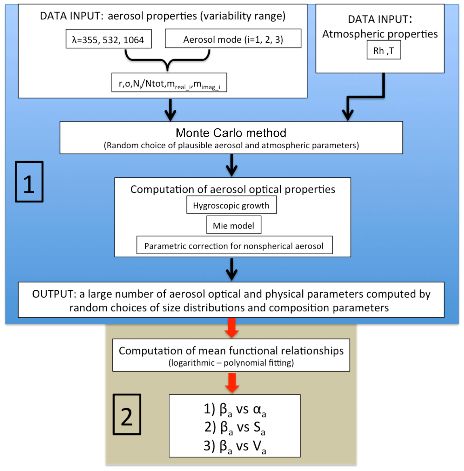
Figure 1Schematic of the two-step model structure developed to obtain, as a result, functional relationships between the aerosol backscatter (βa) and the aerosol extinction, surface area, and volume (αa, Sa, and Va, respectively).
-
Generate a large set (here 20 000) of aerosol optical and physical properties by randomly varying, within appropriate ranges, the microphysical parameters describing the aerosol size distribution and composition (blue box in Fig. 1).
-
Based on results at point 1, determine mean functional relationships linking such key variables (grey box in Fig. 1).
The following section describes rationale and setup of the first step; the second step is thoroughly discussed in Sect. 3.
2.1 Selection of the aerosol microphysical parameters
As anticipated, an average continental aerosol type (i.e., describing clean to moderately polluted continental conditions; e.g., Hess et al., 1998) was targeted in this study, this being the aerosol type expected to dominate over Europe. Based on a scheme originally proposed by d'Almeida et al. (1991) and a large set of observational evidence (e.g., Van Dingenen et al., 2004), in this work the size distribution is described as an external mixture of three size modes. These are (in order of increasing size range) (1) a first ultrafine mode; (2) a second fine mode, mainly composed of water-soluble particles; and (3) a third mode of coarse particles.
A three-mode lognormal size distribution described by Eq. (1) is employed for this purpose:
In Eq. (1), ri, σi, and Ni are respectively the modal radius, the width, and the particle number density of the ith aerosol mode (i= 1, 2, 3). At each computation, ri and σi are randomly chosen within a relevant variability range. Values of Ni are conversely obtained by firstly randomly choosing the total number of particles, Ntot, to be included in the whole size distribution () and then by applying specific rules for the number mixing ratio, , of each component to this total. To reproduce clean to moderately polluted continental conditions, the value of Ntot is made variable between 500 and cm−3 (e.g., Hess et al., 1998; Van Dingenen et al., 2004). As the result of different sources and processes, the three modes are also assumed to have a different composition, which impacts the optical computations through the relevant particle refractive index (mi), with both its real and imaginary components (. The Mie theory for spherical particles of radius ri and refractive index mi is then used to compute the extinction and backscatter coefficients (see below).
Table 1Aerosol parameter values as reported in literature for continental-type aerosols.
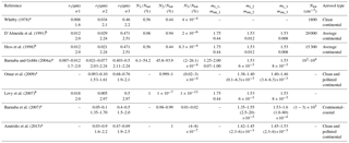
aThe refractive index is at λ=532 nm. bThe refractive index is at λ=550 nm.
Table 2Variability ranges used in this study. Values refer to ground and dry conditions (see text for details).
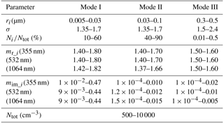
A description of the assumptions made for each mode and relevant parameter, mostly based on literature data (Table 1), is given hereafter; the summary of the relevant variability chosen for each parameter is provided in Table 2.
-
First mode. This ultrafine mode is the one more directly simulating fresh anthropogenic emissions. The number mixing ratio xi=1 () of this mode is let variable between 10 % (rural conditions; Van Dingenen et al., 2004) and 60 % (more polluted conditions; Hess et al., 1998). The variability in its modal radius (r1=0.005–0.03 µm) is chosen to include nucleation-mode particles to Aitken-mode particles. To take into account the wide variability in species within this ultrafine mode, from non-absorbing (e.g., inorganic particles) to highly absorbing materials (e.g., black carbon), wide ranges of variability have been set for its refractive indexes (at λ=355 nm: mr_1 in the range 1.40—1.8, and mim_1 in the range 0.01–0.47; see Table 2 for the corresponding values at λ=532 and 1064 nm).
-
Second mode. The second aerosol mode accounts for 40 %–90 % of Ntot, with (dry) r2 between 0.03 and 0.1 µm. Its composition (mr_2, and mim_2) is also made highly variable so as to include water-soluble inorganic and organic particles (Hess et al., 1998; BG04a; Dinar et al., 2008). In this case, at λ=355 nm, mr_2 is in the range 1.40–1.7 and mim_2 is in the range 0.0001–0.01 (Table 2).
-
Third mode. This coarser aerosol mode (modal radius r3 in the range 0.3–0.5 µm) is mainly intended to account for soil-derived (dust-like) particles that are a primary continental emission. A quite narrow variability is thus fixed for its mr_3 and mim_3 values (1.5–1.6 and 0.0001–0.02, respectively, at 355 nm). The relevant number mixing ratio x3 (N3∕Ntot) is set as variable between 0.01 % and 0.5 %, with this mode contributing mostly to the total aerosol volume (thus mass) rather than to the total number of particles.
As mentioned, refractive indexes were also made wavelength dependent, as this feature is also typically observed as linked to the different particle composition. In particular, for the second mode (water-soluble particles) we include an increase with the wavelength of the upper boundary values of mim_2 and a decrease in mr_2 at λ=1064 nm (d'Almeida et al., 1991). For the (dust-like) third-mode particles, the upper boundary values of mim_3 are set to decrease with increasing wavelengths (Gasteiger et al., 2011; Wagner et al., 2012).
For convenience, the aerosol parameter boundaries summarized in Table 2 refer to dry particles and to ground level. However, the effect of a variable relative humidity (RH), its variability with altitude, and the generally observed decrease in particle number with altitude is also considered in the model. More specifically, the number of particles in each mode, Ni, and RH are both made altitude dependent through the following equations (Patterson et al., 1980; BG01):
The altitude z is variable here between 0 and 5 km. Ni(0) and Hi in Eq. (2) are the number of particles at the ground and the scale height for each mode, respectively.
To describe the altitude effect, in Eq. (2) an exponential decrease with height of the particle number density is assumed. To rescale the particle number density of the different modes, is set equal to 5.5 km (Barnaba et al., 2007) while Hi=3 (coarse particles) is set to 0.8 km (Barnaba et al., 2007). In Eq. (3), the additional term (1 + dRH) allows a further variability with respect to the mean RH(z) profile assumed; here dRH is randomly chosen between −60 and +60. Values of RH greater than 95 % are discarded to avoid divergence.
Additionally, while the first and third modes are assumed to be water insoluble, the second mode (i=2) is fully hygroscopic. Aerosol humidification is thus considered to act on both particle size and refractive indices of the second aerosol mode (e.g., BG01) as
In Eqs. (4) and (5), r2_RH and m2_RH are the RH-corrected modal radius and refractive index for the second mode, respectively; r2_0 and m2_0 are the particle dry modal radius and refractive index, respectively; mw is the water refractive index (assumed to be equal to , and , at 355, 532, and 1064 nm, respectively).
Finally, following Barnaba et al. (2007), an increase in the width of the size distribution with altitude (Eq. 6) has been introduced for the first and second aerosol modes:
In fact, Barnaba et al. (2007) showed that this was necessary to better reproduce the observed decrease in the lidar ratio (LR) with altitude, and is likely related to a broadening of the particle size distribution with aging.
Once the value of each microphysical parameter is randomly selected within its relevant variability range, and once corrections are applied following Eqs. (2)–(6), each resulting aerosol size- and composition-resolved distribution is used to compute the aerosol Sa and Va, as well as to feed a Mie code (assumption of spherical particles; Bohren and Huffman, 1983) to compute βa and αa (BG01; see also Fig. 1). Overall, the equations used are as follows.
Here Qbsc (ri, λ, mi) and Qext (ri, λ, mi) are, respectively, the backscatter and the extinction efficiencies. As mentioned, the optical computations are made at the three different wavelengths: 355, 532, and 1064 nm (i.e., those of Nd:YAG laser harmonics, the most common wavelengths used by ground-based and spaceborne aerosol lidars).
Since in our simulations the third aerosol mode is intended to represent dust-like particles, an empirical correction for non-sphericity is also applied to the Mie-derived optical properties of this mode. This procedure is based on BG01, which uses the results of Mishchenko et al. (1997) obtained for surface-equivalent mixtures of prolate and oblate spheroids.
2.2 Model simulation results
In Fig. 2 we show the results of 20 000 simulations of continental aerosol optical and physical properties derived randomly, varying the relevant aerosol size distributions and compositions as described in the previous section. In particular, the results for αa, Sa, and Va are shown as a function of βa in Fig. 2a, b, c (blue crosses) referring to λ=1064 nm. For each variable (A), the average value per bin of βa and relevant standard deviations (〈A〉±dA) are shown as red dots and vertical bars, respectively. Note that 10 equally spaced bins per decade of β have been considered and that 〈A〉±dA values are only shown for bins containing at least 1 % of the total number of pairs. Corresponding relative errors (dA∕〈A〉) are depicted in Fig. 2d, e, f. Some sensitivity tests of these model outputs to the variability in the input microphysical parameters employed are provided in Appendix A.

Figure 2Scatter plots of (a) αa (km−1), (b) Sa (cm2 cm−3), and (c) Va (cm3 cm−3) vs. backscatter βa (km−1 sr−1) and relevant relative errors (d, e, f) as derived from 20 000 model computations (blue points) at λ=1064 nm. Red dots and error bars are the average values per decade of β and their standard deviations; green lines are the seventh-order polynomial fit curve of the 20 000 points.
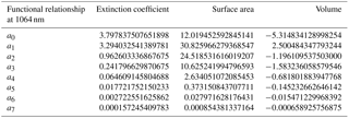
Based on these results, at step two of the procedure (see scheme in Fig. 1), we derive aerosol-specific mean relationships linking aerosol extinction, surface area, and volume (αa, Sa and Va) to its backscatter (βa). For this purpose, we used a seventh-order polynomial fit in log–log coordinates. The choice of a seventh-order polynomial fit was made for homogeneity with BG01 and BG04a. These relationships are shown as green lines in Fig. 2a, b, c while the relevant fit parameters are reported in Table 3 referring to λ=1064 nm (fit parameters related to computations at λ=355 and 532 nm are given in Table B1 and Table B2, Appendix B).
Table 3Parameters of the seventh-order polynomial fits () for λ=1064 nm, with x=log(βa) (in km−1 sr−1) and in km−1, cm2 cm−3, and cm3 cm−3, respectively.
The red vertical bars of Fig. 2 also highlight the ranges of αa, Sa, and Va, which are statistically significant, i.e., those in which, at λ=1064 nm, the model provides at least 1 % of the total points per corresponding bin of βa. These are 10−4–10−1 km−1, 10−7–10−5 cm2 cm−3, and 10−13–10−10 cm3 cm−3, for αa, Sa, and Va, respectively, corresponding to the backscatter range km−1 sr−1. In terms of aerosol property variability, the relative errors associated with αa and Va show almost no dependence on βa, with values between 30 % and 40 %. Conversely, the modeled aerosol surface area exhibits a larger dispersion, with relative error values spanning the range 40 %–70 %, and decreasing as βa increases.
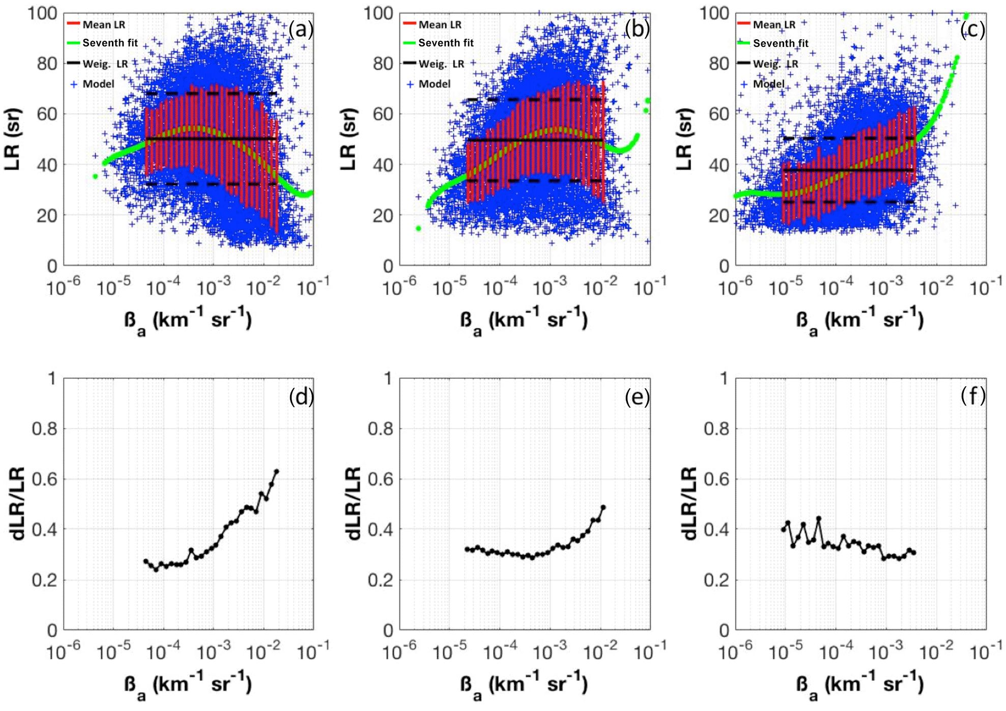
Figure 3(a, b, c) Scatter plots of LR (sr) versus βa (km−1 sr−1) at (a) 355 nm, (b) 532 nm, and (c) 1064 nm (blue points). The seventh-order polynomial fit curve (green lines) and the average values per decade of β together with their standard deviations (red points and red vertical bars, respectively) are also reported. Horizontal black lines are mean values of the weighted-LR and ±1 SD (solid and dashed lines, respectively). (d, e, f) Relative errors associated with the model-derived LR at (d) 355 nm, (e) 532 nm, and (f) 1064 nm.
A key parameter for the inversion of lidar signals is the LR, i.e., the ratio between αa and βa (Ansmann et al., 1992). In Fig. 3 we thus show the results of our simulations in terms of LR vs. βa at the three λ (355, 532, and 1064 nm, Fig. 3a, b, c, respectively) and relevant dLR ∕ LR values (Fig. 3d, e, f, respectively). The color code is the same as in Fig. 2. Additional horizontal black lines have been inserted representing values (solid central lines) of the weighted-LR ± 1 standard deviation (dotted side lines), i.e., the LR weighted by the number of simulated points in each considered backscatter bin. The weighted-LR values derived at 355, 532, and 1064 nm are 50.1±17.9, 49.6±16.0, and 37.7±12.6 sr, respectively. Figure 3 also allows showing that the statistically significant regions of simulated backscatter values shift towards smaller values with increasing λ (e.g., at λ=355, the βa extending region is – km−1 sr−1, whereas, at 532 nm, it ranges between and km−1 sr−1). Furthermore, Fig. 3 reveals a quite different shape of the LR vs. βa functional relationships (green curves) at different wavelengths. At 355 and 532 nm the curve is concave, with quite similar LR maxima of the fitting curve (54.3 and 53.8 sr at approximately and km−1 sr−1, respectively). At 1064 nm the curve is conversely monotonic, with a flex point at βa=3– km−1 sr−1. A larger data dispersion also characterizes the results at λ=355 and 532 nm (LR values from 10 to 90 sr) in comparison to λ=1064 nm (LR in the range 18–80 sr, except for a minor number of outliers). This translates into different LR relative errors at UV, VIS, and infrared (IR) wavelengths. At 1064, dLR∕LR slightly decreases for increasing backscatter, with values of around 35 %. At the shorter wavelengths, dLR∕LR increases as a function of βa, with a large (>40 %) relative error for values of km−1 sr−1.
Table 4Mean weighted LR at 355, 532, and 532 nm derived in this work and comparison to the corresponding aerosol subtypes (clean continental, CC, and polluted continental, PC) from relevant literature.
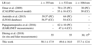
a Derived using the extinction-related and backscatter-related Ångström exponents given by Amiridis et al. (2015). b See the explanation in the text for the two different values.
To insert our results into a more general context, we compared the derived, model-based weighted-LR values to some LR data reported in the literature (Table 4). In particular, we selected some of the works using the aerosol model developed to invert the CALIPSO lidar data. For example, Omar et al. (2009) consider six different aerosol subtypes: clean continental (CC), clean marine (CM), dust (D), polluted continental (PC), polluted dust (PD), and smoke (S). Our model-derived LR at 532 nm falls in the middle of the range (35–70 sr) fixed by the CALIPSO CC and PC aerosol classes. The work by Papaggianopoulos et al. (2016), in which the LR values are adjusted according to EARLINET observations, reports a LR range at 532 nm of 47–62 sr. At the same wavelength, the aerosol range defined by the LIVAS climatology (LIdar climatology of Vertical Aerosol Structure for space-based lidar simulation studies; Amiridis et al., 2015) is 54–64 sr. In both cases, our model seems to be closer to the LR values of the CC aerosol type, which is compatible with our intention to simulate the clean to moderately polluted continental aerosol type. At 532 nm, our LR value is also reasonably in between the CC and PC LR values derived by Omar et al. (2009), but again closer to the CC LR value. The very small decrease in LR values between 532 and 355 nm estimated by LIVAS for the CC aerosol is also consistent with our results. Similarly, our model predicts a lower mean LR in the near IR with respect to the green, in agreement with results of Amiridis et al. (2015) in CC conditions and not with those in polluted conditions. Table 4 also includes the continental aerosol LR values estimated in the work of Düsing et al. (2018) through comparison between airborne in situ and ground-based lidar measurements. Our model is in good agreement with their LR values at 355 and 532 nm. At 1064 nm, the algorithm developed by Düsing et al. (2018) provided a value of LR of around 15 sr. Conversely, in the same study the authors found that, rather, a value of LR = 30 sr gives the better agreement between their Mie and lidar-based αa, this value being closer to our model-derived one at 1064 nm (LR = 37.7). The difference between these two values is explained by the authors to be probably due to the estimation of the aerosol particle number size distribution, a critical parameter for a reliable modeling of aerosol particle backscattering.
Table 5Extinction-to-volume conversion factors, (and corresponding mass-to-extinction efficiency values, MEE ), computed employing ρa=2 g cm−3) of continental particles as derived from our model at different wavelengths.
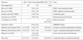
As a last added value of the outcome from our model-based results, we derive here and provide in Table 5 extinction-to-volume conversion factors, (e.g., Ansmann et al., 2011) at three different wavelengths (355, 532, 1064 nm) and compare these to similar outcomes from other studies. To our knowledge, values of continental particles cv at three wavelengths are only available in Mamouri and Ansmann (2016). Note that cv is also proportional, through the particle density ρa, to the inverse of the so-called mass-to-extinction efficiency (MEE, i.e., , a parameter important in several aerosol-related applications (e.g., the estimation of PM from satellite AOT or in modules of global circulation and chemical transport models to compute aerosol radiative forcing effects; Hand and Malm, 2007). For convenience, model-derived MEE values are also included in Table 5.
In this section, we evaluate the capability of the model results to reproduce “real” aerosol conditions and explore the potential of the proposed model-based ALC inversion in producing quantitative geophysical information.
-
In Sect. 3.1 we compare our simulations to real observations of independent backscatter and extinction coefficients made by different EARLINET Raman lidars (Bösenberg et al., 2001; Pappalardo et al., 2014).
-
In Sect. 3.2, our model results are used to invert measurements acquired by some ALC systems operating within ALICEnet, which networks several ALC systems (Nimbus CHM 15k by Lufft) located across Italy and run by Italian research institutions and environmental agencies. Here we use data from some of these systems to derive the aerosol optical and physical properties (e.g., the AOT and the aerosol volume and mass).
3.1 Comparison of the modeled aerosol optical properties to EARLINET measurements
As mentioned, EARLINET Raman stations perform coordinated measurements 2 days per week following a schedule established in 2000 (Bösenberg et al., 2003). Overall, the EARLINET database includes the following categories: climatology, CALIPSO, Saharan dust, volcanic eruptions, diurnal cycles, cirrus, and others (forest fires, photo smog, rural or urban, and stratosphere). To be comparable to our results, we used EARLINET βa and αa coefficients at 355 and 532 nm within the quality-assured (QA) climatology category (Pappalardo et al., 2014). However, note that additional data filtering was necessary to screen out residual, likely unreliable values within this QA climatology category. In particular, we only selected those EARLINET QA data further satisfying the following criteria:
-
βa and αa coefficients evaluated independently, i.e., only obtained using the Raman method (Ansmann et al., 1992);
-
βa and αa>0;
-
LR < 100;
-
relative errors on βa and αa<30 %.
Then, we selected those sites in Europe expected to be mostly impacted by continental aerosols and having the largest datasets (e.g., at least 100 points) at 355 and 532 nm. Overall, five sites satisfied these conditions (Table 6), namely Madrid (Spain), Potenza and Lecce (Italy), and Leipzig and Hamburg (Germany). Finally, being interested in continental conditions here, we filtered out those measurement dates affected by desert dust at the measuring sites, i.e., we removed from our “model–measurement comparison dataset” all the dates within the EARLINET climatology category also belonging to the EARLINET Saharan dust category.
Table 6Main characteristics of the dataset of the EARLINET continental sites considered in this study. The listed dataset refers to the data downloaded from the EARLINET site (last access on the 11 January 2018). NA – not available.
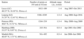
Figure 4 depicts the results of the model–measurement comparison at the sites fulfilling our requirements in terms of LR vs. βa at λ=355 nm (the corresponding results at λ=532 nm, including Madrid in place of Hamburg, are given in Appendix C, Fig. C1). The colored area represents the model-simulated data range, while the color code indicates the absolute number of simulated values (i.e., counts) in each βa–LR pair. The EARLINET-measured values are reported as open black circles. Note that, since the model simulations are performed over an altitude range of 0–5 km (see Sect. 2.1), only those simulations corresponding to the altitude range (Δz) covered by the measurements at each EARLINET station were taken into account here. Figure 4 shows that the model results encompass the measured LR vs. βa data well, with a few measurements outside the modeled range (most of the exceptions are found for Potenza). Statistically, the highest number density of simulated data fits the observations well, with the exception of Hamburg (Fig. 4a), which has the lowest number of measured data (it is not an EARLINET station any longer; see Table 6).
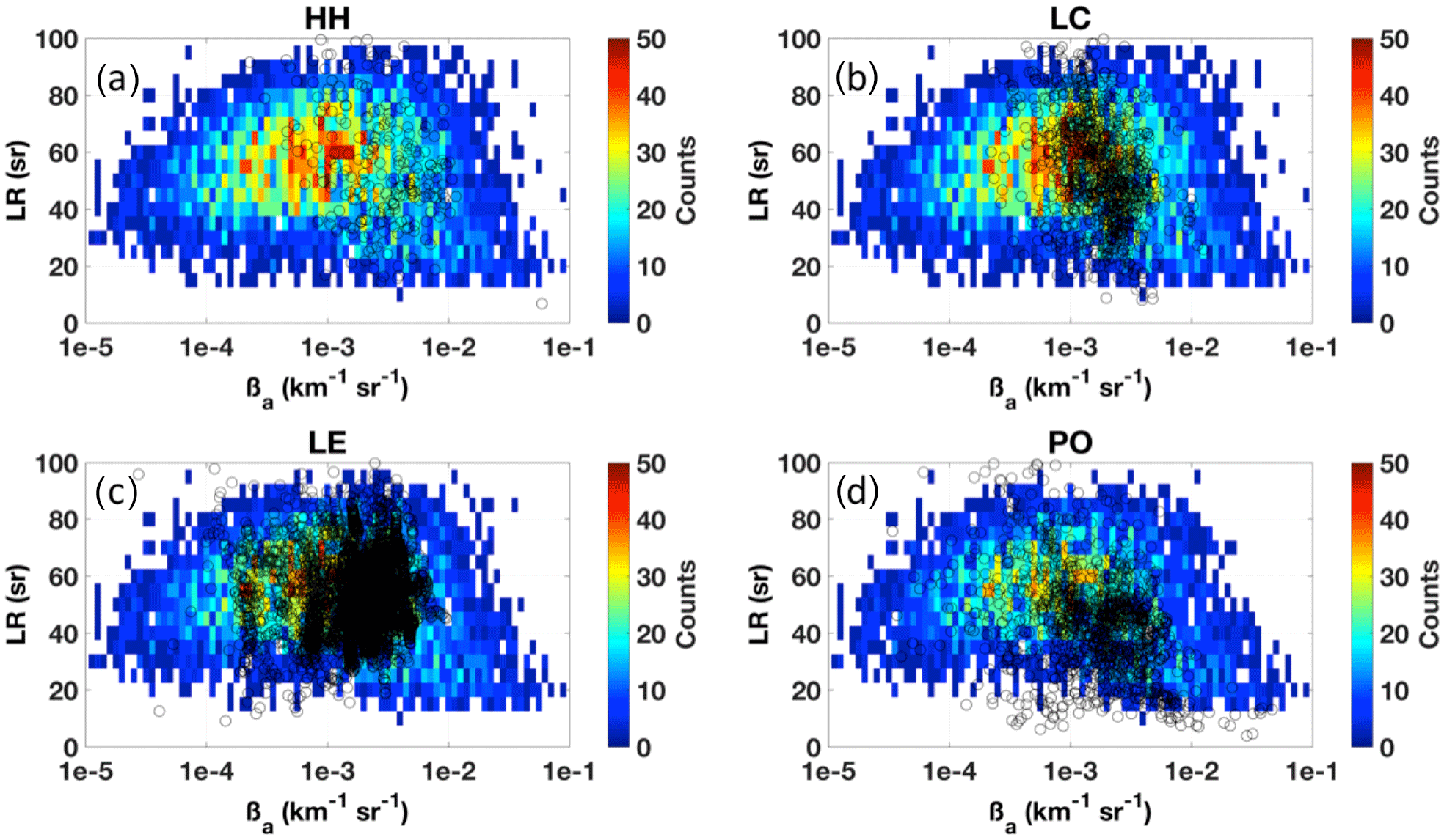
Figure 4Scatter plots of LR (sr) versus βa (km−1 sr−1) at 355 nm as simulated by our model (colored region) and measured by EARLINET lidars (open black circles) in Hamburg (Germany) (a), Lecce (Italy) (b), Leipzig (Germany) (c), and Potenza (Italy) (d). The colored area is the region of simulated values, the color code indicating the number of simulated values in each βa–LR pair (see legend). In particular, the color 2-D histogram is computed using a semilogarithmic box consisting of 10 equally spaced bins per decade of βa on the x axis and five spaced LR values on the y axis.
Table 7Mean LR discrepancies between our model results and EARLINET measurements and weighted LR at 355 and 532 nm for the considered EARLINET stations. LC: Lecce; LE: Leipzig; PO: Potenza; HH: Hamburg; MA: Madrid.
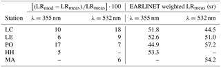
In Fig. 5 the previous results at λ=355 nm are converted in terms of mean LR per bin of βa for both model (blue) and observations (red, again, only βa bins containing at least 1 % of the total modeled data were considered). This view shows that there is a general good agreement between the modeled and the measured LR values, and in their variation with βa. Some major deviations are found for Potenza and are further discussed in the following. The model–measurement agreement shown in Fig. 5 was evaluated in quantitative terms by computing mean LR relative differences at both λ=355 and 532 nm; i.e., we derived ([(LR) values, for which LRmod and LRmeas are the LR values computed by the model and derived using lidar measurements, respectively. These values are reported in Table 7 for each considered EARLINET station, together with the measurement-based mean LR in each observational site (computed weighting the number of observations per βa-spaced bins).
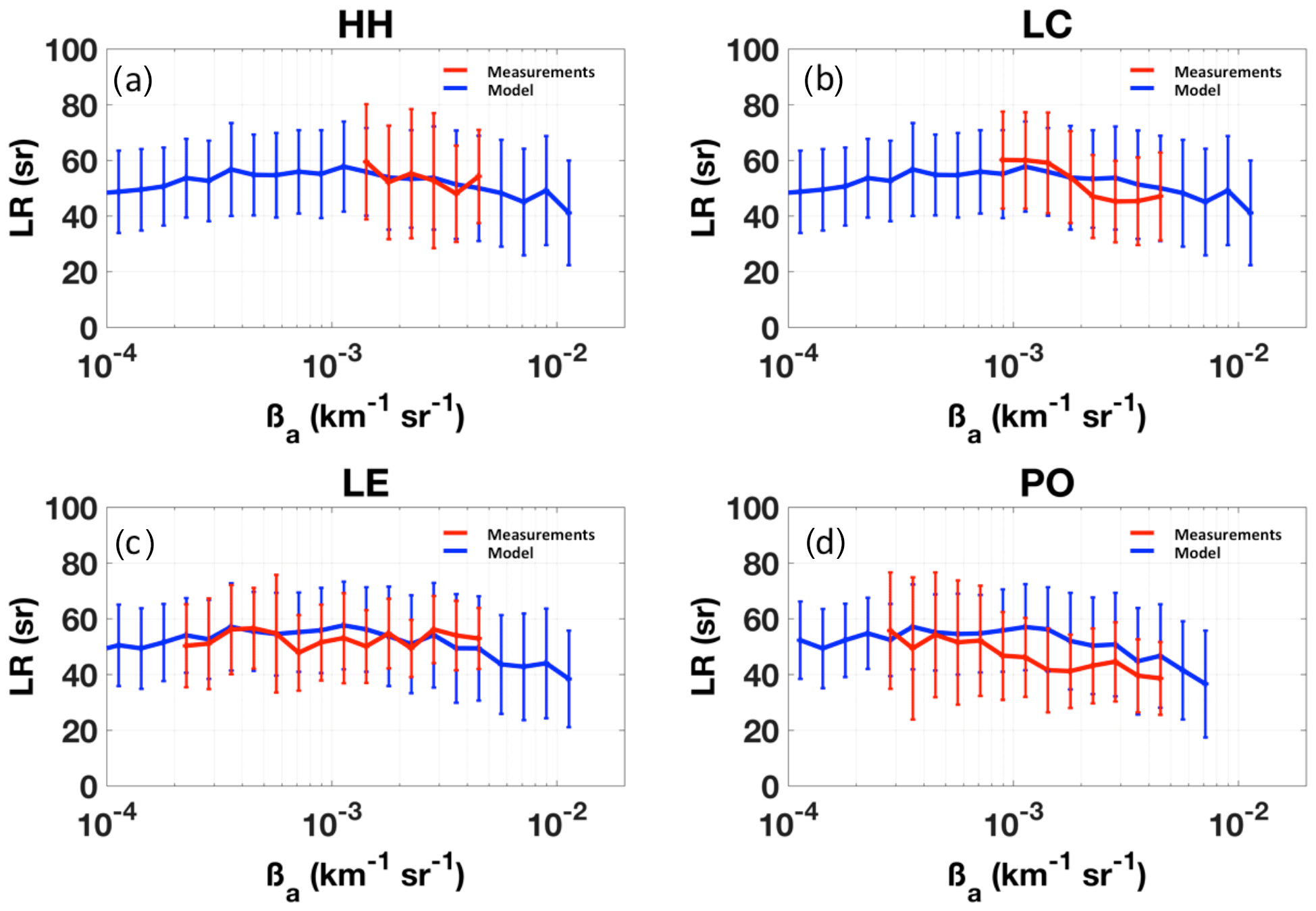
Figure 5Model-simulated (blue) and lidar-measured (red) LR vs. βa mean curves at 355 nm calculated per 10 equally spaced bins per decade of βa at the (a) Hamburg (HH), (b) Lecce (LC), (c) Leipzig (LE), and (d) Potenza (PO) EARLINET lidar stations. Vertical bars are the associated standard deviations.
Results in Fig. 5 and Table 7 also give some hints on the capability of the aerosol type assumed (and its admitted ranges of variability) to reproduce real continental aerosol conditions at different sites across Europe. In fact, the four continental sites selected with our criteria are still expected to be partially impacted by different aerosol types.
-
A good agreement between the model and the observations in terms of LR mean values is found for Hamburg (Fig. 5a), with mean LR differences of the order of 5 % (Table 7). Still, the measured LR values have a high variability and their distribution is positioned towards high values of βa ( to km−1 sr−1). This could be due to the presence of different aerosol types as slightly polluted marine and polluted aerosol (Matthias and Bösenberg, 2002).
-
A good accord for Leipzig (Fig. 5c) also indicates that this site is mostly dominated by pure continental particles. In fact, the distribution of observed LR points in Fig. 4, which covers βa values ranging from to km−1 sr−1, is well centered to the modeled simulations' highest density (counts >40). Table 7 shows that at both wavelengths mean discrepancies with LR measurements stay well below 10 %.
The highest differences in Fig. 5 are found at some southern Europe EARLINET sites.
-
In Lecce (Fig. 5b), the best agreement between model and observations is found for the lowest values of βa (between and km−1 sr−1; see Table 7). Also, the increase from 10 % to 18 % in the discrepancies at 355 and 532 nm indicates some model problems in correctly reproducing the spectral variability in the optical properties, suggesting some mismatch between modeled and real aerosol sizes at this site (see discussion below).
-
In Potenza (Fig. 5d), a significant difference between the mean LR curves emerges for βa values km−1 sr−1 , with observed LR values lower than those simulated here.
These discrepancies could be due to the influence of marine aerosols at both stations (De Tomasi et al., 2006; Mona et al., 2006; Madonna et al., 2011), which is expected to produce lower LR values for high values of βa (e.g., BG01). In fact, Madrid shows better performances, with dLR∕LR values comparable to those in Leipzig.
To provide some insight into the reasons of the model–measurement differences at the Lecce and Potenza sites, some specific model sensitivity tests have been performed and are reported in Appendix D. In particular, for Lecce, we found that better agreement between the observed and simulated LR vs. βa behavior at 355 nm is obtained by reducing the variability range of Ntot (from 500–10 000 to 500–5000 cm−3 at ground). This indicates that Lecce is likely affected by cleaner continental aerosol-type conditions. The sensitivity simulations performed for understanding the mismatches with Potenza measurements show that an extension of the variability range of the coarse-mode radius is needed to reproduce the observed decrease in LR for increasing backscatter (Fig. 5d). This suggests a contribution of coarse particles larger than that assumed (Appendix D). This is compatible with the suspect of marine air contamination, although at this stage we are not able to exclude additional contamination of coarser particles of soil origin.
Overall, mean LR differences between our average continental model and data at selected continental sites in Europe remain lower than 20 % (Table 7), indicating the model reasonably reproduces the clean-to-moderately polluted continental aerosol conditions we intended to simulate well.
3.2 Application of model results to Nimbus CHM 15k ALC measurements
To test and validate the model-based inversion methodology, we used the derived functional relationships (Sect. 2.2) to invert and analyze the measurements of some ALICEnet ALCs (Lufft Nimbus CHM 15k systems). These instruments are biaxial ceilometers that emit laser pulses at 1064 nm (Nd:YAG laser, class M1) with a typical pulse energy of 8 µJ and a pulse repetition rate of about 6500 Hz. The instruments have a specified range of 15 km and fully overlap at around 1500 m (Heese et al., 2010). The manufacturer provides the overlap correction functions (O(z)) for each system. As shown recently by Wiegner and Geiß (2012) and Wiegner et al. (2014), a promising strategy to retrieve the aerosol backscatter coefficient from ALC measurement is adopting the forward solution of the Klett inversion algorithm (Klett, 1985). This solution requires a known calibration constant of the system (i.e., absolute calibration, cL) and an assumption of the LR. The advantage with respect to the backward solution is that calibration is not affected by the low SNR in the upper troposphere and it is needed occasionally. Furthermore, starting close to the surface, the data retrieval allows us to resolve aerosol layers in the boundary layer even if their optical depth is high. The forward solution of the Klett inversion algorithm is thus adopted here. For convenience, we report here the equations used within our procedure to obtain βa from ALC measurements, which are also described in Wiegner and Geiß (2012, Eqs. 1–3):
with
and
Here, βm and αm are the molecular backscatter and extinction coefficients calculated from climatological monthly air density profiles and z2P(z) is the ALC range-corrected (z) signal (P) (also referred to as RCS), which are the raw data obtained by the considered ALCs. As anticipated, knowledge of the calibration constant cL is needed to solve Eq. (13) (and thus 11, forward solution). In our analysis of ALC daily records, the constant cL has been obtained using the “backward approach” (Rayleigh calibration) applied to nighttime cloud-free ALC signals averaged over 1 or 2 h at 75 m height resolution. This allows for using the best cL retrieval (that is the nighttime lowest noise one) in the forward solution of the lidar equation, which guarantees operating over the best signal-to-noise range of the ALC signal.
3.2.1 Model-based retrieval of aerosol optical properties
Operatively, inversion of the aerosol properties, αa(z) and βa(z), is performed using an iterative technique since we need to correct the backscatter signal at each altitude z for extinction losses. The iterative procedure is stopped when convergence in the integrated aerosol backscatter (IAB ) is reached (e.g., BG01). At each step, aerosol extinction is derived using the functional relationship αa=αa (βa) of Table 3.
Figure 6Time–height cross section of the aerosol extinction coefficients αa (km−1), as derived at 1064 nm on 26 June 2016 by the ALICEnet ALC of Saint-Christophe in the Aosta Valley (northern Italy). The orange circle points and the pink line are the AOT values (right y axis) measured by a colocated POM-02L radiometer and estimated from the ALC following our approach.
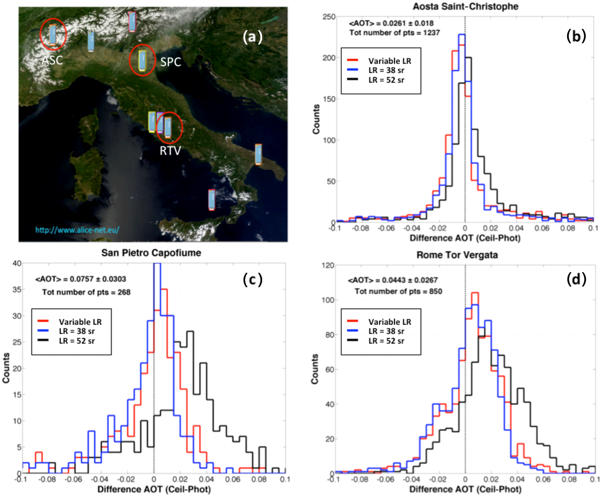
Figure 7(a) Geographical map of the ALC network ALICEnet. The red circles highlight the selected sites for this study: Saint-Christophe in the Aosta Valley (ASC), San Pietro Capofiume (SPC), and Rome Tor Vergata (ASC). (b)–(d) Histograms of the differences between the hourly-mean coincident AOTs at 1064 nm as derived by ALCs and measured by photometers at ASC, SPC, and RTV, respectively. The different colors (red, blue, and black) depict the different inversion schemes: model-based inversion scheme, LR = 38 sr and LR = 52 sr. In each panel the values of the average measured AOT (and its associated standard deviation) and of the number of considered pairs are also reported.
An example of the outcome of this retrieval methodology is depicted in Fig. 6. It shows the time–height (24 h, 0–6 km) contour plot of αa retrieved at 1064 nm during a whole day of measurements (26 June 2016) performed by the ALICEnet system of Saint-Christophe in the Aosta Valley (ASC, 45.7∘ N, 7.4∘ E 560 m a.s.l., northern Italy; Fig. 7a). Time and altitude resolutions are 1 min and 15 m, respectively. Note that ALC data are cloud-screened using the cloud mask of the Lufft firmware.
The AOT is obtained by vertically integrating the ALC-derived αa(z) from the surface up to a fixed height zAOT, above which the aerosol contribution is assumed to be negligible. In Fig. 6, the ALC-derived AOT values at 1064 nm (pink curve, with a temporal resolution of 5 min) are superimposed on the extinction contour. Reference AOT values from a colocated sun–sky radiometer (a Prede POM-02 system) are shown by orange circles. These were extrapolated at 1064 nm from the instrument 1020 nm channel using the Ångström exponent derived fitting AOT values at all the radiometer wavelengths. This example illustrates the very good performances of our model-assisted inversion scheme and the capability of this approach to extend the (daylight-only) radiometer observations to nighttime.
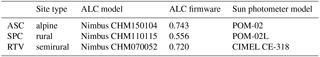
Table 8Main characteristics of the ALC and colocated sun–sky radiometer equipment located at the considered ALICEnet sites.
To evaluate the performances of our model-assisted retrieval of αa(z) over a more statistically significant dataset, the same approach illustrated in Fig. 6 was applied to a longer record at the ASC site, plus Nimbus CHM-15k ALC datasets from two additional ALICEnet sites: San Pietro Capofiume (SPC, 44∘39 N, 11∘37 E, 10 m a.s.l.) and Rome Tor Vergata (RTV, 41.88∘ N, 12.68∘ E, 100 m a.s.l.). The location of the instruments is shown in Fig. 7a (red circles), while some information on system types and site characteristics is given in Table 8. The data analyzed here were collected during the following periods: April 2015–June 2017, June 2012–June 2013, and February 2014–September 2015 for ASC, SPC, and RTV, respectively.
At those sites, reference AOTs were collected by three colocated sun–sky radiometers, namely using two SKYNET Prede sun–sky radiometers at ASC and SPC (POM-02L and POM-02, respectively, http://www.euroskyrad.net/, last access: 29 October 2018) and an AERONET (AErosol Robotic Networ; Holben et al., 1998) Cimel CE 318-2 instrument operational at RTV (https://aeronet.gsfc.nasa.gov, last access: 29 October 2018, Rome Tor Vergata station, data level 2.0). Only AOT values between 0.01 and 0.2 at 1064 nm were considered. This range allows for excluding the data points with a 1064 nm AOT lower than the sun photometer expected accuracy (dAOT = 0.01) and those for which we found aerosol extinction to cause significant deterioration of our ALC signal. Overall a total of 1237, 268, and 850 AOT pairs were analyzed at ASC, SPC, and RTV, respectively.
Also note that, although CHM-15k data are already corrected for the O(z) function provided by the manufacturer, the variation in the ALC internal temperature was shown to lead to O(z) differences of up to 45 % in the first 300 m above ground (Hervo et al., 2016). For this reason, in our analyses the lowest valid altitude of the CHM-15k for both the SPC and RTV systems was fixed to be about 400 m. A linear fit of the first two valid ALC points is then used to extrapolate αa(z) down to the ground (z0). Conversely, due to the optimal characterization down to the ground of O(z) provided by Lufft for the CHM-15k system installed at ASC, values at z0 at this site are not those extrapolated but actually those measured. The maximum altitude of aerosol extinction vertical integration to derive the AOT, zAOT, was selected as the first height above 4000 m at which the range-corrected signal (RCS) has a SNR < 1.
Table 9Results of the comparison between the AOT measured by sun photometers and the one derived by ALCs (model-based and fixed-LR inversion schemes) at three ALICEnet stations. Mean differences (expressed in terms of , (module), , and ) are reported with their standard deviations.
Results of the long-term AOT comparison are summarized in Fig. 7 and Table 9. For each site under investigation, Fig. 7 shows the histograms of the AOT differences between the hourly-mean coincident AOTs as derived by the ALCs and measured by the sun photometers (red curve; corresponding AOT vs. AOT scatter plots at the three considered sites are given in Appendix E). To evaluate the advantage of our approach with respect to more standard lidar inversions, we also computed AOT differences using two fixed-LR values. In particular, we used LR = 52 sr (i.e., the value suggested by the E-PROFILE network, black lines) and LR = 38 sr (i.e., the weighted mean LR value derived from our model; see Sect. 3, blue lines). Figure 7 shows that the best agreement is found at ASC. The distribution of AOT difference has a maximum of around 0 for each of the three inversion schemes, with very low dispersion. The full width at half maximum, FWHM, is in fact around 0.015, and approximately 55 % of the data are included in the interval −0.01–0.01, which is even within the expected error of photometric measurement. For SPC and RTV, the red and blue histograms are peaked around 0, whereas the black ones are shifted, with maxima around 0.01–0.02 and 0.02–0.03 for SPC and RTV, respectively. These two sites have higher dispersion (FWHM = 0.03), and approximately 30 % of the data are included in the interval −0.01–0.01 for the red and blue histograms at both sites, which is probably due to the different aerosol load affecting the different ALICEnet stations. As pointed out by the low value of the average AOT computed at ASC for the analyzed dataset (〈AOT〉=0.027), low pollution levels generally characterize this site, with some exceptions due to wind-driven aerosol transport from the nearby Po Valley (Diémoz et al., 2014, 2018a, b). Conversely, RTV (〈AOT〉=0.044) and especially SPC in the Po Valley (〈AOT〉=0.076) are characterized by higher aerosol content and pollution levels, which explain the larger histogram dispersions. Note that the high frequency of fog events in winter markedly reduces the number of analyzed AOT pairs at the SPC site, while some desert-dust-affected days at both SPC (e.g., Bucci et al., 2018) and RTV (e.g., Barnaba et al., 2017) were removed from our datasets (no desert-dust-affected dates in ASC).
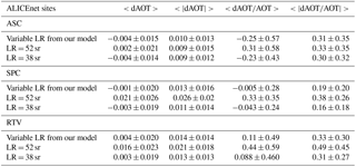
Table 9 summarizes the long-term performances of the model-based procedure in deriving quantitative AOT from the ALC systems at the three investigated sites. It includes values of the average differences between the ALC-derived and sun-photometer-measured AOT (both bias 〈dAOT〉, and absolute difference , with associated standard deviations) obtained using both the proposed model-based approach and the fixed-LR inversions. For the SPC and RTV sites, these numbers show that the best ALC–photometer accordance is reached when employing either the model-based or the fixed-LR = 38 sr inversion scheme. In fact, these two approaches have similar performances in terms of mean dAOT values (, 0.013 and 0.013, 0.014 for SPC and RTV, respectively), mean percent error (, 0.19 and 0.31, 0.33), and a very low mean relative bias (, 0.005 and 0.088, 0.11). Conversely, the fixed-LR = 52 sr retrieval produces an overestimation of AOT in both SPC and RTV ( and 0.44), with larger discrepancies between retrieved and observed AOTs ( and 0.026, and 0.49). For the ASC site, due to the low aerosol content, the differences among the inversion schemes are almost negligible.
Overall, for the three sites, the statistics over the long-term datasets employed showed good results of the model-based approach with similar behavior of the retrievals with a fixed LR of 38 sr, while a fixed LR value of 52 sr produces an overestimation of the AOT at SPC and RTV. As different sites have different (and not known a priori) characteristic LR values, these results highlight the potential of the model-based approach to derive quite accurate βa and αa coefficients without the need to choose and fix an arbitrary LR value.
3.2.2 Model-based retrieval of aerosol volume (and mass)
In this section we provide examples of the applicability of the proposed approach to derive air-quality-relevant parameters. In particular, we use the ALC, βa-retrieved data, and seventh-order polynomial fit linking βa (at λ=1064 nm) to Va (see also Table 3 and Fig. 2c) to derive the aerosol volume (and mass).
The ALC Va estimates were first compared to aerosol volume derived in situ at the ASC site by two different optical particle counters (OPCs) on 29 December 2016 and 5 September 2017. For the case on 29 December 2016, a TSI optical particle sizer (OPS) 3330 was employed. This instrument has 16 channels that can be programmed to provide the number concentration at different (and logarithmically spaced) diameter size ranges within the interval 0.3–10 µm. Further details can be found in the TSI manual (2011). For the case on 5 September 2017, the Fidas® 200s OPC was used. This spectrometer is able to retrieve high-resolution particle spectra (size measurements between 0.18 and 18 µm, with 32 channels per decade; Pletscher et al., 2016). For both dates, Fig. 8 shows the time (x axis, 24 h) vs. height (left y axis) contour plots of the ALC-based retrieval of the aerosol volume concentration (cm3 cm−3). The OPC-derived aerosol volume concentration measured at ground level is reported as a function of time (x axis) on the right y axis (grey curve). The corresponding ALC-derived volume concentration (integrating the ALC data between 0 and 75 m) is shown by a pink curve (same right y axis). Daily mean volume concentration values derived by OPCs and by ALC are also plotted (grey cross and pink triangle, respectively). The horizontal bar in the upper part of the figure indicates the ranges of RH measured at ground level during the analyzed cases.
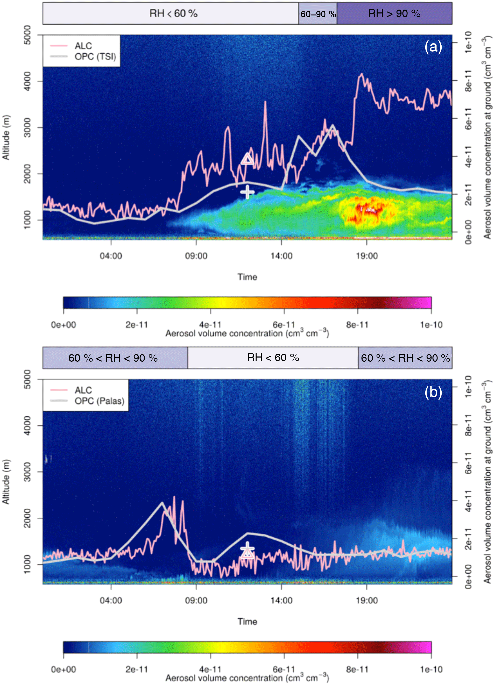
Figure 8Time–height cross section of the aerosol volume concentration at Saint-Christophe in the Aosta Valley for 29 December 2016 (a) and 5 September 2017 (b). The right y axis reports the volume concentration measured at the surface through TSI and Fidas® 200s OPCs (a, b, grey curves) and the ALC-derived volume concentration at 75 m (pink curves). The grey crosses and the pink triangles refer to the daily mean aerosol volume value derived by OPC and ALC measurements, respectively. The horizontal bars in the upper part of the panels indicate the ranges (RH<60 %, , and RH>90 %) of the measured in situ RH during the analyzed days.
The OPC-to-ALC comparison is certainly affected by intrinsic factors, such as differences in the atmospheric layer sampled (at ground and integrated between 0 and 75 m, for OPC and ALC, respectively) and in the probing methods (in situ and remote sensing, dried air sampled by OPC and ambient conditions sampled by the ALC). Furthermore, as mentioned in Sect. 4.2.1, a major critical issue of ALC retrievals at low levels is the correction for the overlap function, which needs to be experimentally characterized and verified for each instrument.
These issues are visible in the given examples of Fig. 8. In fact, in Fig. 8a, the agreement between the ALC-derived and the TSI OPC aerosol Va values is good between 00:00 and 07:00 UTC. In the following hours both instruments register an increase in the aerosol volume, although with some discrepancies in absolute values. Starting from 18:00 UTC, the ALC derives an aerosol volume concentration higher than the OPC concentration by a factor of 3–3.5. This disagreement could be related to both the presence/arrival of fine particles (<0.3 m) not measured by the optical counter (see for example Diémoz et al., 2018a), or to aerosol hygroscopic effects (increase in volume associated with hygroscopic growth seen by the ALC but not by the OPC that dries the air samples). This latter effect is confirmed by the large RH values (RH > 90 %) measured after 18:00 UTC. Figure 8b shows a good agreement between the ALC-derived and Fidas OPC Va values, in particular until 04:00 UTC and after 16:00 UTC. Some differences emerge around 07:00 UTC and between 11:00 and 15:00 UTC, when the ALC volume is lower by a factor of 2 compared to the in situ Fidas Va values. The smaller minimum detectable size of the Fidas OPC instrument with respect to the OPS is likely the reason for the better agreement between ALC and OPC Va values on this test date. In this case, the effect of RH seems to be less important, and indeed RH values remain lower than 90 %.
In general, high RH values (RH ≥90 %) are known to markedly affect the aerosol mass estimation from remote-sensing techniques and its relationship with reference PM2.5 or PM10 measurement methods, usually performed in dried conditions (e. g. Barnaba et al., 2010; Adam et al., 2012; Li et al., 2016, 2017). This theme is also discussed in Diémoz et al. (2018a) for the ALC measurement site of Fig. 8. Nevertheless, even with the mentioned limitations, results in Fig. 8 show the potential of the developed method in providing sound values of aerosol volume, and hence mass, in average-RH regimes well, giving support to more standard PM10 air quality monitoring.
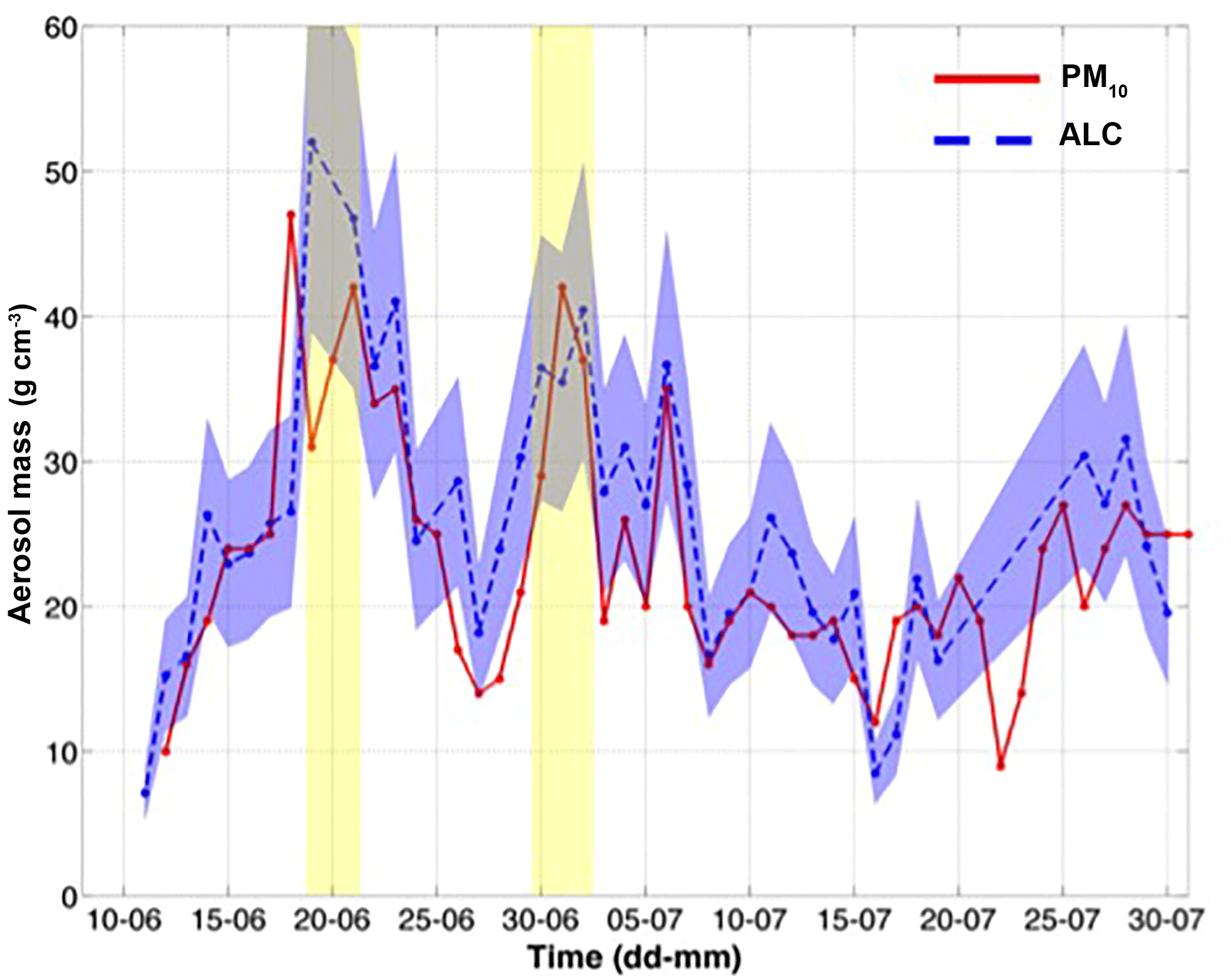
Figure 9Daily-resolved aerosol mass concentration at SPC, for the period June–July 2012, estimated from ALC-derived aerosol volume data at 225 m a.s.l. converted into mass using a fixed particle density ρa=2 g cm−3 (blue dotted line) and a variable ρa between 1.5 and 2.5 g cm−3 (shaded blue area). The red solid line is the daily PM10 concentration as measured by the local air quality agency (ARPA). Vertical yellow shaded stripes indicate the presence of dust events.
To give a further example in this direction, the model-assisted retrievals of aerosol mass over a longer time period were used to derive daily-mean aerosol mass concentrations (PM10, a measurement typical of air quality stations). For this purpose, for the 2-month period June–July 2012, we derived daily mean values of aerosol volume at the SPC site using the functional relationships Va=Va(βa) and then converted these into mass (PM10) using typical values of aerosol densities (ρa). Results are shown in Fig. 9. It compares the daily average PM10 concentration measured in situ at SPC by the Italian Regional Environmental Protection Agency (ARPA, red solid curve) and the model-assisted, ALC-derived daily mass concentration obtained assuming both a fixed particle density ρa=2 g cm−3 (blue dotted curve) and a range of particle density (1.5–2.5 g cm−3, shaded area), this range covering approximately the typical ρa values at the SPC site. Yellow shaded areas indicate the presence of dust events (e.g., Bucci et al., 2018) that are excluded from the results reported in the next paragraph.
More in detail, the daily-mean, ALC-derived mass concentrations were estimated in two steps: (1) estimation of hourly mass values for the selected height and (2) computation of the daily values through the median of the hourly values. To guarantee a good daily representativeness, the second step is applied only to those days on which at least 50 % of the hourly values are available in all the following temporal ranges: 00:00–05:00, 06:00–11:00, 12:00–17:00, and 18:00–23:00 UTC. Note that, due to the uncertainties associated with the O(z) in the first hundreds of meters (as previously mentioned, the ALC system at SPC has an old firmware, and its overlap function is not optimally characterized), we used the 225 m level as more trustworthy to estimate ALC mass concentration. Conversely, during the considered period of the year (i.e., June and July), the comparison to ground-level PM10 at SPC is expected to be only slightly affected by this height difference, particularly in daytime, due to the strong convection within the mixing layer. A possible exception could be in nocturnal conditions when vertical gradients in the lowermost hundreds of meters can occur. However, our statistical (3 year) ALC records show the mixing layer height at SPC to descend below 250 m only 4–5 h per day in July (usually between 22:00 and 03:00 UTC, i.e., when emissions are at a minimum). Overall, Fig. 9 confirms a good agreement between the ALC-derived and the ARPA reference PM10 values, with a correlation coefficient (R) of 0.64. In fact, mean, absolute mean, and relative differences between the two series are g cm−3, g cm−3, and . This agreement attests that the SPC site can indeed be considered an average continental site and suggests the potential of this approach to derive information on aerosol volume and mass. Still, due to the specificity of each site and to the limited period considered here, these results cannot be taken as representative of all continental sites at all times. Further studies at different places and over longer time periods would be necessary to better assess the uncertainty of the proposed retrieval, including uncertainties due to the variability in continental conditions (in terms of particle size distribution, compositions, hygroscopic effects, etc.) but also in the instrument-dependent performances (e.g., overlap corrections).
Thanks to their low construction and operation costs and to their capability of providing continuous, unattended measurements, the use of automated lidar ceilometers (ALCs) for aerosol characterization has increased in recent years. Several numerical approaches were recently proposed to estimate the aerosol vertical profile either using ceilometer measurements only or coupling these with ancillary measurements (e.g., Flentje et al., 2010; Wiegner and Geiß, 2012, 2014; Cazorla et al., 2017; Román et al., 2018).
This work proposes a methodology to retrieve key aerosol properties (such as extinction coefficient, surface area and volume, and thus mass) from lidar and ALC measurements using the results from a specifically developed aerosol numerical model to drive the retrievals. In particular, the numerical model uses a Monte Carlo approach to simulate a large set (20 000) of aerosol microphysical properties intended to reproduce the variability in average (clean to moderately polluted) continental conditions, i.e., those expected to dominate over Europe. Based on the assumption of particle sphericity, relevant computations of aerosol physical (surface area and volume, Sa and Va) and optical (backscattering and extinction coefficients, βa and αa, through Mie scattering theory) properties were performed at three commonly used lidar wavelengths (i.e., at the Nd:YAG laser harmonics 355, 532, and 1064 nm). Fitting procedures of this large set (20 000) of βa vs. αa, Sa, and Va data pairs were then used to derive mean functional relationships linking βa to αa, Sa, and Va, respectively. The model's statistical uncertainties (i.e., those related to the variability in the microphysical parameters used as input to the computations of the bulk physical–optical properties) associated with these so-derived mean relationships were found to be within 30 % and 40 % for βa vs. αa and βa vs. Va, respectively, while βa vs. Sa exhibits a larger dispersion (relative standard uncertainty of 40 %–70 %, depending on βa). It is worth mentioning that these are higher than those associated with the retrievals of aerosol bulk parameters using the complete set of Raman lidar observations (three aerosol backscattering and two extinction coefficients, i.e., the so-called 3+2 approach), assuming, as in our case, no random uncertainty in the lidar input data. For example, Veselovskii et al. (2012) found a maximum uncertainty of 15 % for particle volume and surface area estimation, in the case of 0 % random uncertainty in the lidar input data. Note, however, that such multiwavelength lidar systems are 10 to 20 times more expensive than ALC systems, need to be operated by highly trained operators, and are rarely run all day.
The model results also allowed exploration of the expected dependence of the (continental aerosol) lidar ratio (LR) on βa at 355, 532, and 1064 nm and, in turn, of the dependence of mean weighted-LR value at each wavelength (found to be 50.1±17.9, 49.6±16.0, and 37.7±12.6 sr, at 355, 532, and 1064 nm, respectively). LR values at 1064 nm in literature are scarce and their monotonic increase with βa found in this work (Fig. 3) suggests that the use of a fixed LR value for the inversion of ALC signals should be carried out with caution and carefully evaluated case by case. A similar, non-monotonic behavior characterizes the shapes of LR vs. the βa curve at 355 and 532 nm.
We tested the reliability of our model results in two ways: (1) the model numerical computations were compared to real lidar measurements (specifically selected within the EARLINET database), and (2) the model-assisted retrievals of aerosol optical (AOT) and physical (Va, PM10) properties by real operational ALC systems were compared to corresponding reference measurements performed by colocated independent instrumentation.
In particular, in task (1) our simulations were compared to backscatter and extinction coefficients at 532 and 355 nm independently retrieved by advanced Raman lidar systems operating at different EARLINET sites in Europe (namely Hamburg and Leipzig in Germany, Madrid in Spain, and Lecce and Potenza in Italy). The model simulations were found to statistically match the observations well (Figs. 4, 5, and C1). Mean discrepancies between model and measurement-based LR were found to be lower than 20 %, suggesting a good capability of the assumed aerosol model (and admitted range of variability) to represent real average continental aerosol conditions at different sites across Europe. Some differences emerged for southern Italian EARLINET sites, possibly affected by the influence of marine aerosols, leading to lower LR values for high values of βa.
For task (2) we applied the proposed model-based inversion to different ALC systems (Lufft CHM-15k), part of the Italian ALICEnet network. We first tested the ability of the proposed approach to derive aerosol extinction by comparing hourly-mean, vertically integrated αa (i.e., hourly mean AOT) derived by three ALC systems to corresponding AOT measurements from colocated sun photometers (ALICEnet sites of Aosta San Cristophe (ASC), San Pietro Capofiume (SPC), and Rome Tor Vergata (RTV), Fig. 7). ALC–sun photometer agreement was found to be within 30 %. Tests on the use of fixed LR were also performed to investigate the advantage of the proposed approach with respect to more standard ones. For this purpose, we used the (1064 nm) fixed-LR value suggested by the E-PROFILE EUMETSAT program and the weighted mean derived from our model (52 and 38 sr, respectively). While for the ASC site negligible differences were found among the three retrieval schemes, for both the SPC and RTV sites the best ALC–sun photometer agreement in AOT is reached when employing the model-based or the fixed-LR = 38 sr inversion schemes, with a mean error of around 16 %–19 % and 31 %–33 % for SPC and RTV, respectively. Applying the fixed LR value of 52 sr produces an overestimation of the AOT, with a mean relative bias equal to 33 % and 44 % at SPC and RTV, respectively. This suggests that, at 1064 nm, the LR value for continental aerosol is lower than the one assumed by the E-PROFILE procedure and, more in general, this highlights the advantage of a procedure not requiring an a priori, and to some extent arbitrary, choice of the LR value.
As a second test in task (2), values of aerosol volume (and mass) derived using the model-assisted ALC retrieval were compared to in situ aerosol measurements performed by OPCs and PM10 analyzers. A continuous, 2-month comparison (June–July 2012) between daily average aerosol mass concentration as measured in situ and derived by ALC (in the lowest altitudes) at SPC, showed a mean relative difference of around 15 % (Fig. 9).
Overall, the good results obtained in our validation efforts are encouraging but necessarily related to the specific conditions at the measuring sites considered and to the characteristics of the instruments employed. They are therefore not necessarily representative of results obtainable at all European continental sites, and at all times. Further tests using wider datasets covering a variety of sites and ALC instrumentation would be desirable to better understand potential and limits of the applicability of the proposed method over the larger scale. An obvious intrinsic limitation is that the method is dependent on the considered aerosol type, which in this study was tuned to reproduce average continental aerosol conditions. Errors associated with the application of the derived functional relationship might be larger if more specific aerosol conditions (e.g., contamination by sea salt or desert dust particles) affect a given site. In the future, the information coming from ALC systems with an additional depolarization channel (as tested in the DIAPASON project; Gobbi et al., 2018) could be used to force the retrieval to different model schemes (e.g., switching from “no dust” to “dust” scheme conditions) in the same vertical profile. This will enhance the capabilities of ALCs to operatively estimate and characterize the aerosol optical properties (e.g., Gasteiger and Freudenthaler, 2014).
Additionally, although our validation exercises returned results well within the uncertainties related to the model statistical variability alone (i.e., the relative errors associated with the mean functional relationships), the expected total uncertainty to be associated to the method should include terms that have not been specifically addressed in this work, as for example the instrumental error itself.
Conversely, the proposed approach has the main advantage of allowing the operational (i.e., 24/7) retrieval of fairly reliable remote-sensing profiles of aerosol optical (βa, αa) and physical (Sa, Va) properties (with associated uncertainties and limitations) by means of relatively simple and robust instruments. This could temporally and spatially complement the information coming from more advanced lidar networks (for example, the Raman channel of a multiwavelength system cannot be used in daylight conditions) and, more in general, could represent a valid option to deliver, in quasi-real time, the 3-D aerosol fields useful for operational air quality (e.g., integration of the in situ surface measurements) and for meteorological and climate monitoring (e.g., aerosol–cloud interaction and aerosol transport and dispersion processes).
AERONET Rome Tor Vergata sun photometer AOT data were downloaded from the AERONET web page (AERONET, 2018). SKYNET sun photometer AOT data were downloaded from the SKYNET web page (SKYNET, 2018). EARLINET backscattering and extinction coefficients were downloaded from the EARLINET web page (EARLINET, 2018). ALICEnet ALC raw data are available upon request at alicenet@isac.cnr.it.
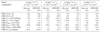
To evaluate the proposed continental model configuration (hereafter CM0) and discuss its sensitivity to the variability in the employed parameters, an overview of the impact on the model results produced by changing the limit of the variability ranges of these parameters (i.e., using different model configuration, CMX) is given in this section.
The varied model (CMX-CM0) mean difference on the considered optical property (OP) has been quantified through the following equation:
where Nbin is the total number of defined bins of βa.
The results of the mean differences of αa and LR for different ranges of βa and for the whole βa interval are reported in Table A1, in which relevant sensitivity cases (i.e., relative mean difference greater than 1 %) at λ=355 nm have been taken into account.
CM1 refers to a model configuration without the first aerosol mode (N1% =0). The overall decrease in the values of αa and LR (around 3 %–4 %) is due to the sum of significant and opposite effects for low and high values of βa for which 〈dαa∕αa〉 and 〈dLR∕LR〉 are of the order of −6 % and 8 %, respectively. Removing the coarser aerosol mode (N3% =0) causes positive mean values for 〈dαa∕αa〉 and 〈dLR∕LR〉 of the order of 5 % (sensitivity case CM2). In this case, the largest impact is observed for the βa range between and km−1 sr−1.
An opposite result is obtained by decreasing the upper bound of the r2 variability range (r2=0.03–0.05 µm, CM3). In fact this model configuration also leads to lower αa and LR values (〈dαa∕αa〉 and 〈dLR∕LR〉 are equal to −6 %, approximately). In this case, the variation in the r2 parameter affects the higher ranges of βa (– km−1 sr−1). Higher modal radii for the coarse-mode particle (r3=1–1.2 µm) in the CM4 configuration leads to the increase in the contribution of model-generated points with higher βa and causes lower values of αa and LR (〈dαa∕αa〉 and 〈dLR∕LR〉 are equal to −5 %, approximately) only for high values of βa (– km−1 sr−1), whereas the effect over the whole βa range is around −1 %.
The CM5 configuration accounts for the presence of more absorbing particles in the first aerosol mode, in which the lower bound of m1im has been increased by a factor of 10 (). This produces a significant effect only for the lower values of βa (– km−1 sr−1), with an increase in αa and LR of approximately 4 %. Conversely, increasing the lower bound of the real part of the second aerosol mode refractive index () has a large impact on the considered parameters. In fact, the CM6 configuration largely underestimates both αa and LR (around −15 % for both parameters) for all βa ranges.
The CM7 configuration refers to the impact of the total number of particles at the ground (Ntot). In this case, decreasing the upper bound of the variability range of Ntot by a factor of 2 (Ntot=500–5000 cm−3) lowers the mean values of αa and LR of around 5 %. Nevertheless, this effect is totally due to the contribution of the βa values between and km−1 sr−1, where and are around −10 %. Assuming no increase with altitude for σ1,2 (sensitivity case CM8) produces relevant differences in the mean values of αa and LR. In CM8, the overall overestimation of these two parameters is quite limited ( and ), whereas a large and opposite impact is observed for low and high values of βa. In fact, 〈dαa∕αa〉 (〈dLR∕LR〉) is equal to −14.1 (−13.9) and 18.5 (19.0) for – and – km−1 sr−1, respectively. As explained by Barnaba et al. (2007), the dependence of σ1,2 on the altitude can be associated with the fact that, when increasing the distance from the main aerosol sources, the particle processing is more efficient.
Table A1Mean differences of αa and LR among different model sensitivity cases and the proposed continental model configuration.
The parameters of the seventh-order polynomial fit used to derive the functional relationships between log(x) and log(y) (where x=βa and y=αa, Sa or Va) at λ=355 and 532 nm are reported in Tables B1 and B2, respectively.
Table B1Parameters of the seventh-order polynomial fits () for λ=355 nm, with x=log(βa) (in km−1 sr−1 unit) and , or Va) in km−1, cm2 cm−3, and cm3 cm−3, respectively.
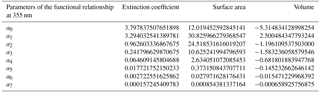
Table B2Parameters of the seventh-order polynomial fits () for λ=532 nm, with x=log(βa) (in km−1 sr−1 unit) and , or Va) in km−1, cm2 cm−3, and cm3 cm−3, respectively.

Figure C1 depicts the result of the comparison between EARLINET stations and our developed model (red and blue curves, respectively) in terms of mean LR per bin of βa at λ=532 nm. Note that only βa bins containing at least 1 % of the total modeled data were considered. Similar to the results at 355 nm shown in Sect. 4.1, a general good agreement between the modeled and the measured LR values is found. As attested by the low value of the mean discrepancy of Table 6, the modeled curve fits with Madrid observations well. Some major deviations are found for Lecce, which, however, at 532 nm, has a very low number of considered points (i.e., 109).
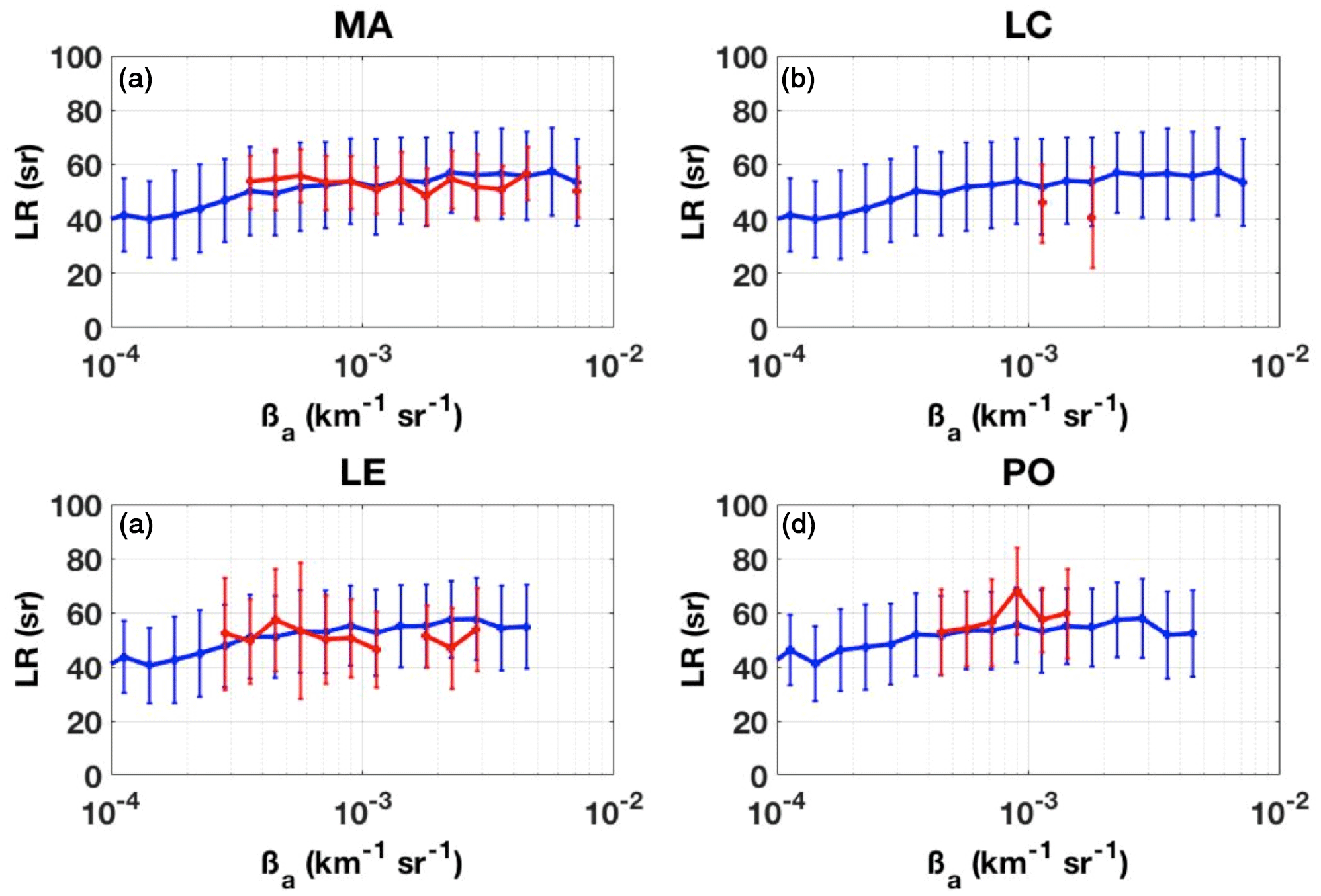
Figure C1Model-simulated (blue) and lidar-measured (red) LR vs. βa mean curves at 532 nm calculated per 10 equally spaced bins per decade of βa at the (a) Madrid (MA), (b) Lecce (LC), (c) Leipzig (LE), and (d) Potenza (PO) EARLINET lidar stations. Vertical bars are the associated standard deviations.
According to the results reported in Table A1, two model configurations (CM0a and CM0b) have been set up to better reproduce the EARLINET observations of LR vs. βa at the Lecce and Potenza sites. The comparison among these two configurations, the EARLINET measurements, and the CM0 setup is illustrated in Fig. D1 (panels a and b for Lecce and Potenza, respectively) in terms of LR mean value curves per 10 equally spaced bins per decade of βa. Blue and red colors have the same meaning as in Fig. 5 (i.e., CM0 model and observation curves, respectively); black curves refer to the LR vs. βa estimated through the CM0a and CM0b model versions for Lecce and Potenza stations, respectively. Vertical bars are the associated standard deviations.
The only difference between the CM0a and CM0 configurations consists in the upper bound of the variability range of Ntot (5000 vs. 10 000 cm−3 at ground, respectively). This modification seems to fit the observed LR vs. βa behavior at 355 nm. The upper bound Ntot value is similar to the one (i.e., Ntot upper bound = 3000 cm−3 at ground) used in the work of Barnaba et al. (2007) to characterize the optical properties of the continental aerosol present over southeastern Italy. The computed mean model–measurement LR relative difference between CM0a configuration and Lecce EARLINET measurements is around 5 %.
Similarly, the CM0b configuration uses the same value for the upper bound of Ntot variability range and, in addition, higher values of the r3 variability range of 1.0–1.2 vs. 0.3–0.5 µm, respectively. As highlighted by the panel b of Fig. D1, this model configuration allows a good reproduction of the LR vs. βa behavior derived by EARLINET lidar Raman measurements at 355 nm. This result seems to indicate the presence of coarser aerosols in a clean continental environment. In comparison to the CM0 model, the mean model–measurement LR relative difference decreases from 17 % to 6 %.
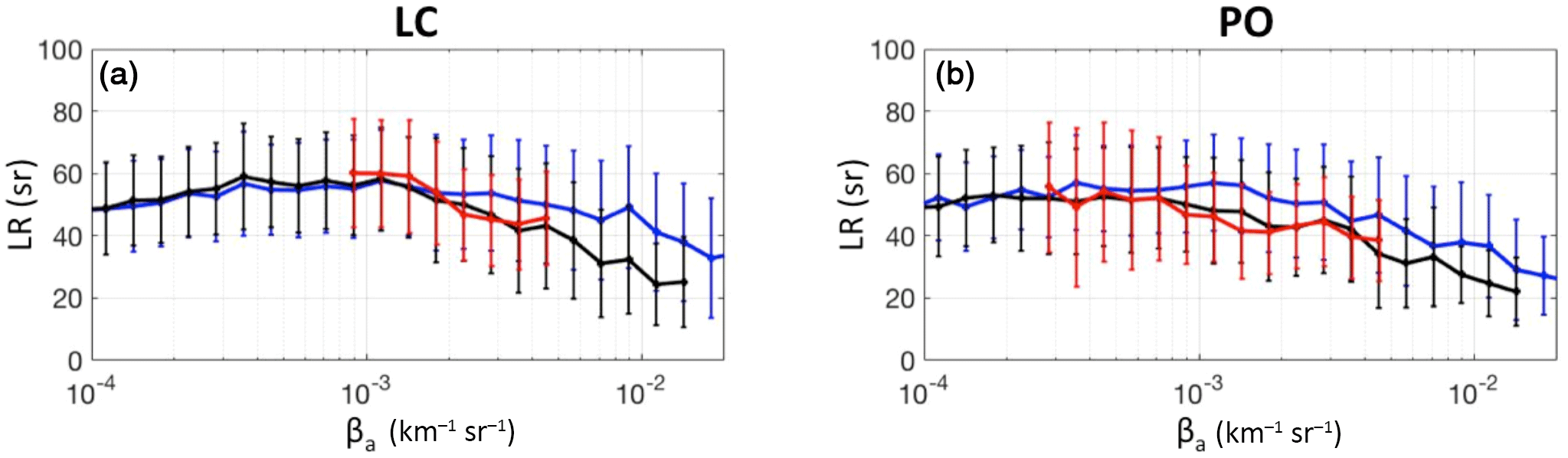
Figure D1Model-simulated (blue and black lines) and lidar-measured (red lines) LR vs. βa mean curves at 355 nm calculated per 10 equally spaced bins per decade of βa for the Lecce and Potenza EARLINET lidar stations (a, b, respectively). Blue refers to the CM0 model configuration and black to the CM0a and CM0b model configurations adapted to the Lecce and Potenza sites, respectively.
To gain a sense of both absolute and relative errors of AOT, in this section we report the scatter plots between the hourly-mean coincident AOTs at 1064 nm as derived with the ALC model-based approach and those measured at 1020 nm by the sun photometers installed at RTV, SPC, and ASC (Figs. E1, E2, and E3). The corresponding linear fit y=bx (red line), where x= sun photometer AOT and y= Nimbus CHM 15k AOT, is also shown in the plots. The values of the correlation coefficients for the three sites (R=0.77, R=0.72, and R=0.73 for RTV, SPC, and ASC, respectively) attest to a relatively good agreement between the two AOT measurements.
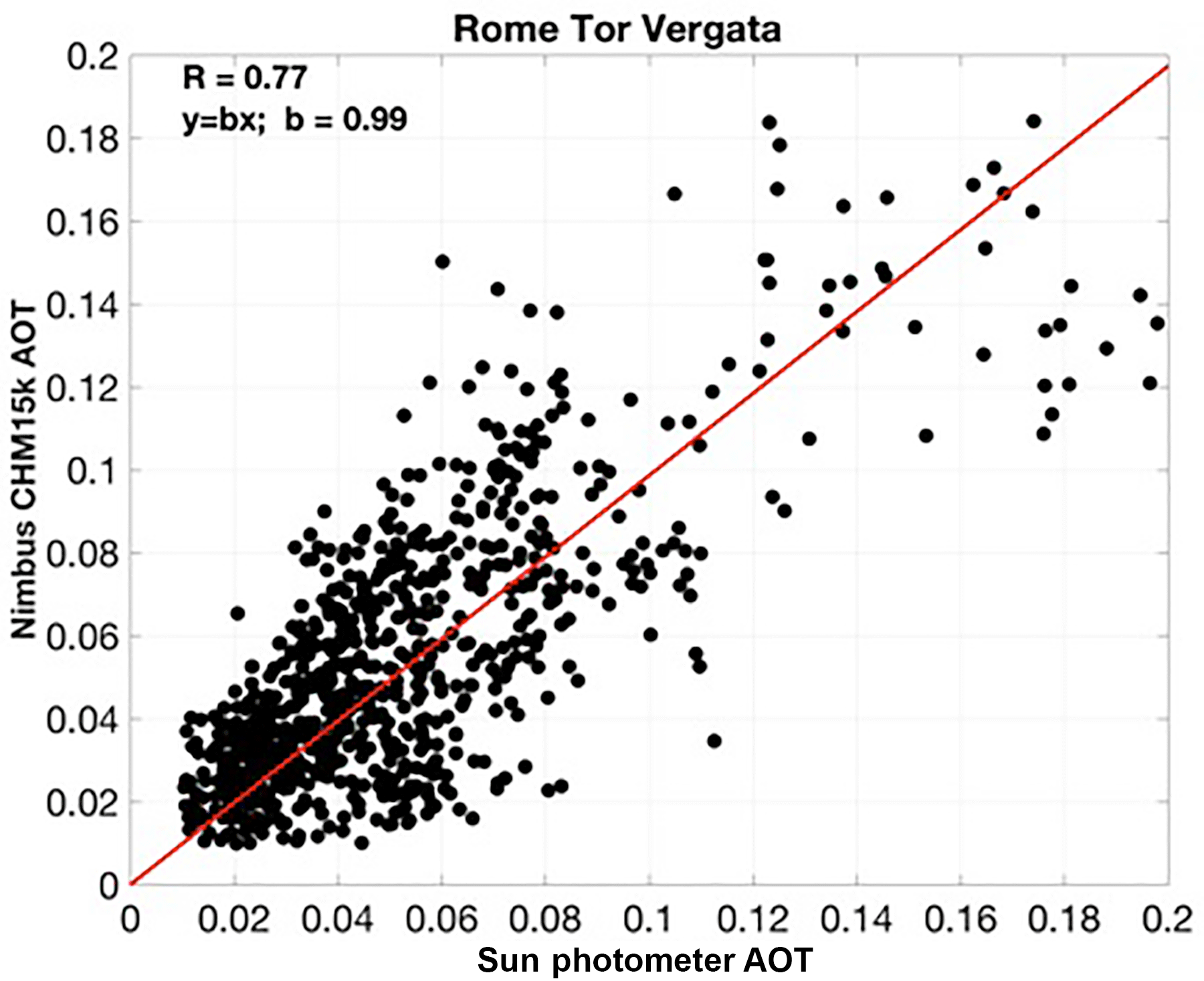
Figure E1Scatter plot between the hourly-mean coincident AOTs at 1064 nm as derived with the ALC model-based approach and measured at 1020 nm by the AERONET photometer at RTV. The red line represents the linear fit y=bx between the two datasets, where x is sun photometer AOT and y is Nimbus CHM 15k AOT.
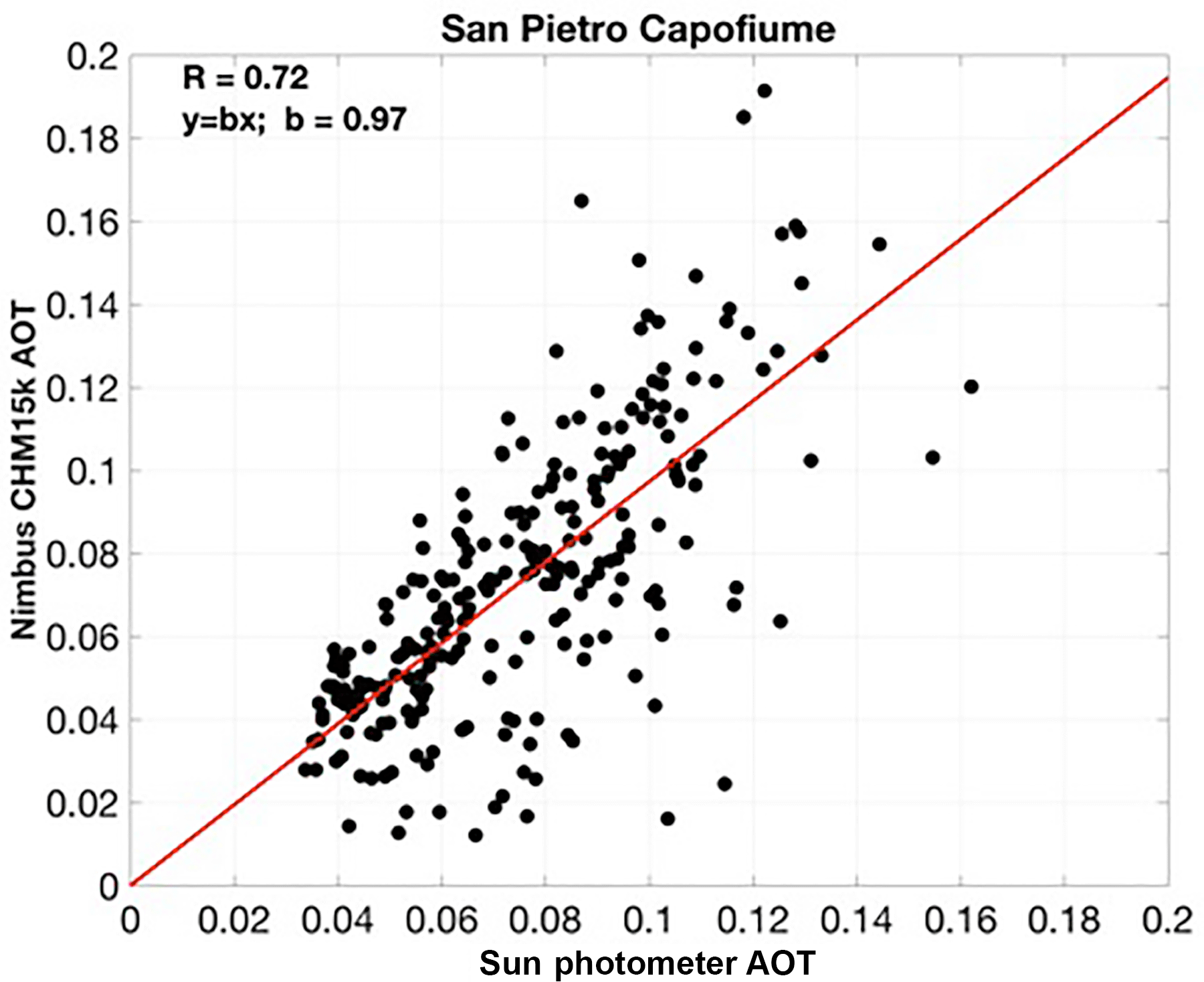
Figure E2Scatter plot between the hourly-mean coincident AOTs at 1064 nm as derived by the ALC model-based approach and measured at 1020 nm by the Skyrad photometer at SPC. The red line represents the linear fit y=bx between the two datasets, where x is sun photometer AOT and y is Nimbus CHM 15k AOT.
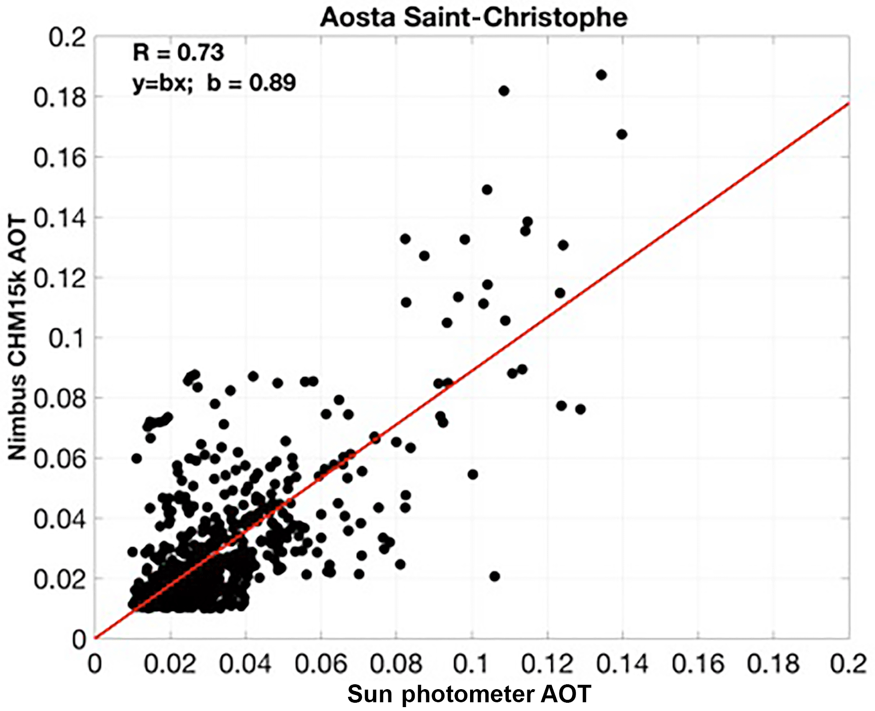
Figure E3Scatter plot between the hourly-mean coincident AOTs at 1064 nm as derived by the ALC model-based approach and measured at 1020 nm by the SKYRAD photometer at ASC. The red line represents the linear fit y=bx between the two datasets, where x is sun photometer AOT and y is Nimbus CHM 15k AOT.
DD, FB, and GPG conceived and designed the study. DD adapted the numerical model and performed the simulations. HD and LDL performed the ALC measurements in ASC and SPC, respectively. DD and HD implemented ALC inversion codes. DD performed most of the data analysis with contributions and advice from all co-authors. DD, FB, and GPG wrote the paper with input from all other co-authors.
The authors declare that they have no conflict of interest.
This article is part of the special issue “SKYNET – the international network for aerosol, clouds, and solar radiation studies and their applications (AMT/ACP inter-journal SI)”. It is not associated with a conference.
This work was partly supported by the European Commission LIFE+ project
“DIAPASON” (LIFE+2010 ENV/IT/391). The study also contributes to the
activities of the EU COST Action TOPROF (ES1303). The authors acknowledge
EARLINET for providing aerosol lidar profiles through its website (http://access.earlinet.org/, last access: 29 October 2018) and the EARLINET publishing group 2000–2010
(https://doi.org/10.1594/WDCC/EN_all_measurements_2000-2010). We thank the
EARLINET PIs Ulla Wandinger (Leibniz Institute for Tropospheric Research,
Leipzig, Germany), Manuel Pujadas (Centro de Investigaciones Energéticas,
Medioambientales y Tecnológicas, Department of Environment, Madrid,
Spain), Maria Rita Perrone (Department of Mathematics and Physics,
Universita' del Salento, Italy), and Aldo Amodeo (Istituto di Metodologie per
l'Analisi Ambientale, CNR-IMAA, Italy) and their staff for establishing,
maintaining, and running the EARLINET instruments at Leipzig (LE), Madrid
(MA), Lecce (LE), and Potenza (PO), respectively. ALC measurements at San
Pietro Capofiume (SPC) were partly funded by the Supersito project of the
Italian Emilia-Romagna region (DRG no. 428/10). The authors also thank Angelo
Lupi, Mauro Mazzola, and Vito Vitale (ISAC-CNR) for the management of the
PREDE POM-02L sun–sky radiometer measurements at SPC. AOT data analysis for
San Pietro Capofiume and Saint-Christophe in the Aosta Valley was performed as part of a
cooperative activity with the SKYNET network. We also acknowledge the AERONET
team for the processing of the Rome Tor Vergata data used in this research
effort.
Edited by: M.
Campanelli
Reviewed by: three anonymous referees
Adam, M., Putaud, J. P., Martins dos Santos, S., Dell'Acqua, A., and Gruening, C.: Aerosol hygroscopicity at a regional background site (Ispra) in Northern Italy, Atmos. Chem. Phys., 12, 5703–5717, https://doi.org/10.5194/acp-12-5703-2012, 2012.
AERONET: AERONET aerosol data base, available at: http://aeronet.gsfc.nasa.gov/, last access: April 2018.
Amiridis, V., Marinou, E., Tsekeri, A., Wandinger, U., Schwarz, A., Giannakaki, E., Mamouri, R., Kokkalis, P., Binietoglou, I., Solomos, S., Herekakis, T., Kazadzis, S., Gerasopoulos, E., Proestakis, E., Kottas, M., Balis, D., Papayannis, A., Kontoes, C., Kourtidis, K., Papagiannopoulos, N., Mona, L., Pappalardo, G., Le Rille, O., and Ansmann, A.: LIVAS: a 3-D multi-wavelength aerosol/cloud database based on CALIPSO and EARLINET, Atmos. Chem. Phys., 15, 7127–7153, https://doi.org/10.5194/acp-15-7127-2015, 2015.
Ansmann, A., Wandinger, U., Riebesell, M., Weitkamp, C., and Michaelis, W.: Independent measurement of extinction and backscatter profiles in cirrus clouds by using a combined Raman elastic-backscatter lidar, Appl. Optics, 31, 7113–7131, 1992.
Ansmann, A., Tesche, M., Seifert, P., Groß, S., Freudenthaler, V., Apituley, A., Wilson, K. M., Serikov, I., Linné, H., Heinold, B., Hiebsch, A., Schnell, F., Schmidt, J., Mattis, I., Wandinger, U., and Wiegner, M.: Ash and fine-mode particle mass profiles from EARLINET-AERONET observations over central Europe after the eruptions of the Eyjafjallajökull volcano in 2010, J. Geophys. Res., 116, D00U02, https://doi.org/10.1029/2010JD015567, 2011a.
Ansmann, A., Petzold, A., Kandler, K., Tegen, I., Wendisch, M., Müller, D., Weinzierl, B., Müller, T., and Heintzenberg, J.: Saharan mineral dust experiments SAMUM-1 and SAMUM-2: What have we learned?, Tellus B, 63, 403–429, https://doi.org/10.1111/j.1600-0889.2011.00555.x, 2011b.
Ansmann, A., Seifert, P., Tesche, M., and Wandinger, U.: Profiling of fine and coarse particle mass: case studies of Saharan dust and Eyjafjallajökull/Grimsvötn volcanic plumes, Atmos. Chem. Phys., 12, 9399–9415, https://doi.org/10.5194/acp-12-9399-2012, 2012.
Barnaba, F. and Gobbi, G. P.: Lidar estimation of tropospheric aerosol extinction, surface area and volume: Maritime and desert-dust cases, J. Geophys. Res., 106, 3005–3018, 2001.
Barnaba, F. and Gobbi, G. P.: Modeling the aerosol extinction versus backscatter relationship for lidar applications: maritime and continental conditions, J. Atmos. Ocean. Technol., 21, 428–442, 2004a.
Barnaba, F. and Gobbi, G. P.: Aerosol seasonal variability over the Mediterranean region and relative impact of maritime, continental and Saharan dust particles over the basin from MODIS data in the year 2001, Atmos. Chem. Phys., 4, 2367–2391, https://doi.org/10.5194/acp-4-2367-2004, 2004b.
Barnaba, F., De Tomasi, F., Gobbi, G. P., Perrone, M. R., Tafuro A., Extinction versus backscatter relationships for lidar applications at 351 nm: maritime and desert aerosol simulations and comparison with observations, Atmos. Res., 70, 229–259, https://doi.org/10.1016/j.atmosres.2004.02.001, 2004.
Barnaba, F., Tafuro, A. M., De Tomasi, F., and Perrone, M. R.: Observed and simulated vertically resolved optical properties of continental aerosols over southeastern Italy: A closure study, J. Geophys. Res., 112, D10203, https://doi.org/10.1029/2006JD007926, 2007.
Barnaba, F., Putaud, J. P., Gruening, C., dell'Acqua, A., and Dos Santos, S.: Annual cycle in co-located in situ, total-column, and height-resolved aerosol observations in the Po Valley (Italy): Implications for ground-level particulate matter mass concentration estimation from remote sensing, J. Geophys. Res., 115, D19209, https://doi.org/10.1029/2009JD013002, 2010.
Barnaba, F., Bolignano, A., Di Liberto, L., Morelli, M., Lucarelli, F., Nava, S., Perrino, C., Canepari, S., Basart, S., Costabile, F., Dionisi, D., Ciampichetti, S., Sozzi, R., and Gobbi, G. P.: Desert dust contribution to PM10 loads in Italy: Methods and recommendations addressing the relevant European Commission Guidelines in support to the Air Quality Directive 2008/50/EC, Atmos. Environ., 161, 288–305, https://doi.org/10.1016/j.atmosenv.2017.04.038, 2017.
Bohren, C. F. and Huffman, D. R.: Absorption and Scattering of Light by Small Particles, Wiley-Interscience, New York, 103, 119–122, 477, 1983.
Bösenberg, J., Ansmann, A., Baldasano, J. M., Balis, D., Böckmann, C., Calpini, B., Chaikovsky, A., Flamant, P., Hagard, A., Mitev, V., Papayannis, A., Pelon, J., Resendes, D., Schneider, J., Spinelli, N., Trickl, T., Vaughan, G., Visconti, G., and Wiegner, M.: EARLINET: a European Aerosol Research Lidar Network, in: Advances in Laser Remote Sensing, edited by: Dabas, A., Loth, C., and Pelon, J., Ecole polytechnique, Palaiseau Cedex, France, 155–158, 2001.
Bösenberg, J., Matthias, V., Amodeo, A., Amoiridis, V., Ansmann, A., Baldasano, J. M., Balin, I., Balis, D., Böckmann, C., Boselli, A., Carlsson, G., Chaikovsky, A., Chourdakis, G., Comerón, A., De Tomasi, F., Eixmann, R., Freudenthaler, V., Giehl, H., Grigorov, I., Hågård, A., Iarlori, M., Kirsche, A., Kolarov, G., Komguem, L., Kreipl, S., Kumpf, W., Larchevêque, G., Linné, H., Matthey, R., Mattis, I., Mekler, A., Mironova, I., Mitev, V., Mona, L., Müller, D., Music, S., Nickovic, S., Pandolfi, M., Papayannis, A., Pappalardo, G., Pelon, J., Pérez, C., Perrone, R. M., Persson, R., Resendes, D. P., Rizi, V., Rocadenbosch, F., Rodrigues, A., Sauvage, L., Schneidenbach, L., Schumacher, R., Shcherbakov, V., Simeonov, V., Sobolewski, P., Spinelli, N., Stachlewska, I., Stoyanov, D., Trickl, T., Tsaknakis, G., Vaughan, G., Wandinger, U., Wang, X., Wiegner, M., Zavrtanik, M., and Zerefos. C.: EARLINET: A European Aerosol Research Lidar Network to Establish an Aerosol Climatology, Max-Planck-Institut Report No. 348, 2003.
Bucci, S., Cristofanelli, P., Decesari, S., Marinoni, A., Sandrini, S., Größ, J., Wiedensohler, A., Di Marco, C. F., Nemitz, E., Cairo, F., Di Liberto, L., and Fierli, F.: Vertical distribution of aerosol optical properties in the Po Valley during the 2012 summer campaigns, Atmos. Chem. Phys., 18, 5371–5389, https://doi.org/10.5194/acp-18-5371-2018, 2018.
Cazorla, A., Casquero-Vera, J. A., Román, R., Guerrero-Rascado, J. L., Toledano, C., Cachorro, V. E., Orza, J. A. G., Cancillo, M. L., Serrano, A., Titos, G., Pandolfi, M., Alastuey, A., Hanrieder, N., and Alados-Arboledas, L.: Near-real-time processing of a ceilometer network assisted with sun-photometer data: monitoring a dust outbreak over the Iberian Peninsula, Atmos. Chem. Phys., 17, 11861–11876, https://doi.org/10.5194/acp-17-11861-2017, 2017.
d'Almeida, G. A., Koepke, P., and Shettle, E. P.: Atmospheric Aerosol-Global Climatology and Radiative Characteristics, A. Deepack Hampton, VA, 561 pp., 1991.
D'Amato, G., Baena-Cagnani, C. E., Cecchi, L., Annesi-Maesano, I., Nunes, C., Ansotegui, I., D'Amato, M., Licciardi, G., Sofia, M., and Canonica, W. G.: Climate change, air pollution and extreme events leading to increasing prevalence of allergic respiratory diseases, Multidiscip. Resp. Med., 8, 8–12, https://doi.org/10.1186/2049-6958-8-12, 2013.
De Tomasi, F., Tafuro, A. M., and Perrone, M. R.: Height and seasonal dependence of aerosol optical properties over south-east Italy, J. Geophys. Res., 111, D10203, https://doi.org/10.1029/2005JD006779, 2006.
Diémoz, H., Campanelli, M., Estelles, V.: One Year of Measurements with a POM-02 Sky Radiometer at an Alpine EuroSkyRad Station, J. Meteorol. Soc. Jpn., 92A, 1–16, 2014.
Diémoz, H., Barnaba, F., Magri, T., Pession, G., Dionisi, D., Pittavino, S., Tombolato, I. K. F., Campanelli, M., Della Ceca, L. S., Hervo, M., Di Liberto, L., Ferrero, L., and Gobbi, G. P.: Transport of Po Valley aerosol pollution to the northwestern Alps. Part 1: phenomenology, Atmos. Chem. Phys. Discuss., https://doi.org/10.5194/acp-2018-960, in review, 2018a.
Diémoz, H., Barnaba, F., Magri, T., Pession, G., Pittavino, S., Tombolato, I. K. F., M., Campanelli, M. and Gobbi, G. P.: Transport of Po Valley aerosol pollution to the northwestern Alps. Part 2: long-term impact on air quality, Atmos. Chem. Phys., in preparation, 2018b.
Dinar, E., Abo Riziq, A., Spindler, C., Erlick, C., Kiss, G., and Rudich, Y.: The complex refractive index of atmospheric and model humic-like substances (HULIS) retrieved by a cavity ring down aerosol spectrometer (CRD-AS), Faraday Discuss., 137, 279–295, 2008.
Dionisi, D., Keckhut, P., Liberti, G. L., Cardillo, F., and Congeduti, F.: Midlatitude cirrus classification at Rome Tor Vergata through a multichannel Raman-Mie-Rayleigh lidar, Atmos. Chem. Phys., 13, 11853–11868, https://doi.org/10.5194/acp-13-11853-2013, 2013.
Düsing, S., Wehner, B., Seifert, P., Ansmann, A., Baars, H., Ditas, F., Henning, S., Ma, N., Poulain, L., Siebert, H., Wiedensohler, A., and Macke, A.: Helicopter-borne observations of the continental background aerosol in combination with remote sensing and ground-based measurements, Atmos. Chem. Phys., 18, 1263–1290, https://doi.org/10.5194/acp-18-1263-2018, 2018.
EARLINET: EARLINET data base, available at: http://www.earlinet.org, last access: 11 January 2018.
EC: Directive 2008/50/EC of the European Parliament and of the Council of 21 May 2008 on Ambient Air Quality and Cleaner Air for Europe, OJ L 152, 11.6.2008, 1e44, available at: https://eur-lex.europa.eu/LexUriServ/LexUriServ.do?uri=OJ:L:2008:152:0001:0044:EN:PDF (last access: 19 October 2018), 2008.
Feingold, G., McComiskey, A., Yamaguchi, T., Johnson, J. S., Carslaw, K. S., and Schmidt, K. S.: New approaches to quantifying aerosol influence on the cloud radiative effect, P. Natl. Acad. Sci. USA, 113, 5812–5819, 2016.
Fernald, F. G., Herman, B. M., and Reagan J. A.: Determination of Aerosol Height Distributions by Lidar, J. Appl. Meteor., 11, 482–489, https://doi.org/10.1175/1520-0450(1972)011<0482:DOAHDB>2.0.CO;2, 1972.
Flentje, H., Claude, H., Elste, T., Gilge, S., Köhler, U., Plass-Dülmer, C., Steinbrecht, W., Thomas, W., Werner, A., and Fricke, W.: The Eyjafjallajökull eruption in April 2010 – detection of volcanic plume using in-situ measurements, ozone sondes and lidar-ceilometer profiles, Atmos. Chem. Phys., 10, 10085–10092, https://doi.org/10.5194/acp-10-10085-2010, 2010.
Gasteiger, J., Groß, S., Freudenthaler, V., and Wiegner, M.: Volcanic ash from Iceland over Munich: mass concentration retrieved from ground-based remote sensing measurements, Atmos. Chem. Phys., 11, 2209–2223, https://doi.org/10.5194/acp-11-2209-2011, 2011.
Gasteiger, J. and Freudenthaler, V.: Benefit of depolarization ratio at λ=1064 nm for the retrieval of the aerosol microphysics from lidar measurements, Atmos. Meas. Tech., 7, 3773–3781, https://doi.org/10.5194/amt-7-3773-2014, 2014.
Gobbi, G. P.: Lidar estimation of stratospheric aerosol properties: Surface, volume, and extinction to backscatter ratio, J. Geophys. Res., 100, 11219–11235, 1995.
Gobbi, G. P., Barnaba, F. Di Liberto, L., Bolignano, A., Lucarelli, F., Nava, S., Perrino, C., Pietrodangelo, A., Basar, S., Costabile, F., Dionisi, D., Rizza, U., Canepari, S., Sozzi, R., Morelli, M., Manigrasso, M., Drewnick, R. F., Struckmeier, C., Poenitz, K., and Wille, H.: An integrated view of Saharan Dust Advections to Italy and the Central Mediterranean: Main Outcomes of the “DIAPASON” Project, Atmos. Environ., in review, 2018.
Hand, J. L. and Malm, W. C.: Review of aerosol mass scattering efficiencies from ground-based measurements since 1990, J. Geophys. Res., 112, D16203, https://doi.org/10.1029/2007JD008484, 2007.
Haywood, J. M. and Boucher, O.: Estimates of the direct and indirect radiative forcing due to tropospheric aerosols: A review, Rev. Geophys., 38, 513–543, 2000.
He, T.-Y., Stanic, S., Gao, F., Bergant, K., Veberic, D., Song, X.-Q., and Dolžan, A.: Tracking of urban aerosols using combined LIDAR-based remote sensing and ground-based measurements, Atmos. Meas. Tech., 5, 891–900, https://doi.org/10.5194/amt-5-891-2012, 2012.
Heese, B. and Wiegner, M.: Vertical aerosol profiles from Raman polarization lidar observations during the dry season AMMA field campaign, J. Geophys. Res.- Atmos., 113, D00C11, https://doi.org/10.1029/2007JD009487, 2008.
Heese, B., Flentje, H., Althausen, D., Ansmann, A., and Frey, S.: Ceilometer lidar comparison: backscatter coefficient retrieval and signal-to-noise ratio determination, Atmos. Meas. Tech., 3, 1763–1770, https://doi.org/10.5194/amt-3-1763-2010, 2010.
Hervo, M., Poltera, Y., and Haefele, A.: An empirical method to correct for temperature-dependent variations in the overlap function of CHM15k ceilometers, Atmos. Meas. Tech., 9, 2947–2959, https://doi.org/10.5194/amt-9-2947-2016, 2016.
Hess, M., Koepke, P., and Schult, I.: Optical properties of aerosols and clouds: The software package OPAC, B. Am. Meteor. Soc., 79, 831–844, 1998.
Holben, B. N., Eck, T. F., Slutsker, I., Tanré, D., Buis, J. P., Setzer, A., Vermote, E.; Reagan, J. A.; Kaufman, Y. J., Nakajima, T., Lavenu, F., Jankowiak, I., and Smirnov, A.: AERONET – A federated instrument network and data archive for aerosol characterization, Remote Sens. Environ., 66, 1–16, https://doi.org/10.1016/S0034-4257(98)00031-5, 1998.
Klett, J. D.: Stable analytical inversion solution for processing lidar returns, Appl. Optics, 20, 211–220, 1981.
Klett, J. D.: Lidar inversion with variable backscatter/extinction ratios, Appl. Opt., 24, 1638–1643, https://doi.org/10.1364/AO.24.001638, 1985.
Koetz, B., Sun, G., Morsdorf, F., Ranson, K.J., Kneubuhler, M., Itten, K., and Allgower, B.: Inversion of Combined Radiative Transfer Models for Imaging Spectrometer and LIDAR Data, 2006 IEEE International Symposium on Geoscience and Remote Sensing, Denver, CO, 31 July–4 August 2006, 395–398, https://doi.org/10.1109/IGARSS.2006.106, 2006.
Kovalev, V. A. and Eichinger, W. E.: Elastic Lidar, Theory, Practice, and Analysis Methods, 615 pp., John Wiley & Sons, Weinheim, Germany, 2004.
Lelieveld, J., Evans, J. S., Fnais, M., Giannadaki, D., and Pozzer, A.: The contribution of outdoor air pollution sources to premature mortality on a global scale, Nature, 525, 367–371, 2015.
Levy, R. C., Remer, L. A., and Dubovik, O.: Global aerosol optical properties and application to Moderate Resolution Imaging Spectroradiometer aerosol retrieval over land, J. Geophys. Res., 112, D13210, https://doi.org/10.1029/2006JD007815, 2007.
Lewandowski, P. A., Eichinger, W. E., Holder, H., Prueger, J., Wang, J., and Kleinman, L. I.: Vertical distribution of aerosols in the vicinity of Mexico City during MILAGRO-2006 Campaign, Atmos. Chem. Phys., 10, 1017–1030, https://doi.org/10.5194/acp-10-1017-2010, 2010.
Li, S., Joseph, E., and Min, Q.: Remote sensing of ground-level PM2.5 combining AOD and backscattering profile, Remote Sens. Environ., 183, 120–128, https://doi.org/10.1016/j.rse.2016.05.025, 2016.
Li, S., Joseph, E., Min, Q., Yin, B., Sakai, R., and Payne, M. K.: Remote sensing of PM2.5 during cloudy and nighttime periods using ceilometer backscatter, Atmos. Meas. Tech., 10, 2093–2104, https://doi.org/10.5194/amt-10-2093-2017, 2017.
Lohmann, U. and Feichter, J.: Global indirect aerosol effects: a review, Atmos. Chem. Phys., 5, 715–737, https://doi.org/10.5194/acp-5-715-2005, 2005.
Lolli, S., Madonna, F., Rosoldi, M., Campbell, J. R., Welton, E. J., Lewis, J. R., Gu, Y., and Pappalardo, G.: Impact of varying lidar measurement and data processing techniques in evaluating cirrus cloud and aerosol direct radiative effects, Atmos. Meas. Tech., 11, 1639–1651, https://doi.org/10.5194/amt-11-1639-2018, 2018.
Madonna, F., Amodeo, A., Boselli, A., Cornacchia, C., Cuomo, V., D'Amico, G., Giunta, A., Mona, L., and Pappalardo, G.: CIAO: the CNR-IMAA advanced observatory for atmospheric research, Atmos. Meas. Tech., 4, 1191–1208, https://doi.org/10.5194/amt-4-1191-2011, 2011.
Madonna, F., Amato, F., Vande Hey, J., and Pappalardo, G.: Ceilometer aerosol profiling versus Raman lidar in the frame of the INTERACT campaign of ACTRIS, Atmos. Meas. Tech., 8, 2207–2223, https://doi.org/10.5194/amt-8-2207-2015, 2015.
Madonna, F., Rosoldi, M., Lolli, S., Amato, F., Vande Hey, J., Dhillon, R., Zheng, Y., Brettle, M., and Pappalardo, G.: Intercomparison of aerosol measurements performed with multi-wavelength Raman lidars, automatic lidars and ceilometers in the framework of INTERACT-II campaign, Atmos. Meas. Tech., 11, 2459–2475, https://doi.org/10.5194/amt-11-2459-2018, 2018.
Mamali, D., Marinou, E., Sciare, J., Pikridas, M., Kokkalis, P., Kottas, M., Binietoglou, I., Tsekeri, A., Keleshis, C., Engelmann, R., Baars, H., Ansmann, A., Amiridis, V., Russchenberg, H., and Biskos, G.: Vertical profiles of aerosol mass concentration derived by unmanned airborne in situ and remote sensing instruments during dust events, Atmos. Meas. Tech., 11, 2897–2910, https://doi.org/10.5194/amt-11-2897-2018, 2018.
Mamouri, R.-E. and Ansmann, A.: Potential of polarization lidar to provide profiles of CCN- and INP-relevant aerosol parameters, Atmos. Chem. Phys., 16, 5905–5931, https://doi.org/10.5194/acp-16-5905-2016, 2016.
Matthias, V. and Bösenberg, J.: Aerosol climatology for the planetary boundary layer derived from regular lidar measurements, Atmos. Res., 63, 221–245, 2002.
McGill, M. J., Yorks, J. E., Scott, V. S., Kupchock, A. W., and Selmer, P. A.: The Cloud-Aerosol Transport System (CATS): A technology demonstration on the International Space Station, in: Lidar Remote Sensing for Environmental Monitoring XV (vol. 9612, p. 96120A), International Society for Optics and Photonics, Proc. SPIE, 9612, 96120A, https://doi.org/10.1117/12.2190841, 2015.
Menut, L., Flamant, C., Pelon, J., Valentin, R., Flamant, P. H., Dupont, E., and Carissimo, B.: Study of the boundary layer structure over the Paris agglomeration as observed during the ECLAP Experiment, in: Advances in atmospheric remote sensing with lidar, edited by: Ansmann, A., Neuber, R., Rairoux, P., and Wandinger, U., Springer, Berlin, 15–18, 1997.
Mishchenko, M. I., Travis, L. D., Kahn, R. A., and West, R. A.: Modeling phase functions for dustlike tropospheric aerosols using a mixture of randomly oriented polydisperse spheroids. J. Geophys. Res., 102, 16831–16847, https://doi.org/10.1029/96JD02110, 1997.
Mona, L., Amodeo, A., Pandolfi, M., and Pappalardo, G.: Saharan dust intrusions in the Mediterranean area: Three years of Raman lidar measurements, J. Geophys. Res., 111, D16203, https://doi.org/10.1029/2005JD006569, 2006.
Omar, A. H., Winker, D. M., Kittaka, C., Vaughan, M. A., Liu, Z. Y., Hu, Y. X., Trepte, C. R., Rogers, R. R., Ferrare, R. A., Lee, K. P., Kuehn, R. E., and Hostetler, C. A.: The CALIPSO automated aerosol classification and lidar ratio selection algorithm, J. Atmos. Ocean. Tech., 26, 1994–2014, https://doi.org/10.1175/2009jtecha1231.1, 2009.
Papagiannopoulos, N., Mona, L., Alados-Arboledas, L., Amiridis, V., Baars, H., Binietoglou, I., Bortoli, D., D'Amico, G., Giunta, A., Guerrero-Rascado, J. L., Schwarz, A., Pereira, S., Spinelli, N., Wandinger, U., Wang, X., and Pappalardo, G.: CALIPSO climatological products: evaluation and suggestions from EARLINET, Atmos. Chem. Phys., 16, 2341–2357, https://doi.org/10.5194/acp-16-2341-2016, 2016.
Pappalardo, G., Wandinger, U., Mona, L., Hiebsch, A., Mattis, I., Amodeo, A., Ansmann, A., Seifert, P., Linne, H., Apituley, A., Alados Arboledas, L., Balis, D., Chaikovsky, A., D'Amico, G., De Tomasi, F., Freudenthaler, V., Giannakaki, E., Giunta, A., Grigorov, I., Iarlori, M., Madonna, F., Mamouri, R.-E., Nasti, L., Papayannis, A., Pietruczuk, A., Pujadas, M., Rizi, V., Rocadenbosch, F., Russo, F., Schnell, F., Spinelli, N.,Wang, X., and Wiegner, M.: EARLINET correlative measurements for CALIPSO: first intercomparison results, J. Geophys. Res., 115, D00H19, https://doi.org/10.1029/2009JD012147, 2010.
Pappalardo, G., Amodeo, A., Apituley, A., Comeron, A., Freudenthaler, V., Linné, H., Ansmann, A., Bösenberg, J., D'Amico, G., Mattis, I., Mona, L., Wandinger, U., Amiridis, V., Alados-Arboledas, L., Nicolae, D., and Wiegner, M.: EARLINET: towards an advanced sustainable European aerosol lidar network, Atmos. Meas. Tech., 7, 2389–2409, https://doi.org/10.5194/amt-7-2389-2014, 2014.
Patterson, E. M., Kiang, C. S., Delany, A. C., Wartburg, A. F., Leslie, D., and Huebert, B. J: Global measurements of aerosols in remote continental and marine regions: Concentrations, size distributions, and optical properties, J. Geophys. Res., 85, 7361–7375, 1980.
Perrone, M. R., De Tomasi, F., and Gobbi, G. P.: Vertically resolved aerosol properties by multi-wavelength lidar measurements, Atmos. Chem. Phys., 14, 1185–1204, https://doi.org/10.5194/acp-14-1185-2014, 2014.
Pletscher, K., Weiss, M., and Moelter, L.: Simultaneous determination of PM fractions, particle number and particle size distribution in high time resolution applying one and the same optical measurement technique, Gefahrst. Reinhalt. L., 76, 425–436, 2016.
Putaud, J.-P., Van Dingenen, R., Alastuey, A., Bauer, H., Birmili, W., Cyrys, J., Flentje, H., Fuzzi, S., Gehrig, R., Hansson, H. C., Harrison, R. M., Herrmann, H., Hitzenberger, R., Huglin, C.,Jones, A. M., Kasper-Giebl, A., Kiss, G., Kousa, A., Kuhlbusch, T. A. J., Loschau, G., Maenhaut, W., Molnar, A., Moreno, T., Pekkanen, J., Perrino, C., Pitz, M., Puxbaum, H., Querol, X., Rodriguez, S., Salma, I., Schwarz, J., Smolik, J., Schneider, J., Spindler, G., ten Brink, H., Tursic, J., Viana, M., Wiedensohler, A., and Raes, F.: A European aerosol phenomenology – 3: physical and chemical characteristics of particulate matter from 60 rural, urban, and kerbside sites across Europe, Atmos. Environ., 44, 1308–1320, 2010.
Román, R., Benavent-Oltra, J. A., Casquero-Vera, J. A., Lopatin, A., Cazorla, A., Lyamani, H., Denjean, C., Fuertes, D. Pérez-Ramírez, D., Torres, B., Toledano, C., Dubovik, O., Cachorro, V. E., de Frutos, A. M., Olmo, F. J., and Alados-Arboledas, L.: Retrieval of aerosol profiles combining sunphotometer and ceilometer measurements in GRASP code, Atmos. Res., 204, 161–177, https://doi.org/10.1016/j.atmosres.2018.01.021, 2018.
Shipley, S. T., Tracy, D. H., Eloranta, E. W., Tauger, J. T., Sroga, J. T., Roesler, F. L., and Weinman J. A.: High spectral resolution lidar to measure optical scattering properties of atmospheric aerosols, 1: Theory and instrumentation, Appl. Opt. 22, 3716–3724, 1983.
Sicard, M., Guerrero-Rascado, J. L., Navas-Guzmán, F., Preißler, J., Molero, F., Tomás, S., Bravo-Aranda, J. A., Comerón, A., Rocadenbosch, F., Wagner, F., Pujadas, M., and Alados-Arboledas, L.: Monitoring of the Eyjafjallajökull volcanic aerosol plume over the Iberian Peninsula by means of four EARLINET lidar stations, Atmos. Chem. Phys., 12, 3115–3130, https://doi.org/10.5194/acp-12-3115-2012, 2012.
SKYNET: SKYNET data base, available at: http://www.skynet-isdc.org/index.php, last access: 15 September 2017.
Stevens, B. and Feingold, G.: Untangling aerosol effects on clouds and precipitation in a buffered system, Nature 461, 607–613, 2009.
Tosca, M. G., Campbell, J., Garay, M., Lolli, S., Seidel, F. C., Marquis, J., and Kalashnikova, O.: Attributing accelerated summertime warming in the southeast united states to recent reductions in aerosol burden: Indications from vertically-resolved observations, Remote Sens., 9, 674, https://doi.org/10.3390/rs9070674, 2017.
TSI, Model 3330 optical particle sizer spectrometer operation and service manual, P/N 6004403, Revision E, April 2011.
Van Dingenen R., Raes, F., Putaud, J., Baltensberger, U., Charron, A., Facchini, M. C., Decesari, S., Fuzzi, S., Gehrig, R., Hansson, H. C., Harrison, E., Huglin, C., Jones, A., Laj, P., Lorbeer, G., Maenhaut, W., Palmgren, F., Querol, X., Rodriguez, S., Schneider, J., tenBrink, H., Tunved, P., Torseth, K., Wehner, B., Weingartner, E., Wiedensohler, A., and Wahlin, P.: A European aerosol phenomenology – 1: physical characteristics of particulate matter at kerbside, urban, rural and background sites in Europe, Atmos. Environ., 38, 2561–2577, 2004.
Veselovskii, I., Dubovik, O., Kolgotin, A., Korenskiy, M., Whiteman, D. N., Allakhverdiev, K., and Huseyinoglu, F.: Linear estimation of particle bulk parameters from multi-wavelength lidar measurements, Atmos. Meas. Tech., 5, 1135–1145, https://doi.org/10.5194/amt-5-1135-2012, 2012.
Wagner, R., Ajtai, T., Kandler, K., Lieke, K., Linke, C., Müller, T., Schnaiter, M., and Vragel, M.: Complex refractive indices of Saharan dust samples at visible and near UV wavelengths: a laboratory study, Atmos. Chem. Phys., 12, 2491–2512, https://doi.org/10.5194/acp-12-2491-2012, 2012.
Whitby, K. T.: Physical Characteristics of Sulfur Aerosols, Atmos. Environ. 12, 135–159, 1978.
Wiegner, M. and Geiß, A.: Aerosol profiling with the Jenoptik ceilometer CHM15kx, Atmos. Meas. Tech., 5, 1953–1964, https://doi.org/10.5194/amt-5-1953-2012, 2012.
Wiegner, M., Madonna, F., Binietoglou, I., Forkel, R., Gasteiger, J., Geiß, A., Pappalardo, G., Schäfer, K., and Thomas, W.: What is the benefit of ceilometers for aerosol remote sensing? An answer from EARLINET, Atmos. Meas. Tech., 7, 1979–1997, https://doi.org/10.5194/amt-7-1979-2014, 2014.
Winker, D. M., Pelon, J. R., and McCormick, M. P.: The CALIPSO mission: Spaceborne lidar for observation of aerosol and clouds, SPIE Proc. Ser., 4893, Soc. Photo-Opt. Instrum. Eng., Bellingham, Washington, 2003.
World Health Organization, Review of Evidence on Health Aspects of Air Pollution REVIHAAP Project, Technical Report, World Health Organization: Copenhagen, Denmark, 2013.
Yorks, J. E., McGill, M. J., Palm, S. P., Hlavka, D. L., Selmer, P. A., Nowottnick, E. P., Vaughan, M. A., Rodier, S. D., and Hart, W. D.: An overview of the CATS level 1 processing algorithms and data products, Geophys. Res. Lett., 43, 4632–4639, https://doi.org/10.1002/2016GL068006, 2016.
- Abstract
- Introduction
- The aerosol model
- Evaluation of the model performances and potential of its application
- Summary and discussion
- Data availability
- Appendix A: Model sensitivity tests
- Appendix B: Model-based functional relationships at 355 and 532 nm
- Appendix C: Model – EARLINET comparison at 532 nm
- Appendix D: Model sensitivity tests for optimal configurations at the Lecce and Potenza sites
- Appendix E: ALC vs. sun photometer AOTs
- Author contributions
- Competing interests
- Special issue statement
- Acknowledgements
- References