the Creative Commons Attribution 4.0 License.
the Creative Commons Attribution 4.0 License.
 | 08 Nov 2018
Improvements to a long-term Rayleigh-scatter lidar temperature climatology by using an optimal estimation method
Ali Jalali
Alexander Haefele
Hauchecorne and Chanin (1980) developed a robust method to calculate middle-atmosphere temperature profiles using measurements from Rayleigh-scatter lidars. This traditional method has been successfully used to greatly improve our understanding of middle-atmospheric dynamics, but the method has some shortcomings regarding the calculation of systematic uncertainties and the vertical resolution of the retrieval. Sica and Haefele (2015) have shown that the optimal estimation method (OEM) addresses these shortcomings and allows temperatures to be retrieved with confidence over a greater range of heights than the traditional method. We have calculated a temperature climatology from 519 nights of Purple Crow Lidar Rayleigh-scatter measurements using an OEM. Our OEM retrieval is a first-principle retrieval in which the forward model is the lidar equation and the measurements are the level-0 count returns. It includes a quantitative determination of the top altitude of the retrieved temperature profiles, the evaluation of nine systematic plus random uncertainties, and the vertical resolution of the retrieval on a profile-by-profile basis. Our OEM retrieval allows for the vertical resolution to vary with height, extending the retrieval in altitude 5 to 10 km higher than the traditional method. It also allows the comparison of the traditional method's sensitivity to two in-principle equivalent methods of specifying the seed pressure: using a model pressure seed versus using a model temperature combined with the lidar's density measurement to calculate the seed pressure. We found that the seed pressure method is superior to using a model temperature combined with the lidar-derived density. The increased altitude capability of our OEM retrievals allows for a comparison of the Rayleigh-scatter lidar temperatures throughout the entire altitude range of the sodium lidar temperature measurements. Our OEM-derived Rayleigh temperatures are shown to have improved agreement relative to our previous comparisons using the traditional method, and the agreement of the OEM-derived temperatures is the same as the agreement between existing sodium lidar temperature climatologies. This detailed study of the calculation of the new Purple Crow Lidar temperature climatology using the OEM establishes that it is both highly advantageous and practical to reprocess existing Rayleigh-scatter lidar measurements that cover long time periods, during which time the lidar may have undergone several significant equipment upgrades, while gaining an upper limit to useful temperature retrievals equivalent to an order of magnitude increase in power-aperture product due to the use of an OEM.


Improving middle-atmosphere temperature climatologies is a priority focus of programs such as those led by the Stratosphere Reference Climatology Group, part of the World Climate Research Programme (WCRP) Stratospheric Processes and Their Role in Climate (SPARC) project. Defining middle-atmosphere temperature trends, including those in the stratosphere, mesosphere, and lower thermosphere (MLT), is important for understanding the connection of temperature variations in the middle atmosphere to change in the lower atmosphere. Ramaswamy et al. (2001) and Randel et al. (2004, 2009, 2016) discussed the effects of the middle-atmosphere temperature trend over time using different instruments. The MLT region is too high for weather balloons to measure the temperature and the resolution of satellite measurements is of the order of 2 km or greater in this region. Rocketsondes were used for studying this region but high cost and discontinuous measurements were two large deficiencies. Nightglow imagers and hydroxl imagers are other instruments that are used to investigate the mesopause, but it is difficult to access their vertical resolution. One of the best instruments for high-spatial- and time-resolution temperature measurements is lidar. Rayleigh-scatter lidars are the best choice for temperature measurements in the stratosphere and lower mesosphere, while resonance lidars are best in the upper mesosphere and lower thermosphere. In order to retrieve temperature, it is necessary to have a seed, or tie-on, pressure at the highest point of the measurement profiles, which is usually taken from a model. This assumption causes a systematic uncertainty in the retrieved temperature profiles. Rayleigh lidars measure relative density; by assuming hydrostatic equilibrium between layers and applying the ideal gas law, a temperature profile can be calculated from the relative density measurement. Resonance lidars measure the height-dependent kinetic temperature in the upper mesosphere and lower thermosphere. Sodium lidars use the resonant scattering of the transmitted laser pulse from the sodium layer (83 to 105 km); here temperature accuracy is limited by our knowledge of the received photon noise and transmitted wavelength and line width (Bills et al., 1991; Krueger et al., 2015).
Randel et al. (2004) used several sets of measurements including lidars to calculate a temperature climatology between 10 and 80 km primarily using lidar measurements taken in the 1990s. They did a comprehensive comparison between various data sources and found good agreement between the lidar and satellites up to 0.1 hPa. They also found that there is an underestimation of temperature variability in the tropical upper stratosphere in analysis data and large variability in the stratopause temperature for the different datasets. In the upper mesosphere and lower thermosphere, Rayleigh lidar temperature climatologies have been blended with sodium lidar temperature measurements to extend these climatologies in altitude (Leblanc et al., 1998), and compared against sodium lidar temperatures such as those given by She et al. (2000), States and Gardner (2000a), and Yuan et al. (2008). Hauchecorne et al. (1991), Leblanc et al. (1998), She et al. (2000), States and Gardner (2000a), Argall and Sica (2007), and Yuan et al. (2008) found significant temperature differences between the climatologies and atmospheric models, in particular between 80 km and above. The lidar measurements showed that the mesopause altitude was lower in the summer than in the winter, while the empirical models did not predict the observed seasonal behavior, showing little difference in altitude.
Diurnal and nighttime temperature climatologies were published by States and Gardner (2000a) from Urbana, Illinois (40∘ N, 88∘ W) (URB), using measurements between 1996 and 1998. She et al. (2000) used 8 years of nighttime measurements from Colorado State University (CSU) sodium lidar (41∘ N, 105.1∘ W) from 1990 to 1999 to calculate a temperature climatology. The CSU lidar was upgraded in 1999 from a one-beam to a two-beam lidar to probe the mesopause during daytime and nighttime (Arnold and She, 2003). Yuan et al. (2008) published the results of the upgraded CSU lidar, giving climatologies for nighttime and daytime between 2002 and 2006. The URB and CSU climatologies are among the best datasets for the validation of upper-mesosphere and lower-thermosphere temperatures, plus they allow for a direct comparison between our new climatology and Argall and Sica (2007). Yuan et al. (2008) provide additional years of overlap with our new climatology for the validation of our OEM-derived temperatures.
We have created a new climatology with measurements from the University of Western Ontario's Purple Crow Lidar (PCL) using the optimal estimation method (OEM) with a full uncertainty budget that goes higher in altitude than the climatology using the method of Hauchecorne and Chanin (henceforth the HC climatology), in addition to including systematic and random uncertainties. We then compare the OEM-derived climatology with sodium lidar climatologies to validate the Rayleigh-scatter temperatures. Section 2 summarizes the Rayleigh-temperature retrieval methods, including the HC method and the OEM, and the procedure for generating the climatology. Section 3 compares the OEM results with the HC results. Section 4 presents the comparison between the PCL temperature OEM climatology with other sodium lidar climatologies. Section 5 is a summary and Sect. 6 is the conclusion.
2.1 Purple Crow Lidar (PCL)
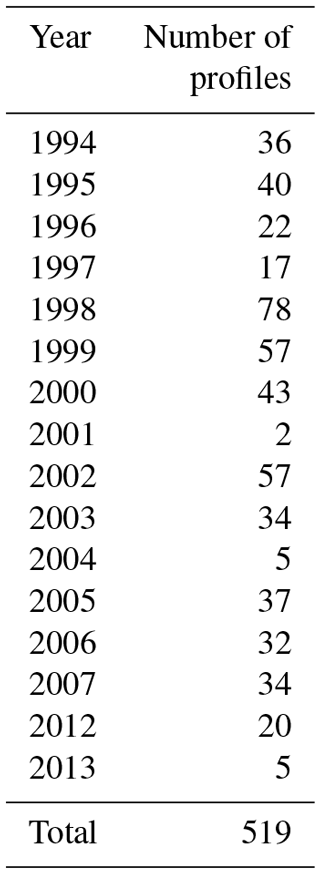
The PCL is a Rayleigh–Raman lidar that was located at the Delaware Observatory (42.52∘ N , 81.23∘ W) near the University of Western Ontario in London, Canada, from 1992 to 2010 (Argall et al., 2000; Sica et al., 1995, 2000). In 2012, the PCL was moved to the Environmental Sciences Western Field Station (43.07∘ N, 81.33∘ W; 275 m of altitude). The PCL has been upgraded over time. Currently, the PCL transmitter is a Nd : YAG laser with a power of 1000 mJ per pulse at 532 nm and a repetition rate of 30 Hz. The PCL receiver is a liquid mercury mirror with a diameter of 2.65 m. From 1994 to 1998, the PCL used a single detection channel (the high-level Rayleigh (HLR) channel) over the range of 30 to 110 km (Sica et al., 1995). In 1999, a low-level Rayleigh (LLR) channel was added, which is nearly linear above 25 km (Sica et al., 2000). This study uses 519 nightly averaged temperature profiles from 1994 to 2013 distributed in time as shown in Tables 1 and 2.
Table 1Number of nightly mean profiles used to calculate the PCL temperature climatology by month between 1994 and 2013.
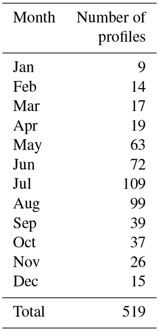
Table 2Number of profiles used to calculate the PCL temperature climatology per year between 1994 and 2013.
2.2 Rayleigh-temperature retrieval methods
In this section, we briefly review the OEM and HC methods that have been used in our calculations. Each approach has its own benefits and deficiencies. Both of these methods start with a lidar return proportional to density and then find temperature using the assumption of hydrostatic equilibrium, the ideal gas law, and the lidar equation.
The lidar equation is a mathematical relation between the number of back-scattered photons detected by lidar and the measurable quantities such as altitude, laser power, and scattering cross section. If we consider all atmospheric parameters in the lidar equation to be constant in time, the lidar equation reduces to Eq. (1):
where C is a constant standing for a combination of all the constant properties of the lidar, ψ(z) includes height-dependent parameters like detector nonlinearities or geometric overlap, n(z) is the atmospheric number density as a function of height, and B(z) is the background count due to radiation sources other than the lidar laser, which may or may not be height dependent.
Various lidar system parameters and physical constants affect the photocounts independent of altitude. The combination of these parameters is called the lidar constant and in our definition includes the number of photons emitted by each laser pulse, the optical efficiency, the detection efficiency of the photomultipliers, atmospheric Rayleigh-scatter cross section, and speed of light. Note that most of these quantities are system dependent, and they in fact can change for a specific instrument as hardware changes, such as changing the laser transmitter. We show in the following sections that the OEM method is robust to these changes and that a consistent climatology can be computed using the OEM.
When the pressure gradient of an air parcel in the atmosphere is in balance with its gravitational force, the atmosphere is in hydrostatic equilibrium and is dynamically and thermally stable. The hydrostatic equilibrium equation can be expressed as
where P is the atmospheric pressure, ρ is the density, and g is the acceleration due to gravity.
The mean molecular mass of air is considered to be constant within the 30 to 80 km altitude range. However, the mean molecular mass varies with altitude above 80 km, and this variation affects the temperature retrieval, both through the change in mean molecular mass and the effect of composition changes on the Rayleigh-scatter cross section.
2.2.1 The HC method
In 1980, Hauchecorne and Chanin presented a robust method to retrieve temperature from Rayleigh lidar measurements (Hauchecorne and Chanin, 1980). The HC method assumes that the atmosphere is comprised of isothermal layers and uses an equation derived from the ideal gas law and the hydrostatic equilibrium assumption to calculate temperature from relative atmospheric density. Using the assumption of hydrostatic equilibrium, the ideal gas law, and the lidar equation, they found a relation between the measured lidar signal and temperature at each altitude in the lidar range. This relation can be integrated from to for a layer with thickness △z as follows:
We can then use the assumption of hydrostatic equilibrium to express the pressure for each layer upon downward integration and derive the following relation for the temperature (Gross et al., 1997):
In order to integrate the pressure relation from top to bottom, a pressure obtained from a model is used to “seed” or to “tie-on” the pressure at the highest altitude of lidar measurements. Due to the high uncertainties caused by the pressure estimation from a model, the top 10 to 15 km are required to be eliminated from the top of each temperature profile to have accurate results (e.g., Khanna et al., 2012). The HC method gives a statistical uncertainty of the calculated temperature, which assumes that the measurements follow Poisson statistics. Khanna et al. (2012) used an inversion approach to retrieve the temperature using a grid search method, and Jalali (2014) applied the grid search method to calculate the PCL temperature climatology and then compared the results with the HC temperature climatology. The grid search is a least-squares approach applied to a nonlinear forward model. The main difference between the grid search method and the OEM is the lack of a regularization term in the grid search forward model. Also, the grid search method uses the Monte Carlo technique to calculate the statistical and seed pressure uncertainties. The grid search method gained 10 km in height over the HC method, but it does not provide the same advantages as the OEM. For example, the grid search method does not provide the full uncertainty budget, vertical resolution, and averaging kernel. Additionally, the grid search method cannot use several channels of measurements to retrieve a single temperature profile, but requires gluing of photocounts or merging temperature profiles, which introduces additional uncertainties that are difficult to quantify.
2.2.2 Optimal estimation theory
Sica and Haefele (2015) used a first-principle OEM to retrieve temperature from Rayleigh-scatter lidar measurements. Here first principle means the forward model is the lidar equation and the measurements to the forward model are the raw (level 0) measurements. The OEM (Rodgers, 2011) solves an inverse problem and uses a forward model to estimate the lidar measurements using a set of input parameters usually referred to as state and model parameters. The inversion of the forward model yields the state vector, while the model parameters are known and the measurement is given.
The forward model (F) can be written as
where y is the measurement vector, x is the state vector, b is the model parameter vector, and ϵ is the measurement noise. The state vector is retrieved and contains the temperature profile and some instrument parameters like detector dead time and background. The model parameter vector contains all other parameters needed to represent the measurements. The forward model is the lidar equation (Eq. 1), which is dependent on both the system hardware configuration and atmospheric properties. The measurement noise in lidar measurements implies that the measurements have uncertainties that have a Gaussian distribution of possible values represented by ϵ. The solution of the inverse problem is constrained around an a priori, which can be found in atmospheric models such as the CIRA-86 model or the US Standard model. CIRA-86 can provide the monthly temperatures for use as the a priori. In its most likely state , the solution is a minimum of a cost function:
where Sϵ is the covariance of the system's state, xa is the a priori vector, and Sa is the the covariance matrix of the system's state.
Unlike the HC method, the OEM produces a complete uncertainty budget for all parameters in the temperature retrieval process on a profile-by-profile basis. The uncertainty budget includes the uncertainty due to the seed pressure and the other model parameters and measurement noise as well as smoothing. A diagnostic variable of the OEM is the averaging kernel, A, a matrix that describes how the retrieval reacts to a given change in the real atmosphere. A perfect retrieval means the retrieved temperature changes in the same way as the real atmosphere and A is equal to the identity matrix (Rodgers, 2011). However, if the contribution of the a priori increases in the temperature retrieval, A drops to <1 at each point for the altitudes at which the a priori has more influence. If u is a vector with unit elements, Au is the sum along the rows of the averaging kernel and it can be used as a representation of the amount of information coming from the lidar measurements and how much is as a result of the a priori. Therefore, Au was used as the cutoff height reference in the OEM instead of removing one or two scale heights from top of each profile as in the traditional method. Values of Au equal to 0.9 and 0.8 are considered as a cutoff height. These values represent the fractional contribution of the measurements compared to the a priori in the temperature retrieval and are generally recognized in the OEM community as levels above which the effect of the a priori is minimal.

Figure 1(a) Temperature difference between the a priori temperature profiles, US Standard Atmosphere, and CIRA-86 (blue line). (b) Temperature difference between the OEM-retrieved temperature profiles using the a priori profile used in Fig. 1a for 24 May 2012 (red line) and the calculated OEM statistical uncertainty (blue line). The solid black and dashed black lines are the height below which the temperature profile is more than 90 % (0.9) and 80 % (0.8) due to the measurements.
2.3 Methodology to calculate temperature climatology
2.3.1 OEM methodology
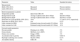
The OEM uses the forward model and non-paralyzable dead time correction equation (Sica and Haefele, 2015) (henceforth SH2015) to retrieve the nightly average temperature profiles from the LLR and HLR channels simultaneously. In SH2015 the dead time, background, and temperature were retrieved. They considered the lidar constant as a forward model parameter, but in this study, the lidar constants for LLR and HLR channels were retrieved rather than specified. The OEM uses an estimation of the covariances of the measurements, retrieval, and forward model parameters. The model parameter covariance matrices used in this study are based on SH2015, in which the summary of the values and related uncertainties of the measurements and the retrieval and forward model parameters are presented in Table 3. The data grid is 264 m, and the retrieval grid is 1056 m. Due to the PCL measurements between 1994 and 1998 having only the HLR channel measurements, temperature and background were retrieved but not dead time. Instead, the systematic uncertainty due to the saturation was calculated. The PCL measurements from 1999 to 2011 used the LLR digital channel to get more temperature information, and the dead time of the HLR channel was retrieved using an a priori value of 10 ns (Table 3). The LLR dead time was treated as a model parameter and a standard deviation of 5.7 % was considered. The CIRA-86 model atmosphere was chosen as the temperature a priori with a variance of (35 K)2 at all altitudes (Fleming et al., 1988).
Fleming et al. (1988)McPeters et al. (2007)Griggs (1968)Mulaire (2000)Nicolet (1984)Table 3Values and associated uncertainties of the measurements and the a priori, retrieval, and forward model parameters
2.3.2 HC methodology
The climatology was formed using the methodology of Argall and Sica (2007) (henceforth AS2007), who used the HC method as follows. First, the quality of each 1 min scan profile of measurements was checked. Then, nightly averaged temperature profiles were calculated. The quality of the nightly averaged measurements was assessed based on the measurement signal-to-noise ratio. Measurements were accepted if the signal-to-noise ratio was greater than 2 at the highest altitude for the initialization of downward integration. AS2007 used the nightly averaged measurements with a minimum signal-to-noise ratio of 2 at the initial height of integration of 95 km; however, this height was reduced to 90 km in this study because the decrease in the initial height of integration led to having more nights, which allowed for a better comparison with the OEM climatology. The raw photon count profiles have been co-added to produce height bins of 1008 m and a “3's and 5's” filter (Hamming, 1989) was applied to the calculated temperature profiles to smooth them in the climatology. The co-added height value of 240 m was chosen as a data grid for the OEM to be consistent with the vertical resolution of the HC. The vertical resolution definition and calculation are based on Leblanc et al. (2016a).
The following steps were taken to make a composite year temperature climatology after calculating all lidar temperature profiles. Only the profiles were used that, after removing the top 10 km, extended up to 80 km. Each temperature profile was then interpolated to an altitude grid with 1 km intervals between 35 and 110 km. For dates with multiple measurements over the years (e.g., 25 July 1994, 2003, and 2003), a weighted-average profile was calculated using each profile's statistical uncertainty as weights. Then, linear interpolation was used to fill the gaps where no measurements existed and a 33-day triangular filter was applied to smooth the composite temperature climatology.
2.4 Effect of a priori on the retrieval temperature profiles in the OEM
A retrieved temperature profile using the CIRA and the US Standard Atmosphere as the a priori for a sample PCL night (24 May 2012) was plotted in order to demonstrate the contribution of the a priori temperature profiles in the retrieval results and the temperature difference between the a priori temperature profiles (Fig. 1). The temperature difference between the a priori profiles is shown in Fig. 1a. The temperature difference around 94 km, which is below the OEM cutoff heights, is about 20 K. In Fig. 1b, the red profile is the temperature difference due to the a priori and the blue profile is the statistical uncertainty calculated by the OEM. The 0.9 and 0.8 value lines in the Au are the cutoff heights for the OEM and are shown with solid and dashed lines, respectively. It can be seen that the choice of a priori has little effect (1.5 K below the 0.9 line and less than 2 K below the 0.8 line) on the retrieved temperature and that the difference between the retrieved temperatures from each choice is much less than the statistical uncertainty (10 K below the 0.9 line and 12 K below the 0.8 line) at the top of the profiles.
To create the temperature climatology, we used the nightly OEM temperature profiles to calculate an average temperature profile for each day of the year (Fig. 2). The 0.9 and 0.8 values of Au are superimposed in Fig. 2 with white lines. To estimate the annual temperature variability, the temperature difference between PCL temperature climatology using the OEM and the calculated climatology from monthly CIRA-86 temperature profiles is plotted in Fig. 3 for each month. There is a temperature difference of the order of 5 K below 52 km. There is a bias smaller than 3 K between the CIRA profiles and the PCL monthly mean temperatures between 55 and 65 km except in the winter. Above 65 km the CIRA is warmer, on average around 8 K, than the PCL up to 90 km, but much colder (of the order of 20 K) above 90 km. CIRA temperature profiles have a smaller difference (less than 10 K) compared to the PCL in summertime rather than wintertime up to around 90 km.

Figure 2Composite PCL Rayleigh-temperature climatology using the OEM. The white lines are the height below which the temperature climatology is more than 90 % (0.9) and 80 % (0.8) due to the measurements.
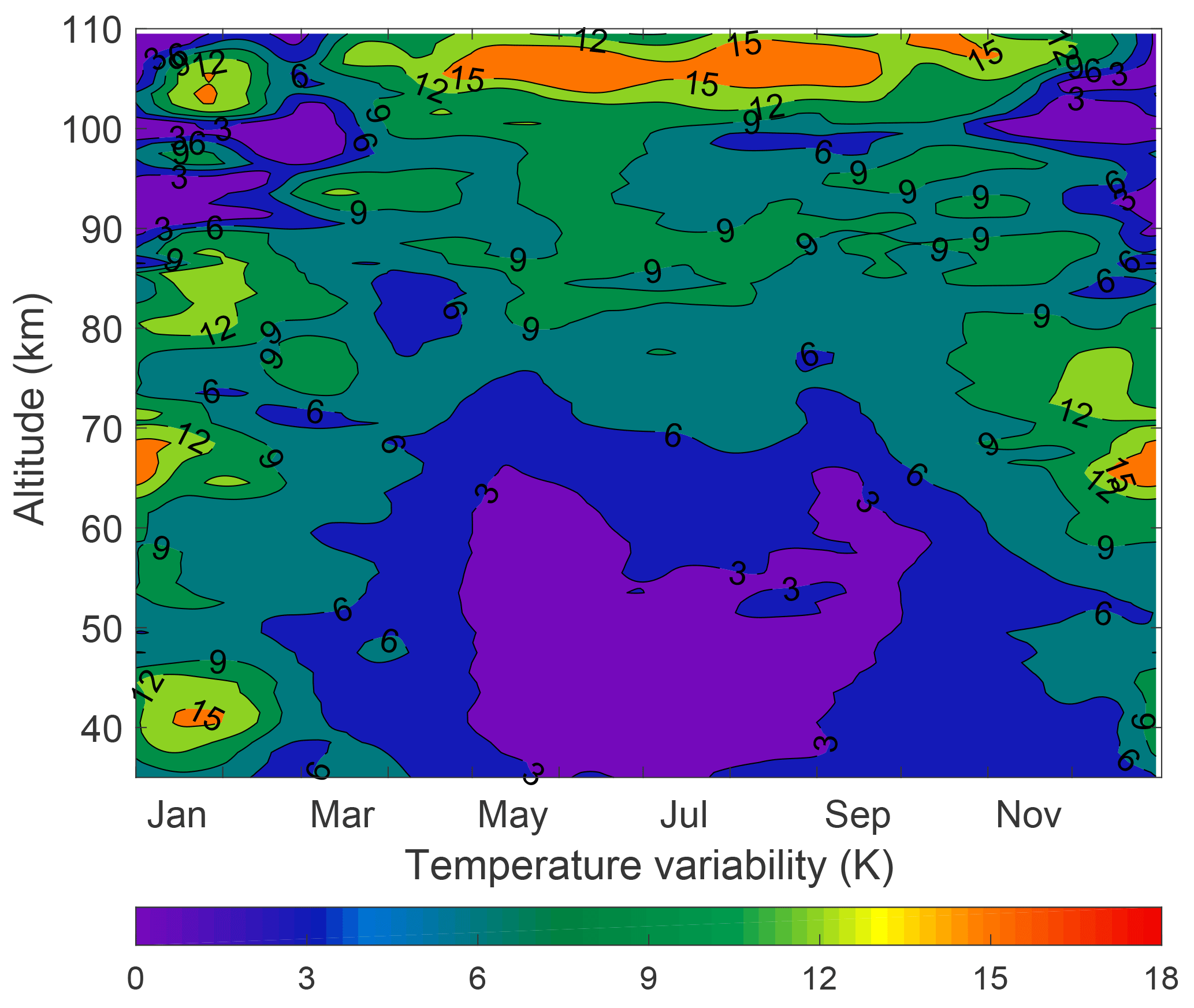
The geophysical variability for the OEM PCL temperature climatology (Fig. 4) was calculated based on the difference between the 33-day temperature standard deviation and the variability of the PCL measurements. The geophysical variability shows the wave activity in the time range of 2 to 33 days, encompassing the scale range of planetary waves. We followed the procedure from AS2007 based on Leblanc et al. (1998) to calculate the geophysical variability. Figure 4 shows the temperature variability related to waves from 2 to 33 days. The temperature variability from mid-April to the end of September below 70 km is less than 4 K. However, in the same period of time the highest temperature change is between 80 and 90 km due to the wave activity in the mesosphere. There is a peak at 41 km in January, which may be related to sudden stratospheric warmings during winter. However, the lower number of measurements in January will also contribute to the variability, and determining the extent of each contribution is not possible (AS2007). The temperature variability due to mesospheric inversion layers reaches a maximum between 62 and 72 km during December and January. These results are in good agreement with the results presented in Fig. 6 of AS2007.
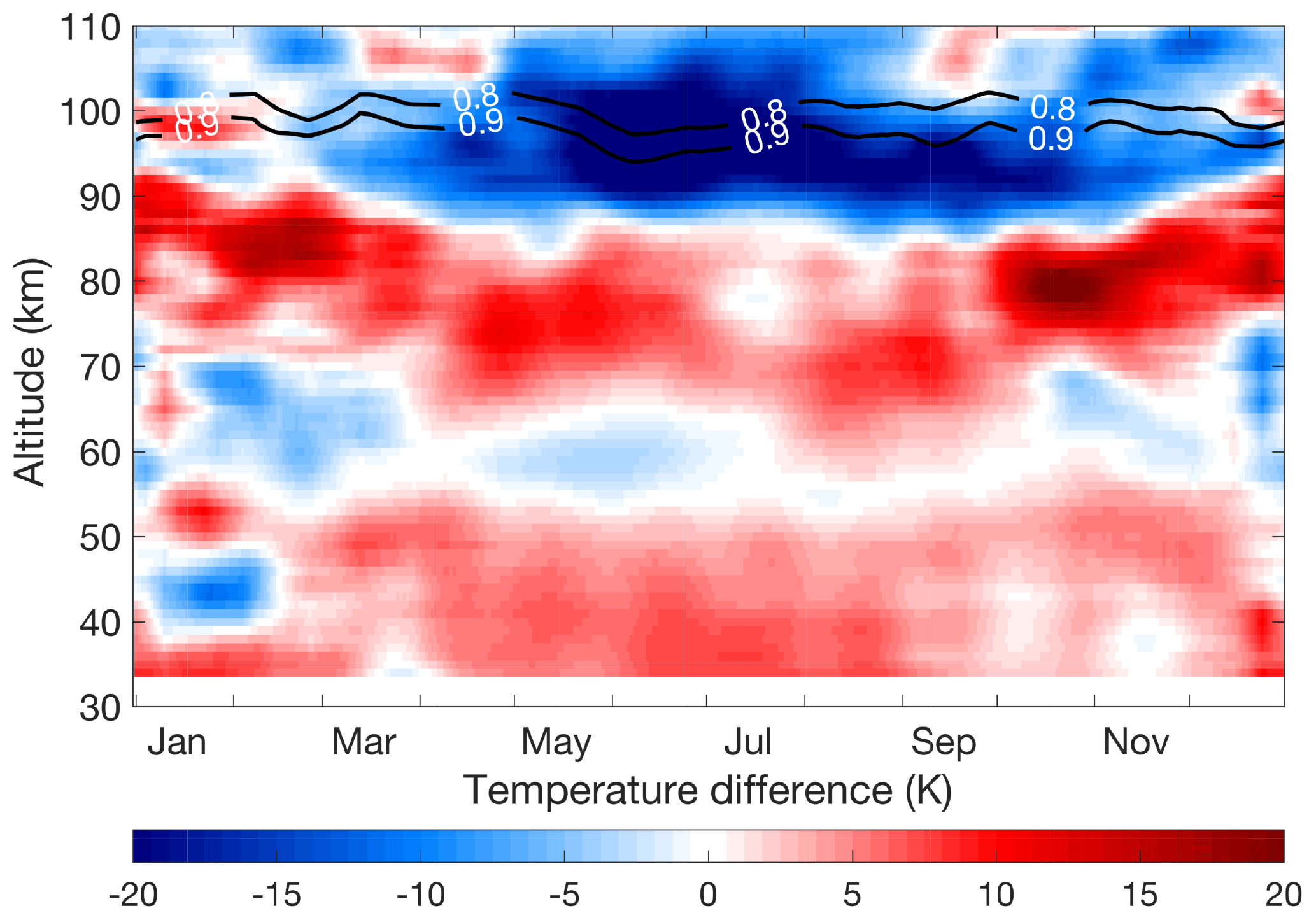
Figure 3Temperature difference between the calculated climatology from monthly CIRA-86 temperature profiles and the OEM PCL temperature climatology (CIRA-86 minus OEM PCL). The black lines are the height below which the temperature climatology is more than 90 % (0.9) and 80 % (0.8) due to the measurements.
3.1 Uncertainty budget and vertical resolution
The lidar measurements include both systematic and random uncertainty. Systematic uncertainties originate in the forward model from uncertainties due to model parameters. One of the advantages of the OEM is that it provides systematic uncertainties for all retrieved parameters, as well as the random uncertainties. The systematic uncertainties calculated in the PCL OEM technique (Table 3) are based on the following model parameters:
-
knowledge of the HLR dead time (1994–1998 only);
-
determination of the Rayleigh-scatter cross section for air;
-
Rayleigh cross section variation with composition in the mesosphere and thermosphere;
-
air number density influence effect on Rayleigh extinction;
-
ozone absorption cross section;
-
ozone concentration effect on transmission;
-
seed (tie-on) pressure;
-
acceleration due to gravity; and
-
mean molecular mass variations with height above 80 km.
3.1.1 Uncertainty budget for the PCL climatology
A typical case for the temperature statistical and systematic uncertainties for a nightly average retrieval is shown in Fig. 5. The temperature uncertainty due to the seed pressure has the highest contribution among all of the systematic uncertainties at the altitudes above the mesopause. However, temperature uncertainties related to ozone, including the ozone absorption cross section, have the largest effect below 40 km. The uncertainty contribution for the gravity model is almost constant with height and is of the order of 0.002 K.

Figure 5A typical night's systematic and random uncertainties for the OEM temperature retrieval.
The nightly OEM statistical uncertainty profiles were used to form the statistical temperature uncertainty of the PCL temperature climatology (Fig. 6) using the procedure described in AS2007. The statistical uncertainty below 75 km is less than 1 K and gradually increases with height until it reaches 0.9 Au at which it is less than 10 K. The monthly average minimum, maximum, and median of temperature uncertainties related to the systematic uncertainties for all months are plotted in Fig. 7.
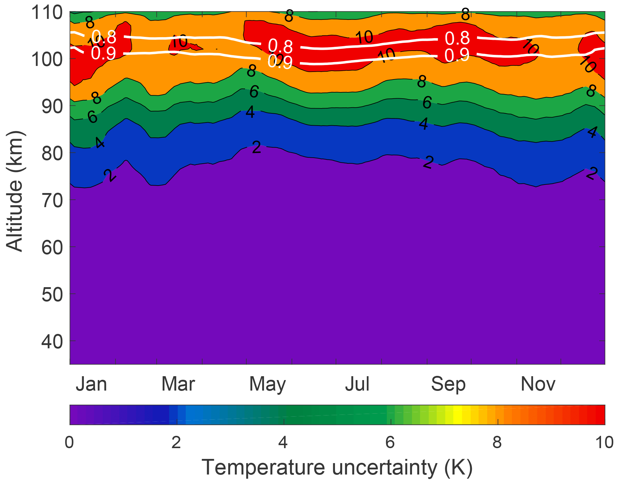
Figure 6Statistical temperature uncertainty of the temperature climatology. The white lines are the height below which the temperature climatology is more than 90 % (0.9) and 80 % (0.8) due to the measurements.
An improvement of the OEM over the HC method is its ability to yield the vertical resolution at each height (Fig. 8). The vertical resolution is 1056 m below 95 km and is equal to the retrieval grid. It is 3000 m below the 0.9 cutoff height; however, it increases rapidly to 5000 m around the 0.8 cutoff line. Leblanc et al. (2016b) recommended two standardized definitions for a temperature profile vertical resolution. In order to compare the retrieved temperature profiles using the OEM and the HC method, the two vertical resolution definitions given by Leblanc et al. (2016b) were used to find the best bin size for the HC method so it would have an identical vertical resolution to the OEM retrieval. We found that 264 m co-added bins and a “3's and 5's” filter gave a vertical resolution of 1008 m, close to the OEM temperature retrieval grid (1056 m).

Figure 7PCL temperature systematic uncertainty due to the (a) saturation function (1994 to 1998 only), (b) Rayleigh extinction cross section, (c) Rayleigh cross section variation with height, (d) air density affect on Rayleigh extinction, (e) ozone absorption cross section (f) ozone concentration, (g) seed (tie-on) pressure, (h) gravity model, and (i) mean molecular mass variation with height. In each figure, red, blue, and black lines are the minimum, maximum, and median between all months, respectively.
3.1.2 Comparison with uncertainty budget of the traditional method
Leblanc et al. (2016b), hereafter NDACC2016, used a Monte Carlo method to calculate the statistical and systematic uncertainties for the temperature retrieval. We have compared our results with his ND : YAG 532 nm lidar results. NDACC2016 and our climatology give the temperature uncertainties for several of the same parameters (Table 3), including the statistical uncertainty (detection noise), the Rayleigh cross section, air number density, ozone absorption cross section, ozone number density, and the gravity model. NDACC2016 calculated the temperature uncertainty due to each parameter per 1 % uncertainty. In order to compare NDACC2016 results with the PCL uncertainties using the OEM, we need to scale NDACC2016 simulations to the PCL as recommended by Leblanc et al. (2016b). For example, if the temperature uncertainty due to air number density is per 1 % uncertainty in NDACC2016, then we must multiply NDACC2016 uncertainties by a factor of 5 because we assume an air number density uncertainty of 5 % (recommended by NDACC2016) in the PCL forward model (Table 3). We have compared our results with the statistical and systematic uncertainties presented in Figs. 1 to 9 in NDACC2016 for the case of a 532 nm laser beam with a 1 MHz count rate at 45 km, a height resolution of 300 m, and an integration time of 2 h (Fig. 9).
The statistical uncertainty comparison between the PCL and NDACC2016 is shown in dark blue in Fig. 9. It can be seen that the NDACC2016 statistical uncertainty almost equals the scaled PCL statistical uncertainty above the stratopause. However, there is a difference at altitudes below 50 km. The statistical uncertainty difference in the lower altitudes is due to using the two Rayleigh channel measurements (HLR and LLR) to calculate the temperature in the lower altitudes. The uncertainties at these altitudes are then a combination of the LLR and HLR uncertainties.
The temperature uncertainty due to the uncertainty in the Rayleigh cross section in NDACC2016 for each 1 % at two sample altitudes, 30 and 38 km, is of the order of 0.001 K (NDACC2016, Fig. 4). The temperature uncertainty due to the Rayleigh cross section in the OEM is presented per 0.2 %; therefore, the scaled cross section uncertainty for NDACC2016 is 1 order of magnitude smaller than the PCL Rayleigh cross section uncertainty. However, this temperature uncertainty is very small.
The uncertainty due to air number density as an input quantity per 1 % is shown in NDACC2016 (their Fig. 5 left panel). The NDACC2016 scaled temperature uncertainty due to air number density is of the same order of magnitude as the OEM-derived uncertainty for the PCL (Fig. 9).
The standard deviation for the ozone cross section in the OEM forward model is 2 %. Therefore, the NDACC2016 ozone cross section temperature uncertainties should be doubled to compare them with the PCL. The temperature uncertainty due to the ozone cross section uncertainty in NDACC2016 (their Fig. 6a) after scaling is about 4 times smaller. The other temperature uncertainty due to ozone is the ozone number density. The temperature uncertainty due to ozone number density uncertainty for the NDACC (their Fig. 7a), after scaling by a factor of 0.25 (as the PCL a priori assumes 4 % uncertainty), is almost twice that of the PCL's. The uncertainties due to ozone number density are so small above 45 km that they have not been listed in the total uncertainty budget in NDACC2016's final results.
The temperature uncertainty due to the choice of pressure at the highest altitude (seed pressure) is called the tie-on uncertainty in NDACC2016. The tie-on uncertainties are in the same range and the small differences between the PCL and NDACC2016 (their Fig. 8) are related to the fact that the seed pressure altitude is at 99 km for NDACC2016 and at 110 km for the PCL.
The gravity temperature uncertainties for both NDACC2016 and the scaled PCL are consistent and are roughly 0.002 K. NDACC2016 states that the temperature uncertainty due to the molecular mass is negligible below 85 km and is of the order of 0.05 K and above 85 km can increase up to 1 K (NDACC2016, Table 3). The OEM shows that the PCL molecular mass temperature uncertainty at 85 km is 0.06 K. The PCL molecular mass temperature uncertainties from 90 to 100 km are between 0.1 and 0.6 K. However, the semi-empirical mean molecular mass variation of the US Standard model is considerably different from the variation assumed by NDACC2016, accounting for the differences in the calculated uncertainties.
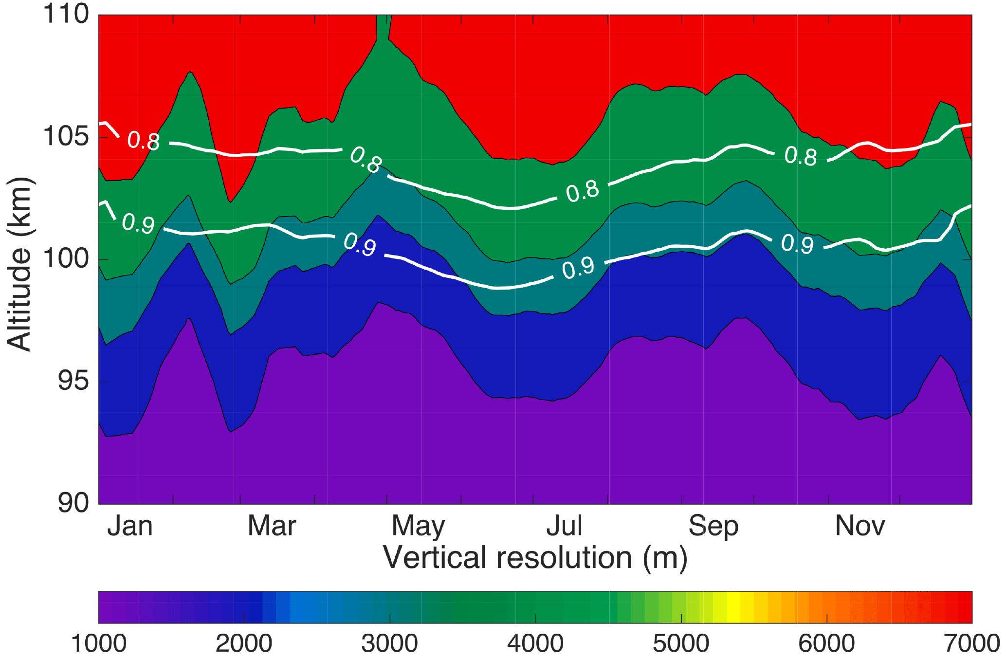
Figure 8The OEM vertical resolution. The vertical resolution below 80 km is 1056 m; that is, it is equal to the retrieval grid spacing (not shown). The white lines are the height below which the temperature climatology is more than 90 % (0.9) and 80 % (0.8) due to the measurements.
In order to evaluate the OEM results, the new OEM PCL temperature climatology was compared with the existing PCL temperature climatology using the HC method, as well as other climatologies including sodium lidar climatologies.
4.1 Comparison between the PCL climatology using the OEM and HC methods
AS2007 used PCL measurements between 1994 and 2004 to calculate a PCL temperature climatology (henceforth, 2004 PCL climatology) using the HC method. The top 10 km of all temperature profiles was removed from the 2004 PCL climatology in order to reduce the effect of seed pressure and the same procedure was followed in the HC calculations for the updated PCL climatology (between 1994 and 2013). The temperature differences between the OEM and updated HC PCL temperature climatologies are shown in Fig. 10. The white space in the upper part of Fig. 10 is due to removing 10 km from the top of each profile for the updated HC PCL climatology. In addition, the lines corresponding to the 10 and 15 km cutoff for the HC method and the 0.9 cutoff line for the OEM are superimposed onto Fig. 10.
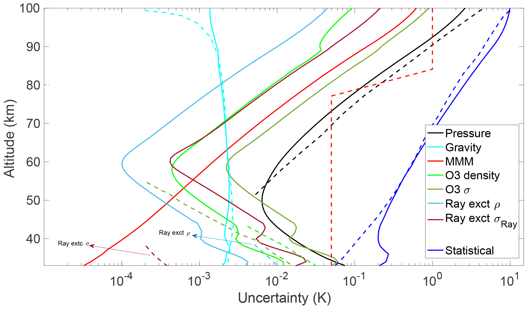
Figure 9Comparison of the PCL statistical and systematic uncertainties with scaled uncertainties from Leblanc et al. (2016b) as described in the text. The solid lines are the uncertainties due to the PCL and the dashed lines are uncertainties due to NDACC2016.
The OEM temperature climatology is 0.55±0.23 K warmer than the updated HC climatology average from 40 to 60 km. Although the difference is within the statistical uncertainty of the measurements (Fig. 5), there is a warm bias. The bias due to differences in ozone profile between the two climatologies is only +0.05 K. The OEM used measurements from two Rayleigh channels (HLR and LLR) after 1999 to calculate the OEM climatology, while only the HLR channel measurements were used for the HC method and the OEM before 1999. The effective LLR signal is up to about 60 km of altitude. The temperature difference in the bottom range (between 40 and 60 km) of measurements is because of using a two-channel retrieval in the OEM and comparing it with a one-channel (HLR) retrieval in the HC method. The two-channel OEM method retrieves the dead time for each profile, while the dead time in the HC method was an empirically determined constant based on count measurements using a pulsed LED source. In order to compare the OEM with HC temperature climatology, we could have merged the calculated LLR and HLR temperature profiles in the HC method. However, the temperature uncertainty induced by the merging will be more than the ±0.05 K temperature difference between the OEM and HC climatology (Jalali, 2014).
The OEM temperature above 80 km up to the 10 and 15 km cutoffs is colder than the temperatures obtained using the HC method. The temperature differences above 80 km are mostly due to the sensitivity of the model seed pressure in the HC method. Figure 10 shows that the OEM temperature climatology reaches 5 to 10 km higher in altitude than the HC temperature climatology. The differences between the OEM and HLR are not calculated below 40 km due to the lack of HLR data in some time periods.
Finally, in order to evaluate the effect of the a priori on the temperature differences, the same temperature climatologies were calculated using the OEM with the US Standard model as the a priori temperature profile and the same differences as discussed above were obtained, again demonstrating that the results show little sensitivity to the choice of any reasonable a priori profile.

Figure 10PCL temperature climatology difference between the OEM and HC method (OEM minus HC) using seed pressure. The blue lines show the height below which the OEM temperature climatology is more than 90 % (0.9) and 80 % (0.8) due to the measurements. The red lines are the 10 and 15 km cutoff height for the HC method.
The HC method usually uses a seed pressure value at the highest point of the profile. However, the seed pressure can be substituted by temperature and density and is called the seed temperature (Gardner et al., 1989, Eq. 86). When a seed temperature is used, the temperature is obtained from the CIRA-86 model, and the measured relative density profile is normalized (typically by a model) to obtain a seed pressure to use in the HC retrieval. The temperature differences between the OEM climatology and the updated HC climatology using the seed temperature (instead of seed pressure) are shown in Fig. 11. Comparing Figs. 10 and 11 reveals that the temperature difference above 80 km between the OEM and the updated HC using seed temperatures is larger than the differences between the OEM and the updated HC using seed pressures. However, the differences below 80 km are identical and the small temperature differences between the OEM and HC method are due to the tie-on temperature or pressure value. The difference between the HC climatologies calculated by these two methods highlights the sensitivity to seed pressure at the greatest heights in this method.
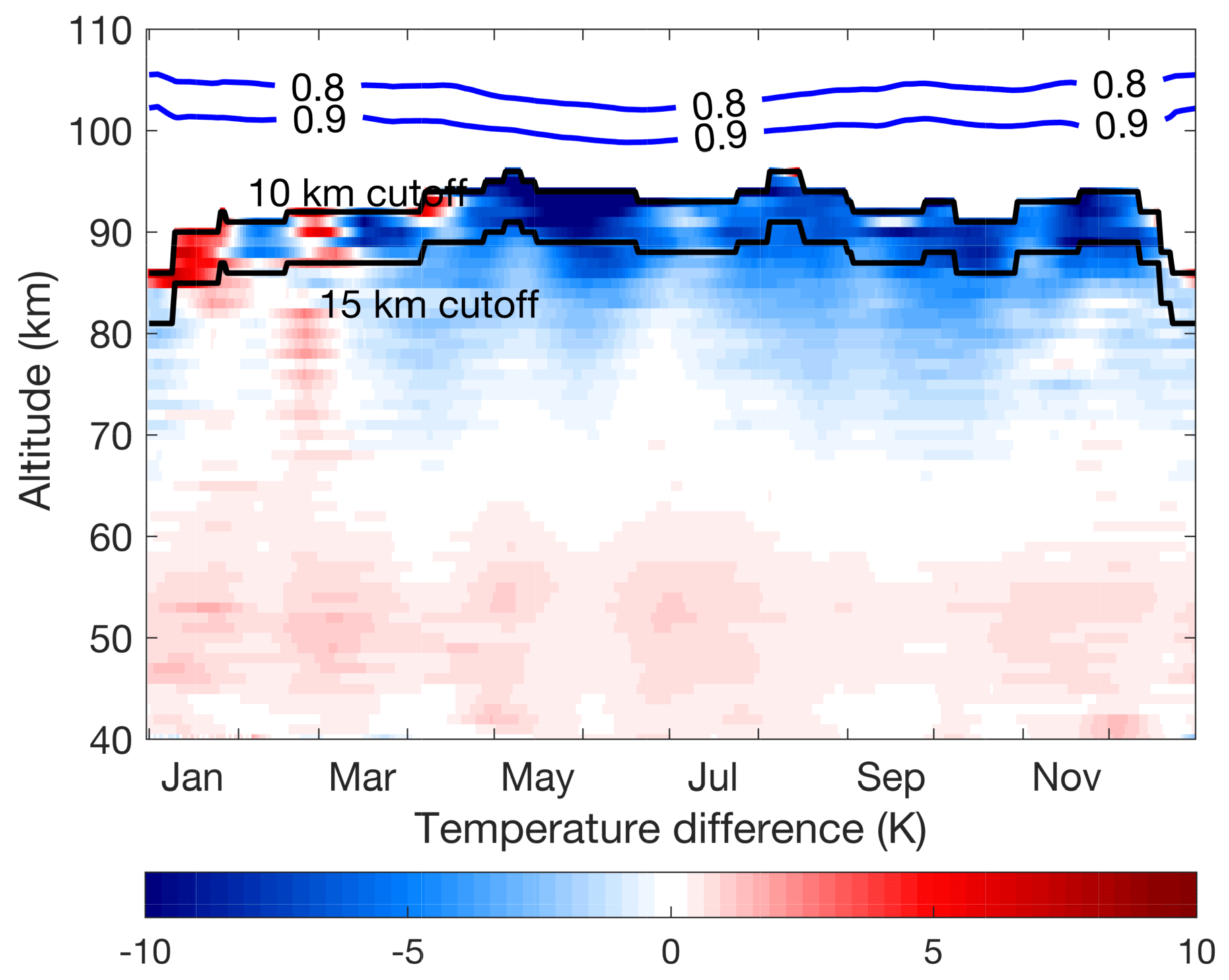
Figure 11PCL temperature climatology difference using the OEM and HC method (OEM minus HC) using seed temperature. The blue lines show the height below which the OEM temperature climatology is more than 90 % (0.9) and 80 % (0.8) due to the measurements. The black lines are the 10 and 15 km cutoff height for the HC method.
Gerding et al. (2008) used coincident Rayleigh and sodium resonance lidar temperature measurements to minimize the seed pressure. For altitudes below the sodium layer, Rayleigh lidar measurements are used to determine the temperature. While having this combination of a Rayleigh and resonance temperature lidar is ideal, most Rayleigh-temperature lidar systems are not colocated with a resonance temperature lidar, and hence the effect of seed pressure is the largest systematic uncertainty at the upper range of the temperature profile determined.
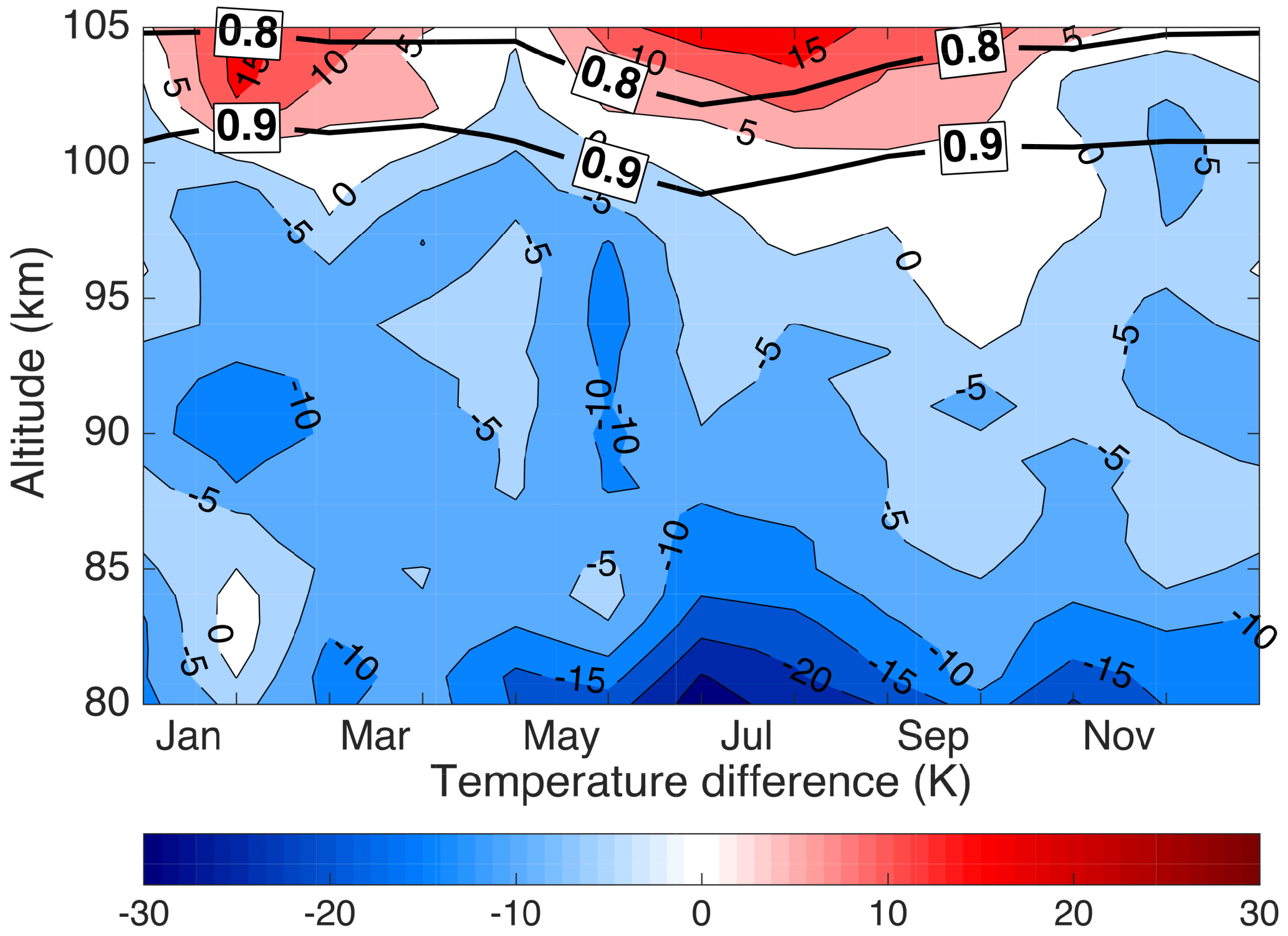
Figure 12PCL temperature climatology difference from the URB sodium lidar climatology (PCL minus URB). The horizontal black lines are the height below which the temperature climatology is more than 90 % (0.9) and 80 % (0.8) due to the measurements.
4.2 Comparison with sodium lidar climatologies
The comparison between the PCL Rayleigh-temperature climatology using the HC method with sodium lidars was done by AS2007. Their results showed that the average temperature between 83 and 95 km measured by the PCL was between 7 and 7.4 K colder than CSU and URB climatologies, respectively. Using the OEM to extend the PCL Rayleigh lidar temperature climatology to above 100 km provides the opportunity to validate the PCL results against sodium lidar climatologies, which have their highest signal-to-noise ratio in a few kilometer-wide regions between about 90 and 95 km of altitude, and obtain sufficient high-quality measurements to calculate climatologies from 85 to 105 km. Sodium lidars directly measure the kinetic temperature without assuming hydrostatic equilibrium or requiring the knowledge of mean molecular mass and molecular cross section variations with height and can be configured to obtain temperatures during both the day and night. She et al. (2000), Yuan et al. (2008), and States and Gardner (2000a) have published sodium temperature lidar climatologies in the same latitude range as PCL. Both sites are west of the PCL, but in the case of URB the separation in longitude is less than 8∘. The URB and CSU climatologies are among the best datasets for validation of upper-mesosphere and lower-thermosphere temperatures, plus they allow for a direct comparison between our new climatology and AS2007. The upgraded CSU (Yuan et al., 2008) provides additional years of overlap with our new climatology for validation of our OEM-derived temperatures. The nighttime URB and upgraded CSU temperature climatologies were compared with the PCL temperature climatology.

Figure 13PCL temperature climatology difference from the CSU (1990–1999) sodium lidar climatology (PCL minus CSU). The horizontal black lines are the height below which the temperature climatology is more than 90 % (0.9) and 80 % (0.8) due to the measurements.
The PCL temperature climatology differences using the OEM compared with the sodium lidars are presented in Figs. 12, 13, and 14. The absolute value of the average differences in 5 km height bins between the sodium lidar temperature climatologies and the PCL climatology using the OEM and the HC method are given in Table 4. The absolute value is used to avoid differences canceling each other. The bottom part of the table is important, as it gives the differences between the sodium lidars themselves. The differences between the sodium lidars are taken as the level of difference defining the agreement between the PCL lidar and the sodium systems. The PCL HC climatology in general does not agree with the sodium lidar climatologies to the same extent to which they agree with each other, while the PCL OEM climatology typically does agree with the sodium lidar climatologies to the level at which they agree with each other. The temperature differences between the PCL OEM and sodium lidar climatologies for the entire range of altitudes (80 to 105 km) are smaller than the temperature difference between the PCL HC climatology and the sodium lidar climatologies in the range of 80 to 95 km for which PCL HC temperatures are available. There is a temperature difference at the winter mesopause between the PCL climatology and CSU climatology, but this difference has decreased in the upgraded nighttime CSU climatology compared to that determined by AS2007. The large temperature differences between the PCL (OEM) and URB temperature climatology during summertime below 85 km existed in AS2007 and may be in part due to the signal-to-noise ratio of the sodium lidar measurements rapidly decreasing below 85 km.
Table 4Absolute value of the average PCL temperature differences with sodium lidars and the temperature difference between sodium lidars. The HC method does not provide the temperature above 95 km; therefore, the columns with an altitude range greater than 95 km are shown as “–”.
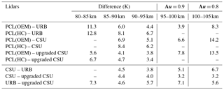
Overall comparisons between the PCL climatologies and sodium lidar climatologies (Table 4) show that in the 85–90 km and 90–95 km height ranges, at which both the Rayleigh and Na methods have good measurement signal-to-noise ratio, the OEM-calculated temperatures show 20 % better agreement with the sodium lidars than the HC method temperatures: that is, 5.0 K versus 6.3 K on average. The variability of the temperature difference between the sodium lidars themselves is around 4.5 K. The difference among the sodium lidars is approximately the same as the differences with the OEM-derived temperatures, meaning the temperatures derived using the OEM retrieval are approximately the same as those from the sodium lidars; this is contrary to the AS2007 comparison, which showed significant differences between the two techniques. Furthermore, the OEM temperature retrievals allow valid retrievals to be obtained in the 95–100 km altitude region, where the systematic uncertainty of the tie-on pressure of the HC-derived temperatures is too large for the temperatures to be useful. Possible sources of these differences were addressed in AS2007, but they did not have the uncertainty budget now available to assess systematic uncertainties. These differences could include the following factors.

Figure 14PCL temperature climatology difference from the upgraded CSU (2002–2006) sodium lidar climatology (PCL minus upgraded CSU). The horizontal black lines are the height below which the temperature climatology is more than 90 % (0.9) and 80 % (0.8) due to the measurements.
-
The assumption of a seed pressure can introduce uncertainty in the PCL temperature retrievals. Using an OEM allows us to calculate the effect of this assumption quantitatively (Fig. 7). In the altitude range of 80 to 95 km, it is less than 1.5 K, increasing to a maximum of 3.5 K at 100 km.
-
The effects of Rayleigh-scatter cross section, Rayleigh-scatter density, and mean molecular mass were mentioned in AS2007 as possible reasons for discrepancies with the sodium lidar temperatures. Figure 7 shows a quantitative determination of the magnitude of these effects. The uncertainties for the Rayleigh-scatter cross section and Rayleigh-scatter density are much less than the temperature differences between the two measurement techniques. Mean molecular mass uncertainty is larger than the other two parameters, but its maximum value is less than 0.7 K at 105 km.
-
The other significant contribution to the temperature uncertainty budget at higher altitudes is ozone cross section, whose uncertainty increases with altitude due to increasing measurement uncertainty (as do many of the retrieval uncertainties due to the model parameters). The uncertainty on the retrieved temperatures due to ozone reaches a maximum of 1 K at 100 km.
-
Geographic location could be another possible cause. The PCL is about 3∘ north of the sodium lidars and, while relatively close to URB in longitude, the PCL is 24∘ east of CSU. Hence, tides and planetary waves could be the primary cause of the temperature differences between the PCL, URB, and CSU lidars. Gravity waves could also contribute, although the effect of gravity waves is minimized by averaging temperature over several hours and using common days in different years to calculate the composite climatology. Sica and Argall (2007) have shown that the seasonal gravity wave activity over London, Canada, is large and highly variable and is possibly related to London's proximity to both Lake Ontario to the west and Lake Erie to the east. The effect of solar tides on the sodium lidar temperature is discussed in States and Gardner (2000b) and Yuan et al. (2006). The upgraded CSU is capable of continuous observation during day and night. Yuan et al. (2008) removed tidal signals from the mean values and calculated diurnal mean monthly temperatures. They show that the amplitude of the diurnal tide is around 5 K at night between 84 and 95 km, increasing to 8 K at 100 km. Hence, we conclude that large-scale waves cause many of the discrepancies between locations.
The comparison with sodium lidars shows that the PCL Rayleigh-temperature climatology using the OEM in general agrees as well with the sodium lidar climatologies as the sodium climatologies agree with one another, validating the PCL OEM height-extended climatology.
Here we have confirmed the validity of using the OEM to retrieve Rayleigh-scatter lidar temperatures on a long-term measurement set. The results of our investigation using the OEM on 519 nights of measurements are summarized as follows.
-
Our OEM can estimate a valid cutoff height at which the entire temperature profile below that level depends less than a specified level on the choice of the a priori temperature profile. Based on best practice in the OEM community, we suggest using measurements whose summed averaging kernels at a retrieval altitude are greater than 0.9.
-
The effect of the temperature a priori on the OEM result was evaluated using the CIRA-86 and US Standard model. It was shown that the effect of the a priori is much smaller than the statistical uncertainty below the OEM cutoff heights for the PCL.
-
We presented a full uncertainty budget for our climatology, which includes both random and systematic uncertainties, including the systematic uncertainty for nine model parameters including mean molecular mass, Rayleigh cross section, Rayleigh cross section variation with composition, seed pressure, air number density (for extinction), ozone absorption cross section, ozone density, and acceleration due to gravity. This uncertainty budget is available on a profile-by-profile basis.
-
The PCL uncertainties were compared to the uncertainty budget simulations presented by Leblanc et al. (2016b). The comparison shows in general similar orders of magnitude, except for the Rayleigh-scatter cross section, which has a larger difference but makes a very small (0.001 K) contribution to the uncertainty budget.
-
Our OEM computes the vertical resolution of each temperature profile. The vertical resolution is equal to the retrieval grid (1056 m) until about 75 km, at which it starts to increase and is about 3 km around the 0.9 cutoff height.
-
The PCL temperature climatology is calculated using both the OEM and the HC method. By 15 km below the cutoff height, any differences in the temperature are within the statistical uncertainty at those heights. Our OEM retrieval determines temperature profiles, which reach 5 to 10 km higher than the temperature profiles calculated by the HC method due to the OEM's ability to evaluate the effect of seed pressure on the retrieved temperature.
-
The temperature difference between the OEM PCL temperature climatology with the HC method PCL climatology using seed pressure was smaller than the temperature difference between the OEM PCL temperature climatology with the HC method temperature climatology using seed temperature. Hence, we recommend that when using the HC method it is better to take the seed pressure from the model than a seed temperature.
-
The PCL temperature climatology is compared with three other sodium lidar climatologies. The temperature differences between the PCL climatology using the OEM and the sodium lidar climatologies are smaller by 1 K than the differences between the PCL–OEM and the PCL–HC differences. The temperature differences between the PCL–OEM and the sodium lidars are within the temperature differences between the sodium lidars themselves (Table 4). The OEM provides the PCL temperature profiles to higher altitudes and these profiles show smaller differences with the sodium lidars than the HC method; thus, using the OEM improves the climatology between 80 and 100 km, as validated by the sodium lidar measurements.
-
The statistical uncertainty of the sodium lidar temperatures is lowest in the 95±5 km region of the peak of the sodium layer. Here the precision is about 1 K to 2 K (Papen et al., 1995). The accuracy of the measurement in this region has been studied in detail by Krueger et al. (2015), who obtain an accuracy of 1 to 2.5 K. The statistical uncertainty increases rapidly away from the sodium layer peak. The closest agreement between the PCL temperature climatology and the sodium lidars' climatology is in the range of 85 to 100 km, with larger temperature differences below 85 km and above 100 km at which the sodium density is lowest. The URB climatology, which was obtained from a station much closer in longitude to the PCL, shows better agreement than the CSU measurements, although all three sodium lidar climatologies have overall good agreement with the PCL OEM climatology. Overall the OEM provides closer temperature results to the sodium lidars than the HC method at all heights and allows the climatology to extend to a greater altitude.
We have shown that using the OEM to retrieve temperature from Rayleigh-scatter lidar measurements has significant advantages over the traditional method, and the advantages shown in our initial study for a small number of nights is practical for a large dataset. These advantages include the ability to calculate a full uncertainty budget on a profile-by-profile basis, determination of the vertical resolution, and the availability of averaging kernels. Applying the OEM will help in the standardization of the uncertainty budget and vertical resolution calculations for comparisons between lidars, as well as comparisons among other instruments with differing vertical resolutions.
We found that a cutoff height of Au = 0.9 is a good estimate for a cutoff height of the retrieval based on the comparison with the sodium lidars. It would be recommended to use the 0.9 height cutoff to minimize the effect of the a priori on the temperature retrieval while keeping the a priori effect on the temperature retrieval less than the statistical uncertainty.
Sodium lidars are well characterized and make the best temperature measurements in the mesosphere and lower thermosphere for validation of the PCL temperature climatology, particularly as the URB and CSU systems are relatively near the PCL. The agreement between the OEM-based PCL climatology and the sodium lidars has improved over the traditional method, and the agreement between the PCL and the sodium lidars is typically as good as the agreement between the sodium lidars themselves. Much of the variability seen in the measurements made at the different locations is likely due to tides and planetary waves.
We hope the results of this study encourage other Rayleigh lidar groups to process their measurements using our OEM retrieval method.
The PCL is a member of the NDACC network, and the temperature measurements in this paper are in the process of being submitted. The data will be available publicly through the NDACC website at ftp://ftp.cpc.ncep.noaa.gov/ndacc/station/londonca/hdf/(Sica, 2018).
AJ was responsible for the data analysis, developing the code to form the climatologies, and paper preparation. He was also involved in operating the lidar after July 2012. This work forms part of his doctoral thesis. RJS was responsible for the supervision of the doctoral thesis, contributions to paper preparation, coding the OEM temperature retrieval, and, in collaboration with AH, first applying the OEM to Rayleigh lidar temperature retrievals. AH contributed to paper preparation and many OEM and scientific discussions relevant to this work.
The authors declare that they have no conflict of interest.
This project has been funded in part by Discovery Grants and a CREATE
Training Program in Arctic Atmospheric Science (PI Kimberly Strong) from the National Science and Engineering
Research Council of Canada and awards from the Canadian Foundation for
Climate and Atmospheric Science. We would like to thank the Federal Office of
Meteorology and Climatology, MeteoSwiss, for its support of this project.
Ali Jalali would like to thank Shannon Hicks-Jalali for her comments and
suggestions on the paper. We would like to thank Stephen Argall for his
many contributions to the PCL lidar program and Tao Yuan for providing to
us in a digital format the upgraded CSU nighttime sodium temperature
climatology.
Edited by:
Gerd Baumgarten
Reviewed by: four anonymous referees
Argall, P. S. and Sica, R. J.: A comparison of Rayleigh and sodium lidar temperature climatologies, Ann. Geophys., 25, 27–35, https://doi.org/10.5194/angeo-25-27-2007, 2007. a, b, c
Argall, P. S., Vassiliev, O. N., Sica, R. J., and Mwangi, M. M.: Lidar measurements taken with a large-aperture liquid mirror: 2. The Sodium resonance-fluorescence system, Appl. Optics, 39, 2393–2399, 2000. a
Arnold, K. S. and She, C. Y.: Metal fluorescence lidar (light detection and ranging) and the middle atmosphere, Contemp. Phys., 44, 35–49, 2003. a
Bills, R. E., Gardner, C. S., and She, C. Y.: Narrow band lidar technique for sodium temperature and Doppler wind observations of the upper atmosphere, Opt. Eng., 30, 13–21, 1991. a
Fleming, E. L., Chandra, S., Shoeberl, M. R., and Barnett, J. J.: Monthly Mean Global Climatology of Temperature, Wind, Geopotential Height and Pressure for 0–120 km, NASA Tech. Memo., NASA TM100697, 85 pp., 1988. a, b
Gardner, C. S., Senft, D. C., Beatty, T. J., Bills, R. E., and Hostetler, C. A.: Rayleigh and sodium lidar techniques for measuring middle atmosphere density, temperature, and wind perturbations and their spectra, in: World Ionosphere/Thermosphere Study Handbook, 2, 141–187, 1989. a
Gerding, M., Höffner, J., Lautenbach, J., Rauthe, M., and Lübken, F.-J.: Seasonal variation of nocturnal temperatures between 1 and 105 km altitude at 54∘ N observed by lidar, Atmos. Chem. Phys., 8, 7465–7482, https://doi.org/10.5194/acp-8-7465-2008, 2008. a
Griggs, M.: Absorption coefficients of ozone in the ultraviolet and visible regions, J. Chem. Phys., 49, 857–859, 1968. a
Gross, M. R., McGee, T. J., Ferrare, R. A., Singh, U. N., and Kimvilakani, P.: Temperature measurements made with a combined Rayleigh–Mie and Raman lidar, Appl. Optics, 36, 5987–5995, 1997. a
Hamming, R. W.: Digital Filters, Prentice Hall, Englewood Cliffs, New Jersey, 3rd Edn., 1989. a
Hauchecorne, A. and Chanin, M.: Density and temperature profiles obtained by lidar between 35 and 70 km , Geophys. Res. Lett., 7, 565–568, 1980. a, b
Hauchecorne, A., Chanin, M.-L., and Keckhut, P.: Climatology and trends of the middle atmospheric temperature (33–87 km) as seen by Rayleigh lidar over the south of France, J. Geophys.Res.-Atmos., 96, 15297–15309, 1991. a
Jalali, A.: Extending and Merging the Purple Crow Lidar Temperature Rayleigh and Vibrational Raman Climatologies, Master's thesis, the University of Western Ontario, Electronic Thesis and Dissertation Repository, 2490, available at: https://ir.lib.uwo.ca/etd/2490, 2014. a, b
Khanna, J., Bandoro, J., Sica, R. J., and McElroy, C. T.: New technique for retrieval of atmospheric temperature profiles from Rayleigh-scatter lidar measurements using nonlinear inversion, Appl. Optics, 51, 7945–52, 2012. a, b
Krueger, D. A., She, C.-Y., and Yuan, T.: Retrieving mesopause temperature and line-of-sight wind from full-diurnal-cycle Na lidar observations, Appl. Optics, 54, 9469–9489, 2015. a, b
Leblanc, T., McDermid, I. S., Keckhut, P., Hauchecorne, A., She, C. Y., and Krueger, D. A.: Temperature climatology of the middle atmosphere from long-term lidar measurements at middle and low latitudes, J. Geophys. Res.-Atmos., 103, 17191–17204, 1998. a, b, c
Leblanc, T., Sica, R. J., van Gijsel, J. A. E., Godin-Beekmann, S., Haefele, A., Trickl, T., Payen, G., and Gabarrot, F.: Proposed standardized definitions for vertical resolution and uncertainty in the NDACC lidar ozone and temperature algorithms – Part 1: Vertical resolution, Atmos. Meas. Tech., 9, 4029–4049, https://doi.org/10.5194/amt-9-4029-2016, 2016a. a
Leblanc, T., Sica, R. J., van Gijsel, J. A. E., Haefele, A., Payen, G., and Liberti, G.: Proposed standardized definitions for vertical resolution and uncertainty in the NDACC lidar ozone and temperature algorithms – Part 3: Temperature uncertainty budget, Atmos. Meas. Tech., 9, 4079–4101, https://doi.org/10.5194/amt-9-4079-2016, 2016b. a, b, c, d, e, f
McPeters, R. D., Labow, G. J., and Logan, J. A.: Ozone climatological profiles for satellite retrieval algorithms, J. Geophys. Res.-Atmos., 112, D05308, https://doi.org/10.1029/2005JD006823, 2007. a
Mulaire, W.: Department of Defense World Geodetic System 1984, Its definition and relationship with local geodetic systems, NIMA TR8350.2, 1–175, 2000. a
Nicolet, M.: On the molecular scattering in the terrestrial atmosphere: an empirical formula for its calculation in the homosphere, Planet. Space Sci., 32, 1467–1468, 1984. a
Papen, G. C., Pfenninger, W. M., and Simonich, D. M.: Sensitivity analysis of Na narrowband wind–temperature lidar systems, Appl. Optics, 34, 480–498, 1995. a
Ramaswamy, V., Chanin, M.-L., Angell, J., Barnett, J., Gaffen, D., Gelman, M., Keckhut, P., Koshelkov, Y., Labitzke, K., Lin, J.-J. R., O'Neill, A., Nash, J., Randel, W., Rood, R., Shine, K., Shiotani, M., and Swinbank, R.: Stratospheric temperature trends: Observations and model simulations, Rev. Geophys., 39, 71–122, 2001. a
Randel, W., Udelhofen, P., Fleming, E., Geller, M., Gelman, M., Hamilton, K., Karoly, D., Ortland, D., Pawson, S., Swinbank, R., Wu, F., Baldwin, M., Chanin, M.-L., Keckhut, P., Labitzke, K., Remsberg, E., Simmons, A., and Wu, D.: The SPARC Intercomparison of Middle-Atmosphere Climatologies, J. Climate, 17, 986–1003, 2004. a, b
Randel, W. J., Shine, K. P., Austin, J., Barnett, J., Claud, C., Gillett, N. P., Keckhut, P., Langematz, U., Lin, R., Long, C., Mears, C., Miller, A., Nash, J., Seidel, D. J., Thompson, D. W. J., Wu, F., and Yoden, S.: An update of observed stratospheric temperature trends, J. Geophys. Res.-Atmos., 114, D02107, https://doi.org/10.1029/2008JD010421, 2009. a
Randel, W. J., Smith, A. K., Wu, F., Zou, C.-Z., and Qian, H.: Stratospheric Temperature Trends over 1979–2015 Derived from Combined SSU, MLS, and SABER Satellite Observations, J. Climate, 29, 4843–4859, 2016. a
Rodgers, C. D.: Inverse Methods for Atmospheric Sounding: Theory and Practice, vol. 2, World Scientific, Hackensack, NJ, USA, 2011. a, b
She, C. Y., Chen, S., Hu, Z., Sherman, J., Vance, J. D., Vasoli, V., White, M. A., Yu, J., and Krueger, D. A.: Eight-year climatology of nocturnal temperature and sodium density in the mesopause region (80 to 105 km) over Fort Collins (41∘ N, 105∘ W), J. Geophys. Res., 27, 3289–3292, 2000. a, b, c, d
Sica, R. J.: datasets, The University of Western Ontario, available at: ftp://ftp.cpc.ncep.noaa.gov/ndacc/station/londonca/hdf/, last access: 6 November 2018.
Sica, R. J. and Argall, P. S.: Seasonal and nightly variations of gravity-wave energy density in the middle atmosphere measured by the Purple Crow Lidar, Ann. Geophys., 25, 2139–2145, https://doi.org/10.5194/angeo-25-2139-2007, 2007. a
Sica, R. J. and Haefele, A.: Retrieval of temperature from a multiple-channel Rayleigh-scatter lidar using an optimal estimation method, Appl. Optics, 54, 1872–1889, 2015. a, b, c
Sica, R. J., Sargoytchev, S., Argall, P. S., Borra, E. F., Girard, L., Sparrow, C. T., and Flatt, S.: Lidar measurements taken with a large aperture liquid mirror. 1. Rayleigh scatter system , Appl. Optics, 34, 6925–6936, 1995. a, b
Sica, R. J., Argall, P. S., Russell, A. T., Bryant, C. R., and Mwangi, M. M.: Dynamics and Composition Measurements in the Lower and Middle Atmosphere with the Purple Crow Lidar, Recent Research Developments in Geophysical Research, 3, 1–16, 2000. a, b
States, R. J. and Gardner, C. S.: Thermal structure of the mesopause region (80–105 km) at 40∘ N latitude. Part I: Seasonal variations, J. Atmos. Sci., 57, 66–77, 2000a. a, b, c, d
States, R. J. and Gardner, C. S.: Thermal Structure of the Mesopause Region (80–105 km) at 40∘ N Latitude. Part II: Diurnal Variations, J. Atmos. Sci., 57, 78–92, 2000b. a
Yuan, T., She, C. Y., Hagan, M. E., Williams, B. P., Li, T., Arnold, K., Kawahara, T. D., Acott, P. E., Vance, J. D., Krueger, D., and Roble, R. G.: Seasonal variation of diurnal perturbations in mesopause region temperature, zonal, and meridional winds above Fort Collins, Colorado (40.6∘ N, 105∘ W), J. Geophys. Res.-Atmos., 111, D06103, https://doi.org/10.1029/2004JD005486, 2006. a
Yuan, T., She, C.-Y., Krueger, D. A., Sassi, F., Garcia, R., Roble, R. G., Liu, H.-L., and Schmidt, H.: Climatology of mesopause region temperature, zonal wind, and meridional wind over Fort Collins, Colorado (41∘ N, 105∘ W), and comparison with model simulations, J. Geophys. Res., 113, D03105, https://doi.org/10.1029/2007JD008697, 2008. a, b, c, d, e, f, g