the Creative Commons Attribution 4.0 License.
the Creative Commons Attribution 4.0 License.
 | 09 Nov 2018
Testing and evaluation of a new airborne system for continuous N2O, CO2, CO, and H2O measurements: the Frequent Calibration High-performance Airborne Observation System (FCHAOS)
Eric A. Kort
Mackenzie L. Smith
Stephen Conley
We present the development and assessment of a new flight system that uses a commercially available continuous-wave, tunable infrared laser direct absorption spectrometer to measure N2O, CO2, CO, and H2O. When the commercial system is operated in an off-the-shelf manner, we find a clear cabin pressure–altitude dependency for N2O, CO2, and CO. The characteristics of this artifact make it difficult to reconcile with conventional calibration methods. We present a novel procedure that extends upon traditional calibration approaches in a high-flow system with high-frequency, short-duration sampling of a known calibration gas of near-ambient concentration. This approach corrects for cabin pressure dependency as well as other sources of drift in the analyzer while maintaining a ∼90 % duty cycle for 1 Hz sampling. Assessment and validation of the flight system with both extensive in-flight calibrations and comparisons with other flight-proven sensors demonstrate the validity of this method. In-flight 1σ precision is estimated at 0.05 ppb, 0.10 ppm, 1.00 ppb, and 10 ppm for N2O, CO2, CO, and H2O respectively, and traceability to World Meteorological Organization (WMO) standards (1σ) is 0.28 ppb, 0.33 ppm, and 1.92 ppb for N2O, CO2, and CO. We show the system is capable of precise, accurate 1 Hz airborne observations of N2O, CO2, CO, and H2O and highlight flight data, illustrating the value of this analyzer for studying N2O emissions on ∼100 km spatial scales.


Continuous, 1 Hz airborne observations of atmospheric greenhouse gases and pollutants provide essential information for direct quantification of emissions (Karion et al., 2015; Kort et al., 2016; Peischl et al., 2015; Smith et al., 2015), assessment of modeled representations of emissions and transport (O'Shea et al., 2014; Wofsy, 2011), and validation of remote sensing observations (Frankenberg et al., 2016; Inoue et al., 2016; Tanaka et al., 2016). Advances in the last decade have facilitated widespread, high-precision, high-accuracy continuous airborne observations of CH4, CO2, CO, and H2O (Chen et al., 2010; Filges et al., 2015; Karion et al., 2013). These observations have proven particularly valuable for quantifying emissions from individual, large emitting point sources (Conley et al., 2017; Mehrotra et al., 2017) as well as constraining emissions of highly heterogeneous processes on 10–100 km scales (Karion et al., 2015; Kort et al., 2016; Peischl et al., 2015; Smith et al., 2015). Continuous, 1 Hz airborne sampling of N2O with high accuracy and precision has proven more elusive, with limited aircraft campaigns reporting continuous airborne N2O (Kort et al., 2011; Wofsy, 2011; Xiang et al., 2013), systems being large and challenging to operate with frequent attention to supplies of cryogens (Santoni et al., 2014), and newer systems showing large cabin pressure dependencies (Pitt et al., 2016).
N2O is a potent greenhouse gas with natural and anthropogenic sources, and is currently the single most impactful anthropogenic ozone-depleting substance actively emitted to the atmosphere (Ravishankara et al., 2009). Atmospheric emissions of N2O have been steadily rising over time (Myhre et al., 2013), but attempts to better quantify, understand, and constrain anthropogenic emissions have been hindered by high uncertainties in model estimates and limited observational constraints (Ciais et al., 2013; Davidson and Kanter, 2014). The poor understanding of N2O emissions processes is attributable to a combination of high spatial and temporal variability (Monni et al., 2007) that is hard to observe and represent, and a lack of direct observational data of emissions sources (Brown et al., 2001). The largest source of anthropogenic N2O, contributing 66 % of global N2O emissions, is agricultural activity (Davidson and Kanter, 2014). Some of these emissions are a direct product of human activity, such as the fertilizer production process, which has grown to 100 Tg N yr−1 since the development of the Haber–Bosch process in 1908 (Erisman et al., 2008). Other anthropogenic emissions, such as from applied fertilizer, are harder to observe and represent as environmental factors including soil moisture, temperature, and crop type all influence emissions (Dalal et al., 2003; Griffis et al., 2017; Ruser et al., 2006).
A diverse range of approaches have been utilized in attempts to measure N2O emissions (Denmead, 2008; Rapson and Dacres, 2014). Flux chambers can quantify emissions from areas on the order of square meters (Bouwman et al., 2002; Chadwick et al., 2014; Marinho et al., 2004; Turner et al., 2008). Given the heterogeneity in N2O emission processes, extrapolation of limited flux chambers to accurately represent domains on the orders of 10–100 km2 remains challenging (Flechard et al., 2007; Pennock et al., 2005). The eddy covariance approach deploys sensors on towers to estimate fluxes on a 1–10 km2 scale (Dalal et al., 2003; Pattey et al., 2007), but not beyond that range, thus encountering similar representation challenges as flux chambers. Bottom-up modeling of emissions processes (Del Grosso et al., 2006; Tian et al., 2015) can represent emissions at a range of scales. The models are typically trained and evaluated with data from flux chambers and then simulate emissions at a continental to global scale. Evaluation of these representations then can happen at the larger scales, for which top-down atmospheric inversions (Chen et al., 2016; Griffis et al., 2017; Kort et al., 2008, 2011; Miller et al., 2012; Nevison et al., 2018; Thompson et al., 2014) have challenged modeled and inventoried emissions and often found large discrepancies exceeding 100 % (Miller et al., 2012). To better understand these divergences as well as to properly assess the representation of flux chamber and eddy covariance measurements, we need observational constraints at 10–100 km2 spatial scales.
Continuous, 1 Hz airborne measurements can provide information at this critical spatial scale, in addition to providing observational constraints for large point sources (N2O fertilizer production facilities present a potentially important source of N2O emissions). To get good, useful data, aircraft studies require instruments that have high precision, have a fast response time, and are relatively robust to changes in the environment (Fried et al., 2008). Continuous-wave tunable infrared laser direct absorption spectrometry (CW-TILDAS) can satisfy those requirements and is an appropriate choice for airborne instrumentation (Rannik et al., 2015).
Infrared laser spectrometers have been widely used in airborne studies. They often employ an in-flight calibration to correct for spectral drift that can occur over several hours of measurement (O'Shea et al., 2013; Santoni et al., 2014). Zero air with no gases in the absorption spectrum can also be used to adjust the spectral baseline for more accurate measurements, particularly if the desired gas has a weak absorption feature (Smith et al., 2015; Yacovitch et al., 2014). One recent study to measure N2O emissions with such an instrument reported their assessment of its performance and found artifacts in the data primarily due to changes in airplane cabin pressure (Pitt et al., 2016), significantly impacting the duty cycle of the analyzer and its utility during vertical profiles. To deploy CW-TILDAS for N2O observation as in Pitt et al. (2016), problems can arise if drifts occur on a timescale faster than the conventional calibration period of 0.5–1 h. Also, at low flow rates (0.1–1 slpm), N2O can take a long time to equilibrate, and this can have a negative impact on the instrument's duty cycle (Santoni et al., 2014). The efficacy of airborne instrumentation for N2O measurements would benefit from improvements to such limitations.
We present the Frequent Calibration High-performance Airborne Observation System (FCHAOS), utilizing a TILDAS instrument and an updated calibration technique, to make N2O measurements that can be utilized for calculating facility emissions, mass balance fluxes, and regional inversions. Rather than relying on spectral zeros and infrequent in-flight calibrations to correct for drift on large timescales, we use short, frequent calibration measurements to resolve both long-term spectral drift and short-term environmental effects. This research was part of the Fertilizer Emissions Airborne Study (FEAST) campaign in spring 2017 targeting N2O and other greenhouse gas emissions in the southern Mississippi River valley region of the USA. In this paper we discuss the operation and setup of the instrumentation involved in the airborne flight system. We discuss test flights done to assess the off-the-shelf operation and the associated flaws. We then present our solution to improve instrument performance with short, frequent calibrations and validation by in-flight calibrations and comparison with a flight-proven Picarro cavity ring-down spectrometer.
2.1 CW-TILDAS description
The core of our system is an Aerodyne mini spectrometer. The spectrometer uses a mid-infrared (IR), continuous-wave, distributed feedback laser with a frequency of 2227 cm−1 (nanoplus, Germany). The laser is mounted on a copper Peltier device which keeps the laser temperature stable at ∼17 ∘C and is regulated by a thermoelectric chiller held at 23 ∘C (Oasis 3, Solid State Cooling, USA). This laser is optically aligned into a 0.5 L astigmatic mirror multipass absorption Herriott cell (McManus et al., 1995). The refraction pattern in the cell is optimized to produce a total path length of 76 m before the beam exits the cell and is aligned into a photodetector. The cell itself is sealed and held at ∼40 Torr. The space outside of the cell is subject to variations in external pressure. The laser's output frequency can be adjusted by ramping the current, sweeping across a frequency range of approximately 2227.4–2227.9 cm−1. This range contains transition lines for H2O, CO2, CO, and N2O, allowing the photodetector to measure the laser transmission intensity at each of these transitions (Nelson et al., 2002).
The mole fractions of N2O, CO2, CO, and H2O are reported using the TDLWintel software as described in Nelson et al. (2002) and Nelson et al. (2004). The retrieval uses the Beer–Lambert law, whereby the absorption intensity, path length, and molar absorptivity enable calculation of the gas mixing ratio. The absorption spectrum is fit in real time with a Voigt density profile using the Levenberg–Marquardt algorithm, allowing retrievals at 1 Hz (Nelson et al., 2004). The exact frequencies of the line transitions and absorption cross sections are obtained from the HITRAN2012 database (Rothman et al., 2013). Pressure and temperature data acquired from sensors in the cell are used to account for broadening effects in the fit.
2.2 Setup and payload
We integrated the FCHAOS system on a single-engine Mooney M20R aircraft from Scientific Aviation. Figure 1 shows the flow diagram for our system. The inlet line to the instrument is ∼5 m PVDF Kynar tubing. The inlet line is rear-facing on the right wing to reduce liquid and particle contamination of the line, with the plane exhaust located on the left wing, minimizing exhaust contamination. A membrane disc filter (Pall, USA) is also used to block particulates from entering the cell. Using a mass flow controller (MFC; MC-5SLPM-D, Alicat Scientific, USA), we set a flow rate of 1.5 slpm. The MFC is placed downstream of the filter to prevent damage due to rogue particulates. The instrument cell is pressurized on the ground to 40 Torr using a dry scroll pump (IDP-3, Agilent Technologies, USA) and a needle valve (SS-1RS4, Swagelok, USA) directly upstream of the pump for adjusting the target pressure given a defined mass flow rate. The use of mass flow control enables rapid switching between calibration gas and ambient air without inducing pressure fluctuations or ringing in the cell. The mass flow control setup is a closed system (no excess flow), thus ensuring no contamination of other inlets and minimal waste of calibration gas. Pressure control systems that are optimally tuned may achieve similar performance, but even with an excess flow to reduce pressure pulses, it is difficult to reach similar performance as with mass flow control. Figure 2 illustrates respective performance in flight of a pressure and mass flow control configuration for our instrument. Two 2 L aluminum carbon-fiber-wrapped compressed air cylinders are securely strapped in the plane. These tanks are outfitted with stainless steel regulators (51-14B-590, Air Liquide, USA) and stored calibration gases. Two three-way solenoid valves (009-0294-900, Parker-Hannifin, USA) control the air flow between the tanks and the inlet line.
The additional payload is set up on the Mooney as described in Conley et al. (2014) and Conley et al. (2017). Temperature and relative humidity (RH) are recorded with a humidity probe (HMP60, Vaisala, Finland). A cavity ring-down spectrometer (G2301-f, Picarro, USA) measures CH4, CO2, and H2O as described in Crosson (2008). Ozone is measured with an ozone monitor (Model 202, 2B Technologies, USA). Wind speed and direction are calculated using a differential GPS method as in Conley et al. (2014). The Mooney aircraft is not pressurized, so the instrument experiences pressure variation as the aircraft profiles.
Lag time between when air enters an instrument's inlet line and when it is measured in the cell is determined by breathing close to the inlet tube and recording sharp rises in CO2 and H2O mixing ratios. For FEAST, lag times were measured at 3 and 5 s for the FCHAOS and Picarro G2301-f, respectively, values confirmed in flight by comparing variability with temperature and RH data from the humidity probe. These lag times are used in post-processing to match avionics and GPS data with the co-located molar ratios from the FCHAOS and G2301-f. Though lag times will vary with altitude, given the flow rates, inlet line volumes, and altitude range of the Mooney aircraft, they are essentially constant for the data presented in this paper.
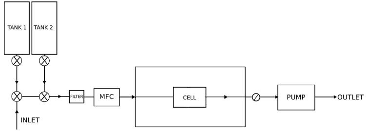
Figure 1Schematic of FCHAOS, in which air flows from the inlet line through the solenoid valves, past the filter to the mass flow controller (MFC), through the instrument cell, a needle valve, and finally the vacuum pump. When calibrating, the solenoid valves are actuated to direct flow from each individual calibration tank into the cell directly.
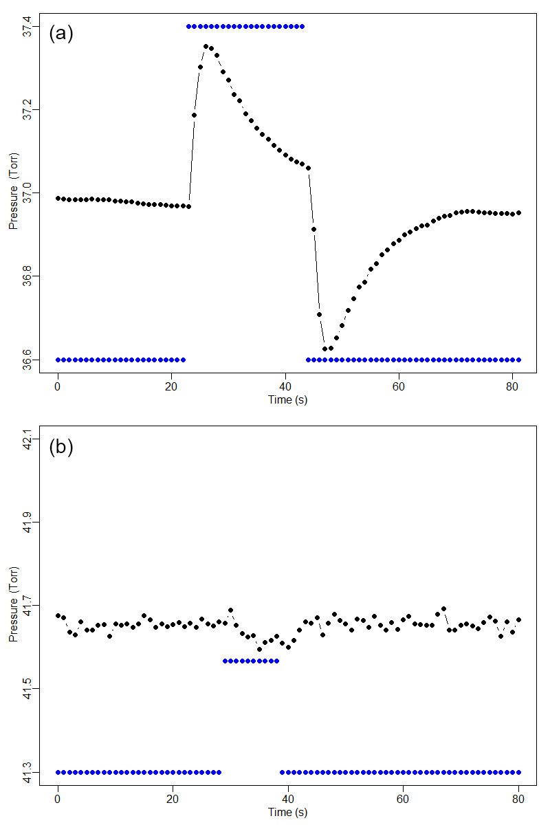
Figure 2Cell pressure (black) in response to actuating a solenoid and sampling a standard cylinder (blue indicates solenoid position). The pressure control setup (a), including excess flow, exhibits significant pressure perturbations and residual transients that persist longer than the desired calibration time. The mass flow control setup (b) shows pressure perturbations of shorter duration and on the order of 0.04 Torr, 20 times smaller than with pressure control.
2.3 Calibration
We performed pre-flight calibrations on the ground for both the FCHAOS and Picarro G2301-f using two air cylinders calibrated to a NOAA World Meteorological Organization (WMO) greenhouse gas scale (X2007, X2004A, X2014A, and X2006A for CO2, CH4, CO, and N2O, respectively) (WMO, 2015). Both cylinders had mixing ratios of CO2 (Tans et al., 2017; Zhao and Tans, 2006; Zhao et al., 1997), CH4 (Dlugokencky et al., 2005), CO (Novelli et al., 2003), and N2O (Hall et al., 2007) near ambient atmospheric levels, with one as a high-span standard and the other as a low-span.
We sequentially sampled these cylinders for multiple cycles, and compared the measured mixing ratios for each gas to the reported value on the WMO scale. We consider known values Xtrue against the measured values Xmeasured, and a linear fit provides the slope m and intercept b such that .
We filled the two in-flight calibration tanks used with the FCHAOS for FEAST with a separate custom mixture that contained atmospheric levels of N2O, CO2, and CO. We calibrated the mixing ratios using the WMO standard cylinders by sampling the target cylinders in between the WMO standards. During flights, we used one tank as a single-point calibration gas, while the other was used as a “check gas” to assess the instrument's traceability. We elaborate on these processes in Sects. 3.2 and 4.1.
We assessed the stability in slope of the instrument by performing calibrations separated by months before and after the FEAST campaign. Over the course of 4 months, the slopes for N2O, CO2, and CO changed by 0.4 %, 0.01 %, and 0.5 %. The impact of any variation in slope depends on the difference between ambient levels and calibration gas values. For the operation of FCHAOS, we use calibration gas with mixing ratios near ambient levels. Typical atmospheric ambient levels of N2O are ∼335 ppb, so with a calibration gas at ∼330 ppb, the long-term variation due to linearity is 0.4 % of 5 ppb, or 0.02 ppb, an uncertainty that is within our 1 Hz precision as reported in Sect. 4.1. For CO2 and CO, which have ambient atmospheric levels of ∼400 ppm and ∼155 ppb, we use calibration gases with ∼390 ppm and ∼150 ppb, and the impacts due to variation in slope are 0.01 ppm and 0.025 ppb, respectively. If zero air were used instead, the impact on N2O would be on the order of 0.4 % of 335 ppb, or 1.3 ppb, an order of magnitude larger, with similar impacts for CO2 and CO. By using calibration gases close to ambient levels we eliminate our sensitivity to drift in the instrument's slope and thus can use a single gas target for in-flight calibration to correct only for intercept variability.
2.4 Water vapor corrections
Spectroscopic measurements of atmospheric species are sensitive to dilution and broadening effects due to water vapor (Chen et al., 2010, 2013; Rella et al., 2013). TDLWintel, in its retrieval algorithm, corrects for water dilution and uses H2O broadening coefficients to mitigate the effect of water vapor on the spectral lines, directly reporting dry molar fractions for N2O, CO2, and CO (Lebegue et al., 2016; Pitt et al., 2016). This coefficient is the ratio of spectral line broadening due to water pressure compared to air pressure broadening. To determine the coefficients, we conducted a test in which dry tank air was sampled with varying amounts of water vapor. We used a similar approach as in Lebegue et al. (2016). We used a moist filter along with variable flow through parallel dry tubing, enabling some control of the water vapor content by modulating the relative flows over the moist filter compared to the dry tubing. We sampled at varying humidity starting at ∼1.6 % H2O and decreasing to near 0, spanning a typical range of atmospheric water vapor. Using spectral playback in TDLWintel, we were able to reanalyze the spectra with various broadening coefficients until we found the optimum values as in Pitt et al. (2016). Figure 3 shows the measurement data from the test using our optimized broadening coefficients of 1.33, 1.93, and 1 for N2O, CO2, and CO, respectively. The dry value is determined from prolonged sampling of dry air only from the standard tank. The deviation from this is shown as a function of water vapor. The gray line shows a moving average with a 10 s window. The root mean square difference in N2O, CO2, and CO was 0.023 ppb, 0.076 ppm, and 0.75 ppb, respectively. These are used as the uncertainty in water vapor correction, as in Pitt et al. (2016). For CO, a coefficient of 1 corresponds to purely a dilution correction. Larger values of the coefficient do not improve the dependency. As highlighted by Pitt et al. (2016), water broadening coefficients must be determined by users for their own instrument as these can vary for each analyzer and can introduce substantial errors in correcting to dry air mole fraction.
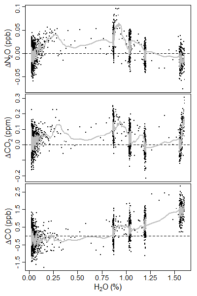
Figure 3Residual uncertainty in water vapor correction for N2O, CO2, and CO with broadening coefficients of 1.33, 1.93, and 1, respectively. Black dots are the deviation from the dry value, with a moving average (10 s) depicted in gray.
3.1 Null test
For an instrument to be well suited for airborne observation, resistance to environmental effects is paramount. A “null test”, in which an instrument samples air with known mixing ratios in flight while subject to variation in cabin pressure, air temperature, etc., can be useful in evaluating its robustness as shown in Chen et al. (2010) and Karion et al. (2013). We conducted two null tests using the FCHAOS, once during a test flight in Colorado, once during a research flight in our target region in the lower Mississippi River basin. Figure 4 shows N2O, CO2, and CO mixing ratios observed by the FCHAOS while sampling tank air during a vertical profile descent. As the altitude decreases, there is a clear dependence due to the cabin pressure changing similar to what was reported in Pitt et al. (2016). As mentioned in Sect. 2, though the cell is pressurized, the rest of the instrument is not, and since the aircraft cabin is not pressurized, our system thus experiences any change in ambient pressure. Correcting or mitigating this cabin pressure artifact is necessary for FCHAOS to be capable of accurate airborne in situ sampling.
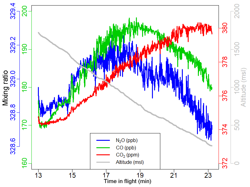
Figure 4A null test demonstrates artifacts when operating the instrument in an off-the-shelf manner. Drift occurs in N2O, CO2, and CO due to changes in cabin pressure that occur with changing aircraft altitude.
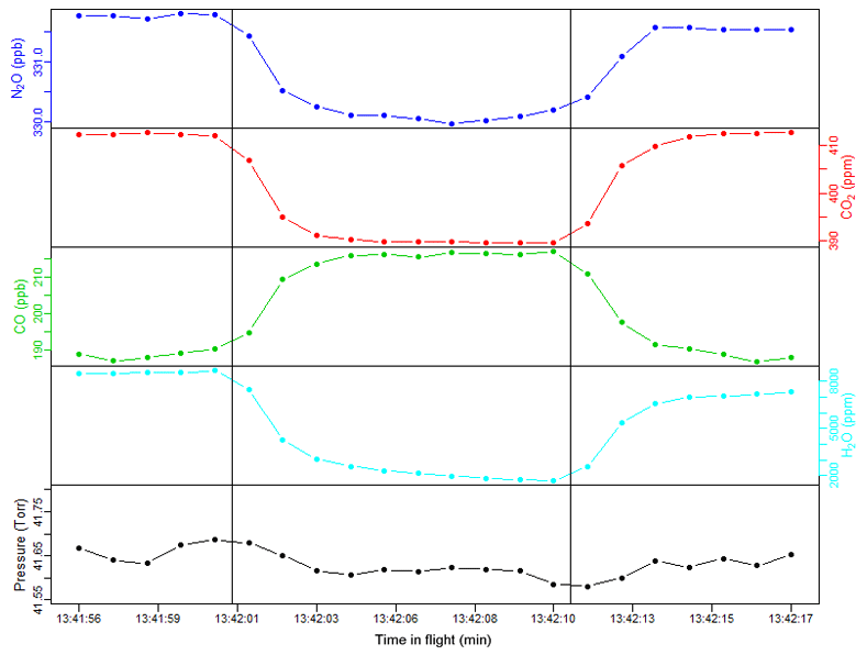
Figure 5Example of in-flight calibration, showing time series of N2O, CO2, CO, H2O, and cell pressure. Vertical lines indicate when the solenoid valve was actuated or closed. The first 5 s of each calibration is treated as equilibration time, and the last 5 s is used to find a mean calibration value.
3.2 Frequent calibration correction
The cause of the cabin pressure dependence is not immediately evident. One possible explanation could be an optical fringe pattern in the absorption spectrum that moves with changing cabin pressure. Acceleration during altitude change could also create G-force or electrical (via engine surges) changes that propagate through the instrument system. Without needing to pinpoint the cause, we know the time period of the artifact presents on the order of many minutes, with a typical aircraft climb rate of 500 ft min−1. Thus a correction that occurs on a shorter time spacing could remedy the drift. To account for both spectral drift in the instrument that occurs on the order of hours and cabin-pressure-related artifacts that emerge on the order of minutes, we developed an empirical correction procedure using frequent measurements of a calibration gas.
The procedure is as follows. Every 2 min, we actuate the solenoid valve to sample tank air for 10 s. We determined the calibration frequency of 2 min through a sensitivity test using null test data. By adjusting the calibration frequency and measuring the precision, we found similar 1σ uncertainties at 1 and 2 min frequencies, but an increase in uncertainty at 4 min and beyond, making 2 min good for reducing gas consumption while maintaining high precision. We allow 5 s of flush time, leaving 5 s of measurement time. We determined the flush time duration of 5 s by sampling tank air in a lab setting at the same flow rate and cell pressure as in-flight operation and measuring equilibration time. We calculate the average measured mole fraction of N2O, CO2, and CO in these 5 s. Figure 5 demonstrates a typical in-flight calibration.
For each species we then interpolated in time using a Forsythe, Malcom, and Moler cubic spline between each measured calibration gas value and subtracted the known “true” value from this interpolation, giving us the correction as a function of time. We then subtract this calibration curve from the raw data. Figure 6 shows both raw CO2 data and the correction we derive using the frequent calibration method from one of our flights. As mentioned above, the gas was on for 10 s, along with 5 s of post-calibration time removed to account for equilibration back to ambient sampling, resulting in a loss of 15 s of atmospheric observations every 120 s for an 87.5 % duty cycle. As mentioned in Sect. 2.3, the calibration cylinder mixing ratios are near atmospheric values. As seen in Santoni et al. (2014), N2O can take a long time to equilibrate between measurement sources due to its propensity to stick to tubing. Thus, choosing calibration values close to ambient levels is critical for maintaining short flush times. This also holds for CO2, though less so for CO. Artifacts that occur in shorter time frames, such as those induced by a short-duration turbulence event, will not be corrected with this method.
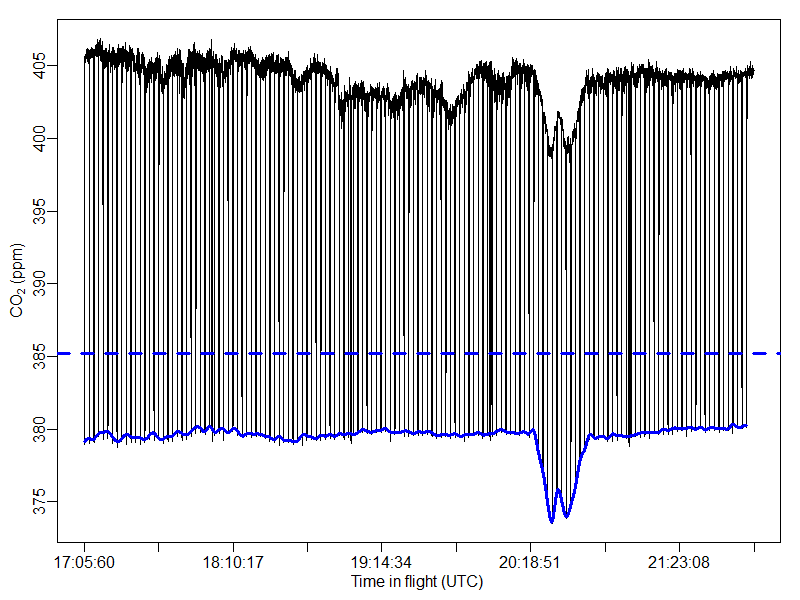
Figure 6Raw CO2 (black) measured by the FCHAOS for an entire flight, with frequent low dips due to calibrations. The blue dashed line indicates the “true” value of the calibration gas, and the blue solid line shows the calibration curve obtained by interpolating between each calibration instance. The difference between the dashed and solid blue lines is used to correct for drift.
Figure 7 shows measurements from two null tests, one on 26 April 2017 in Colorado and one on 2 May 2017 in the Mississippi River valley, the same null test as from Fig. 4. For each null test, the figure shows both the raw N2O, CO, and CO2 measurements and the corrected data following our calibration, along with the aircraft altitude. Our calibration method accounts for the clear cabin pressure–altitude dependence. During a null test FCHAOS samples tank air uninterrupted, rather than making a calibration measurement every 2 min as in the frequent calibration procedure described in Sect. 3.2. Thus, we average 5 s of data from every 120 s to simulate the normal operation mode. Even after correction there is some residual coherent variability evident at the 15 min mark of the null test shown in Fig. 7b, but this potential feature remains still within our 1 Hz precision.
Given the repeatable, smooth nature of the cabin pressure artifact, it would seem possible to use just the cabin pressure data to empirically correct for the artifact, without running frequent calibrations. This method would not account for long-term spectral drift, however, or traceability, and relies on the assumption that the cabin pressure artifact will be stable and repeatable. These weaknesses compromise such an approach.
Figure 8 compares the raw CO2 data from the Picarro G2301-f and FCHAOS during a research flight along with altitude, and a second comparison once the FCHAOS data are corrected. The difference between the two instruments is shown in panel a. The most significant discrepancies occur during the vertical profile section of the flight. Following calibration, the deviation during profiling is eliminated, and the 1σ uncertainty in the difference is reduced from 1.15 to 0.28 ppm.
For the FEAST campaign, in post-processing it became evident that a persistent offset of 0.51 ppm existed for CO2 between the Picarro and FCHAOS. For the CO2 comparisons in this paper, we have corrected for this bias. We believe the origin of this offset to be related to regulator contamination of a calibration gas cylinder and/or tubing used in conjunction with the regulator. With subsequent investigation it has been difficult to identify the exact cause. We do note that in comparing the Picarro and FCHAOS instruments, they both are calibrated with dry tank air, whereas the in-flight comparison is while measuring wet ambient air. Any residual water vapor sensitivity not corrected for either analyzer can manifest as an apparent bias, and this further emphasizes the need to validate water vapor corrections, as pointed out by Pitt et al. (2016), and further outlined for FCHAOS above in the discussion of the water vapor correction.
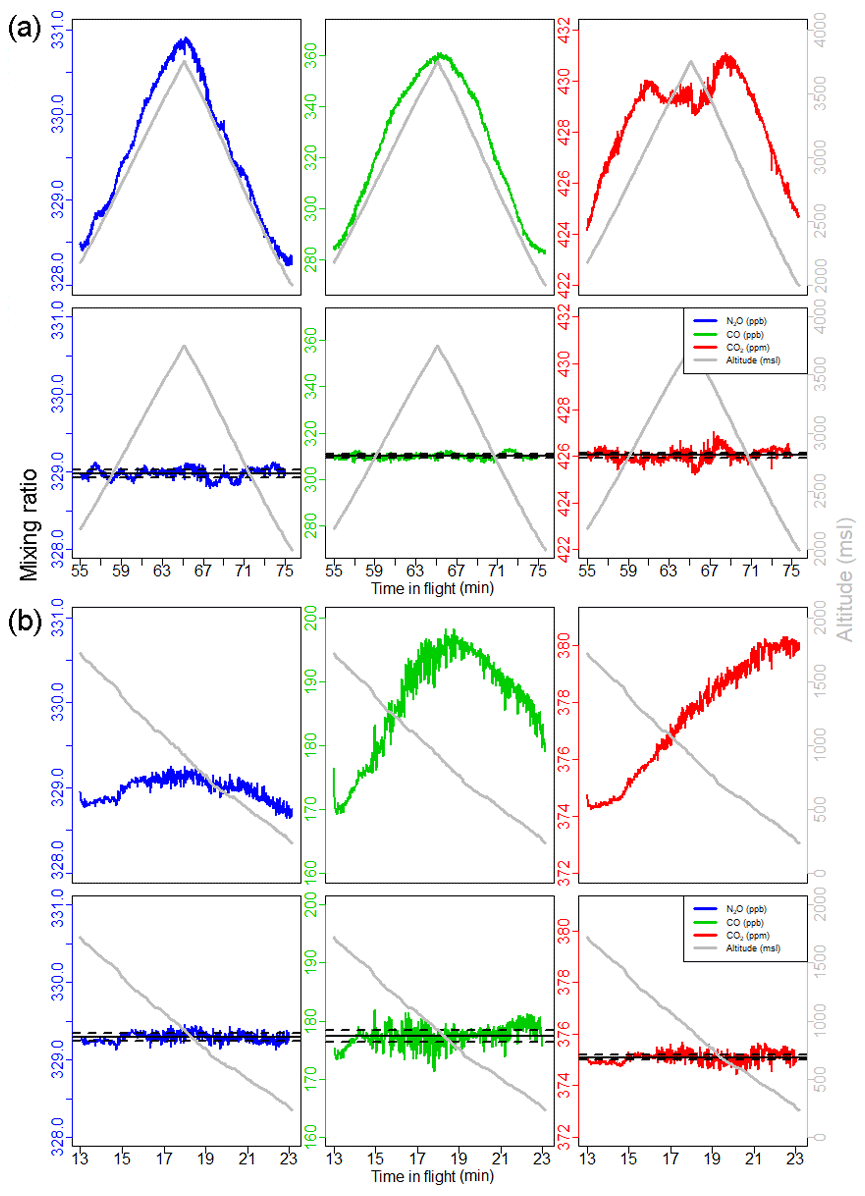
Figure 7Panel (a) shows FCHAOS data from a null test on 26 April 2017, and panel (b) shows data from a null test on 2 May 2017, the same seen in Fig. 4. Rows 1 and 3 show N2O, CO, and CO2 during the null test before any calibration, and rows 2 and 4 show the gas data following the frequent calibration correction. The procedure removes cabin pressure dependence and calibrates for linear drift. Black horizontal lines show mean and 1σ uncertainty.
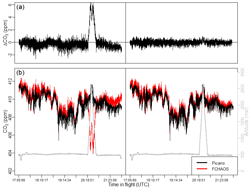
Figure 8Panel (b) shows Picarro G2301-f and uncalibrated FCHAOS CO2 time series on left, Picarro G2301-f and calibrated FCHAOS CO2 on right. Panel (a) shows the difference between the two instruments with and without FCHAOS calibration. The calibration procedure corrects for any artifacts in the FCHAOS data correlated with aircraft altitude.
The raw H2O measurements exhibit good agreement between FCHAOS and the Picarro G2301-f. The H2O data were not calibrated or adjusted in any way, as there appeared to be a small impact from cabin pressure variance and it is not well characterized. Figure 9 shows a histogram of the differences in FCHAOS and Picarro G2301-f H2O and CO2 (following calibration) for ∼40 h of research flight time. Figure 10 shows the differences as a function of time for all flight data. For H2O, we find a mean difference between the two instruments of 180 ppm, a median of 180 ppm, and 1σ of 340 ppm, shown in the figures as solid and dashed lines. In-flight 1σ precision for H2O from the Picarro G2301-f has been reported to be 100 ppm (Crosson, 2008), while the in-flight 1σ precision for the FCHAOS was found to be 10 ppm.
Why does water vapor not exhibit the same sensitivities as the other gases? To assess the sensitivity of water vapor to cabin pressure is more challenging given the long equilibration time. In Fig. 11 we show H2O during the null test. In the null test in which water vapor has previously equilibrated, some altitude-dependent sensitivity is apparent (∼60 ppm). Our calibration approach cannot address this potential residual sensitivity well given the long equilibration time required for H2O. Does this potential artifact matter? In comparison with the Picarro analyzer (Fig. 11) we see no evident residual sensitivity to altitude. Given relative uncertainties, we cannot eliminate the presence of a vertical sensitivity of 10s ppm for water vapor.
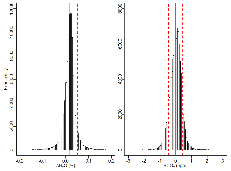
Figure 9Histogram of the difference between H2O and CO2 mixing ratios from FCHAOS and the Picarro G2301-f. FCHAOS CO2 has been calibrated, while H2O has not. For H2O, there is a mean of 0.018 % or 180 ppm, median of 0.018 % or 180 ppm, and 1σ of 0.034 % or 340 ppm, for which Picarro G2301-f precision is 100 ppm. For CO2, there is a mean of 0 ppm, median of 0.024 ppm, and 1σ of 0.45 ppm.

Figure 10Difference as a function of flight time for FCHAOS and Picarro G2301-f H2O and CO2 for all research flights. Colors separate flight days, and gray lines indicate mean and 1σ uncertainty. Largest deviations occur when sampling in the immediate near field of large point sources where some mismatched lag times contribute to deviations.

Figure 11Panels (a) and (b) show H2O during null tests from Fig. 7. In (b) H2O has not fully equilibrated. In (a), H2O previously equilibrated and there does appear to be a dependence on altitude on the order of 60 ppm. As seen in (c), the difference in H2O between the Picarro and FCHAOS over the entire campaign does not exhibit an altitude dependence, so while there may be some altitude sensitivity, the effect is relatively small compared to typical atmospheric concentrations of H2O and our overall water vapor uncertainty.
Precision and accuracy
To assess the FCHAOS precision, we consider flight data during a null test when the altitude did not significantly change. We find 1 s precisions of ±0.05 ppb, ±0.10 ppm, ±1.00 ppb, and ±10 ppm for N2O, CO2, CO, and H2O respectively. This is about a factor of 2 greater than the performance on the ground in a lab setting, with 1σ precisions of 0.02 ppb, 0.05 ppm, 0.50 ppb, and 7 ppm. Considering an Allan variance analysis of both the in-flight null test and in-lab study, the same result holds, in that the Allan variance in the air closely matches the ground, with performance degraded by a factor of 2.
In addition to the frequent calibrations every 2 min, a second cylinder is sampled every hour for 25 s as a check gas to test the traceability of the in-flight system. The last 5 s of each check gas period is used to calculate a mean value for each species. Figure 12 shows each instance of N2O, CO2, and CO check gas sampling, along with histograms for the difference from the known value. The time series show the last 5 s of each check gas period, along with a horizontal line indicating the known value of the air tank calibrated with the WMO standards as in Sect. 2.3. Note that the check gas and “calibration gas” cylinders were switched halfway through the campaign due to gas consumption, as reflected by the horizontal line. Looking at the difference of each check gas period from the known value, we find median offsets of 0.06 ppb, 0.06 ppm, and 0.03 ppb for N2O, CO2, and CO, respectively, representative of possible bias between the flight system and the WMO scale. The 1σ values for the check gas points are 0.10 ppb, 0.30 ppm, and 1.62 ppb for N2O, CO2, and CO, representative of traceability of individual 1 s observations to the WMO scale. Table 1 summarizes the precision and accuracy for the four gases, though we were unable to measure H2O traceability because we calibrated with dry tank air. We do report water vapor (and carbon dioxide) performance in comparison with the Picarro. Total instrument 1 s uncertainty is derived from summing in quadrature the 1σ accuracy to WMO, water vapor correction, and standard tank calibration uncertainty.
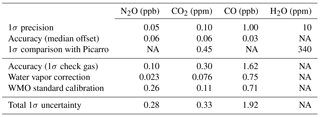
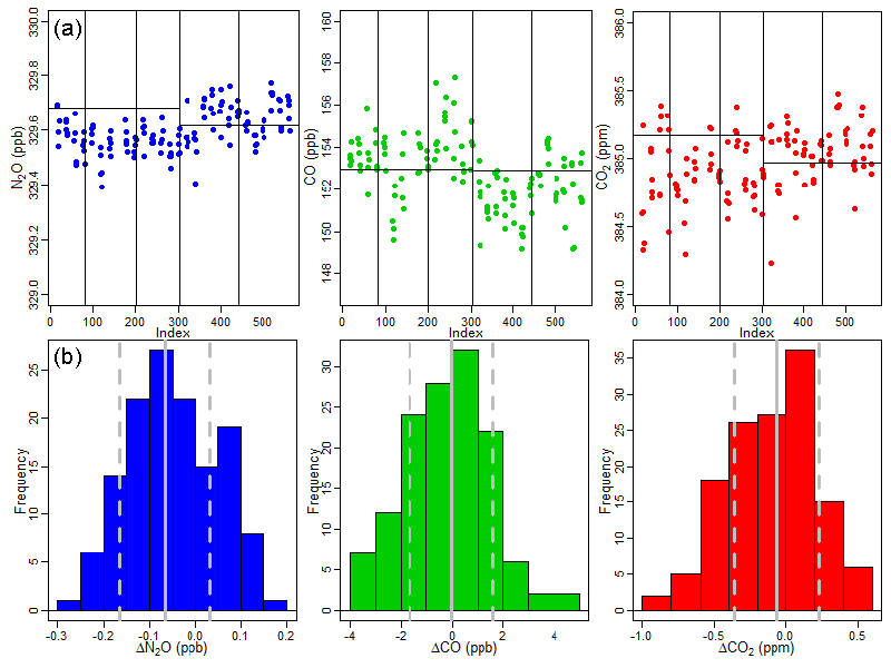
Figure 12(a) The last 5 s of each check gas period, the black horizontal line indicating the value of the sampled gas traced to the WMO scale. Vertical lines separate the individual research flights. (b) Histograms of the difference between the known check gas value and the last 5 s of measured check gas value, with solid gray lines indicating the median and dashed lines showing the 1σ uncertainty.
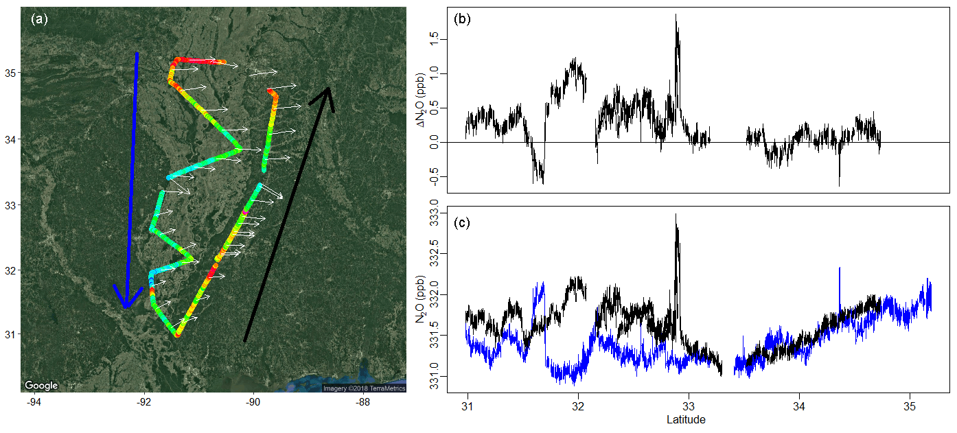
Figure 13(a) Flight path with N2O signal and wind direction (white arrows). Blue and black arrows show the direction of the plane's route and indicate upwind and downwind transects. (c) N2O signal as a function of latitude with upwind and downwind transects colored by blue and black, respectively. (b) Difference in N2O between downwind and upwind transects as a function of latitude.
Continuous airborne N2O observations can be useful for quantifying fluxes and estimating emissions on a facility–regional scale. Mass balances techniques, which have been utilized to estimate emissions of other atmospheric gases as in Karion et al. (2013), Smith et al. (2015), Peischl et al. (2015), and Kort et al. (2016), could similarly be applied for N2O. Figure 13 shows the path flown during a research flight on 6 May 2017, with measured N2O mole fraction in color, white arrows indicating wind direction and speed, and blue and black arrows showing the direction of the flight route and the upwind and downwind transects. The downwind transect was flown at a mean altitude of 1515 msl, 1σ of 14 m, and the upwind transect at a mean altitude of 1501 msl, 1σ of 14 m. Panel c of the figure shows N2O from this flight as a function of latitude with the upwind and downwind transects in blue and black, while panel b shows the difference in N2O between the downwind and upwind at each latitude. There is a distinct enhancement in the downwind transect relative to the upwind transect in the lower latitudes, from about 31.5 to 32∘ N. This enhancement disappears at higher latitudes and the N2O measurement tracks well between upwind and downwind transects, even with a substantial latitudinal gradient. This flight illustrates the ability of this instrument to accurately measure small variations and link to local emissions (to the south) or larger scale gradients (to the north). Future analyses of these data can involve mass balance flux quantification and/or regional model comparisons, both to quantify emissions and to link to driving factors such as soil moisture or crop type.
As a fast-response sensor, FCHAOS can also be used for point source quantifications, as first explained in Conley et al. (2017) and further analyzed in Mehrotra et al. (2017) and Vaughn et al. (2017). During FEAST, we circled several fertilizer plants with significant N2O emissions, and future analyses can leverage these observations to better quantify emissions from the large point sources.
We present a continuous-wave, mid-IR laser spectrometer system that can measure continuous 1 Hz airborne mole fractions of N2O, CO2, CO, and H2O. The commercial analyzer, when operated off the shelf, exhibits a dependence of N2O, CO2, and CO on cabin pressure. We correct for this artifact by employing an updated calibration procedure with mass flow control at a high flow rate enabling high-frequency, short-duration calibrations. While modern systems conventionally use pressure control and infrequent, long-duration zeros, our method expands on these previous approaches and opens up uses for the instrument in ways that have not yet been realized. We solve the inability of other systems to operate with large changes in cabin pressure by mitigating the cabin pressure effect while maintaining a ∼90 % duty cycle. In-flight 1σ precisions are estimated to be ±0.05 ppb, ±0.10 ppm, ±1.00 ppb, and ±10 ppm for N2O, CO2, CO, and H2O, with total uncertainty in traceability estimated at 0.28 ppb, 0.33 ppm, and 1.92 ppb for N2O, CO2, and CO. We then validate our method by comparing FCHAOS data to CO2 and H2O measurements from a flight-proven cavity ring-down spectrometer, seeing excellent agreement. This flight-proven system can provide key insights into N2O emissions processes by providing observational support for facility quantification, for mass balance flux estimates, and for inverse modeling. As presented, this system can be utilized for precise, accurate, continuous 1 Hz airborne observations of N2O, CO2, CO, and H2O.
The dataset presented in this paper is accessible at the University of Michigan Deep Blue Data Repository; see Kort et al. (2018).
All authors contributed to flight planning and logistics. EAK, AG, and MLS collected the data with contributions from SC. AG performed the analysis with contributions from all other authors. AG and EAK wrote the manuscript.
The authors declare that they have no conflict of interest.
We thank Scientific Aviation pilots for their efforts in helping collect
these data and Aerodyne Research Inc. for useful discussions. This material is
based partly upon work supported by the National Science Foundation under
grant no. 1650682.
Edited by: Marc von
Hobe
Reviewed by: Joseph Pitt and two anonymous referees
Bouwman, A. F., Boumans, L. J. M., and Batjes, N. H.: Emissions of N2O and NO from fertilized fields: Summary of available measurement data, Global Biogeochem. Cy., 16, 6-1–6-13, https://doi.org/10.1029/2001GB001811, https://doi.org/10.1029/2001GB001811, 2002. a
Brown, L., Armstrong Brown, S., Jarvis, S. C., Syed, B., Goulding, K. W. T., Phillips, V. R., Sneath, R. W., and Pain, B. F.: An inventory of nitrous oxide emissions from agriculture in the UK using the IPCC methodology: emission estimate, uncertainty and sensitivity analysis, Atmos. Environ., 35, 1439–1449, https://doi.org/10.1016/S1352-2310(00)00361-7, 2001. a
Chadwick, D. R., Cardenas, L., Misselbrook, T. H., Smith, K. A., Rees, R. M., Watson, C. J., McGeough, K. L., Williams, J. R., Cloy, J. M., Thorman, R. E., and Dhanoa, M. S.: Optimizing chamber methods for measuring nitrous oxide emissions from plot-based agricultural experiments, Eur. J. Soil Sci., 65, 295–307, 2014. a
Chen, H., Winderlich, J., Gerbig, C., Hoefer, A., Rella, C. W., Crosson, E. R., Van Pelt, A. D., Steinbach, J., Kolle, O., Beck, V., Daube, B. C., Gottlieb, E. W., Chow, V. Y., Santoni, G. W., and Wofsy, S. C.: High-accuracy continuous airborne measurements of greenhouse gases (CO2 and CH4) using the cavity ring-down spectroscopy (CRDS) technique, Atmos. Meas. Tech., 3, 375–386, https://doi.org/10.5194/amt-3-375-2010, 2010. a, b, c
Chen, H., Karion, A., Rella, C. W., Winderlich, J., Gerbig, C., Filges, A., Newberger, T., Sweeney, C., and Tans, P. P.: Accurate measurements of carbon monoxide in humid air using the cavity ring-down spectroscopy (CRDS) technique, Atmos. Meas. Tech., 6, 1031–1040, https://doi.org/10.5194/amt-6-1031-2013, 2013. a
Chen, Z., Griffis, T. J., Millet, D. B., Wood, J. D., Lee, X., Baker, J. M., Xiao, K., Turner, P. A., Chen, M., Zobitz, J., and Wells, K. C.: Partitioning N2O emissions within the U.S. Corn Belt using an inverse modeling approach, Global Biogeochem. Cy., 30, 1192–1205, https://doi.org/10.1002/2015GB005313, 2016. a
Ciais, P., Chris, S., Govindasamy, B., Bopp, L., Brovkin, V., Canadell, J., Chhabra, A., Defries, R., Galloway, J., and Heimann, M.: Carbon and other biogeochemical cycles, 465–570, Cambridge University Press, 2013. a
Conley, S., Faloona, I., Mehrotra, S., Suard, M., Lenschow, D. H., Sweeney, C., Herndon, S., Schwietzke, S., Pétron, G., Pifer, J., Kort, E. A., and Schnell, R.: Application of Gauss's theorem to quantify localized surface emissions from airborne measurements of wind and trace gases, Atmos. Meas. Tech., 10, 3345–3358, https://doi.org/10.5194/amt-10-3345-2017, 2017. a, b, c
Conley, S. A., Faloona, I. C., Lenschow, D. H., Karion, A., and Sweeney, C.: A Low-Cost System for Measuring Horizontal Winds from Single-Engine Aircraft, J. Atmos. Ocean. Tech., 31, 1312–1320, https://doi.org/10.1175/JTECH-D-13-00143.1, 2014. a, b
Crosson, E.: A cavity ring-down analyzer for measuring atmospheric levels of methane, carbon dioxide, and water vapor, Appl. Phys. B-Lasers O., 92, 403–408, https://doi.org/10.1007/s00340-008-3135-y, 2008. a, b
Dalal, R. C., Wang, W., Robertson, G. P., and Parton, W. J.: Nitrous oxide emission from Australian agricultural lands and mitigation options: a review, Aust. J. Soil Res., 41, 165, https://doi.org/10.1071/sr02064, 2003. a, b
Davidson, E. A. and Kanter, D.: Inventories and scenarios of nitrous oxide emissions, Environ. Res. Lett., 9, 105012, http://stacks.iop.org/1748-9326/9/i=10/a=105012, 2014. a, b
Del Grosso, S. J., Parton, W. J., Mosier, A. R., Walsh, M. K., Ojima, D. S., and Thornton, P. E.: DAYCENT National-Scale Simulations of Nitrous Oxide Emissions from Cropped Soils in the United States, J. Environ. Qual., 35, 1451–1460, 2006. a
Denmead, O.: Approaches to measuring fluxes of methane and nitrous oxide between landscapes and the atmosphere, Plant Soil, 309, 1–2, 5, 2008. a
Dlugokencky, E. J., Myers, R. C., Lang, P. M., Masarie, K. A., Crotwell, A. M., Thoning, K. W., Hall, B. D., Elkins, J. W., and Steele, L. P.: Conversion of NOAA atmospheric dry air CH4 mole fractions to a gravimetrically prepared standard scale, J. Geophys. Res.-Atmos., 110, D18306, https://doi.org/10.1029/2005JD006035, 2005. a
Erisman, J., Sutton, M., Galloway, J., Klimont, Z., and Winiwarter, W.: How a century of ammonia synthesis changed the world, Nat. Geosci., 1, 636–639, https://doi.org/10.1038/ngeo325, 2008. a
Filges, A., Gerbig, C., Chen, H., Franke, H., Klaus, C., and Jordan, A.: The IAGOS-core greenhouse gas package: a measurement system for continuous airborne observations of CO2, CH4, H2O and CO, Tellus B, 67, 27989, https://doi.org/10.3402/tellusb.v67.27989, 2015. a
Flechard, C., Ambus, P., Skiba, U., Rees, R., Hensen, A., van Amstel, A., van den Pol-van Dasselaar, A., Soussana, J.-F., Jones, M., Clifton-Brown, J., Raschi, A., Horvath, L., Neftel, A., Jocher, M., Ammann, C., Leifeld, J., Fuhrer, J., Calanca, P., Thalman, E., Pilegaard, K., Marco, C. D., Campbell, C., Nemitz, E., Hargreaves, K., Levy, P., Ball, B., Jones, S., van de Bulk, W., Groot, T., Blom, M., Domingues, R., Kasper, G., Allard, V., Ceschia, E., Cellier, P., Laville, P., Henault, C., Bizouard, F., Abdalla, M., Williams, M., Baronti, S., Berretti, F., and Grosz, B.: Effects of climate and management intensity on nitrous oxide emissions in grassland systems across Europe, Agr. Ecosyst. Environ., 121, 135–152, https://doi.org/10.1016/j.agee.2006.12.024, the Greenhouse Gas Balance of Grasslands in Europe, 2007. a
Frankenberg, C., Kulawik, S. S., Wofsy, S. C., Chevallier, F., Daube, B., Kort, E. A., O'Dell, C., Olsen, E. T., and Osterman, G.: Using airborne HIAPER Pole-to-Pole Observations (HIPPO) to evaluate model and remote sensing estimates of atmospheric carbon dioxide, Atmos. Chem. Phys., 16, 7867–7878, https://doi.org/10.5194/acp-16-7867-2016, 2016. a
Fried, A., Diskin, G., Weibring, P., Richter, D., Walega, J., Sachse, G., Slate, T., Rana, M., and Podolske, J.: Tunable infrared laser instruments for airborne atmospheric studies, Appl. Phys. B-Lasers O., 92, 409–417, https://doi.org/10.1007/s00340-008-3136-x, 2008. a
Griffis, T. J., Chen, Z., Baker, J. M., Wood, J. D., Millet, D. B., Lee, X., Venterea, R. T., and Turner, P. A.: Nitrous oxide emissions are enhanced in a warmer and wetter world, P. Natl. Acad. Sci., 114, 12081–12085, https://doi.org/10.1073/pnas.1704552114, 2017. a, b
Hall, B. D., Dutton, G. S., and Elkins, J. W.: The NOAA nitrous oxide standard scale for atmospheric observations, J. Geophys. Res.-Atmos., 112, D09305, https://doi.org/10.1029/2006JD007954, 2007. a
Inoue, M., Morino, I., Uchino, O., Nakatsuru, T., Yoshida, Y., Yokota, T., Wunch, D., Wennberg, P. O., Roehl, C. M., Griffith, D. W. T., Velazco, V. A., Deutscher, N. M., Warneke, T., Notholt, J., Robinson, J., Sherlock, V., Hase, F., Blumenstock, T., Rettinger, M., Sussmann, R., Kyrö, E., Kivi, R., Shiomi, K., Kawakami, S., De Mazière, M., Arnold, S. G., Feist, D. G., Barrow, E. A., Barney, J., Dubey, M., Schneider, M., Iraci, L. T., Podolske, J. R., Hillyard, P. W., Machida, T., Sawa, Y., Tsuboi, K., Matsueda, H., Sweeney, C., Tans, P. P., Andrews, A. E., Biraud, S. C., Fukuyama, Y., Pittman, J. V., Kort, E. A., and Tanaka, T.: Bias corrections of GOSAT SWIR XCO2 and XCH4 with TCCON data and their evaluation using aircraft measurement data, Atmos. Meas. Tech., 9, 3491–3512, https://doi.org/10.5194/amt-9-3491-2016, 2016. a
Karion, A., Sweeney, C., Wolter, S., Newberger, T., Chen, H., Andrews, A., Kofler, J., Neff, D., and Tans, P.: Long-term greenhouse gas measurements from aircraft, Atmos. Meas. Tech., 6, 511–526, https://doi.org/10.5194/amt-6-511-2013, 2013. a, b, c
Karion, A., Sweeney, C., Kort, E. A., Shepson, P. B., Brewer, A., Cambaliza, M., Conley, S. A., Davis, K., Deng, A., Hardesty, M., Herndon, S. C., Lauvaux, T., Lavoie, T., Lyon, D., Newberger, T., Pétron, G., Rella, C., Smith, M., Wolter, S., Yacovitch, T. I., and Tans, P.: Aircraft-Based Estimate of Total Methane Emissions from the Barnett Shale Region, Environ. Sci. Technol., 49, 8124–8131, https://doi.org/10.1021/acs.est.5b00217, 2015. a, b
Kort, E. A., Eluszkiewicz, J., Stephens, B. B., Miller, J. B., Gerbig, C., Nehrkorn, T., Daube, B. C., Kaplan, J. O., Houweling, S., and Wofsy, S. C.: Emissions of CH4 and N2O over the United States and Canada based on a receptor-oriented modeling framework and COBRA-NA atmospheric observations, Geophys. Res. Lett., 35, L18808, https://doi.org/10.1029/2008GL034031, 2008. a
Kort, E. A., Patra, P. K., Ishijima, K., Daube, B. C., Jiménez, R., Elkin, J., Hurst, D., Moore, F. L., Sweeney, C., and Wofsy, S. C.: Tropospheric distribution and variability of N2O: Evidence for strong tropical emissions, Geophys. Res. Lett., 38, L15806, https://doi.org/10.1029/2011GL047612, 2011. a, b
Kort, E. A., Smith, M. L., Murray, L. T., Gvakharia, A., Brandt, A. R., Peischl, J., Ryerson, T. B., Sweeney, C., and Travis, K.: Fugitive emissions from the Bakken shale illustrate role of shale production in global ethane shift, Geophys. Res. Lett., 43, 4617–4623, https://doi.org/10.1002/2016GL068703, 2016. a, b, c
Kort, E. A., Gvakharia, A., Smith, M. L., and Conley, S.: Airborne Data from the Fertilizer Emissions Airborne Study (FEAST). Nitrous Oxide, Carbon Dioxide, Carbon Monoxide, Methane, Ozone, Water Vapor, and meteorological variables over the Mississippi River Valley [Data set], University of Michigan Deep Blue Data Repository, https://doi.org/10.7302/Z2XK8CRG, 2018. a
Lebegue, B., Schmidt, M., Ramonet, M., Wastine, B., Yver Kwok, C., Laurent, O., Belviso, S., Guemri, A., Philippon, C., Smith, J., and Conil, S.: Comparison of nitrous oxide (N2O) analyzers for high-precision measurements of atmospheric mole fractions, Atmos. Meas. Tech., 9, 1221–1238, https://doi.org/10.5194/amt-9-1221-2016, 2016. a, b
Marinho, E. V. A., DeLaune, R. D., and Lindau, C. W.: Nitrous Oxide Flux from Soybeans Grown on Mississippi Alluvial Soil, Commun. Soil Sci. Plan., 35, 1–8, https://doi.org/10.1081/CSS-120027630, 2004. a
McManus, J. B., Kebabian, P. L., and Zahniser, M. S.: Astigmatic mirror multipass absorption cells for long-path-length spectroscopy, Appl. Opt., 34, 3336–3348, https://doi.org/10.1364/AO.34.003336, 1995. a
Mehrotra, S., Faloona, I., Suard, M., Conley, S., and Fischer, M. L.: Airborne Methane Emission Measurements for Selected Oil and Gas Facilities Across California, Environ. Sci. Technol., 51, 12981–12987, 2017. a, b
Miller, S. M., Kort, E. A., Hirsch, A. I., Dlugokencky, E. J., Andrews, A. E., Xu, X., Tian, H., Nehrkorn, T., Eluszkiewicz, J., Michalak, A. M., and Wofsy, S. C.: Regional sources of nitrous oxide over the United States: Seasonal variation and spatial distribution, J. Geophys. Res.-Atmos., 117, D06310, https://doi.org/10.1029/2011JD016951, 2012. a, b
Monni, S., Perälä, P., and Regina, K.: Uncertainty in Agricultural CH4 AND N2O Emissions from Finland – Possibilities to Increase Accuracy in Emission Estimates, Mitig. Adapt. Strat. Gl., 12, 545–571, https://doi.org/10.1007/s11027-006-4584-4, 2007. a
Myhre, G., Shindell, D., Bréon, F.-M., Collins, W., Fuglestvedt, J., Huang, J., Koch, D., Lamarque, J.-F., Lee, D., Mendoza, B., Nakajima, T., Robock, A., Stephens, G., Takemura, T., and Zhang, H.: Anthropogenic and natural radiative forcing, in: Climate Change 2013: The Physical Science Basis. Contribution of Working Group I to the Fifth Assessment Report of the Intergovernmental Panel on Climate Change, edited by: Stocker, T. F., Qin, D., Plattner, G.-K., Tignor, M., Allen, S. K., Doschung, J., Nauels, A., Xia, Y., Bex, V., and Midgley, P. M., 659–740, Cambridge University Press, Cambridge, UK, https://doi.org/10.1017/CBO9781107415324.018, 2013. a
Nelson, D., Shorter, J., McManus, J., and Zahniser, M.: Sub-part-per-billion detection of nitric oxide in air using a thermoelectrically cooled mid-infrared quantum cascade laser spectrometer, Appl. Phys. B-Lasers O., 75, 343–350, https://doi.org/10.1007/s00340-002-0979-4, 2002. a, b
Nelson, D. D., McManus, B., Urbanski, S., Herndon, S., and Zahniser, M. S.: High precision measurements of atmospheric nitrous oxide and methane using thermoelectrically cooled mid-infrared quantum cascade lasers and detectors, Spectrochim. Acta A, 60, 3325–3335, https://doi.org/10.1016/j.saa.2004.01.033, 2004. a, b
Nevison, C., Andrews, A., Thoning, K., Dlugokencky, E., Sweeney, C., Miller, S., Saikawa, E., Benmergui, J., Fischer, M., Mountain, M., and Nehrkorn, T.: Nitrous Oxide Emissions Estimated With the CarbonTracker-Lagrange North American Regional Inversion Framework, Global Biogeochem. Cy., 32, 463–485, https://doi.org/10.1002/2017GB005759, 2018. a
Novelli, P. C., Masarie, K. A., Lang, P. M., Hall, B. D., Myers, R. C., and Elkins, J. W.: Reanalysis of tropospheric CO trends: Effects of the 1997–1998 wildfires, J. Geophys. Res.-Atmos., 108, 4464, https://doi.org/10.1029/2002JD003031, 2003. a
O'Shea, S. J., Bauguitte, S. J.-B., Gallagher, M. W., Lowry, D., and Percival, C. J.: Development of a cavity-enhanced absorption spectrometer for airborne measurements of CH4 and CO2, Atmos. Meas. Tech., 6, 1095–1109, https://doi.org/10.5194/amt-6-1095-2013, 2013. a
O'Shea, S. J., Allen, G., Gallagher, M. W., Bower, K., Illingworth, S. M., Muller, J. B. A., Jones, B. T., Percival, C. J., Bauguitte, S. J.-B., Cain, M., Warwick, N., Quiquet, A., Skiba, U., Drewer, J., Dinsmore, K., Nisbet, E. G., Lowry, D., Fisher, R. E., France, J. L., Aurela, M., Lohila, A., Hayman, G., George, C., Clark, D. B., Manning, A. J., Friend, A. D., and Pyle, J.: Methane and carbon dioxide fluxes and their regional scalability for the European Arctic wetlands during the MAMM project in summer 2012, Atmos. Chem. Phys., 14, 13159–13174, https://doi.org/10.5194/acp-14-13159-2014, 2014. a
Pattey, E., Edwards, G., Desjardins, R., Pennock, D., Smith, W., Grant, B., and MacPherson, J.: Tools for quantifying N2O emissions from agroecosystems, Agr. Forest Meteorol., 142, 103–119, https://doi.org/10.1016/j.agrformet.2006.05.013, the Contribution of Agriculture to the State of Climate, 2007. a
Peischl, J., Ryerson, T. B., Aikin, K. C., Gouw, J. A., Gilman, J. B., Holloway, J. S., Lerner, B. M., Nadkarni, R., Neuman, J. A., Nowak, J. B., Trainer, M., Warneke, C., and Parrish, D. D.: Quantifying atmospheric methane emissions from the Haynesville, Fayetteville, and northeastern Marcellus shale gas production regions, J. Geophys. Res-Atmos., 120, 2119–2139, https://doi.org/10.1002/2014JD022697, 2015. a, b, c
Pennock, D., Farrell, R., Desjardins, R., Pattey, E., and MacPherson, J. I.: Upscaling chamber-based measurements of N2O emissions at snowmelt, Can. J. Soil Sci., 85, 113–125, https://doi.org/10.4141/S04-040, 2005. a
Pitt, J. R., Le Breton, M., Allen, G., Percival, C. J., Gallagher, M. W., Bauguitte, S. J.-B., O'Shea, S. J., Muller, J. B. A., Zahniser, M. S., Pyle, J., and Palmer, P. I.: The development and evaluation of airborne in situ N2O and CH4 sampling using a quantum cascade laser absorption spectrometer (QCLAS), Atmos. Meas. Tech., 9, 63–77, https://doi.org/10.5194/amt-9-63-2016, 2016. a, b, c, d, e, f, g, h, i
Rannik, Ü., Haapanala, S., Shurpali, N. J., Mammarella, I., Lind, S., Hyvönen, N., Peltola, O., Zahniser, M., Martikainen, P. J., and Vesala, T.: Intercomparison of fast response commercial gas analysers for nitrous oxide flux measurements under field conditions, Biogeosciences, 12, 415–432, https://doi.org/10.5194/bg-12-415-2015, 2015. a
Rapson, T. D. and Dacres, H.: Analytical techniques for measuring nitrous oxide, TrAC-Trend. Anal. Chem., 54, 65–74, https://doi.org/10.1016/j.trac.2013.11.004, 2014. a
Ravishankara, A. R., Daniel, J. S., and Portmann, R. W.: Nitrous Oxide (N2O): The Dominant Ozone-Depleting Substance Emitted in the 21st Century, Science, 326, 123–125, https://doi.org/10.1126/science.1176985, 2009. a
Rella, C. W., Chen, H., Andrews, A. E., Filges, A., Gerbig, C., Hatakka, J., Karion, A., Miles, N. L., Richardson, S. J., Steinbacher, M., Sweeney, C., Wastine, B., and Zellweger, C.: High accuracy measurements of dry mole fractions of carbon dioxide and methane in humid air, Atmos. Meas. Tech., 6, 837–860, https://doi.org/10.5194/amt-6-837-2013, 2013. a
Rothman, L. S., Gordon, I. E., Babikov, Y., Barbe, A., Chris Benner, D., Bernath, P. F., Birk, M., Bizzocchi, L., Boudon, V., Brown, L. R., Campargue, A., Chance, K., Cohen, E. A., Coudert, L. H., Devi, V. M., Drouin, B. J., Fayt, A., Flaud, J.-M., Gamache, R. R., Harrison, J. J., Hartmann, J.-M., Hill, C., Hodges, J. T., Jacquemart, D., Jolly, A., Lamouroux, J., Le Roy, R. J., Li, G., Long, D. A., Lyulin, O. M., Mackie, C. J., Massie, S. T., Mikhailenko, S., Müller, H. S. P., Naumenko, O. V., Nikitin, A. V., Orphal, J., Perevalov, V., Perrin, A., Polovtseva, E. R., Richard, C., Smith, M. A. H., Starikova, E., Sung, K., Tashkun, S., Tennyson, J., Toon, G. C., Tyuterev, V. G., and Wagner, G.: The HITRAN2012 molecular spectroscopic database, J. Quant. Spectrosc. Ra., 130, 4–50, https://doi.org/10.1016/j.jqsrt.2013.07.002, 2013. a
Ruser, R., Flessa, H., Russow, R., Schmidt, G., Buegger, F., and Munch, J.: Emission of N2O, N2 and CO2 from soil fertilized with nitrate: effect of compaction, soil moisture and rewetting, Soil Biol. Biochem., 38, 263–274, https://doi.org/10.1016/j.soilbio.2005.05.005, 2006. a
Santoni, G. W., Daube, B. C., Kort, E. A., Jiménez, R., Park, S., Pittman, J. V., Gottlieb, E., Xiang, B., Zahniser, M. S., Nelson, D. D., McManus, J. B., Peischl, J., Ryerson, T. B., Holloway, J. S., Andrews, A. E., Sweeney, C., Hall, B., Hintsa, E. J., Moore, F. L., Elkins, J. W., Hurst, D. F., Stephens, B. B., Bent, J., and Wofsy, S. C.: Evaluation of the airborne quantum cascade laser spectrometer (QCLS) measurements of the carbon and greenhouse gas suite – CO2, CH4, N2O, and CO – during the CalNex and HIPPO campaigns, Atmos. Meas. Tech., 7, 1509–1526, https://doi.org/10.5194/amt-7-1509-2014, 2014. a, b, c, d
Smith, M. L., Kort, E. A., Karion, A., Sweeney, C., Herndon, S. C., and Yacovitch, T. I.: Airborne Ethane Observations in the Barnett Shale: Quantification of Ethane Flux and Attribution of Methane Emissions, Environ. Sci. Technol., 49, 8158–8166, https://doi.org/10.1021/acs.est.5b00219, 2015. a, b, c, d
Tanaka, T., Yates, E., Iraci, L. T., Johnson, M. S., Gore, W., Tadić, J. M., Loewenstein, M., Kuze, A., Frankenberg, C., Butz, A., and Yoshida, Y.: Two-Year Comparison of Airborne Measurements of CO2 and CH4 With GOSAT at Railroad Valley, Nevada, IEEE T. Geosci. Remote, 54, 4367–4375, 2016. a
Tans, P. P., Crotwell, A. M., and Thoning, K. W.: Abundances of isotopologues and calibration of CO2 greenhouse gas measurements, Atmos. Meas. Tech., 10, 2669–2685, https://doi.org/10.5194/amt-10-2669-2017, 2017. a
Thompson, R. L., Chevallier, F., Crotwell, A. M., Dutton, G., Langenfelds, R. L., Prinn, R. G., Weiss, R. F., Tohjima, Y., Nakazawa, T., Krummel, P. B., Steele, L. P., Fraser, P., O'Doherty, S., Ishijima, K., and Aoki, S.: Nitrous oxide emissions 1999 to 2009 from a global atmospheric inversion, Atmos. Chem. Phys., 14, 1801–1817, https://doi.org/10.5194/acp-14-1801-2014, 2014. a
Tian, H., Chen, G., Lu, C., Xu, X., Ren, W., Zhang, B., Banger, K., Tao, B., Pan, S., Liu, M., Zhang, C., Bruhwiler, L., and Wofsy, S.: Global methane and nitrous oxide emissions from terrestrial ecosystems due to multiple environmental changes, Ecosystem Health and Sustainability, 1, 1–20, https://doi.org/10.1890/EHS14-0015.1, 2015. a
Turner, D. A., Chen, D., Galbally, I. E., Leuning, R., Edis, R. B., Li, Y., Kelly, K., and Phillips, F.: Spatial variability of nitrous oxide emissions from an Australian irrigated dairy pasture, Plant Soil, 309, 77–88, https://doi.org/10.1007/s11104-008-9639-8, 2008. a
Vaughn, T. L., Bell, C. S., Yacovitch, T. I., Roscioli, J. R., Herndon, S. C., Conley, S., Schwietzke, S., Heath, G. A., Pétron, G., and Zimmerle, D.: Comparing facility-level methane emission rate estimates at natural gas gathering and boosting stations, Elem. Sci. Anth., 5, 71, https://doi.org/10.1525/elementa.257, 2017. a
WMO, W.: 18th WMO/IAEA Meeting on Carbon Dioxide, Other Greenhouse Gases and Related Tracers Measurement Techniques (GGMT-2015), GAW Report-No. 229, 2015. a
Wofsy, S. C.: HIAPER Pole-to-Pole Observations (HIPPO): fine-grained, global-scale measurements of climatically important atmospheric gases and aerosols, Philos. T. Roy. Soc. A, 369, 2073–2086, https://doi.org/10.1098/rsta.2010.0313, 2011. a, b
Xiang, B., Miller, S. M., Kort, E. A., Santoni, G. W., Daube, B. C., Commane, R., Angevine, W. M., Ryerson, T. B., Trainer, M. K., Andrews, A. E., Nehrkorn, T., Tian, H., and Wofsy, S. C.: Nitrous oxide (N2O) emissions from California based on 2010 CalNex airborne measurements, J. Geophys. Res.-Atmos., 118, 2809–2820, https://doi.org/10.1002/jgrd.50189, 2013. a
Yacovitch, T. I., Herndon, S. C., Roscioli, J. R., Floerchinger, C., McGovern, R. M., Agnese, M., Pétron, G., Kofler, J., Sweeney, C., Karion, A., Conley, S. A., Kort, E. A., Nähle, L., Fischer, M., Hildebrandt, L., Koeth, J., McManus, J. B., Nelson, D. D., Zahniser, M. S., and Kolb, C. E.: Demonstration of an Ethane Spectrometer for Methane Source Identification, Environ. Sci. Technol., 48, 8028–8034, https://doi.org/10.1021/es501475q, 2014. a
Zhao, C. L. and Tans, P. P.: Estimating uncertainty of the WMO mole fraction scale for carbon dioxide in air, J. Geophys. Res.-Atmos., 111, D08S09, https://doi.org/10.1029/2005JD006003, 2006. a
Zhao, C. L., Tans, P. P., and Thoning, K. W.: A high precision manometric system for absolute calibrations of CO2 in dry air, J. Geophys. Res.-Atmos., 102, 5885–5894, https://doi.org/10.1029/96JD03764, 1997. a