the Creative Commons Attribution 4.0 License.
the Creative Commons Attribution 4.0 License.
 | 09 Nov 2018
Dried, closed-path eddy covariance method for measuring carbon dioxide flux over sea ice
Brian J. Butterworth
Brent G. T. Else
The Arctic marine environment plays an important role in the global carbon cycle. However, there remain large uncertainties in how sea ice affects air–sea fluxes of carbon dioxide (CO2), partially due to disagreement between the two main methods (enclosure and eddy covariance) for measuring CO2 flux (). The enclosure method has appeared to produce more credible than eddy covariance (EC), but is not suited for collecting long-term, ecosystem-scale flux datasets in such remote regions. Here we describe the design and performance of an EC system to measure over landfast sea ice that addresses the shortcomings of previous EC systems. The system was installed on a 10 m tower on Qikirtaarjuk Island – a small rock outcrop in Dease Strait located roughly 35 km west of Cambridge Bay, Nunavut, in the Canadian Arctic Archipelago. The system incorporates recent developments in the field of air–sea gas exchange by measuring atmospheric CO2 using a closed-path infrared gas analyzer (IRGA) with a dried sample airstream, thus avoiding the known water vapor issues associated with using open-path IRGAs in low-flux environments. A description of the methods and the results from 4 months of continuous flux measurements from May through August 2017 are presented, highlighting the winter to summer transition from ice cover to open water. We show that the dried, closed-path EC system greatly reduces the magnitude of measured compared to simultaneous open-path EC measurements, and for the first time reconciles EC and enclosure flux measurements over sea ice. This novel EC installation is capable of operating year-round on solar and wind power, and therefore promises to deliver new insights into the magnitude of CO2 fluxes and their driving processes through the annual sea ice cycle.
- Article
(5463 KB) -
Supplement
(23947 KB) - BibTeX
- EndNote


The global marine system plays a major role in regulating atmospheric CO2, currently absorbing roughly 2 PgC from the atmosphere each year, or roughly a quarter of anthropogenic CO2 emissions (Takahashi et al., 2009; Wanninkhof et al., 2013; Sitch et al., 2015). Sea ice, which covers up to 11.8 % of the global ocean's surface, has important implications for the global carbon cycle (Weeks, 2010).
Sea ice does not have the same physical properties as freshwater ice (Gosink et al., 1976). It is porous, with brine channels exchanging salt and gases between the atmosphere and the water below. Compared to terrestrial environments CO2 fluxes over sea ice are small. However, there are many different types of sea ice and a large degree of uncertainty remains in the physical processes controlling gas exchange in these regions (Miller et al., 2015). The vast size of the sea ice ecosystem means that even small exchange rates may produce important fluxes on the global scale, and therefore improved measurement techniques and increased data collection/coverage are essential to better characterize the baseline CO2 exchange for sea ice regions. Such developments are also necessary for predicting how Arctic carbon budgets will change as the current trend towards thinner, younger ice cover and reduced sea ice extent continues (Kwok, 2007; Maslanik et al., 2007; Comiso et al., 2017).
Table 1Eddy covariance (open-path IRGAs) and enclosure measurements of (mmol m−2 d−1) over landfast sea ice.
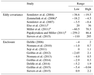
∗ Results were reported as a range of daily averages (5 h average in the case of Papakyriakou and Miller, 2011). Full measurement ranges are necessarily larger, though unreported.
Over the last several decades the two main approaches for measuring over sea ice have been the enclosure method and the eddy covariance (EC) method. The enclosure method works by measuring the change in gas concentration over time within a chamber placed on the sea ice (Miller et al., 2015). The main shortcoming with this method is that it alters the environment which is being measured (e.g., affecting temperature, radiation, pressure gradients, wind speed and turbulence, and atmosphere–surface CO2 concentration differences). Proper technique can minimize these artifacts, but even under the best conditions it is expected that they will cause some underestimation of (Miller et al., 2015). Additionally, the measurements are spatially and temporally limited. Measurements are confined to the region enclosed by the chamber (centimeter scale), making it challenging to accurately measure fluxes over whole ecosystems (meter to kilometer scale), which typically contain heterogeneity on scales larger than the footprint of the chamber. Additionally, long-term measurements are not feasible for enclosures due to the fact that they alter the underlying environment and the degree of manual intervention they require.
The EC technique works by measuring vertical wind speed and gas concentration at high frequencies. The covariance between fluctuations in vertical wind and fluctuations in the gas concentration, averaged over a period of time, represents a direct measurement of flux. Unlike the enclosure method, it does not alter the environment in which it measures and is practical for gathering long-term continuous measurements of flux over a spatial scale that encompasses the natural heterogeneity of sea ice.
The enclosure and EC methods have not shown good agreement over sea ice, for which flux magnitudes measured by EC systems have been consistently higher than those measured by enclosures (Table 1). Over landfast sea ice the enclosure method produces fluxes on the order of −5.4 to 2.2 mmol m−2 d−1 (Delille, 2006; Nomura et al., 2010, 2013; Sejr et al., 2011; Geilfus et al., 2012, 2014, 2015; Delille et al., 2014; Sievers et al., 2015), while EC often measures uptake and effluxes of several hundred mmol m−2 d−1 (Miller et al., 2011; Papakyriakou and Miller, 2011; Sievers et al., 2015). Fluxes of this magnitude are suspiciously high. They compare in magnitude with terrestrial fluxes (Christensen et al., 2000; Lafleur et al., 2003; Sullivan et al., 2008) and fluxes over open-ocean algal blooms (Yang et al., 2016a).
The most likely explanation for the large discrepancy between methods is a failure of the open-path infrared gas analyzer (IRGA) used in the EC systems. Overestimation of by open-path EC in the low-flux marine environment has been documented as far back as Broecker et al. (1986), and has since been confirmed (Miller et al., 2010; Blomquist et al., 2014; Landwehr et al., 2014). Closed-path eddy covariance systems may reduce measured magnitude (e.g., Sievers et al., 2015 measured a mean of 1.73±5 mmol m−2 d−1 over landfast sea ice), but have been shown to be affected by the same problems as the open-path IRGAs (Blomquist et al., 2014; Landwehr et al., 2014; Butterworth and Miller, 2016b). An improved technique was developed by Miller et al. (2010) which used a closed-path IRGA and dried sample airstream. This system addressed the problems with previous EC systems by eliminating fluctuations in all variables (pressure, temperature, and H2O) associated with the density correction (Webb et al., 1980). Subsequent studies have confirmed the effectiveness of this approach for measuring air–sea fluxes (Blomquist et al., 2014; Landwehr et al., 2014; Butterworth and Miller, 2016b; Bell et al., 2017).
Cavity ring-down spectroscopy (CRDS) may be suitable for measuring over landfast sea ice, though it has yet to be field tested. Open water results have confirmed flux detection limits for dried Picarro instruments (G1301-f; G2311-f) to be in the range needed for measuring over landfast sea ice (Blomquist et al., 2014; Yang et al., 2016b). The Los Gatos Research FGGA on the other hand (in which drying is less feasible) has flux detection limits that may not be suitable for measuring at the low flux magnitudes expected over landfast sea ice (Yang et al., 2016b), though Prytherch et al. (2017), using an undried FGGA, measured in the Arctic marginal ice zone that agreed with previous results (Butterworth and Miller, 2016a). Because CRDS systems are expensive and have significant power demands, systems based on closed-path IRGAs are currently more practical for making continuous flux measurements in Arctic environments.
For this study, we applied the dried, closed-path IRGA design to measure from a permanent tower over sea ice in the Canadian Arctic. This is the first EC system of this kind to measure over landfast sea ice. The benefits of a fixed tower are that it avoids the motion contamination and flow distortion associated with ship-based EC. Additionally, it is capable of collecting a long-term continuous flux dataset in one area, thus enhancing our ability to address process-level questions. Here we will present 4 months of flux data from the spring and summer season (May to September 2017) as the region transitioned from full ice cover to open water and describe the performance of the system. Our primary goal in this paper is to describe the design and performance of the system, while subsequent articles will more fully explore the insights gained about CO2 exchange in the sea ice environment.
2.1 Site description
An eddy covariance system to measure fluxes of momentum, sensible heat, latent heat, and CO2 was installed on a 10 m tower located on the northwest side of Qikirtaarjuk Island, a low-lying island (500×200 m) in Dease Strait, roughly 35 km west of Cambridge Bay, Nunavut (Fig. 1). Qikirtaarjuk Island is the southernmost island in a chain that extends across Dease Strait, creating active tidal straits that produce polynyas in the fall and early spring (Fig. 1). Except for the islands north of the tower, the closest being Unihitak Island 3.5 km away, the tower has unimpeded fetch on the order or 50 km from large-angled swaths to the east and west. This ensures that much of the flux footprint represents only water and not a mix of water and land.
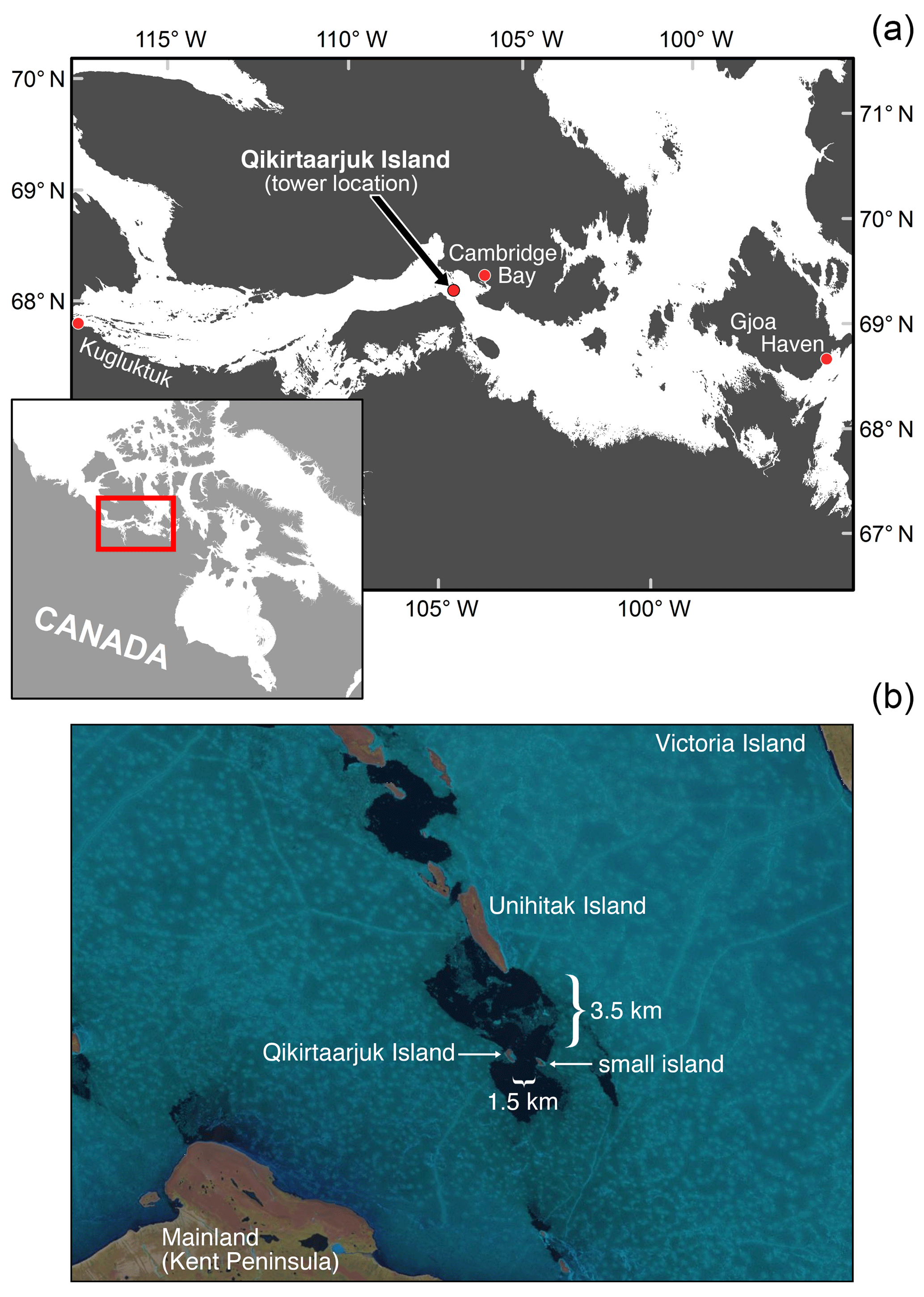
Figure 1Map (a) showing the location of Qikirtaarjuk Island, 35 km west of Cambridge Bay, Nunavut. Satellite image (b) of Qikirtaarjuk Island (28 June 2017), showing polynya development in the tidal straits. Landsat-8 image courtesy of the U.S. Geological Survey.
2.2 Instrument setup
The tower was configured with an array of instruments (Fig. 2) to measure mean meteorological variables (logged as 1 min averages on a Campbell Scientific CR1000 data logger) and high-frequency flux variables (10 Hz; CR3000 data logger). Mean wind speed and direction were measured using a 2-D propeller vane anemometer (RM Young; Marine Wind Monitor) mounted at 7.8 m above ground level (a.g.l.). Three temperature and relative humidity probes (Campbell Scientific HMP45C) were mounted at 9.6 m, 5 m, and 2.2 m a.g.l. A net radiometer (Kipp & Zonen; CNR4) was mounted 2.8 m a.g.l.
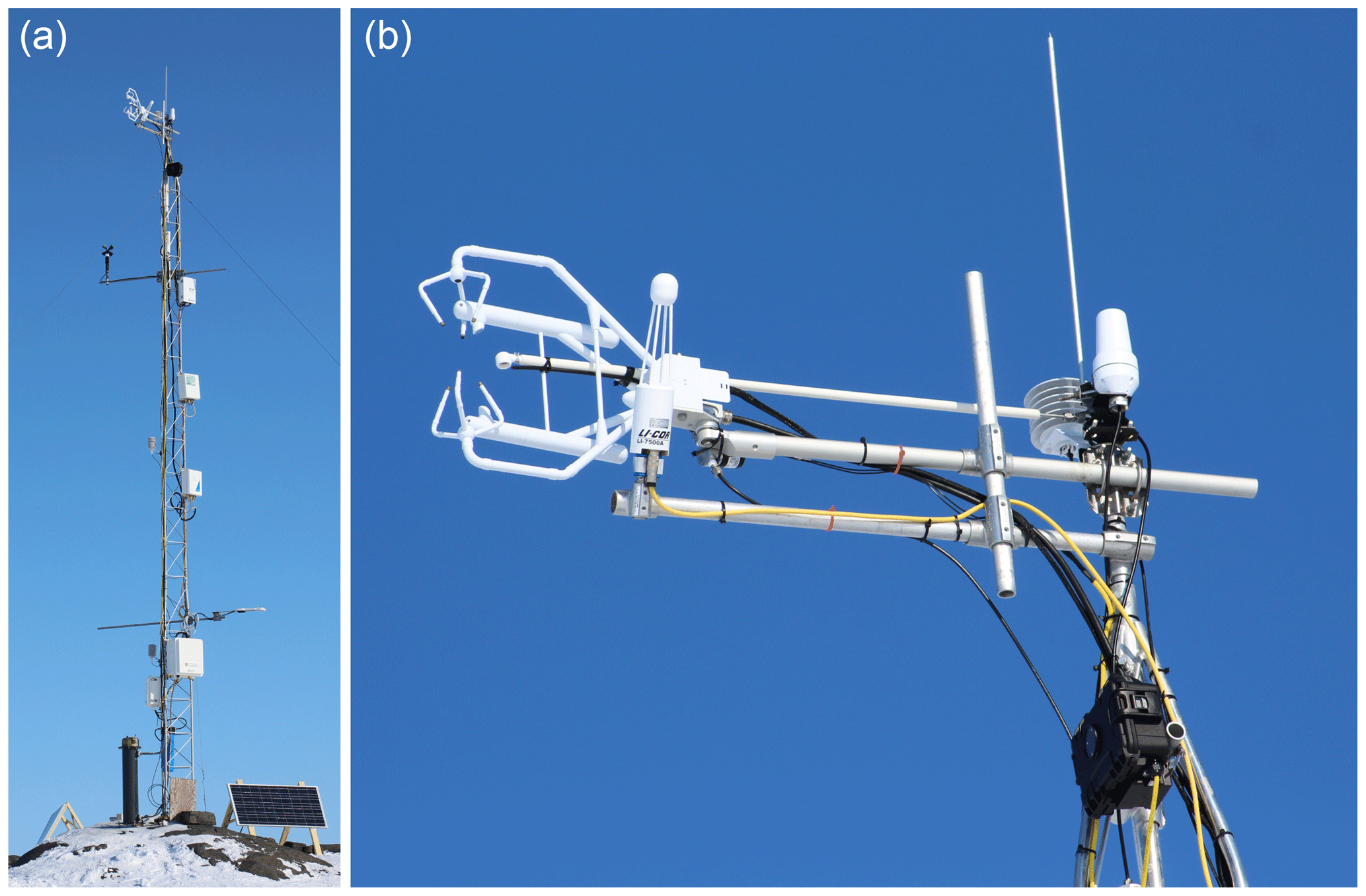
Figure 2Photograph of the tower (a) and the flux instruments mounted at the top of the tower (b).
2.2.1 Wind vector
Measurements of momentum and sensible heat fluxes were obtained using a 3-D ultrasonic anemometer (CSAT3; Campbell Scientific) mounted at 9.5 m a.g.l., oriented northwest (330∘), and roughly 15 m from the water's edge. The ground level at the tower base was roughly 3 m above mean sea level (a.s.l.), making the measurement height 12.5 m a.s.l. However, 3-D wind measurements show that the streamlines are directionally dependent and bend upward/downward in proportion to the island incline (a maximum of 6∘ from head-on winds). Therefore, wind and flux measurements were considered representative of 9.5 m a.s.l. (similar to vertical displacement seen in ship-based measurements; Yelland et al., 2002). For each 20 min flux interval a double rotation was applied on the wind vector to put it into a mean streamline coordinate system in which the x axis was parallel to the mean wind () (Kaimal and Finnigan, 1994).
2.2.2 H2O & CO2
Water vapor and CO2 concentrations used to calculate fluxes were measured by three IRGAs. Two were open-path designs (EC150, Campbell Scientific and LI-7500, LI-COR) and one was a closed-path design (LI-7200RS, LI-COR, referred to herein as LI-7200). The EC150 was attached to the CSAT3 anemometer, making its measurements collocated with the wind vector measurements. The LI-7500 was mounted 30 cm aft, 18 cm starboard, and at the same height as the CSAT3. Mixing ratios for the IRGAs were calculated from molar density, pressure, and temperature using the WPL correction (Webb et al., 1980). This was even done for the LI-7200 (using as suggested by LI-COR) because it was deemed more reliable than the LI-7200's on-the-fly calculation of mixing ratio, which inexplicably produced with large contributions from low frequencies.
Unlike the open-path IRGAs, the LI-7200 required a pump to pull air through its cell. As pumps significantly increase power requirements, this has been one of the barriers to closed-path IRGAs being used in remote Arctic EC towers. The sample air for the LI-7200 was drawn from an inlet 5 cm aft of the CSAT3 sampling volume. Ideally, flow through the LI-7200 should be fast enough to fully flush its cell every sample (9.7 standard liters per minute (slpm) for 10 Hz sampling). However, the maximum flow rate that could consistently be achieved by our 12V DC diaphragm pump (UN814KNDC, KNF) was 7 slpm. To ensure that flow remained constant, a mass flow controller (MCRW-10SLPM-D-DB9/5M, Alicat) was installed immediately upstream of the pump. It was expected that this flow rate should cause a minor loss of signal at the high-frequency end of the spectrum (evaluated below).
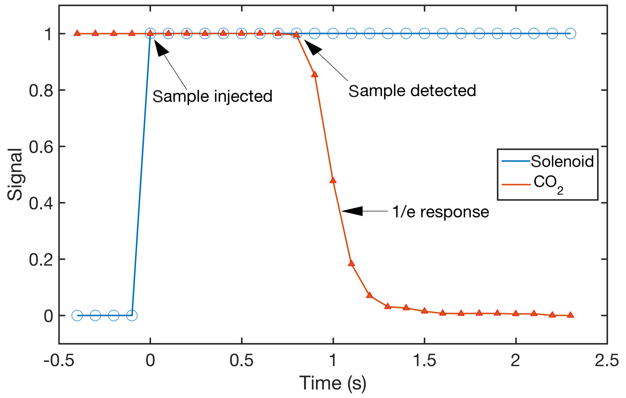
Figure 3Mean tube delay obtained from 574 inlet tests. Blue circles show the state of the solenoid valve (0 = closed; 1 = opened) responsible for releasing compressed N2 directly in front of the sample tube inlet to the closed-path IRGA. The red triangles represent the decay in the CO2 mixing ratio from its pre-test steady state (1) to its settled value during the test (0).
The mounting configuration of the LI-7200 was chosen to minimize signal attenuation by tubing. The diameter of the tubing upstream of the LI-7200 was minimized (3.5 mm I.D.) to increase the Reynolds number (Re). With 7 slpm flow Re in the sample line was 2800, in the transitional zone between laminar (Re < 2100) and turbulent (Re > 4000). To mitigate the signal smoothing that could occur with nonturbulent flow, the LI-7200 was mounted near the top of the tower, reducing upstream tube length to 2.8 m.
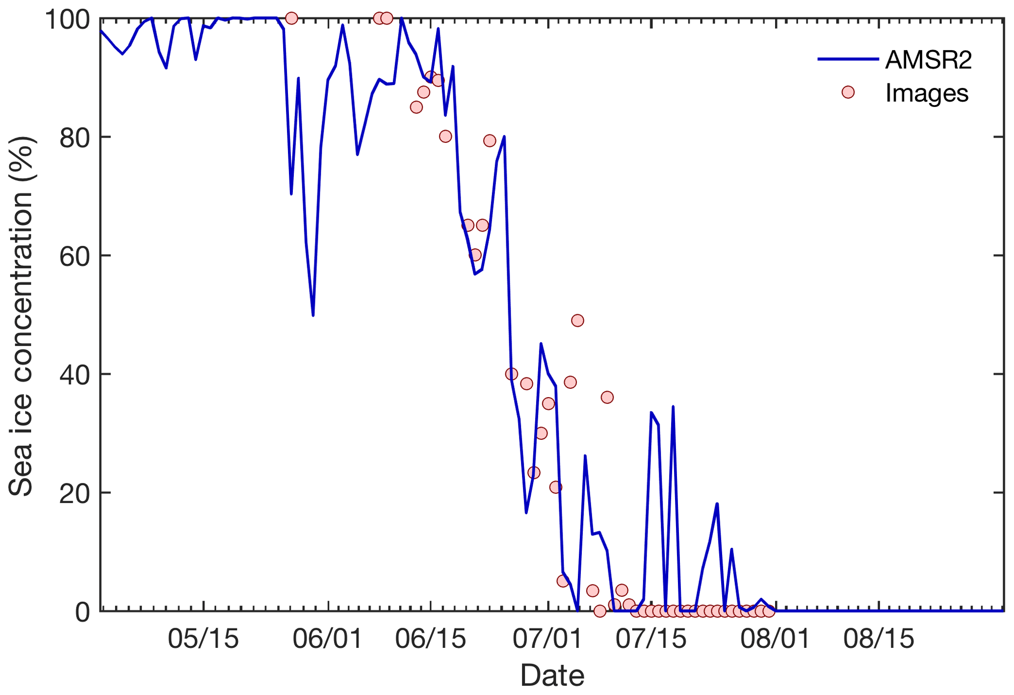
Figure 4Sea ice concentration from the AMSR2 SIC product and the mean daily average from satellite and in situ images.
To test for tube delay and attenuation of high-frequency signal, inlet tests with CO2-free air were performed regularly. Twice a day at 02:05 and 14:05 LST a normally closed, two-way solenoid valve installed at the base of the CSAT3 would open and inject nine 10 s pulses of N2 directly in front of the intake tube to the LI-7200. The mean delay for CO2 from 574 tests was 0.83±0.01 s (Fig. 3). The mean time constant (defined as the time for signal to drop below 1∕e strength) was 0.24±0.02 s. This time constant (less than three samples at 10Hz) was low and suggested minimal attenuation by the tubing. High-frequency loss of was characterized by estimating the flux lost by the open-path latent heat flux measurement after applying a low-pass filter to H2O mixing ratio using the CO2 time constant as a cutoff frequency (Goulden et al., 1996). The ratio (Gc) of unfiltered to filtered latent heat flux indicated an average high-frequency loss of 1.7 %, in line with previous studies (Ibrom et al., 2007; Butterworth and Miller, 2016b). To account for this loss, while reducing the variability in Gc, a linear regression between Gc and was calculated () and used to compute a multiplier for each flux interval based on the wind speed.
2.2.3 Sea ice
Images of sea ice were captured by a camera (Hero4, GoPro) mounted at the top of the tower. An intervalometer was installed to take a picture once an hour, indefinitely. These images were to be used to determine sea ice concentration (SIC) and melt pond fraction. However, the external battery packs for the camera failed late May 2017, and no images were collected by the camera until the issue was fixed mid-July 2017. Because of this, we relied on several other methods for estimating SIC. The AMSR2 passive microwave SIC product (daily, 3.125 km) by the University of Bremen (Spreen et al., 2008) was used to provide a picture of the seasonal ice breakup of the area. The ice concentration from the three grid cells nearest the tower were averaged. In addition to this product a variety of remotely sensed (Landsat-8 and MODIS) and in situ images were collected. In situ photographs were taken during site visits (four helicopter trips in June and July) and from a motion-sensor-equipped trail camera (installed to identify wildlife interactions with the installation, e.g., Fig. S1 of the Supplement, but which was frequently set off by environmental conditions). Comparisons between the AMSR2 SIC product and photographs confirms that it was generally accurate within the Dease Strait region (Fig. 4), with the exception that it could not resolve melt ponds as different from open water. This meant that during the melt pond season (June) the product underestimated SIC due to the presence of overlying water. Combining the photographs with the SIC product enabled estimates of melt pond fraction. Additionally, the AMSR2 product continued to measure SIC in mid-July, after images revealed full open water in front of the tower (Fig. 4). This discrepancy was due to the fact the AMSR2 product had a footprint that extended beyond the immediate area in front of the tower (which turns to open water more quickly than the rest of the region).
2.2.4 Power
Power limitations often exert a large influence on experimental design in Arctic field studies. With a closed-path IRGA and airstream drying, this study required two pumps and a mass flow controller, and needed roughly 4 times the power required by an open-path system. With no external power to draw from, all power needed to be generated on site. Three 150W solar panels (EWS-150P-36, Enerwatt) and one 12V DC wind turbine (AIR Breeze, Primus) were used to generate power that was stored in a battery bank of five 92AH AGM batteries. The battery bank was housed in a large Pelican case, and included charge controllers and circuit breakers for both the solar panels (30A 12VDC EWC-30, Enerwatt) and turbine (Wind Control Panel, Primus). The solar panels were arranged in a triangular formation to collect solar radiation at different times throughout the long summer days. The turbine was used as supplemental power to enable power generation when solar panels were not active (night and winter). To conserve power the flux system was design to shut off the more power-hungry equipment (gas analyzers, mass flow controller, DC pumps, and sonic anemometer) when voltage in the battery bank dropped below 11.8 V, and turn them back on again when voltage rose above 12.3 V. The system was fully operational 99.2 % of the time during the study period. A schematic diagram (Fig. S2) of the power system is included in the Supplement.
2.2.5 Drying
Like previous dried airstream systems, our system used a moisture exchanger (Nafion PD-200T-12MPS, Permapure) to dry the sample air. However, instead of a using a zero-air generator for purging water vapor from the counterflow (which would have required AC power and compressed air), a desiccant (Du-Cal Drierite) was used. Air was pumped (UN814KNDC, KNF) in a closed loop through a large cylindrical tank containing 50 lbs. of desiccant, to the moisture exchanger, and back to the tank. The advantage of using a closed loop design is that the only moisture exposed to the desiccant was that which had passed through the moisture exchanger membrane. This, along with the large mass of desiccant, meant that the replacement of desiccant was required only once every 40–60 days, depending on ambient humidity. The need for desiccant replacement was determined with a small amount (1 lb.) of Indicating Drierite (which changes color when exhausted) placed by a glass window on the tank.
2.3 Data processing
Fluxes of momentum (τ, N m−2), sensible heat (HS, W m−2), latent heat (HL, W m−2), and CO2 (, mmol m−2 d−1) were calculated for 20 min intervals as
where u,v, and w (m s−1) are the along-wind, cross-wind, and vertical wind components, respectively, (mol m−3) is the mean dry air density, cp (J kg−1 K−1) is the specific heat capacity of air, T (K) is the dry air temperature, Lv (J kg−1) is the latent heat of vaporization, q (kg kg−1) is the specific humidity, c is the CO2 mixing ratio (µmol mol−1), primes indicate fluctuations about the mean, and the overbar corresponds to the time average. The dry air temperature was calculated from the sonic temperature after correction for the effect of water vapor on air density and speed of sound (Schotanus et al., 1983).
The mean wind speed from the sonic anemometer was adjusted to neutral stability at 10 m height using a semilogarithmic wind profile and assuming a constant flux layer according to
where is the friction velocity (m s−1) measured by CSAT3, κ is the von Karman constant of 0.4, z is the measurement height, and z0 is the roughness length (m) calculated as
where ψm represents the stability function of Paulson (1970) for unstable stratification and Grachev et al. (2007) for stable stratification, both functions of z∕L, where z is the measurement height and L is the Obukhov length, calculated as
where g is the acceleration due to gravity, T is the air temperature, Q is the specific humidity, and and are the turbulent fluxes of temperature and water vapor (Andreas et al., 2010).
Quality control criteria were used to select intervals that passed the underlying assumptions of eddy covariance. First, intervals were selected that exhibited stationarity, following
where represents the mean of the four 5 min turbulent flux subintervals and represents the turbulent flux of the whole 20 min interval (Blomquist et al., 2014). The purpose of this criterion is to identify and remove intervals in which large-scale phenomena (e.g., mesoscale motions), outside the frequency range of turbulent fluxes, are contributing to the measured flux.
A second quality control criterion selected for wind directions of −150 to 150∘ (relative to the anemometer) to eliminate winds from aft that were affected by flow distortion from the instruments and tower frame. The size and shape of the island (0.2 km wide and extending 0.5 km behind the tower) meant the remaining wind directions from the back hemisphere had some degree of island contributing to their flux footprint. To estimate the impact of the island on the flux measurements, we ran the flux footprint model of Kljun et al. (2015). Using the mean meteorological conditions from each 5∘ wind sector it was found that on average the island accounted for 5 % of the footprint for wind directions from the front hemisphere (−90 to 90∘). From the back wind sectors (−150 to −90∘ and 90 to 150∘) 44 % of the flux footprint was represented by the island. However, because extent of the footprint varied with meteorological conditions, there were many periods during which these wind directions saw minimal influence from the island. The island is bare rock, which means that it should not act as either a source or a sink for CO2. This means that the magnitudes of CO2 fluxes from these back sectors are somewhat underestimated, by a factor that most likely scales with the portion of the footprint that falls on the island. Future work is planned to collect field data (i.e., coincident upwind pCO2w data for varying wind directions) to determine if a linear scaling factor could be used to correct flux magnitudes for these wind sectors.
2.3.1 Low-frequency contribution
One issue that was encountered during flux processing was unexpected low-frequency (between 10−3 to 10−2) contribution to , separated from contributions from the typical frequency range for turbulent fluxes by a distinct spectral gap (Fig. 5a). The spectral gap suggests that the low-frequency contributions were the result of larger scale motions (e.g., advection) and not representative of locally meaningful fluxes. To remove this from the flux measurements a high-pass filter (first-order Butterworth filter with cutoff frequency of 0.005 Hz centered on the trough in the spectral gap) was applied to the CO2 mixing ratio prior to calculating . This reduced magnitude by an average of 15.8 % (or 0.6 mmol m−2 d−1; Fig. 5a). The choice to filter had to balance the need to remove spurious flux with the possible removal of real flux operating at lower frequencies (Sakai et al., 2001; Finnigan et al., 2003). To assess the loss of real flux we applied the same high-pass filter to T and calculated HS. Filtering caused an average flux loss of 3.5 %, represented in Fig. 5b as the area between the unfiltered and filtered HS cospectra. This real flux loss is substantially less than that lost by filtering , which indicates that the filtering was appropriate in this instance. Future investigations into the processes affecting (e.g., melt pond fraction, sea ice concentration) would benefit from a more subjective review of cospectra for individual flux intervals. Because is presented more broadly in this paper, that level of scrutiny is not warranted here.

Figure 5Median normalized frequency-weighted cospectra for (a) and HS (b). In (a) the purple line represents the cospectrum calculated from the uncorrected LI-7200 CO2 mixing ratio. The green curve represents the cospectrum calculated from the high-pass-filtered LI-7200 CO2 mixing ratio. The dashed gray line represents the theoretical scalar cospectra from Kaimal et al. (1972). In (b) the blue curve represents the cospectrum for HS calculated from an unfiltered air temperature measurement. The red curve represents the cospectrum for HS calculated from air temperature passed through the same high-pass filter applied to the CO2 mixing ratio in the calculation (i.e., first-order Butterworth filter with 0.005 Hz cutoff). The area below the shaded region between the two curves represents the median loss of real low-frequency flux due to filtering.
3.1 Meteorology
The period reported in this study ranges from 4 May to 1 September 2017, encompassing the transition from full ice coverage to fully open water. From 4 May through 25 May the study area was characterized by snow-covered sea ice. With air temperatures well below 0 ∘C, this period represents winter ice conditions. From 25 May to 25 June melt ponds began to form. Comparing the AMSR2 SIC product to the in situ photographs (which show no open water) suggests that the melt ponds during this period ranged from 0 to 50 % of the surface area. Following this period there was an ice breakup period (25 June to 7 July) which exhibited both ice and open water. This breakup initially occurred directly in front (north) of the tower, creating a polynya that was probably caused by tidal currents in the strait funneled between the islands (Fig. 1). By the end of the breakup period the area was ice-free for the remainder of the summer season.
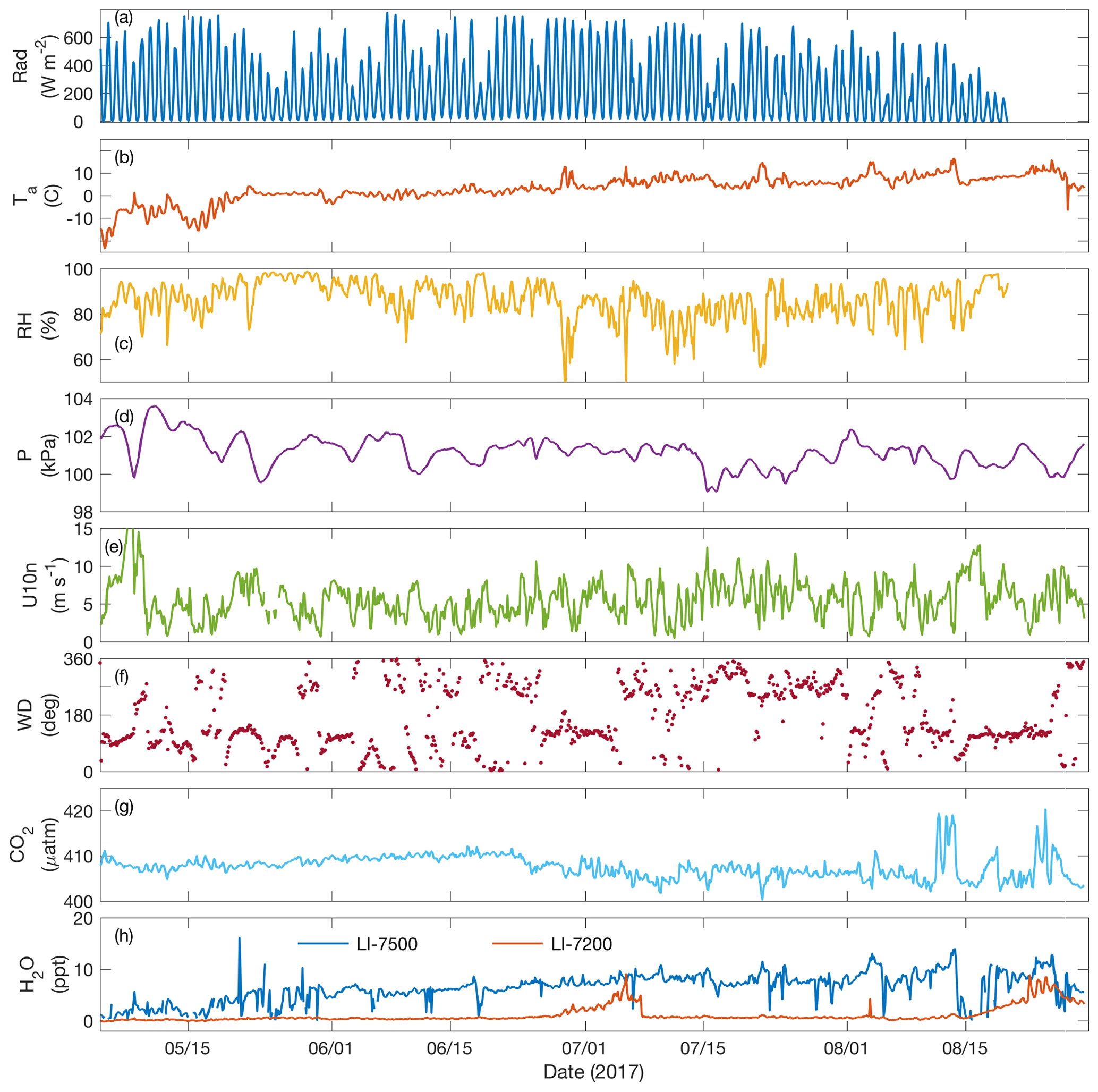
Figure 6Meteorological conditions from May to September 2017 shown as 3 h averages for (a) incoming solar radiation (W m−2), (b) air temperature (∘C), (c) relative humidity (%), (d) atmospheric pressure (kPa), (e) wind speed (m s−1), (f) wind direction (∘), (g) CO2 mixing ratio (ppm), and (h) water vapor concentration (ppt).
The meteorology of the study area through the study period shows the strong seasonal shift. The temperature over this period rose from its minimum of −24 ∘C on 5 May, to its maximum of 18 ∘C on 13 August, with over half of the time in between being within of 0 ∘C (Fig. 6b). Incoming solar radiation exhibited strong diurnal trends, with over 75 % of days experiencing peak daytime values greater than 500 W m−2, and nighttime minimum values near zero (Fig. 6a). These oscillations did not result in large diurnal temperature swings. Due to the low temperatures, the relative humidity was typically high, with a mean of 86 % (Fig. 6c). Actual water vapor content of the air was lowest in May, with a mean of 3.3 parts per thousand (ppt), followed by a mean of 7.7 ppt from June to September (Fig. 6h). The CO2 mixing ratio was roughly 410 ppm at the start of May and decreased to 403 ppm by the end of August, indicative of the seasonal trend that occurs when plant biomass consumes atmospheric CO2 in the boreal growing season (Fig. 6g). Wind speed was moderate, ranging between 0 and 16.4 m s−1 with a mean of 5.6±2.7 m s−1. The winds exhibited no distinct change in magnitude over the course of the season (Fig. 6e), and were most commonly from the southeast (105 to 135∘) and the west southwest (235 to 275∘) (Figs. 6f, 7). These directions were generally advantageous due to the large fetch in the east and west directions, the only caveat being the very small island 1.5 km southeast of the tower.
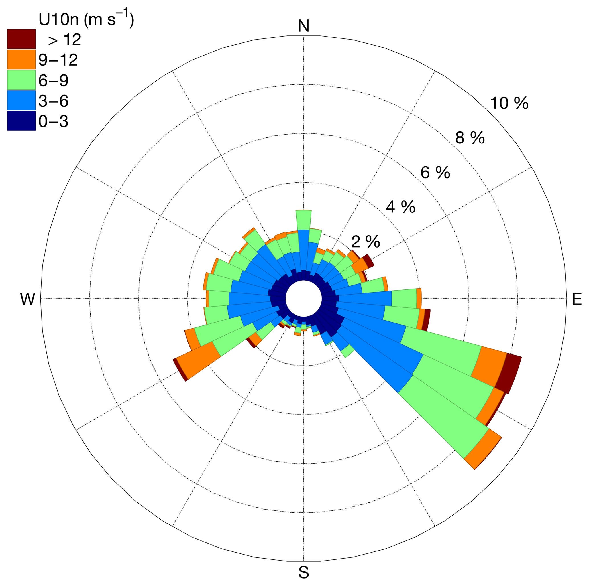
Figure 7Wind rose for May to September 2017 shown with 10∘ wind direction bins. Color represents 10 m neutral wind speed and the size of the bars indicates the frequency at which they occur.
3.2 Air–sea fluxes
Time series of τ, HS, HL, and over the course of this study are shown in Fig. 8. The τ ranged from 0 to 0.41 N m−2, with a mean of 0.05±0.05 N m−2 (Fig. 8a). The range in τ was similar through all different surface conditions, being most strongly influenced by wind speed. The HS showed a diurnal trend (increasing during the day, decreasing at night) throughout much of the study period. The sea surface type also played a role in mean HS, with the flux during full ice cover generally upward, then, during ice breakup and early summer downward, and in the open water at the end of the summer upward again. HL acted similarly to HS, with upward fluxes early in the season (full ice and melt ponds), transitioning to downward fluxes during ice breakup, and upward fluxes under full open water conditions.
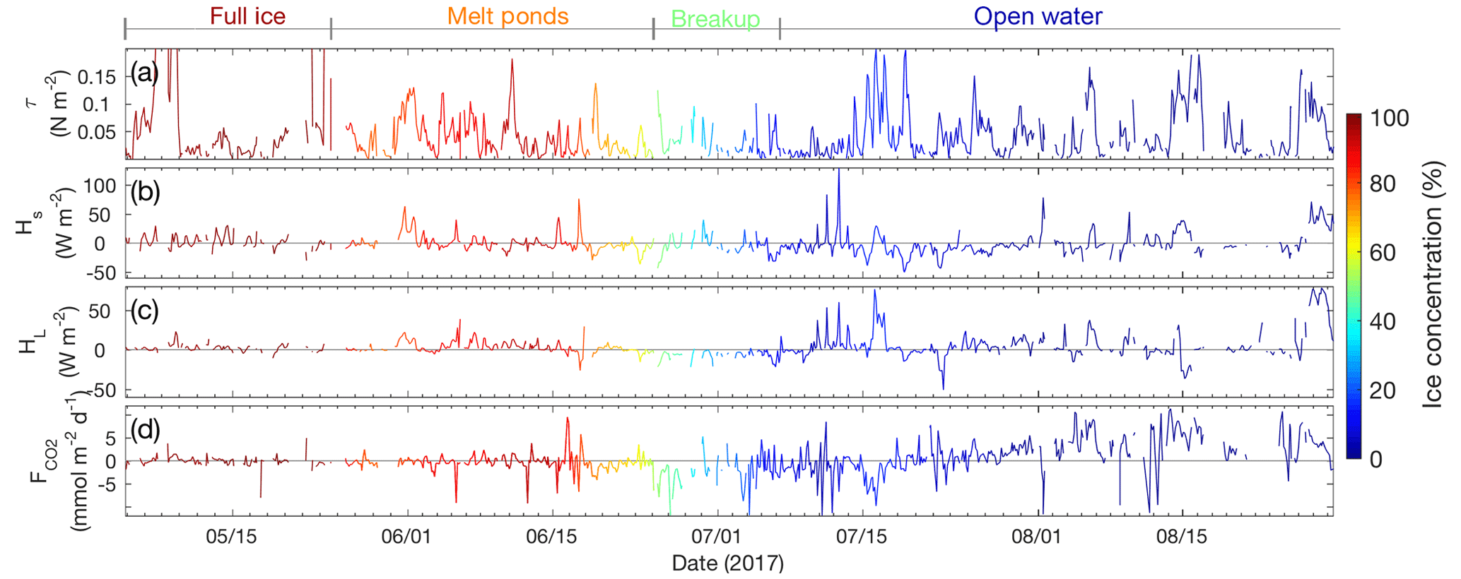
Figure 8The 3 h averages of measured fluxes, following the meteorological conventions (negative fluxes indicate transport towards the surface): (a) momentum flux (N m−2), (b) sensible heat flux (W m−2), (c) latent heat flux (W m−2), and (d) CO2 flux (mmol m−2 d−1), measured by the closed-path IRGA. Ice concentration from the AMSR2 ice product is shown by color, with red representing full ice cover and blue representing open water. Demarcations (determined from satellite and in situ images) of ice regimes (full ice, melt ponds, breakup, and open water) are shown on top.
3.3 CO2 flux
measured by the dried, closed-path system was low during periods with sea ice cover. During full ice cover hovered around zero, with a mean of mmol m−2 d−1. During melt season was slightly negative (i.e., downward), with a mean of mmol m−2 d−1. During ice breakup, when the surface was mixed ice and water, was downward (mean of mmol m−2 d−1). By the full open water period in August, had switched direction and the water was outgassing CO2 to the atmosphere (mean of 3.8±4.7 mmol m−2 d−1).
values calculated from the different IRGAs are shown in Fig. 9. Both open-path IRGAs yielded flux values with magnitudes much larger than those from the dried LI-7200, sometimes orders of magnitude larger. For example, during full ice conditions, when the dried LI-7200 measured near-zero , the LI-7500 and EC150 had means of and mmol m−2 d−1, respectively.

Figure 9The 12 h average CO2 fluxes calculated using EC150 (green diamonds), LI-7500 (blue pluses), and dried LI-7200 (red line). Demarcations (determined from satellite and in situ images) of ice regimes (full ice, melt ponds, breakup, and open water) are shown on top.
Because comparisons of from different gas analyzers do not have a dependent variable, we used Pearson's correlation coefficient (r) to describe the linear correlations between the two variables (Goodrich et al., 2016). Comparisons of from the closed-path LI-7200 against from the two open-path IRGAs showed no correlation (Fig. 10a, b), with r=0.04 and r=0.15 for the LI-7500 and EC150, respectively. An orthogonal regression of (LI-7500) against (EC150) yielded a fit closer to 1 : 1 (Fig. 10c), but with more scatter and an r=0.44. On the other hand, the regression for HL (LI-7500) against HL (EC150) showed a distinct 1 : 1 relationship (Fig. 10d). The correlation coefficient for this case was 0.93, thus showing a strong linear relationship. This suggests that the open-path IRGAs are better suited to measuring HL than in this environment.
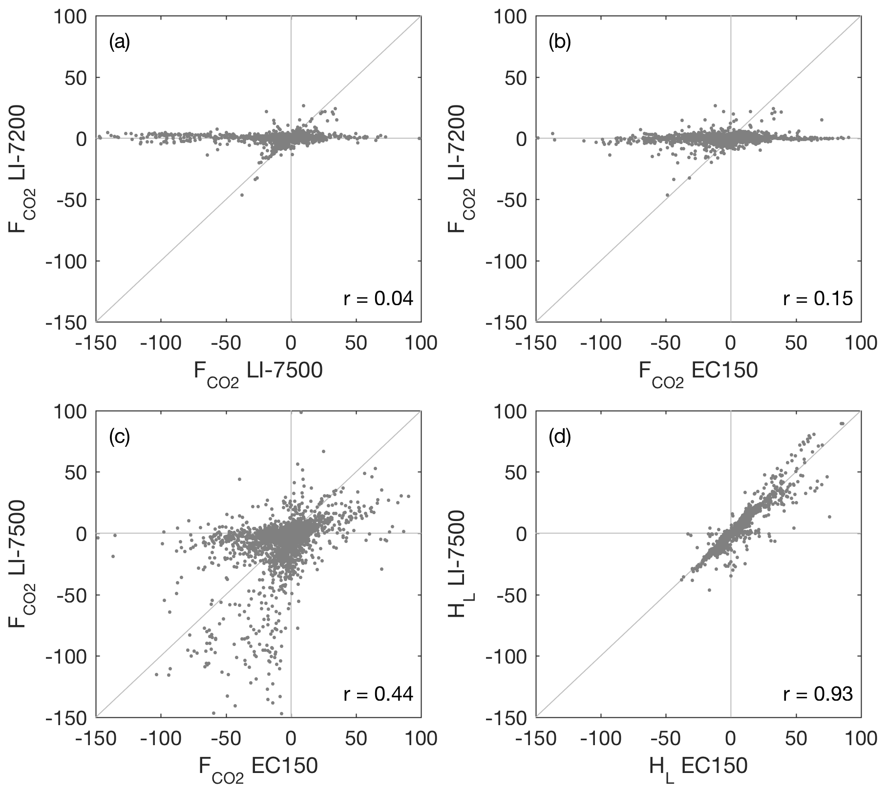
Figure 10Comparisons of and HL from the three IRGAs: panel (a) shows (LI-7200) vs. (LI-7500), panel (b) shows (LI-7200) vs. (EC150), panel (c) shows (LI-7500) vs. (EC150), and panel (d) shows HL (LI-7500) vs. HL (EC150). Because the sample air to the LI-7200 was dried, comparisons to HL (LI-7200) were omitted.
values from all three IRGAs were also compared against heat fluxes, HL and HS (Fig. 11). Negative relationships were found between from the open-path IRGAs and heat fluxes. from the dried, closed-path IRGA showed no relationship with HL or HS.

Figure 11Bin averages of the relationships between calculated from all three IRGAs and (a) HL (LI-7500) and (b) HS.
4.1 Sea ice flux comparisons
During the spring season prior to ice breakup, the dried, closed-path EC system measured of mmol m−2 d−1. When only considering sea ice conditions prior to melt pond formation, was mmol m−2 d−1. These measurements are within the range measured by previous enclosure measurements, which taken together span from −5.4 to 2.2 mmol m−2 d−1 (Table 1; Delille, 2006; Nomura et al., 2010, 2013; Sejr et al., 2011; Geilfus et al., 2012, 2014, 2015; Delille et al., 2014; Sievers et al., 2015). The measurements also exhibit a sharp divergence from previous open-path EC measurements, which at tens to hundreds of mmol m−2 d−1 are several orders of magnitude larger (Semiletov et al., 2004; Zemmelink et al., 2006; Else et al., 2011; Miller et al., 2011; Papakyriakou and Miller, 2011). Unlike the dried, closed-path system, our open-path systems installed at our site did measure with similar magnitudes to these previous open-path EC studies, with mean values of (LI-7500) and (EC150) mmol m−2 d−1.
This disagreement between simultaneous open-path and dried, closed-path systems at our site suggests that the reason for discrepancies between previous chamber and open-path EC measurements was not the result of different scales of measurement, but was rather problems with the ability of open-path EC to resolve fluxes. This is further demonstrated by the poor agreement between the two open-path results (Fig. 10c).
4.2 Heat fluxes
Previous undried EC studies over the open ocean have found relationships between heat fluxes (HS and HL) and (Landwehr et al., 2014; Sievers et al., 2015). However, in these instances the magnitude of measured at high latent heat fluxes exceeds values calculated from bulk formula. In their comparison of dried and undried closed-path EC systems, Landwehr et al. (2014) concluded that such relationships represented bias, and did not result from real physical phenomena. They also found that the degree of bias was different for each individual IRGA instrument. While our OP IRGAs found a relationship between heat fluxes and our dried, closed-path system did not (Fig. 11). This supports the finding that these relationships represent bias, further evidence that open-path IRGAs do not fully remove the effects of HS and HL in the density correction and/or the instruments' built-in water vapor corrections.
4.3 EC150
To the best of our knowledge, this study is the first published test of the EC150 against the LI7500 in a marine environment. The two instruments produced similar HL (Fig. 10d), showing that both are capable instruments for measuring water vapor flux. When it came to , the EC150 values diverged from the dried, closed-path system to a similar degree as the LI-7500 (Fig. 10b). Like the LI-7500, the EC150 also showed a strong negative relationship between and both HS and HL (Fig. 11). These findings suggest that the EC150 is affected by the same problems that affect the LI-7500.
However, comparison between the EC150 and LI-7500 did not show strong agreement (Fig. 10c). It is possible that the disagreement between the two stems from differences in their design (e.g., the EC150 is not necessarily affected by the same instrument-induced HS as the LI-7500 (Burba et al., 2008) and presumably has a different set of equations accounting for water vapor cross sensitivity). But the overall spurious, high magnitudes for appear to stem from problems inherent to the open-path design. The EC150, like the LI-7500, appears to be more appropriate for use in regions with larger magnitude .
4.4 Gas transfer velocity
While measuring in the same range as chamber measurements shows that the method ameliorates problems associated with open-path systems, it alone is not a full accounting of measurement quality. To further assess the performance of the flux system, we compared our open water results against those from previous studies. To do this we calculated gas transfer velocity, a coefficient which describes the efficiency of gas transport across the air–sea interface. Gas transfer velocity is a more effective comparison than because it provides more context. It was calculated by setting our measured flux equal to the bulk CO2 flux formula ( ) and rearranging the equation to form
where k is the gas transfer velocity, s is the solubility of CO2 in seawater, and pCO2w and pCO2atm are the partial pressure of CO2 in water and the atmosphere, respectively (Wanninkhof and McGillis, 1999). While and pCO2atm were continuously measured by the EC system, s and pCO2w were not. They were however, measured aboard the research vessel (RV) Martin Bergmann, which made several courses past the island in August 2017. For the flux intervals that aligned temporally with these passes (all fully open water), we calculated k660 (k adjusted to a Schmidt number (Sc) of 660). The k660 values plotted against (Fig. 12) showed good agreement with previous parameterizations of k660 (Wanninkhof, 1992, 2014). Because the (RV) Martin Bergmann data showed that pCO2w had high temporal and spatial variability in this region, and because we only have three data points, this result should not be interpreted as a new functional form to the k vs. relationship. What it does indicate is that the dried, closed-path flux system is able to resolve within an expected range, based on previous results. Conversely, k660 values from the open-path IRGAs were not similar to previous findings. For these three intervals, the mean k660 was 247 cm h−1 for the EC150 and −28 cm h−1 for the LI-7500 (where negative represents counter-gradient flux). This provides additional evidence that the open-path IRGAs are not capable of resolving CO2 fluxes in this environment.
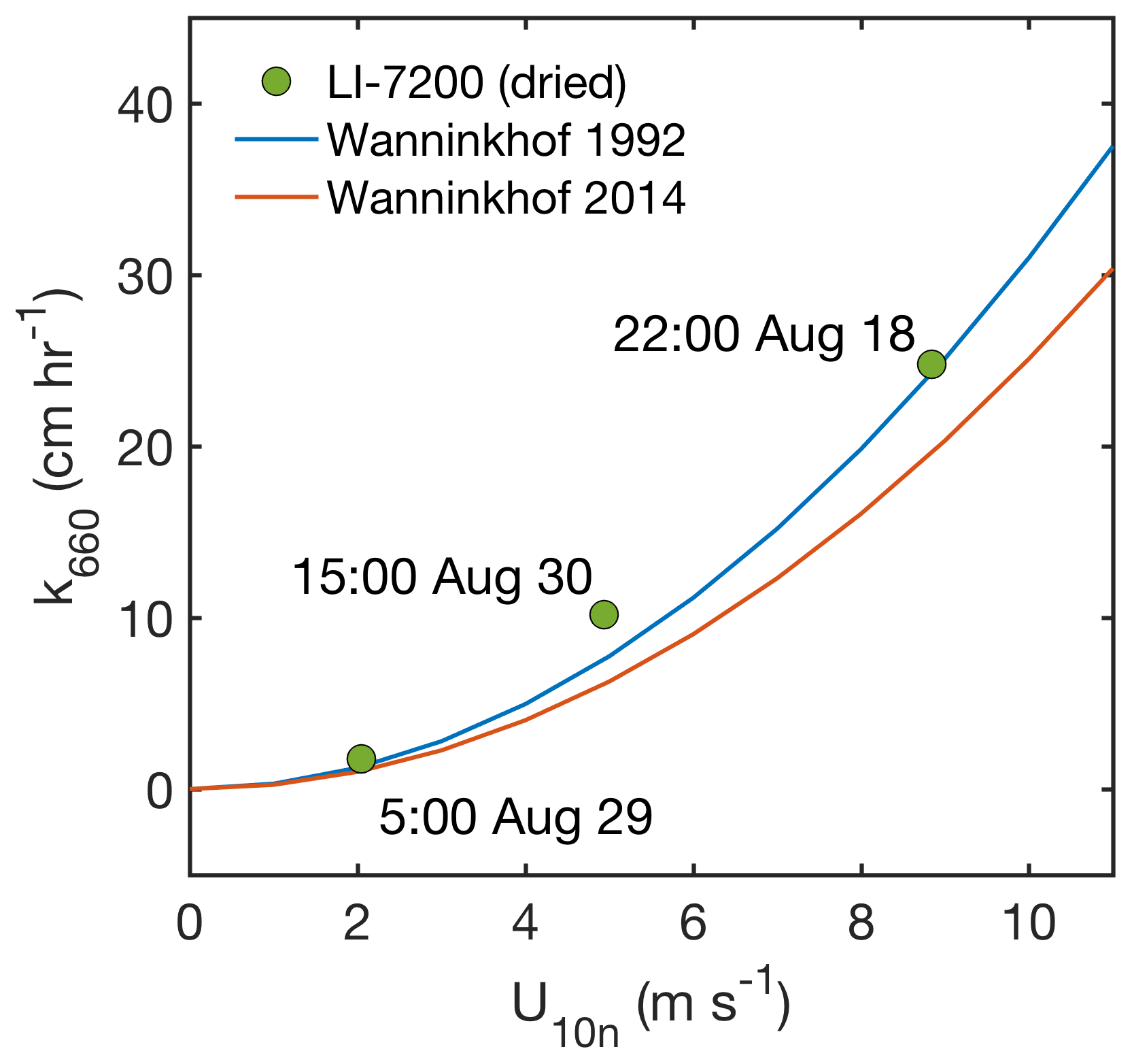
Figure 12Gas transfer velocity (k660) plotted against 10 m neutral wind speed for three periods in which the RV Martin Bergmann measured pCO2w within 3 km of the tower and in which the magnitude of ΔpCO2 (i.e., pCO2w−pCO2atm) was greater than 20 µatm. Parameterizations of Wanninkhof (1992) and Wanninkhof (2014) are shown as blue and red lines, respectively.
The quality of the flux measurement was also assessed by comparing previous years' measurements of pCO2w to estimated pCO2w (using ) from our study period. Measurements of pCO2w were collected aboard the Canadian Coast Guard (CCGS) Ice Breaker Amundsen near Qikirtaarjuk Island during five previous summers (2010, 2011, 2014, 2015, 2016). August measurements of pCO2w (collected within a 10 km radius of the tower) ranged from 360 to 469 µatm, with a mean of 407±34 µatm. Estimates of pCO2w from our study period were calculated by rearranging Eq. (9) so that pCO2w = k−1 s−1 + pCO2atm. As stated above, pCO2atm and were measured by the tower. Gas transfer velocity was obtained using the Wanninkhof (2014) parameterization with measured , plus the mean Schmidt number (Sc) from the RV Martin Bergmann dataset (Sc = 1150). Solubility was also estimated as the mean value from the RV Martin Bergmann data (s=48 mol m−3 atm−1).
Using from the dried, closed-path IRGA yielded pCO2w estimates ranging from 347 to 481 µatm (10th to 90th percentile) and a median value of 407 µatm, over the course of summer 2017. This matched reasonably well with the range identified by the CCGS Amundsen measurements. Comparatively, the pCO2w values from the open-path IRGAs were not as tightly clustered around a central value (Fig. 13). The fluxes from the LI-7500 and EC150 led to pCO2w estimates ranging from −1255 to 1101 µatm and −1252 to 906 µatm, respectively. These values are far beyond the magnitude observed in this region (and with no physical basis in the case of negative values), further evidence that the open-path IRGAs are not capable of providing accurate measurements in the relatively low ΔpCO2 conditions typically found in the marine environment.
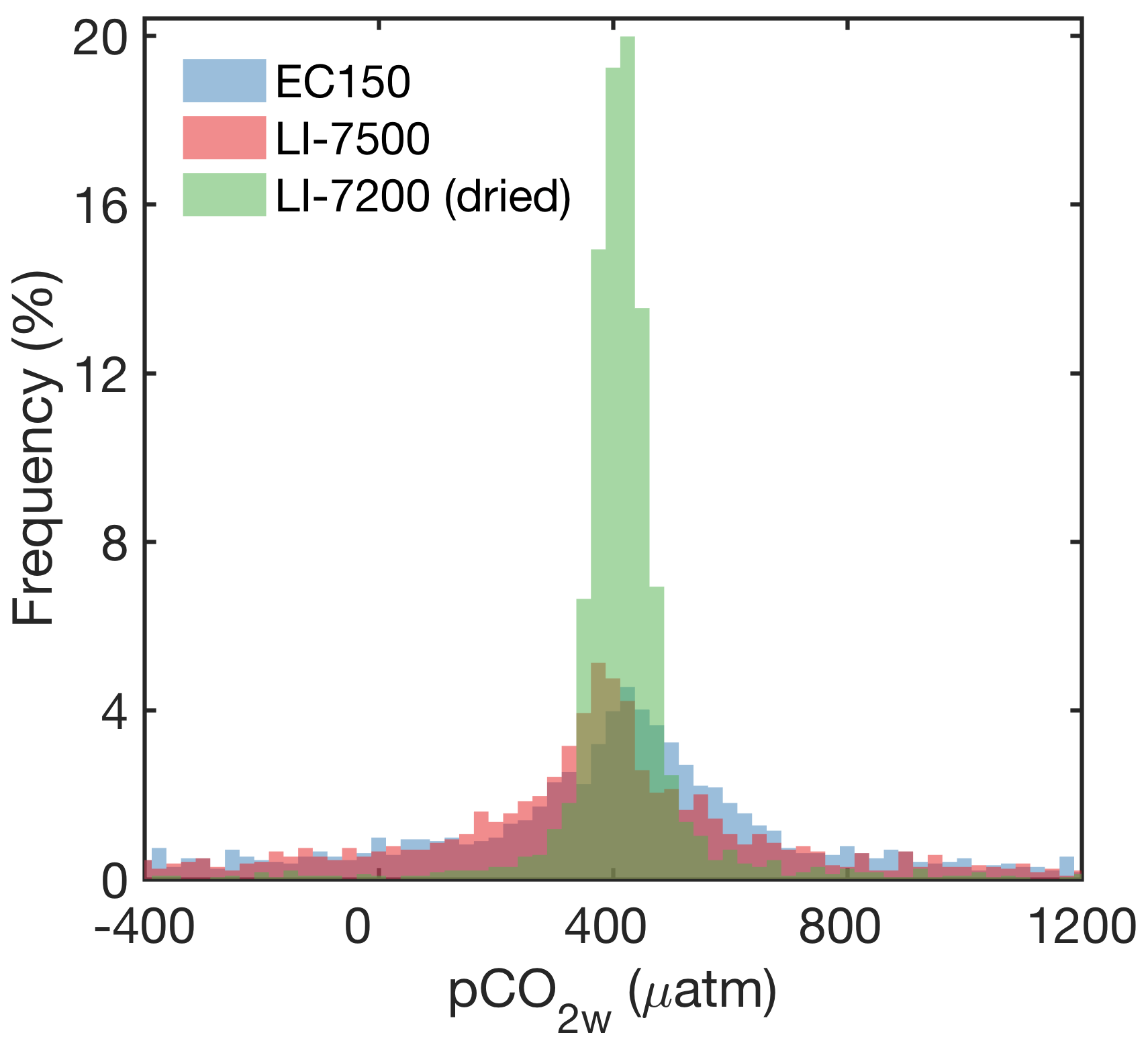
Figure 13Histograms showing the normalized frequency (%) of pCO2w calculated using from the EC150, LI-7500, and LI-7200. The limits in the x axis were truncated at −400 and 1200 for better visualization. However, roughly a quarter of pCO2w values from both the EC150 and LI-7500 extend beyond these limits.
4.5 Drying
The drying system worked as desired, drying the sample air to dew point temperatures of ∘C, compared to the LI-7500 which measured average ambient dew point temperatures of 6.0±7.6 ∘C. Perhaps more importantly it reduced fluctuations in water vapor, reducing the standard deviation in H2O mixing ratio by over an order of magnitude from 0.1±0.2 mmol mol−1 to 0.007±0.008 mmol mol−1. This resulted in reducing the standard deviation of the CO2 mixing ratio from 0.7±1.8 to 0.1±0.1 µmol mol−1. This matches the LI-7200's specification for root mean square noise at a sampling rate of 10 Hz, showing that preconditioning the sample air completely removed the influence of other variables on the CO2 measurement.
As the comparisons between the LI-7200 and LI-7500/EC150 show, drying the air did seem helpful in producing that are more in line with expected values. Interestingly, however, there were two occasions when the desiccant's capacity ran out and the closed-path IRGA was receiving sample air with near-ambient water vapor content (Fig. 6h). During those periods of time, the LI-7200 still experienced standard deviations in H2O mixing ratio 3.5 times lower than the open-path LI-7500. Additionally, there was no increase in the variance of from the LI-7200 during these periods, and magnitudes did not increase to open-path levels. This suggests that even without a dry counterflow, the Nafion drier still improves measurements to an acceptable level by reducing fluctuations in water vapor. This makes sense because spikes of moister or drier air will still exchange H2O with a counterflow that is at mean ambient humidity. Without a parallel, undried LI7200 it impossible to quantify how much of the smoothing is from the Nafion compared to the natural “stickiness” of H2O on tube walls. However, the impact of H2O smoothing from tube walls alone was tested in Butterworth and Miller (2016b) with an undried LI7200. It was found that tubing did not fully remove the influence of water vapor on the CO2 flux, and instead showed up as a spurious low-frequency contribution to the flux, which was visible in the flux cospectra. In this study, when the desiccant was exhausted, the cospectra did not indicate interference from water vapor, suggesting that the Nafion played a critical role. This finding may have important implications for the design of future systems (i.e., a system could be designed that uses a Nafion and counterflow, but without a dry air source), and should be investigated further.
4.6 Future work
In April 2018 as part of the Polar Knowledge Canada-funded CAT-TRAIN project in collaboration with the Arctic Research Foundation, a mobile power station/research lab was installed at the site. This new infrastructure will be used to increase the functionality of the system. Specific additions that are being considered are incorporating waterside pCO2w measurements, to be used to calculate gas transfer velocity continuously through an annual cycle. This would be particularly useful considering the pCO2w measurements from the CCGS Amundsen and the RV Martin Bergmann, which showed that this region often has ΔpCO2 of sufficient magnitude to measure accurate gas transfer velocities.
Additionally, for data redundancy we plan to install a second closed-path greenhouse gas analyzer (CRDS) capable of measuring CO2, H2O, and methane (GGA-FGGA, Los Gatos Research), which we which have only deployed on ships due to the large power consumption. Next spring a planned intercomparison study taking place in Cambridge Bay will add simultaneous enclosure measurements to verify agreement between the two methods. Lastly, the system will be used (in forthcoming papers) to investigate annual gas exchange cycles and process-level questions, including the processes affecting during spring melt and autumn freeze-up.
With its vast spatial extent, sea ice has the potential to play an important role in the global CO2 cycle. Unfortunately, there has been significant confusion around the importance of that role, largely because the community studying sea ice gas fluxes has been unable to reconcile large fluxes measured by eddy covariance with significantly smaller fluxes measured by enclosure methods (Table 1). This problem is analogous to the problem faced by researchers studying open water gas exchange, whereby for several decades EC measurements could not be reconciled with tracer-based measurements (e.g., Broecker et al., 1986). The open water problem was eventually resolved by using closed-path EC systems with a dried sample airstream (Miller et al., 2010), and EC measurements are now better aligned with other techniques.
The dried, closed-path IRGA method has previously been applied to the marginal ice zone (i.e., open water and drifting ice), where the open water likely dominates the CO2 flux signal (Butterworth and Miller, 2016a). In this study, for the first time we have applied sample drying techniques to an installation capable of measuring CO2 fluxes throughout an annual sea ice cycle. This allowed for measurements over many different surface conditions, including landfast sea ice, ice break-up, and open water. Fluxes measured during the open water season matched well with existing gas transfer parameterizations, lending credibility to the method. During the ice-covered season, this new measurement system closed the gap between EC and enclosure methods, producing with magnitudes in the range found by enclosure studies. This finding suggests that modeling or upscaling studies aiming to estimate the global CO2 exchange associated with landfast sea ice should focus on the smaller range of CO2 fluxes published by enclosure studies, at least until the EC method presented in this paper can be applied to more sea ice environments.
The dried, closed-path EC method presented here represents a significant advancement from previous attempts to measure over sea ice. We showed that incorporating the additional system complexity is feasible, even in remote polar locations, by presenting an effective approach for drying under low power requirements. The improved system can obtain long-term, continuous measurements over larger spatial scales than is possible with enclosures and opens potential avenues for new research, including a greater scrutiny of the ecosystem-scale processes affecting CO2 fluxes in sea ice regions.
The flux data from this study are not currently being placed in a data repository. We plan to publish the dataset as one full year of flux data with an upcoming paper highlighting the annual flux cycle.
The supplement related to this article is available online at: https://doi.org/10.5194/amt-11-6075-2018-supplement.
BJB and BGTE designed and installed the flux system. BGTE secured the grant funding for the research activities and organized field logistics. BJB processed and analyzed the flux data. BJB prepared the manuscript with contributions from BGTE.
The authors declare that they have no conflict of interest.
We wish to thank the many students and technicians who helped install and
maintain the eddy covariance tower, in particular Shawn Marriott, Patrick
Duke, Angulalik Pederson, Jasmine Tiktalek, Laura Dalman, and Vishnu Nandan.
Thanks are given to Yves Bernard for providing UAV footage. We would also like to
thank John Prytherch and an anonymous reviewer for their thoughtful
comments. The deployment of this tower in such a challenging location would
not have been possible without the excellent logistical support provided by
Polar Knowledge Canada, the Arctic Research Foundation, and the Polar
Continental Shelf Program. Financial support was provided by the Marine
Environmental Observation Prediction and Response (MEOPAR) Network of
Centres of Excellence, Polar Knowledge Canada, the Natural Sciences and
Engineering Research Council of Canada (NSERC), the Canada Foundation for
Innovation John R. Evans Leaders Fund, the Nunavut Arctic College, Irving
Shipbuilding Inc., and the University of Calgary. Special thanks are given to the
Ekaluktutiak Hunters & Trappers Organization for their continued support
of our projects and for the expert assistance provided by their guides.
This paper is a contribution to the SCOR Working Group 152 – Measuring
Essential Climate Variables in Sea Ice (ECV-Ice).
Edited by: Christian Brümmer
Reviewed by: John Prytherch and one anonymous referee
Andreas, E. L., Persson, P. O. G., Grachev, A. A., Jordan, R. E., Horst, T. W., Guest, P. S., and Fairall, C. W.: Parameterizing Turbulent Exchange over Sea Ice in Winter, J. Hydrometeorol., 11, 87–104, https://doi.org/10.1175/2009JHM1102.1, 2010.
Bell, T. G., Landwehr, S., Miller, S. D., de Bruyn, W. J., Callaghan, A. H., Scanlon, B., Ward, B., Yang, M., and Saltzman, E. S.: Estimation of bubble-mediated air–sea gas exchange from concurrent DMS and CO2 transfer velocities at intermediate-high wind speeds, Atmos. Chem. Phys., 17, 9019–9033, https://doi.org/10.5194/acp-17-9019-2017, 2017.
Blomquist, B. W., Huebert, B. J., Fairall, C. W., Bariteau, L., Edson, J. B., Hare, J. E., and McGillis, W. R.: Advances in Air-Sea CO2 Flux Measurement by Eddy Correlation, Bound.-Lay. Meteorol., 152, 245–276, https://doi.org/10.1007/s10546-014-9926-2, 2014.
Broecker, W. S., Ledwell, J. R., Takahashi, T., Weiss, R. F., Merlivat, L., Memery, L., Jähne, B., and Otto Munnich, K.: Isotopic versus micrometeorologic ocean CO2 fluxes: A serious conflict, J. Geophys. Res., 91, 10517–10527, https://doi.org/10.1029/JC091iC09p10517, 1986.
Burba, G., McDermitt, D. K., Grelle, A., Anderson, D. J., and Xu, L.: Addressing the influence of instrument surface heat exchange on the measurements of CO2 flux from open-path gas analyzers, Glob. Change Biol., 14, 1854–1876, https://doi.org/10.1111/j.1365-2486.2008.01606.x, 2008.
Butterworth, B. J. and Miller, S. D.: Air-sea exchange of carbon dioxide in the Southern Ocean and Antarctic marginal ice zone, Geophys. Res. Lett., 43, 7223–7230, https://doi.org/10.1002/2016GL069581, 2016a.
Butterworth, B. J. and Miller, S. D.: Automated underway eddy covariance system for air-sea momentum, heat, and CO2 fluxes in the Southern Ocean, J. Atmos. Ocean. Tech., 33, 635–652, https://doi.org/10.1175/JTECH-D-15-0156.1, 2016b.
Christensen, T. R., Friborg, T., Sommerkorn, M., Kaplan, J., Illeris, L., Soegaard, H., Nordstroem, C., and Jonasson, S.: Trace gas exchange in a high-arctic valley 1. Variations in CO2 and CH4 flux between tundra vegetation types, Global Biogeochem. Cy., 14, 701–713, https://doi.org/10.1029/1999GB001134, 2000.
Comiso, J. C., Meier, W. N., and Gersten, R.: Variability and trends in the Arctic Sea ice cover: Results from different techniques, J. Geophys. Res.-Oceans, 122, 6883–6900, https://doi.org/10.1002/2017JC012768, 2017.
Delille, B.: Inorganic carbon dynamics and air-ice-sea CO2 fluxes in the open and coastal waters of the Southern Ocean, Ph.D. thesis, Université de Liège, Liège, France, 2006.
Delille, B., Vancoppenolle, M., Geilfus, N.-X., Tilbrook, B., Lannuzel, D., Schoemann, V., Becquevort, S., Carnat, G., Delille, D., Lancelot, C., Chou, L., Dieckmann, G. S., and Tison, J.-L.: Southern Ocean CO2 sink: The contribution of the sea ice, J. Geophys. Res.-Oceans, 119, 6340–6355, https://doi.org/10.1002/2014JC009941, 2014.
Else, B. G. T., Papakyriakou, T. N., Galley, R. J., Drennan, W. M., Miller, L. A., and Thomas, H.: Wintertime CO2 fluxes in an Arctic polynya using eddy covariance: Evidence for enhanced air-sea gas transfer during ice formation, J. Geophys. Res., 116, C00G03, https://doi.org/10.1029/2010JC006760, 2011.
Finnigan, J. J., Clement, R., Malhi, Y., Leuning, R., and Cleugh, H. A.: Re-evaluation of long-term flux measurement techniques. Part I: Averaging and coordinate rotation, Bound.-Lay. Meteorol., 107, 1–48, https://doi.org/10.1023/A:1021554900225, 2003.
Geilfus, N.-X., Carnat, G., Papakyriakou, T. N., Tison, J.-L., Else, B. G. T., Thomas, H., Shadwick, E., and Delille, B.: Dynamics of pCO2 and related air-ice CO2 fluxes in the Arctic coastal zone (Amundsen Gulf, Beaufort Sea), J. Geophys. Res.-Oceans, 117, C00G10, https://doi.org/10.1029/2011JC007118, 2012.
Geilfus, N.-X., Tison, J.-L., Ackley, S. F., Galley, R. J., Rysgaard, S., Miller, L. A., and Delille, B.: Sea ice pCO2 dynamics and air–ice CO2 fluxes during the Sea Ice Mass Balance in the Antarctic (SIMBA) experiment – Bellingshausen Sea, Antarctica, The Cryosphere, 8, 2395–2407, https://doi.org/10.5194/tc-8-2395-2014, 2014.
Geilfus, N.-X., Galley, R. J., Crabeck, O., Papakyriakou, T., Landy, J., Tison, J.-L., and Rysgaard, S.: Inorganic carbon dynamics of melt-pond-covered first-year sea ice in the Canadian Arctic, Biogeosciences, 12, 2047–2061, https://doi.org/10.5194/bg-12-2047-2015, 2015.
Goodrich, J. P., Oechel, W. C., Gioli, B., Moreaux, V., Murphy, P. C., Burba, G., and Zona, D.: Impact of different eddy covariance sensors, site set-up , and maintenance on the annual balance of CO2 and CH4 in the harsh Arctic environment, Agr. Forest Meteorol., 228–229, 239–251, https://doi.org/10.1016/j.agrformet.2016.07.008, 2016.
Gosink, T. A., Pearson, J. G., and Kelley, J. J.: Gas movement through sea ice, Nature, 263, 41–42, https://doi.org/10.1038/263041a0, 1976.
Goulden, M. L., Munger, J. W., Fan, S. M., Daube, B. C., and Wofsy, S. C.: Measurements of carbon sequestration by long-term eddy covariance: Methods and a critical evaluation of accuracy, Glob. Change Biol., 2, 169–182, https://doi.org/10.1111/j.1365-2486.1996.tb00070.x, 1996.
Grachev, A. A., Andreas, E. L., Fairall, C. W., Guest, P. S., and Persson, P. O. G.: SHEBA flux–profile relationships in the stable atmospheric boundary layer, Bound.-Lay. Meteorol., 124, 315–333, https://doi.org/10.1007/s10546-007-9177-6, 2007.
Ibrom, A., Dellwik, E., Flyvbjerg, H., Jensen, N. O., and Pilegaard, K.: Strong low-pass filtering effects on water vapour flux measurements with closed-path eddy correlation systems, Agr. Forest Meteorol., 147, 140–156, https://doi.org/10.1016/j.agrformet.2007.07.007, 2007.
Kaimal, J. C. and Finnigan, J. J.: Atmospheric boundary layer flows: their structure and measurement, Oxford University Press, New York, 1994.
Kaimal, J. C., Wyngaard, J. C., Izumi, Y., and Coté, O. R.: Spectral characteristics of surface-layer turbulence, Q. J. Roy. Meteor. Soc., 98, 563–589, https://doi.org/10.1002/qj.49709841707, 1972.
Kljun, N., Calanca, P., Rotach, M. W., and Schmid, H. P.: A simple two-dimensional parameterisation for Flux Footprint Prediction (FFP), Geosci. Model Dev., 8, 3695–3713, https://doi.org/10.5194/gmd-8-3695-2015, 2015.
Kwok, R.: Near zero replenishment of the Arctic multiyear sea ice cover at the end of 2005 summer, Geophys. Res. Lett., 34, L05501, https://doi.org/10.1029/2006GL028737, 2007.
Lafleur, P. M., Roulet, N. T., Bubier, J. L., Frolking, S., and Moore, T. R.: Interannual variability in the peatland-atmosphere carbon dioxide exchange at an ombrotrophic bog, Global Biogeochem. Cy., 17, 1036, https://doi.org/10.1029/2002GB001983, 2003.
Landwehr, S., Miller, S. D., Smith, M. J., Saltzman, E. S., and Ward, B.: Analysis of the PKT correction for direct CO2 flux measurements over the ocean, Atmos. Chem. Phys., 14, 3361–3372, https://doi.org/10.5194/acp-14-3361-2014, 2014.
Maslanik, J. A., Fowler, C., Stroeve, J., Drobot, S., Zwally, J., Yi, D., and Emery, W.: A younger, thinner Arctic ice cover: Increased potential for rapid, extensive sea-ice loss, Geophys. Res. Lett., 34, L24501, https://doi.org/10.1029/2007GL032043, 2007.
Miller, L. A., Papakyriakou, T. N., Collins, R. E., Deming, J. W., Ehn, J. K., MacDonald, R. W., Mucci, A., Owens, O., Raudsepp, M., and Sutherland, N.: Carbon dynamics in sea ice: A winter flux time series, J. Geophys. Res.-Oceans, 116, C02028, https://doi.org/10.1029/2009JC006058, 2011.
Miller, L. A., Fripiat, F., Else, B. G. T., Bowman, J. S., Brown, K. A., Collins, E. R., Ewert, M., Fransson, A., Gosselin, M., Lannuzel, D., Meiners, K. M., Michel, C., Nishioka, J., Nomura, D., Papadimitriou, S., Russell, L. M., Sørensen, L. L., Thomas, D. N., Tison, J.-L., van Leeuwe, M. A., Vancoppenolle, M., Wolff, E. W., and Zhou, J.: Methods for biogeochemical studies of sea ice: The state of the art, caveats, and recommendations, Elem. Sci. Anthr., 3, 38, https://doi.org/10.12952/journal.elementa.000038, 2015.
Miller, S. D., Marandino, C. A., and Saltzman, E. S.: Ship-based measurement of air-sea CO2 exchange by eddy covariance, J. Geophys. Res., 115, D02304, https://doi.org/10.1029/2009JD012193, 2010.
Nomura, D., Eicken, H., Gradinger, R., and Shirasawa, K.: Rapid physically driven inversion of the air–sea ice CO2 flux in the seasonal landfast ice off Barrow, Alaska after onset of surface melt, Cont. Shelf Res., 30, 1998–2004, https://doi.org/10.1016/j.csr.2010.09.014, 2010.
Nomura, D., Granskog, M. A., Assmy, P., Simizu, D., and Hashida, G.: Arctic and Antarctic sea ice acts as a sink for atmospheric CO2 during periods of snowmelt and surface flooding, J. Geophys. Res.-Oceans, 118, 6511–6524, https://doi.org/10.1002/2013JC009048, 2013.
Papakyriakou, T. N. and Miller, L. A.: Springtime CO2 exchange over seasonal sea ice in the Canadian Arctic Archipelago, Ann. Glaciol., 52, 215–224, https://doi.org/10.3189/172756411795931534, 2011.
Paulson, C. A.: The Mathematical Representation of Wind Speed and Temperature Profiles in the Unstable Atmospheric Surface Layer, J. Appl. Meteorol., 9, 857–861, https://doi.org/10.1175/1520-0450(1970)009<0857:TMROWS>2.0.CO;2, 1970.
Prytherch, J., Brooks, I. M., Crill, P. M., Thornton, B. F., Salisbury, D. J., Tjernström, M., Anderson, L. G., Geibel, M. C., and Humborg, C.: Direct determination of the air-sea CO2 gas transfer velocity in Arctic sea ice regions, Geophys. Res. Lett., 44, 3770–3778, https://doi.org/10.1002/2017GL073593, 2017.
Sakai, R. K., Fitzjarrald, D. R., and Moore, K. E.: Importance of Low-Frequency Contributions to Eddy Fluxes Observed over Rough Surfaces, J. Appl. Meteorol., 40, 2178–2192, https://doi.org/10.1175/1520-0450(2001)040<2178:IOLFCT>2.0.CO;2, 2001.
Schotanus, P., Nieuwstadt, F. T. M., and de Bruin, H. A. R.: Temperature Measurement with a Sonic Anemometer and its Application to Heat and Moisture Fluxes, Bound.-Lay. Meteorol., 26, 81–93, https://doi.org/10.1007/BF00164332, 1983.
Sejr, M. K., Krause-Jensen, D., Rysgaard, S., Sørensen, L. L., Christensen, P. B., and Glud, R. N.: Air – sea flux of CO2 in arctic coastal waters influenced by glacial melt water and sea ice, Tellus, 63B, 815–822, https://doi.org/10.1111/j.1600-0889.2011.00540.x, 2011.
Semiletov, I. P., Makshtas, A., Akasofu, S.-I., and Andreas, E. L.: Atmospheric CO2 balance: The role of Arctic sea ice, Geophys. Res. Lett., 31, L05121, https://doi.org/10.1029/2003GL017996, 2004.
Semiletov, I. P., Pipko, I. I., Repina, I., and Shakhova, N. E.: Carbonate chemistry dynamics and carbon dioxide fluxes across the atmosphere – ice – water interfaces in the Arctic Ocean: Pacific sector of the Arctic, J. Marine Syst., 66, 204–226, https://doi.org/10.1016/j.jmarsys.2006.05.012, 2007.
Sievers, J., Sørensen, L. L., Papakyriakou, T., Else, B., Sejr, M. K., Haubjerg Søgaard, D., Barber, D., and Rysgaard, S.: Winter observations of CO2 exchange between sea ice and the atmosphere in a coastal fjord environment, The Cryosphere, 9, 1701–1713, https://doi.org/10.5194/tc-9-1701-2015, 2015.
Sitch, S., Friedlingstein, P., Gruber, N., Jones, S. D., Murray-Tortarolo, G., Ahlström, A., Doney, S. C., Graven, H., Heinze, C., Huntingford, C., Levis, S., Levy, P. E., Lomas, M., Poulter, B., Viovy, N., Zaehle, S., Zeng, N., Arneth, A., Bonan, G., Bopp, L., Canadell, J. G., Chevallier, F., Ciais, P., Ellis, R., Gloor, M., Peylin, P., Piao, S. L., Le Quéré, C., Smith, B., Zhu, Z., and Myneni, R.: Recent trends and drivers of regional sources and sinks of carbon dioxide, Biogeosciences, 12, 653–679, https://doi.org/10.5194/bg-12-653-2015, 2015.
Spreen, G., Kaleschke, L., and Heygster, G.: Sea ice remote sensing using AMSR-E 89-GHz channels, J. Geophys. Res.-Oceans, 113, C02S03, https://doi.org/10.1029/2005JC003384, 2008.
Sullivan, P. F., Welker, J. M., Arens, S. J. T., and Sveinbjornsson, B.: Continuous estimates of CO2 efflux from arctic and boreal soils during the snow-covered season in Alaska, J. Geophys. Res., 113, G04009, https://doi.org/10.1029/2008JG000715, 2008.
Takahashi, T., Sutherland, S. C., Wanninkhof, R., Sweeney, C., Feely, R. A., Chipman, D. W., Hales, B., Friederich, G., Chavez, F., Sabine, C. L., Watson, A. J., Bakker, D. C. E., Schuster, U., Metzl, N., Yoshikawa-Inoue, H., Ishii, M., Midorikawa, T., Nojiri, Y., Körtzinger, A., Steinhoff, T., Hoppema, M., Olafsson, J., Arnarson, T. S., Tilbrook, B., Johannessen, T., Olsen, A., Bellerby, R., Wong, C. S., Delille, B., Bates, N. R., and de Baar, H. J. W.: Climatological mean and decadal change in surface ocean pCO2, and net sea–air CO2 flux over the global oceans, Deep-Sea Res. Pt. II, 56, 554–577, https://doi.org/10.1016/j.dsr2.2008.12.009, 2009.
Wanninkhof, R.: Relationship Between Wind Speed and Gas Exchange Over the Ocean, J. Geophys. Res., 97, 7373–7382, https://doi.org/10.1029/92JC00188, 1992.
Wanninkhof, R.: Relationship between wind speed and gas exchange over the ocean revisited, Limnol. Oceanogr.-Meth., 12, 351–362, https://doi.org/10.4319/lom.2014.12.351, 2014.
Wanninkhof, R. and McGillis, W. R.: A cubic relationship between air sea CO2 exchange and wind speed, Geophys. Res. Lett., 26, 1889–1892, https://doi.org/10.1029/1999GL900363, 1999.
Wanninkhof, R., Park, G.-H., Takahashi, T., Sweeney, C., Feely, R., Nojiri, Y., Gruber, N., Doney, S. C., McKinley, G. A., Lenton, A., Le Quéré, C., Heinze, C., Schwinger, J., Graven, H., and Khatiwala, S.: Global ocean carbon uptake: magnitude, variability and trends, Biogeosciences, 10, 1983–2000, https://doi.org/10.5194/bg-10-1983-2013, 2013.
Webb, E. K., Pearman, G. I., and Leuning, R.: Correction of flux measurements for density effects due to heat and water vapour transfer, Q. J. Roy. Meteor. Soc., 106, 85–100, https://doi.org/10.1002/qj.49710644707, 1980.
Weeks, W. F.: On sea ice, University of Alaska Press, Fairbanks, AK, 2010.
Yang, M., Bell, T. G., Hopkins, F. E., Kitidis, V., Cazenave, P. W., Nightingale, P. D., Yelland, M. J., Pascal, R. W., Prytherch, J., Brooks, I. M., and Smyth, T. J.: Air–sea fluxes of CO2 and CH4 from the Penlee Point Atmospheric Observatory on the south-west coast of the UK, Atmos. Chem. Phys., 16, 5745–5761, https://doi.org/10.5194/acp-16-5745-2016, 2016a.
Yang, M., Prytherch, J., Kozlova, E., Yelland, M. J., Parenkat Mony, D., and Bell, T. G.: Comparison of two closed-path cavity-based spectrometers for measuring air–water CO2 and CH4 fluxes by eddy covariance, Atmos. Meas. Tech., 9, 5509–5522, https://doi.org/10.5194/amt-9-5509-2016, 2016b.
Yelland, M. J., Moat, B. I., Pascal, R. W., and Berry, D. I.: CFD model estimates of the airflow distortion over research ships and the impact on momentum flux measurements, J. Atmos. Ocean. Tech., 19, 1477–1499, https://doi.org/10.1175/1520-0426(2002)019<1477:CMEOTA>2.0.CO;2, 2002.
Zemmelink, H. J., Delille, B., Tison, J. L., Hintsa, E. J., Houghton, L., and Dacey, J. W. H.: CO2 deposition over the multi-year ice of the western Weddell Sea, Geophys. Res. Lett., 33, L13606, https://doi.org/10.1029/2006GL026320, 2006.