the Creative Commons Attribution 4.0 License.
the Creative Commons Attribution 4.0 License.
 | 09 Nov 2018
Evaluation of OAFlux datasets based on in situ air–sea flux tower observations over Yongxing Island in 2016
Fenghua Zhou
Rongwang Zhang
Ju Chen
Yunkai He
Dongxiao Wang
Qiang Xie
The Yongxing air–sea flux tower (YXASFT), which was specially designed for air–sea boundary layer observations, was constructed on Yongxing Island in the South China Sea (SCS). Surface bulk variable measurements were collected during a 1-year period from 1 February 2016 to 31 January 2017. The sensible heat flux (SHF) and latent heat flux (LHF) were further derived via the Coupled Ocean–Atmosphere Response Experiment version 3.0 (COARE3.0). This study employed the YXASFT in situ observations to evaluate the Woods Hole Oceanographic Institute (WHOI) Objectively Analyzed Air–Sea Fluxes (OAFlux) reanalysis data products.
First, the reliability of COARE3.0 data in the SCS was validated using direct turbulent heat flux measurements via an eddy covariance flux (ECF) system. The LHF data derived from COARE3.0 are highly consistent with the ECF with a coefficient of determination (R2) of 0.78. Second, the overall reliabilities of the bulk OAFlux variables were diminished in the order of Ta (air temperature), U(wind speed), Qa (air humidity) and Ts (sea surface temperature) based on a combination of R2 values and biases. OAFlux overestimates (underestimates) U (Qa) throughout the year and provides better estimates for winter and spring than in the summer–autumn period, which seems to be highly correlated with the monsoon climate in the SCS. The lowest R2 is between the OAFlux-estimated and YXASFT-observed Ts, indicating that Ts is the least reliable dataset and should thus be used with considerable caution. In terms of the heat fluxes, OAFlux considerably overestimates LHF with an ocean heat loss bias of 52 w m−2 in the spring, and the seasonal OAFlux LHF performance is consistent with U and Qa. The OAFlux-estimated SHF appears to be a poor representative, with enormous overestimations in the spring and winter, while its performance is much better during the summer–autumn period. Third, analysis reveals that the biases in Qa are the most dominant factor on the LHF biases in the spring and winter, and that the biases in both Qa and U are responsible for controlling the biases in LHF during the summer–autumn period. The biases in Ts are responsible for controlling the SHF biases, and the effects of biases in Ts on the biases in SHF during the spring and winter are much greater than that in the summer–autumn period.
- Article
(1614 KB) -
Supplement
(1671 KB) - BibTeX
- EndNote


Exchanges of momentum, heat and water vapor fluxes at the air–sea interface constitute a significant component of air–sea interactions, which affect weather processes and climate change at all scales (Zhu et al., 2002; Persson et al., 2002; Frenger et al., 2013). Since the surface lies beneath the atmosphere, the ocean influences the stability of the atmospheric layer and the evolution of the atmospheric boundary layer through turbulent exchange (Chelton and Xie, 2010). In addition, sensible heat flux (SHF) and latent heat flux (LHF) at the air–sea interface are both important factors that affect changes in the mixing layer and thermocline (Hogg et al., 2009).
Table 1List of sensors installed on the YXASFT and their specifications.
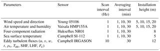

Figure 1(a) Yongxing Island air–sea flux tower (YXASFT). (b) Instrumentation and data acquisition system mounted on the YXASFT. (c) Pictures of some sensors on the YXASFT. (d) Google satellite image of Yongxing Island. The red triangle indicates the location of the YXASFT. (e) Map of the northern SCS. The black star indicates the location of Yongxing Island.
Accurate calculations of air–sea fluxes play a crucial role in driving marine and atmospheric circulation models, understanding atmosphere–ocean interactions, and evaluating and assessing numerical weather forecast models (Sun et al., 2003). Currently available air–sea flux datasets (including satellite remote sensing inversion data and reanalysis data) are quite uncertain, as they are mainly derived from inaccurate flux modeling algorithms, and uncertainties in the turbulent exchange coefficient were also involved in the fluxes calculations (Zeng et al., 1998; Josey, 2001; Smith et al., 2001). In turn, these intrinsic uncertainties limit the ability to assess numerical models based on reanalysis flux datasets (Yu et al., 2006).
The South China Sea (SCS) is mainly controlled by various monsoon systems. It is connected with the western Pacific Ocean and the Indian Ocean through marine and atmospheric processes, and thus, the SCS exhibits potential influences on global climate change as well as regional climate regimes (Wang et al., 2006; Shi et al., 2015). Air–sea interactions in the SCS induce many marine meteorological hazards and greatly affect the transfer of heat and water vapor in regions throughout south China and Southeast Asia (Yang et al., 2015). Acquiring long-term observations of air–sea fluxes in the SCS can therefore help us to better understand the characteristics and evolutionary behavior of air–sea interactions in the SCS, optimize the parameterization schemes in atmospheric models, and improve long-term weather forecasts and extreme hazardous weather alerts.
To achieve the abovementioned scientific goals, a mesoscale observation network in the Xisha sea area in the northern SCS was initiated in 2008 (Yang et al., 2015) with the primary ambition of researching air–sea interactions. At present, the observation network includes a surface mooring buoy array, a system of shore-based wave–tide gauges, an automatic weather station, a shore-based boundary layer air–sea flux tower and a submerged mooring buoy array. A large dataset comprising of in situ observational data was obtained to serve as baseline reference data to quantify the uncertainties within regional model flux products for the SCS.
Many in situ observations and model analysis comparisons have been studied in different oceans around the world, including the Arabian Sea (Weller et al., 1998; Swain et al., 2009), the tropical Pacific Ocean (Weller and Anderson, 1996; Wang and McPhaden, 2001), the northeast Atlantic Ocean (Sun et al., 2003; Yu et al., 2004), the Indian Ocean (Goswami, 2003) and the SCS (Zeng et al., 2009; Wang et al., 2013). Unfortunately, due to limited field observations of flux-related variables, detailed evaluation studies in the SCS are scarce.
In this study, turbulent SHF and LHF variations as well as numerous bulk variables, including the air temperature (Ta), sea surface temperature (Ts), air humidity (Qa) and wind speed (U), from the Woods Hole Oceanographic Institution (WHOI) Objectively Analyzed Air–Sea Fluxes (OAFlux) project are compared with the Yongxing air–sea flux tower (YXASFT) measurements in the northern SCS. This investigation spans a full year from 1 February 2016 to 31 January 2017. Seasonal comparisons of the bulk variables and heat fluxes are described in Sect. 3. An overview of the instrumentation on the Yongxing air–sea flux tower in addition to the data and methodology employed in this paper are introduced in Sect. 2. Finally, the summary and conclusions are provided in Sect. 4.
2.1 The Yongxing air–sea flux tower (YXASFT)
The 20 m tall YXASFT (Fig. 1a), which was specially designed for the observation of air–sea boundary layer fluxes, is located approximately 100 m off the northeastern coastline of Yongxing Island (16.84∘ N, 112.33∘ E; Fig. 1d and e). A gradient meteorological system (GMS) and an eddy covariance flux (ECF) system were mounted on the tower (Fig. 1b). A CR3000 data logger manufactured by Campbell Scientific Company, USA, is used for data sampling, preprocessing, storage and transmission. The real-time observation data from the YXASFT are open for access at the website http://mabl.scsio.ac.cn:8040 (login: CSL-CER and password: ruhuna, last access: 6 November 2018). A data sharing agreement must be signed by the user before being authorized to download the data.
Table 2Information regarding the adopted in situ and reanalysis data.*
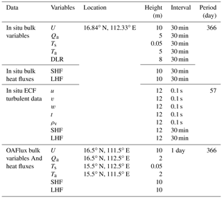
u: wind speed along the sonic x axis, v: wind speed along the sonic y axis, w: wind speed along the sonic z axis, t: sonic temperature, ρv: water vapor density. The height of the bulk fluxes derived via COARE3.0 for both in situ data and OAFlux are considered at 10 m.
The sensor wiring and data acquisition diagram for the YXASFT is shown in Fig. 2. The observational variables within the GMS include U, the wind direction (Wd), Ta, Qa, the air pressure (Pa), the net radiation (Rn) and Ts. Each parameter is sampled once every second, and 1, 10 and 30 min averages are recorded and transmitted to the data center in real-time. The ECF system can collect high-frequency turbulent data with a 10 Hz sampling frequency. Successive 30 min fully corrected fluxes of the momentum (Tau), SHF, LHF and CO2 (Fc) can be calculated using the online program EasyFlux (Campbell Scientific, Inc.). The sensors in the YXASFT and their respective measurement specifications are listed in Table 1. All of the sensors (Fig. 1c) have been checked via pre- and post-installment calibrations by the National Center of Ocean Standards and Metrology.
2.2 Data
The data employed in this study originate from two sources: the in situ observations obtained by YXASFT and the reanalysis datasets derived from the OAFlux project. Table 2 shows various information, including the variable height, time period, interval and location, regarding the data adopted in this study.
2.2.1 In situ data
High-frequency turbulent data (u, v, w, t, ρv) were collected by the ECF system installed at a height of 12 m from 1 February 2016 to 29 March 2016. Direct measurements of turbulent data were further used to calculate the fluxes using the eddy covariance (EC) method in a specified time period (30 or 60 min). Meanwhile, direct measurements of turbulent fluxes using the ECF system were used only to verify the applicability of version 3.0 of the Coupled Ocean–Atmosphere Response Experiment (COARE3.0) over the SCS.
The selected 30 min averages of the bulk variables (U measured at a height of 10 m and Ta, Qa and Ts measured at a height of 5 m) used for the bulk flux calculations range from 1 February 2016 to 31 January 2017. Note that Ts was measured using an SI-112 infrared radiation thermometer manufactured by Campbell Scientific Company, USA, installed at a height of 5 m, and therefore, we consider Ts representative of the sea surface temperature at a depth of 0.05 m. The value of Qa was derived using Eq. (1) as described in COARE3.0 using Ta, the relative humidity (Rh) and the air pressure (Pa). Furthermore, this paper also adopts SHF and LHF averages within 30 min intervals derived via COARE3.0 using the input observed bulk variables. The heights of Ta and Qa in the OAFlux dataset are both 2 m, while the measurement heights for these two parameters on the YXASFT are both 5 m. Thus, prior to conducting a comparison, we corrected the corresponding heights of the in situ data to correspond to the heights in the OAFlux dataset using COARE3.0. In addition, downward longwave radiation (DLR) data measured using an NR01 net radiometer manufactured by Hukseflux were used in this paper as an indirect variable to infer the cloud cover in the sky.
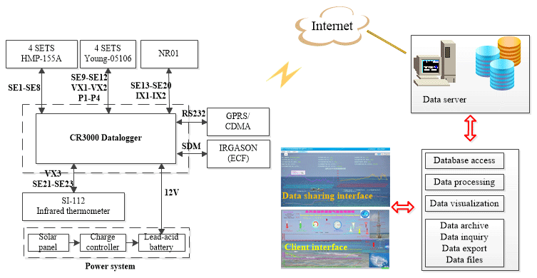
Figure 2Diagram of the real-time data acquisition system and the sensor wiring scheme on the YXASFT (SE: single-ended channel, VX: voltage excitation channel, P: pulse-input channel, IX: current excitation channel, SDM: SDM channel, GPRS: General Packet Radio Service, CDMA: code-division multiple access; Campbell Scientific, Inc., 2018).
2.2.2 Reanalysis data
In this paper, the OAFlux reanalysis data were selected for two reasons. First, a previous study showed that the OAFlux dataset is the most preferable among five different products (i.e., ERA-1, NCEPS, JRA55, TropFlux and OAFlux) with regard to LHF data over the SCS (Wang et al., 2017; Zhang et al., 2018). Second, OAFlux represents the most recently updated data product (as of July 2017) accessible for the study period. OAFlux is an ongoing global flux product compiled by WHOI with a spatial resolution of 1∘ × 1∘. OAFlux utilizes an integrated analysis method to combine satellite data with modeling and reanalysis data, and it employs COARE3.0 to calculate heat fluxes (Yu et al., 2008). In this study, the daily mean OAFlux datasets include U, Qa, Ts, Ta, LHF and SHF, and YXASFT observations during the same time period were used for a comparison.
2.3 Methods
2.3.1 Bulk algorithm
The bulk algorithm utilized in this study is based on the Monin–Obukhov similarity theory, which is widely considered to be an advanced bulk algorithm (Fairall et al., 1996). To keep consistent with the bulk method of calculating flux in OAFlux, the COARE3.0 was used to calculate the heat fluxes using the in situ observation bulk parameters in this paper. Compared to COARE2.5, the updated COARE3.0 has some noted improvements as follows. First, the range of wind speed validity is now extended to 0–20 m s−1 after modifying roughness representation. Second, the COARE 3.0 is shown to be accurate within 5 % for wind speeds of 0–10 m s−1 and 10 % for wind speeds between 10 and 20 m s−1 (Fairall et al., 2003). In this method, the calculation equations for the SHF and LHF can be written as follows:
where ρa represents the air density, Cp represents the latent heat of evaporation, Cp represents the constant-pressure specific heat, U represents the sea surface wind speed (measured at a height of 10 m in this study), Ce and Ch correspond to the turbulence exchange coefficients for the latent heat and sensible heat, respectively, Qs and Qa correspond to the air saturation specific humidity at the sea surface and the air specific humidity near the sea surface, respectively, and Ts and Ta correspond to the sea surface skin temperature and the air temperature near the sea surface, respectively. In Eqs. (2) and (3), only U, Ts, Ta and Qa are independent measurement variables, while the remainder of the variables must be calculated based on the four independent variables.
2.3.2 Eddy covariance method
The EC method is one of the most direct ways to measure and calculate turbulent fluxes (Crawford et al., 1993). The Reynolds decomposition is utilized to break raw data down into their means and deviations. Furthermore, the values of SHF and LHF can be calculated as the covariance between w and scalar values (t, ρv) using the following formulas, respectively:
where ρ is the dry air density, Cp is the specific heat of dry air at a constant pressure (where 1004.67 Jkg−1 K−1 is used in the calculation) and λ is the latent heat ratio of water vapor evaporation. The overbar represents the Reynolds ensemble average, and the prime symbol denotes the instantaneous deviation from the ensemble average.
2.3.3 Data processing
To match the timescale of the OAFlux daily data, we derived the daily means of the YXASFT-observed bulk variables and heat fluxes by averaging all of the 30 min datasets from each day. In addition, we used bilinearly interpolated OAFlux values (inversely weighted by the distance) from the surrounding four grid points (16.5∘ N, 111.5∘ E; 16.5∘ N, 112.5∘ E; 15.5∘ N, 112.5∘ E; 15.5∘ N, 111.5∘ E) to represent the corresponding OAFlux value at the YXASFT observation site.
The comparison between the YXASFT and OAFlux datasets (described in Sects. 3 and 4) was quantitatively analyzed by using the mean bias (Bias, defined in Eq. 6), root mean square error (RMSE, defined in Eq. 7), coefficient of determination (R2) and linear regressions.
where x and y denote the OAFlux values and YXASFT observations, respectively.
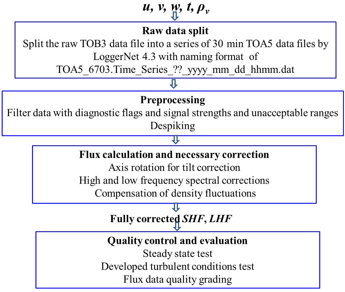

Figure 4Daily means of the LHF and SHF time series (a) and scatter plots (b) of COARE3.0 versus ECF (from 1 to 29 March 2016). The R2 values, linear regressions and numbers of matched pairs (N) are given in the bottom panels. The solid red line refers to the linear regression of the matched pairs. The solid green line y=x indicates a 1:1 correspondence.
3.1 Validation of COARE3.0 using direct ECF measurements
The heat fluxes from both YXASFT and OAFlux used for the comparison herein were derived from COARE3.0. However, the COARE algorithm was originally developed for the Tropical Ocean Global Atmosphere-COARE (TOGA-COARE) experiment in tropical oceans (Fairall et al., 1996), while the reliability of COARE3.0 was verified by (Brunke et al., 2003) using 12 ship cruises over tropical and mid-latitude oceans (between 5∘ S and 60∘ N). The adaptability of OAFlux in the SCS must be verified due to its unique geographical location (i.e., it is the largest marginal sea in the northwestern Pacific Ocean) and its monsoon climate system. In this study, the EC fluxes directly measured by the IRGASON ECF system were used to validate the performance of COARE3.0 in the SCS. The EC method is mathematically complex, significant care is required to set up different processing steps for different sites, measurements and study purposes. In this paper, the EC program running on CR3000 was based on the processing steps shown in Fig. 3. The daily LHF time series in COARE3.0 are basically consistent with those in ECF (Fig. 4a), with an R2 value of 0.78 (Fig. 4c). COARE3.0 underestimates the LHF with a mean bias of 18.55 w m−2. A larger difference in the LHF measurement occurs when relatively larger LHF values are observed (e.g., 7 and 25 February 2016), which can be readily observed in Fig. 4a. The precipitation on these days is the most likely explanation for the overestimation in the LHF by the ECF system (Mauder et al., 2006; Zhang et al., 2016). Although the YXASFT possesses a lack of field precipitation observations, we can speculate that precipitation may have occurred on 7 February 2016 based on a 1.8 ∘C drop in the air temperature and an increase of 13 % in the relative humidity within the daily mean. In addition, we spot similar trends on 25 February 2016. In contrast, the SHF data pair is far from agreement, with an R2 value of 0.03 (Fig. 4d). The large variation in the SHF observed using the ECF is not detected within the COARE3.0-derived time series (Fig. 4b). Direct heat flux measurements with a 60 day interval obtained using the ECF system show that SHF (with a mean of 23.5 w m−2) is significantly smaller than LHF (with a mean of 93.3 w m−2). A small SHF magnitude may amplify variations in the time series and reduce the R2 values in scatter plots under the same deviation values. In this comparison, we were more concerned about the magnitude of correlation in the LHF data. Thus, COARE3.0 was considered to be receptive and was used as an appropriate bulk flux algorithm over the SCS.
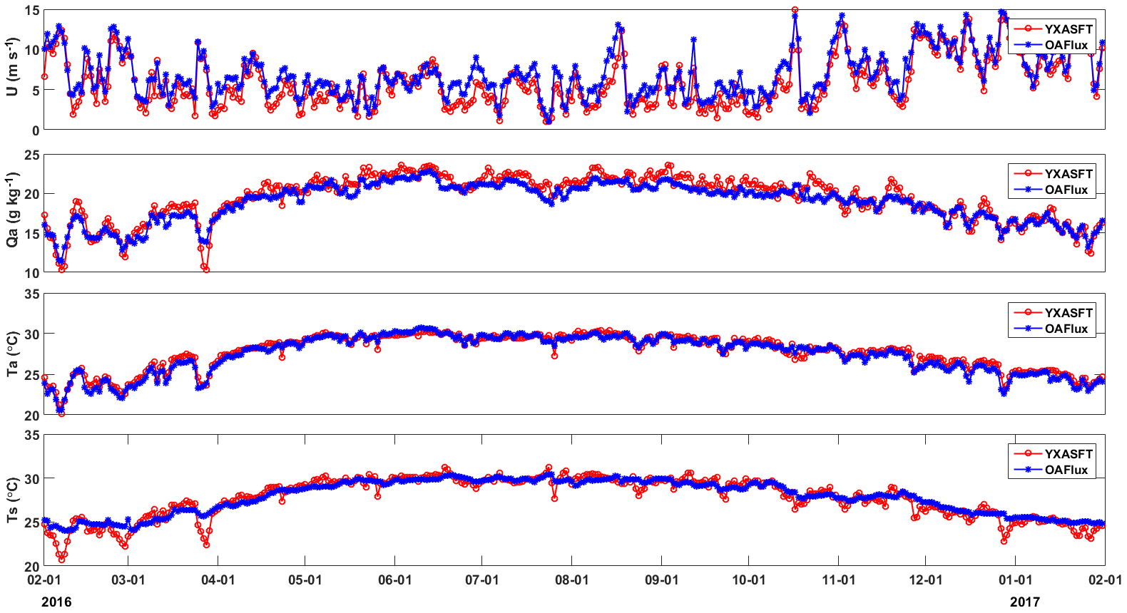
Figure 5Daily mean time-series plots of the YXASFT-observed (red solid lines) and OAFlux-analyzed (blue solid lines) U, Qa, Ta and Ts values over the study period (1 February 2016–31 January 2017).

Figure 6Daily mean time-series plots of the YXASFT-observed (red solid lines) and OAFlux-analyzed (blue solid lines) SHF and LHF over the study period (1 February 2016–31 January 2017).
3.2 Evaluation of the OAFlux datasets
OAFlux is a flux product based on a composite algorithm that improves the calculation accuracies of flux-related variables by using a weighting method for target analysis. However, this method could lead to a timescale mismatch if the data variables have different data sources (Fairall et al., 2010). It is therefore necessary to evaluate the OAFlux dataset to assess its applicability in the SCS before further application.
3.2.1 Time series of the YXASFT observations and OAFlux reanalysis data
Time series of the bulk variables and heat fluxes are given in Figs. 5 and 6, respectively. As shown in Fig. 6, there is an obvious overestimation in both SHF and LHF in OAFlux compared with the YXASFT observations, and this overestimation demonstrates an evident seasonal variation. The time series of LHF from the YXASFT observations and OAFlux data show essentially consistent variation trends and agree with one another better during the spring (February to March) and winter (December to January) than during the summer and autumn (April to November) (Fig. 6b). The SHF variation trend appears to be opposite to that of LHF, since the deviations during the winter and spring are clearly larger than those during the summer and autumn (Fig. 6a). For the bulk variables in Fig. 5, the OAFlux data maintained a higher consistency with the YXASFT observations with regard to the overall variation trend. Furthermore, U and Qa seemed to match better during the winter and spring periods, while an overestimation (underestimation) in U (Qa) is more evident during the summer and autumn periods (Fig. 5a and b). Some abrupt drops (i.e., variations of 3 to 5 days) in the YXASFT Ts observations were obviously not captured by OAFlux (Fig. 5d). In the next section, we divide the annual study period into three periods, namely, spring (1 February 2016–31 March 2016), summer–autumn (1 April 2016–31 November 2016) and winter (1 December 2016–31 January 2017), to conduct a detailed comparison of their seasonal variations.
Table 3Quantitative statistical summary based on comparisons between daily YXASFT measurements and daily OAFlux products in the spring, summer–autumn and winter periods.
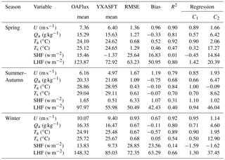
OAFlux YXASFT +C2.
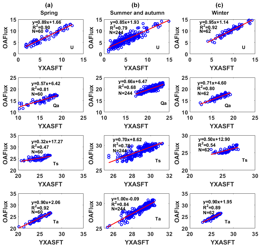
Figure 7Scatter plots of the YXASFT and OAFlux wind speeds at 10 m (U), air specific humidity at 2 m (Qa), and sea surface temperatures (Ts) and air temperatures at 2 m (Ta) during the spring (a), summer–autumn (b) and winter (c) periods. The units for U, Qa, Ts and Ta are m s−1, g kg−1, ∘C and ∘C, respectively. The linear regression equation, coefficient of determination (R2) and number of matched pairs (N) are given in each panel. The solid red line refers to the linear regression of the matched pairs.
3.2.2 Comparison of the bulk variables
The heat fluxes from both OAFlux and YXASFT were derived using COARE3.0. Thus, we can further analyze the origin of the seasonal deviations in the heat fluxes by conducting seasonal comparisons of the bulk variables. The scatter plots of U, Qa, Ts and Ta constructed using the YXASFT and OAFlux data for the three separate periods are shown in Fig. 7, and a quantitative statistical summary for each variable is listed in Table 3.
U. The spring, summer–autumn, and winter periods on Yongxing Island represent the monsoon transition, southwest monsoon and northeast monsoon periods, respectively. Previous studies indicated that the northeast monsoon in the northern SCS is much stronger than the southwest monsoon (Yan et al., 2005). In this study, the observed mean wind speeds during the three periods were 6.40, 4.97 and 9.40 m s−1, respectively. It can be seen from Fig. 7 (first row) that the R2 values of U between the OAFlux and YXASFT data during the three periods are 0.90, 0.79 and 0.92, respectively. OAFlux overestimates the values of U in the spring, summer–autumn, and winter periods with mean biases of 0.96 (15 % of the YXASFT-observed mean value), 1.19 (24 %) and 0.67 m s−1 (7 %), respectively.
Qa. The southwest monsoon is often accompanied by a high amount of water vapor and cloudy skies (Chen et al., 2012). Therefore, the Qa value during the summer–autumn period was the highest throughout the year, with an observed mean of 21.08 g kg−1. The R2 values of Qa between the OAFlux and YXASFT data during the three periods are 0.81, 0.68 and 0.80, respectively (Fig. 7, second row). In contrast to U, OAFlux exhibits an overall underestimation of Qa in the spring, summer–autumn, and winter periods with dry biases of 0.33 (2 %), 0.75 (4 %) and 0.11 g kg−1 (1 %), respectively.
Ta. The OAFlux Ta values are highly consistent with the YXASFT observations, with R2 values of 0.92, 0.84 and 0.89 in the spring, summer–autumn, and winter periods, respectively (Fig. 7, fourth row). As shown in Fig. 5c, both the seasonal trends and day-to-day variations are effectively captured in the OAFlux data. The OAFlux reanalyzed Ta data have a warmer bias of 0.52 ∘C (2 %) in the spring and colder biases of 0.10 (0.3 %) and 0.57 ∘C (2 %) in the summer–autumn and winter periods, respectively. Consequently, the OAFlux-estimated Ta can be considered as the most reliable variable in this study.
Ts. The OAFlux-estimated Ts only captures the seasonal trend, and the estimates exclude some special synoptic signals, such as abrupt drops during cold air temperatures and typhoons or gradual temperature increases induced by the passage of a warm eddy. The R2 values of Ts between the OAFlux and YXASFT data are relatively small when compared with those of U, Qa and Ta, suggesting that the reliability of the OAFlux-analyzed Ts is generally low. In contrast to U and Qa, the OAFlux Ts performance was better in the summer–autumn period (R2=0.70) than in the spring (R2=0.47) and winter (R2=0.54) periods, as shown in Fig. 7 (third row).
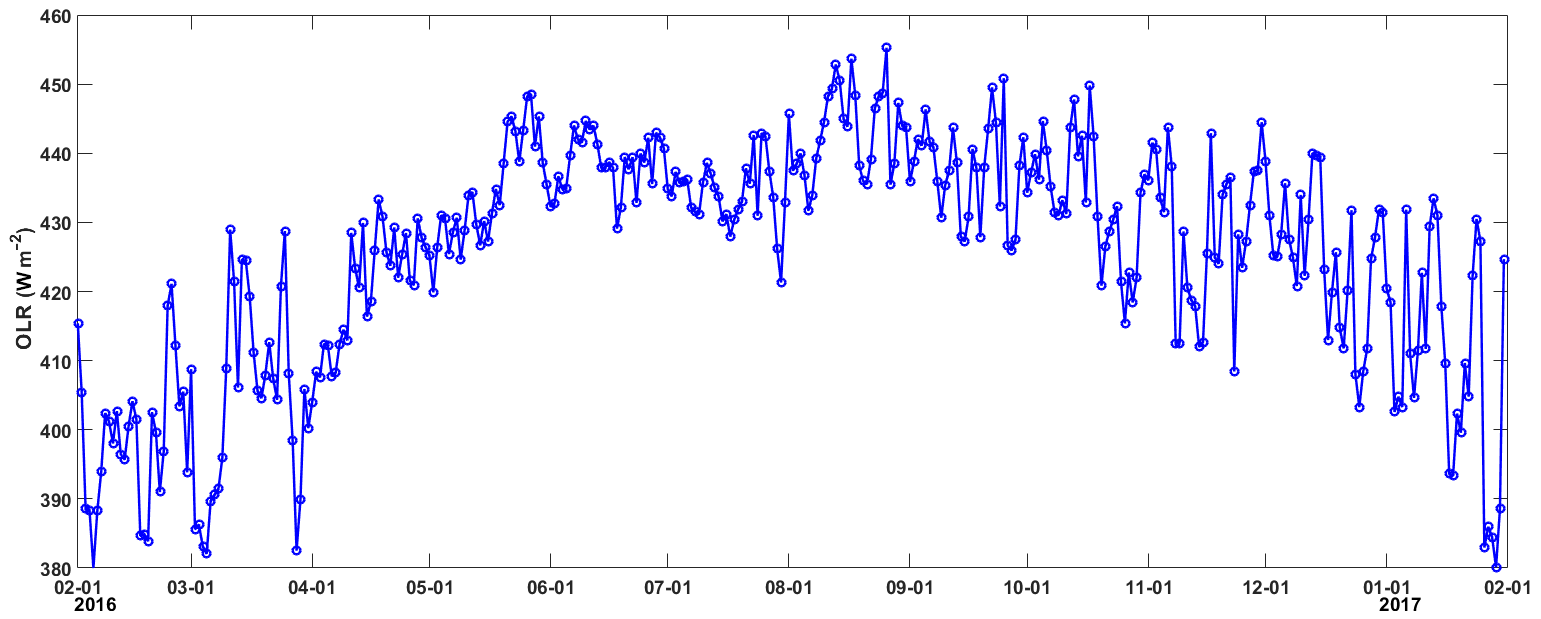
Figure 8Daily mean time-series plots of the YXASFT observed downward long radiation (DLR) over the study period (1 February 2016–31 January 2017).
In summary, the seasonal performances of the OAFlux-estimated U and Qa seem to be highly correlated with the monsoon system in the SCS. This manifests as a better performance of the OAFlux-estimated U (Qa) during the spring and winter periods, characterized by a stronger (drier) northeast monsoon than during the summer–autumn period, characterized by a relatively weaker (wetter) southwest monsoon. The significant difference between the Ts estimates may stem largely from the fact that the OAFlux Ts estimates are retrieved using a advanced very-high-resolution radiometer (AVHRR), which is easily affected by the presence of clouds. Therefore, the available OAFlux Ts estimates were dramatically reduced during the abovementioned special synoptic processes. With the onset of the southwest monsoon, the average total cloud cover, low cloud cover and precipitation all increase throughout the SCS (Yan et al., 2003), and the Ts retrieved via the AVHRR should correspondingly exhibit a lower quality. However, this trend is not observed in the result of this paper. We further utilized in situ observations of the DLR to infer the sky cloud cover. There is an evidently greater fluctuation in the DLR during the winter and spring periods than in the summer–autumn period, indicating that the winter and spring seasons possess greater probabilities of cloudy days (Fig. 8). This interesting phenomenon may be caused by the fact that the intensity of the summer monsoon in 2016 was weaker than those in preceding years; this hypothesis will be further explored hereafter.
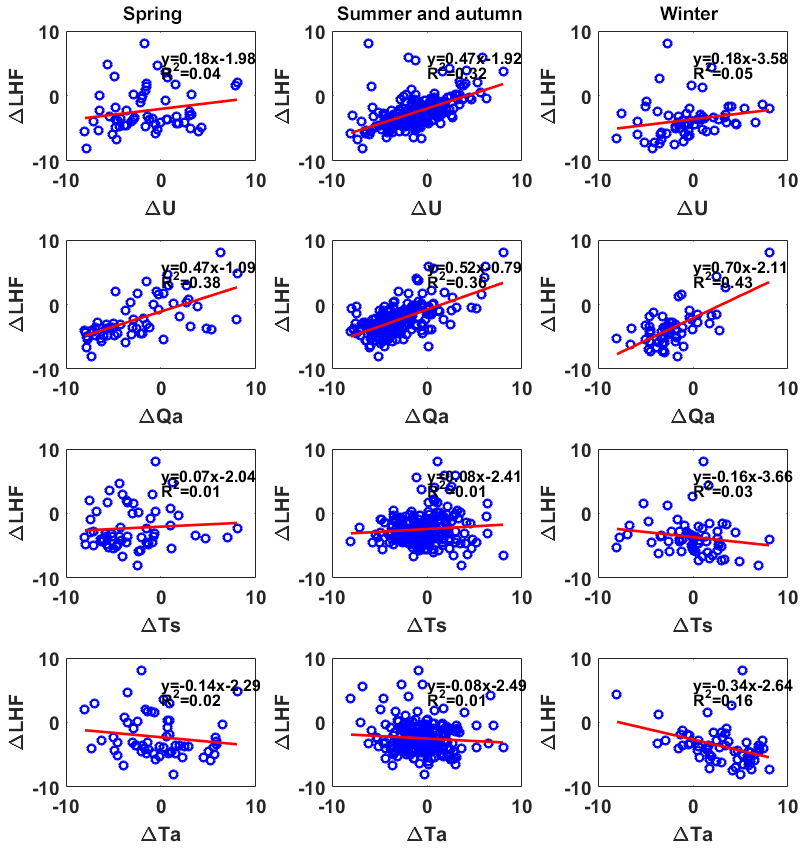
Figure 10Scatter plots for the biases of U (ΔU), Qa (ΔQa), Ts (ΔTs), and Ta (ΔTa) with respect to the biases of LHF (ΔLHF). All of the data are normalized to the range of −10 to 10 in this paper. The linear regression equation and coefficient of determination (R2) are given in each panel. The solid red line refers to the linear regression of the matched pairs.
3.2.3 Comparison of heat fluxes
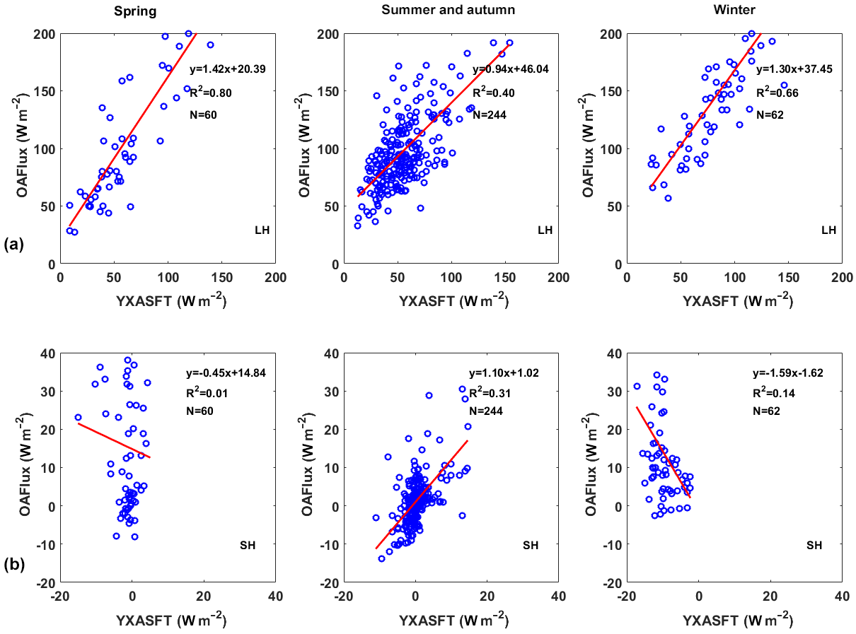
The scatter plots of the LHF and SHF estimates obtained from the YXASFT and from OAFlux during the three periods are shown in Fig. 9, and a quantitative statistical summary of each variable is also listed in Table 3. Note that an upward (downward) heat flux is positive (negative) in this paper, and a positive (negative) value represents the loss (gain) of ocean heat to (from) the atmosphere.
LHF. Compared with the YXASFT observations, the OAFlux-estimated LHF is overestimated by a mean bias of 50.95 (70 %) in the spring, 42.43 (76 %) in the summer–autumn and 63.29 w m−2 (74 %) in the winter. The R2 values are 0.80 in the spring, 0.66 in the winter and 0.40 in the summer–autumn (Fig. 9, first row). This is also consistent with the R2 values for U and Qa, which are the two key input factors in the LHF calculations.
SHF. Large SHF variations during the spring and winter are not evident in the YXASFT-derived SHF time series (Fig. 5e). Compared to LHF, the OAFlux-estimated SHF has the smallest R2 values for all three individual periods, as shown in Table 3 for the spring (0.01), summer–autumn (0.31) and winter (0.14). In comparison, the OAFlux-estimated SHF is more reliable during the summer–autumn, with a mean bias of 1.07 w m−2 than in the spring (16.83 w m−2), or winter (23.56 w m−2).
Overall, we can infer that the OAFlux-estimated LHF product is more reliable during the spring and winter periods than during the summer–autumn period, which is consistent with the key input variables U and Qa, and that the product is further affected by the monsoon system in the SCS. Meanwhile, the SHF estimates exhibit opposite characteristics relative to those of LHF, as the OAFlux SHF product is more credible during the summer–autumn than during the spring and winter periods, which is consistent with the seasonal OAFlux Ts performance and is highly correlated with the cloud cover.
3.3 Possible effects of bulk variables on the biases in the SHF and LHF
The values of SHF and LHF were calculated using Eqs. (2) and (3). Thus, possible biases in the LHF and SHF results are mainly associated with the input bulk variables and the parameterization of the turbulent exchange coefficients in the equations. In this paper, the parameterization scheme is not discussed due to limited space. The relationships among the OAFlux LHF bias with U, Qa and Ts were studied extensively by a previous study through years of moored buoy data, automatic weather station (AWS) data and cruise data over different regions in the SCS; it was found that the biases in Qa dominated the LHF biases, followed by the biases in U (Wang et al., 2017). To determine whether similar conclusions exist in this study and to quantify the relationships among the heat flux biases and the bulk variable biases, we constructed scatter plots of the biases in LHF (Fig. 10) and SHF (Fig. 11) against the biases in U, Qa, Ts and Ta. All of the biased data were normalized first to understand their relative importance.
ΔLHF. The biases in Qa are the most dominant factor in determining the biases in LHF during the spring, with relatively high R2 values of 0.38 compared with the other biased bulk variables (Fig. 10, first column). Both of the Qa and U biases are responsible for controlling the biases in LHF during the summer–autumn period with R2 values of 0.36 and 0.32, respectively (Fig. 10, second column). Both of the Qa and Ta biases are the dominant factors in determining the bias in LHF during the winter period, with R2 values of 0.43 and 0.16, respectively (Fig. 9, third column). The biases in Ts are negligible control factors on the biases in LHF since their R2 values are all relatively small during the three periods compared with those of Qa (Fig. 9, third and fourth rows). In general, the result revealed that the Qa is the most dominant factor controlling the biases in LHF throughout the year, which is similar to those reported in previous studies (Wang et al., 2013, 2017). Additionally, these dominant factors that cause the seasonal biases in LHF are new findings in this article.
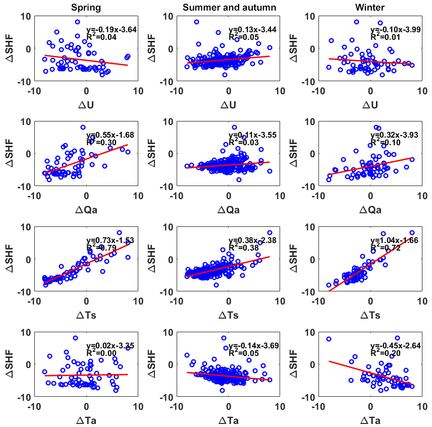
ΔSHF. During the observational period, the biases in Ts were the key factor dominating the biases in SHF. The effects of Ts biases on the biased SHF during the spring (R2=0.79) and winter (R2=0.72) periods were much larger than that during the summer–autumn period (R2=0.38), which is also consistent with the fact that OAFlux estimates Ts better in the summer–autumn than in the spring and winter (Fig. 7, third row). From Eq. (2), SHF is largely determined by Ts–Ta, as shown in Fig. 6. OAFlux is unable (able) to capture the variations in Ts (Ta) during the spring and winter, thereby causing large fluctuations in Ts–Ta and further leading to large variabilities in the OAFlux SHF time series.
Successive air–sea heat flux-related observational data were acquired over the course of a year (1 February 2016–31 January 2017) at the YXASFT on Yongxing Island. In this paper, we first used direct heat flux measurements from a high-frequency (10 Hz) ECF system to validate the reliability of the COARE3.0 bulk algorithm in the SCS. Then, seasonal comparisons were conducted for the daily mean surface bulk variables and heat fluxes between the WHOI OAFlux products and YXASFT observations. Finally, the effects of biased bulk variables on the biases in the heat fluxes were presented to determine the possible sources of the biases in LHF and SHF. The conclusions are summarized as follows.
The magnitude of the mean of the directly measured SHF is small compared with that of LHF and can even be ignored in air–sea heat flux interactions during the ECF measurement period. Therefore, we were more concerned with the LHF estimation differences between COARE3.0 and the ECF system in this validation. The daily mean LHF from COARE3.0 was basically consistent with the ECF measurements with a high R2 and an acceptable bias. Furthermore, if possible precipitation periods were excluded, the consistency between the COARE3.0 and ECF LHF data were better. Thus, the COARE3.0 bulk algorithm was considered to be reliable in this study.
Comparisons of the bulk variables revealed that the reliabilities of the OAFlux datasets diminished in the order of Ta, U, Qa and Ts based on a combination of R2 values and biases. The performances of the OAFlux-estimated U and Qa seem to be highly correlated with the monsoon system in the SCS; OAFlux provides a better estimation of U (Qa) in the spring and winter, characterized by a stronger (drier) northeast monsoon than in the summer–autumn characterized by a relatively weaker (wetter) southwest monsoon. Similar to a previous study, this study also indicated that Ts is the least reliable OAFlux product (Sun et al., 2003). The Ts signals during special synoptic process were poorly captured by OAFlux due to the presence of clouds, which affect the recorded AVHRR data. The performance of the OAFlux-estimated Ts is better during the summer–autumn than in the winter or spring due to a reduced cloud cover during the summer monsoon period, which could be attributable to the fact that the summer monsoon in 2016 was weaker than those in preceding years. With respect to a comparison of the heat fluxes, OAFlux considerably overestimates LHF with ocean heat loss biases of 50.95 w m−2 (70 %) in the spring, 42.43 w m−2 (76 %) in the summer–autumn and 63.29 w m−2 (74 %) in the winter. Consistent with the key input variables U and Qa, the OAFlux LHF performance is better during the spring and winter than in the summer–autumn, which is further associated with the monsoon climate in the SCS. The seasonal SHF reliability is coincident with that of Ts, as the least reliable Ts estimates lead to the most unreliable SHF estimates, with enormous overestimations throughout the year. An analysis of the possible sources of biases in the heat fluxes show that biases in Qa are the most dominant factor in determining the biases in LHF during the spring and winter. Meanwhile, both of the biases in Qa and U are responsible for controlling the biases in LHF during the summer–autumn period. Biases in Ts are responsible for controlling the biases in SHF, and the effects of biases in Ts on the biases in SHF during the spring and winter are much greater than that in the summer–autumn period.
In summary, both Ts and SHF in OAFlux should be utilized with considerable caution in further research. Additionally, U, Qa and LHF should be used with proper consideration due to their seasonal reliability variations. Researchers should feel more at ease using these data during the northeast monsoon than in the southwest monsoon. The performance of the OAFlux-estimated Ta seems to change little with the seasons and is highly consistent with the YXASFT observations throughout the year. Improving the observation capability of the AVHRR sensor under cloudy conditions is necessary for improving the accuracy of Ts estimates and the reliability of calculating SHF. Larger quantities of in situ bulk variable observations and direct turbulent heat flux measurements as well as improvements in the parameterization of variables in different regions of the SCS are also essential for improving the reliability of OAFlux datasets in the SCS.
According to the project management requirements, the in situ data observed from YXASFT were not publicly accessible. Any interested readers can access these data by email to the first author or the correspondence author, and we will send the data file to you directly by email.
The supplement related to this article is available online at: https://doi.org/10.5194/amt-11-6091-2018-supplement.
FZ designed the experiments and RS, JC and YH carried them out. FZ and RZ wrote the Matlab program and performed the data processing and analysis. QX and DW assisted with useful discussions and data collection. FZ and QX prepared the manuscript with contributions from all co-authors.
The authors declare that they have no conflict of interest.
This study was funded by the Key
Research Program of Frontier Sciences, Chinese Academy of Sciences (CAS)
(QYZDJ-SSW-DQC022); the National Natural Science Foundation of China
(41706102); the Chinese Academy of Sciences (CAS) Key Technology Talent
Program of 2016; the Station Network Construction Project, Xisha Marine
Observatory of the CAS (KZCX2-YW-Y202). Rongwang Zhang was also supported by
the National Key R&D Program of China (grant no. 2017YFA0603200). The
YXASFT data were provided by the Xisha Deep Sea Marine Environment
Observation Station, South China Sea Institute of Oceanology, CAS. All of
the in situ data adopted in this study can be obtained by contacting the
first author, Fenghua Zhou (zhoufh@scsio.ac.cn). The authors would like to
express their gratitude for the reanalysis data products comprising global
ocean heat flux and evaporation data provided by the WHOI OAFlux project
(http://oaflux.whoi.edu, last access: 6 November 2018) funded by the NOAA Climate Observations and
Monitoring (COM) program. The source code for the COARE 3.0 algorithm is
freely available at http://coaps.fsu.edu/COARE/flux_algor/ (last access: 6 November 2018).
The first author would like to thank the engineers from Campbell Scientific
Company, USA, for their help with the observation system integration and
data acquisition on the YXASFT. Finally, the authors thank the anonymous
reviewers for their valuable comments and suggestions that improved the
quality of this paper.
Edited by: Marcos Portabella
Reviewed by: two anonymous referees
Brunke, M. A., Fairall, C. W., Zeng, X., Eymard, L., and Curry, J. A.: Which bulk aerodynamic algorithms are least problematic in computing ocean surface turbulent fluxes?, J. Climate, 16, 619–635, https://doi.org/10.1175/1520-0442(2003)016<0619:WBAAAL>2.0.CO;2, 2003.
Campbell Scientific, Inc.: CR3000 Micrologger User's Manual, available at: https://s.campbellsci.com/documents/us/manuals/cr3000.pdf, last access: 21 March 2018.
Chelton, D. and Xie, S.-P.: Coupled Ocean-atmosphere interaction at oceanic mesoscales, Oceanography, 23, 52–69, https://doi.org/10.5670/oceanog.2010.05, 2010.
Chen, J., Zuo, T., and Wang, H.: Variation of latent heat flux over the Bengal Bay-South China Sea area and its relationship with South China Sea summer monsoon onset, Int. Geosci. Remote Se., Munich, Germany, 22–27 July 2012, 856–859, 2012.
Crawford, T. L., McMillen, R. T., Meyers, T. P., and Hicks, B. B.: Spatial and temporal variability of heat, water vapor, carbon dioxide, and momentum air-sea exchange in a coastal environment, J. Geophys. Res., 98, 12869–12880, https://doi.org/10.1029/93jd00628, 1993.
Fairall, C. W., Bradley, E. F., Rogers, D. P., Edson, J. B., and Young, G. S.: Bulk parameterization of air-sea fluxes for tropical ocean-global atmosphere coupled-ocean atmosphere response experiment, J. Geophys. Res., 101, 3747–3764, https://doi.org/10.1029/95jc03205, 1996.
Fairall, C. W., Barnier, B., Berry, D. I., Bourassa, M. A., Bradley, E. F., Clayson, C. A., de Leeuw, G., Drennan, W. M., Gille, S. T., Gulev, S. K., Kent, E. C., McGillis, W. R., Quartly, G. D., Ryabinin, V., Smith, S. R., Weller, R. A., Yelland, M. J., and Zhang, H.-M.: Observations to quantify air-sea fluxes and their role in climate variability and predictability, in: Proceedings of OceanObs'09: Sustained Ocean Observations and Information for Society, edited by: Hall, J., Harrison, D. E., and Stammer, D., European Space Agency, Noordwijk, the Netherlands, 299–313, 2010.
Frenger, I., Gruber, N., Knutti, R., and Münnich, M.: Imprint of Southern Ocean eddies on winds, clouds and rainfall, Nat. Geosci., 6, 608–612, https://doi.org/10.1038/ngeo1863, 2013.
Goswami, B. N.: A note on the deficiency of NCEP/NCAR reanalysis surface winds over the equatorial Indian Ocean, J. Geophys. Res., 108, 3124, https://doi.org/10.1029/2002jc001497, 2003.
Hogg, A. M. C., Dewar, W. K., Berloff, P., Kravtsov, S., and Hutchinson, D. K.: The effects of mesoscale ocean–atmosphere coupling on the large-scale ocean circulation, J. Climate, 22, 4066–4082, https://doi.org/10.1175/2009JCLI2629.1, 2009.
Josey, S. A.: A Comparison of ECMWF, NCEP–NCAR, and SOC Surface heat fluxes with moored buoy measurements in the subduction region of the Northeast Atlantic, J. Climate, 14, 1780–1789, https://doi.org/10.1175/1520-0442(2001)014<1780:acoenn>2.0.co;2, 2001.
Mauder, M., Liebethal, C., Göckede, M., Leps, J.-P., Beyrich, F., and Foken, T.: Processing and quality control of flux data during LITFASS-2003, Bound.-Lay. Meteorol., 121, 67–88, https://doi.org/10.1007/s10546-006-9094-0, 2006.
Persson, P. O. G., Fairall, C. W., Andreas, E. L., Guest, P. S., and Perovich, D. K.: Measurements near the Atmospheric Surface Flux Group tower at SHEBA: near-surface conditions and surface energy budget, J. Geophys. Res., 107, 8045, https://doi.org/10.1029/2000JC000705, 2002.
Shi, R., Zeng, L., Chen, J., Yang, L., Dong, L., He, Y., Li, D., and Yao, J.: Observation and numerical simulation of the marine meteorology elements and air-sea fluxes at Yongxing Island in September 2013, Aquat. Ecosyst. Health, 18, 394–402, https://doi.org/10.1080/14634988.2015.1108822, 2015.
Smith, S. R., Legler, D. M., and Verzone, K. V.: Quantifying uncertainties in NCEP reanalyses using high-quality research vessel observations, J. Climate, 14, 4062–4072, https://doi.org/10.1175/1520-0442(2001)014<4062:quinru>2.0.co;2, 2001.
Sun, B., Yu, L., and Weller, R. A.: Comparisons of surface meteorology and turbulent heat fluxes over the Atlantic: NWP model analyses versus moored buoy observations, J. Climate, 16, 679–695, https://doi.org/10.1175/1520-0442(2003)016<0679:COSMAT>2.0.CO;2, 2003.
Swain, D., Rahman, S. H., and Ravichandran, M.: Comparison of NCEP turbulent heat fluxes with in situ observations over the south-eastern Arabian Sea, Meteorol. Atmos. Phys., 104, 163–175, https://doi.org/10.1007/s00703-009-0023-x, 2009.
Wang, D., Liu, Q., Huang, R. X., Du, Y., and Qu, T.: Interannual variability of the South China Sea throughflow inferred from wind data and an ocean data assimilation product, Geophys. Res. Lett., 33, L14605, https://doi.org/10.1029/2006gl026316, 2006.
Wang, D., Zeng, L., Li, X., and Shi, P.: Validation of satellite-derived daily latent heat flux over the South China Sea, compared with observations and five products, J. Atmos. Ocean. Tech., 30, 1820–1832, https://doi.org/10.1175/jtech-d-12-00153.1, 2013.
Wang, W. and McPhaden, M. J.: What is the mean seasonal cycle of surface heat flux in the equatorial Pacific?, J. Geophys. Res., 106, 837–857, https://doi.org/10.1029/1999jc000076, 2001.
Wang, X., Zhang, R., Huang, J., Zeng, L., and Huang, F.: Biases of five latent heat flux products and their impacts on mixed-layer temperature estimates in the South China Sea, J. Geophys. Res., 122, 5088–5104, https://doi.org/10.1002/2016jc012332, 2017.
Weller, R. A. and Anderson, S. P.: Surface meteorology and air-sea fluxes in the Western equatorial Pacific warm pool during the TOGA Coupled Ocean-Atmosphere Response Experiment, J. Climate, 9, 1959–1990, https://doi.org/10.1175/1520-0442(1996)009<1959:smaasf>2.0.co;2, 1996.
Weller, R. A., Baumgartner, M. F., Josey, S. A., Fischer, A. S., and Kindle, J. C.: Atmospheric forcing in the Arabian Sea during 1994–1995: observations and comparisons with climatology and models, Deep-Sea Res. Pt. II, 45B, 1961–1999, https://doi.org/10.1016/s0967-0645(98)00060-5, 1998.
Yan, J. Y., Yao, H. D., Li, J. L., Tang, Z. Y., Jiang, G. R., Sha, W. Y., Li, X. Q., and Xiao, Y. G.: Air-sea heat flux exchange over the South China Sea under different weather conditions before and after southwest monsoon onset in 2000, Acta Oceanol. Sin., 22, 369–383, 2003.
Yan, J.-Y., Tang, Z.-Y., Yao, H.-D., Li, J.-L., Xiao, Y.-G., and Chen, Y.-D.: Air-sea flux exchange over the Xisha Sea area before and after the onset of southwest monsoon in 2002, Chinese J. Geophys., 48, 1078–1090, https://doi.org/10.1002/cjg2.751, 2005.
Yang, L., Wang, D., Huang, J., Wang, X., Zeng, L., Shi, R., He, Y., Xie, Q., Wang, S., Chen, R., Yuan, J., Wang, Q., Chen, J., Zu, T., Li, J., Sui, D., and Peng, S.: Toward a mesoscale hydrological and marine meteorological observation network in the South China Sea, B. Am. Meteorol. Soc., 96, 1117–1135, https://doi.org/10.1175/bams-d-14-00159.1, 2015.
Yu, L., Weller, R. A., and Sun, B.: Mean and variability of the WHOI daily latent and sensible heat fluxes at in situ flux measurement sites in the Atlantic Ocean, J. Climate, 17, 2096–2118, https://doi.org/10.1175/1520-0442(2004)017<2096:mavotw>2.0.co;2, 2004.
Yu, L., Jin, X., and Weller, R. A.: Role of net surface heat flux in seasonal variations of sea surface temperature in the tropical Atlantic Ocean, J. Climate, 19, 6153–6169, https://doi.org/10.1175/jcli3970.1, 2006.
Yu, L., Jin, X., and Weller, R. A.: Multidecade global flux datasets from the objectively analyzed air-sea fluxes (OAFlux) project: latent and sensible heat fluxes, ocean evaporation, and related surface meteorological variables, available at: http://oaflux.whoi.edu/pdfs/OAFlux_TechReport_3rd_release.pdf (last access: 19 September 2017), 2008.
Zeng, L., Shi, P., Liu, W. T., and Wang, D.: Evaluation of a satellite-derived latent heat flux product in the South China Sea: a comparison with moored buoy data and various products, Atmos. Res., 94, 91–105, https://doi.org/10.1016/j.atmosres.2008.12.007, 2009.
Zeng, X., Zhao, M., and Dickinson, R. E.: Intercomparison of bulk aerodynamic algorithms for the computation of sea surface fluxes using TOGA COARE and TAO data, J. Climate, 11, 2628–2644, https://doi.org/10.1175/1520-0442(1998)011<2628:iobaaf>2.0.co;2, 1998.
Zhang, R., Huang, J., Wang, X., Zhang, J. A., and Huang, F.: Effects of Precipitation on Sonic Anemometer Measurements of Turbulent Fluxes in the Atmospheric Surface Layer, J. Ocean Univ. China, 15, 389–398, https://doi.org/10.1007/s11802-016-2804-4, 2016.
Zhang, R., Wang, X., and Wang, C.: On the Simulations of Global Oceanic Latent Heat Flux in the CMIP5 Multimodel Ensemble, J. Climate, 31, 7111–7128, https://doi.org/10.1175/jcli-d-17-0713.1, 2018.
Zhu, J., Kamachi, M., and Wang, D.: Estimation of air-sea heat flux from ocean measurements: an ill-posed problem, J. Geophys. Res., 107, 3159, https://doi.org/10.1029/2001jc000995, 2002.