Using CO₂ as an example, considering the stable isotopes ¹²C, ¹³C, ¹⁶O, ¹⁷O and ¹⁸O, there are eighteen possible isotopologues ($\mathrm{2}\times \mathrm{3}\times \mathrm{3}$ isotopic possibilities). ¹⁴C is a negligible proportion of total carbon for these purposes and is neglected. Only twelve of these eighteen possibilities are distinct due to symmetry. Assuming the substitution of each isotope at each position in the molecule follows its bulk statistical abundance (i.e. no clumping; see Sect. 6), only four independent quantities are required to fully define the total amount and full isotopic composition of CO₂. These quantities may equivalently be the total CO₂ amount and three isotopic ratios ¹³r,¹⁷r and ¹⁸r (or delta values δ¹³C, δ¹⁷O and δ¹⁸O), or the amounts of four individual isotopologues with each isotope substituted, most conveniently ¹⁶O¹²C¹⁶O, ¹⁶O¹³C¹⁶O, ¹⁶O¹²C¹⁷O and ¹⁶O¹²C¹⁸O. Once these are known, the abundances of all multiply substituted isotopologues can be calculated.

The most fundamental quantity defining isotopic composition for each element is the isotope ratio of the minor to the major isotope:

where, for example, n(¹³C) is the amount of ¹³C in a sample (number of moles or atoms). Isotope ratios for standard or reference materials are assigned by the isotope metrology community, (e.g. Allison et al., 1995; Brand et al., 2010; Werner and Brand, 2001).

Table 1Standard isotope ratios for relevant reference scales used in atmospheric trace gas analysis.

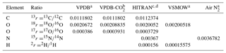
^a Werner and Brand (2001). ^b Brand et al. (2010). ^c Bievre et al. (1984). ^d https://www.cfa.harvard.edu/hitran/molecules.html (last access: 25 October 2018).

Download Print Version | Download XLSX

Isotope ratios are commonly expressed as delta values relative to a standard or reference material:

(Following the recommendation of Coplen (2011) and to simplify equations, the factor 1000 ‰ is not included in the definition of δ.) For the relevant reference scales commonly used in atmospheric analysis, the reference isotope ratios are given in Table 1.

For each isotope of an element, the isotopic abundance or isotopic fraction is the fraction of that isotope relative to all isotopes in a sample:

Note that these are fractional abundances, such that ${}^{\mathrm{12}}x{+}^{\mathrm{13}}x=\mathrm{1}$ and ${}^{\mathrm{16}}x{+}^{\mathrm{17}}x{+}^{\mathrm{18}}x=\mathrm{1}$.

Similarly, the isotopologue abundances or isotopologue fractions are defined for a molecule; for example, for CO₂ the isotopologue abundances for ¹²C¹⁶O₂ (626), ¹³C¹⁶O₂ (636), ¹²C¹⁶O¹⁸O (628) and ¹²C¹⁶O¹⁷O (627) are

where

The labels 626, 636, 628 and 627 are the common isotopic shorthand used in spectroscopy and the HITRAN database (Rothman et al., 2005). The sum of all isotopologue abundances x over all 18 isotopologues is equal to unity. R_sum is a sum of the 18 products of isotope ratios, one corresponding to each of the 18 possible isotopologues of CO₂. R_sum conveniently accounts for all possible isotopologues in calculations of abundances, providing a normalising factor somewhat analogous to a partition sum over all energy levels of a molecule. From Eq. (4), $x_{\mathrm{626}}=\mathrm{1}/R_{\mathrm{sum}}$ i.e. 1∕R_sum is the fractional abundance of the major isotopologue and $R_{\mathrm{sum}}-\mathrm{1}\approx \mathrm{1}-x_{\mathrm{626}}$ is that fraction of the sample that is made up of all the minor isotopologues. Equivalently, from Eq. (10) and the following paragraph, it can be seen that R_sum is the ratio of the total amount of CO₂ to that of the major isotopologue in a sample.

Table 2Isotopologue fractional abundances and isotopic sums for the VPDB-CO₂ and HITRAN scales and conversion factors.

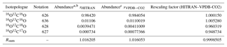
Abundances are taken from ^a Rothman et al. (2005) and ^b https://www.cfa.harvard.edu/hitran/molecules.html (last access: 25 October 2018) for HITRAN and ^c Brand et al. (2010) for VPDB-CO2. The Brand et al. values supersede earlier values given by Allison et al. (1995).

Download Print Version | Download XLSX

Abundances of the major and three singly substituted isotopologues and R_sum values for standard reference materials are given in Table 2. Abundances of the multiply substituted isotopologues can be calculated following the examples of Eq. (4). They are also listed for HITRAN isotope ratios on the HITRAN website: https://www.cfa.harvard.edu/hitran/molecules.html (last access: 25 October 2018).

For a calibration or reference gas, δ¹³C and δ¹⁸O are usually provided by calibration laboratories, and δ¹⁷O can normally be deduced from δ¹⁸O, assuming mass dependent fractionation of oxygen isotopes with negligible error (Brand et al., 2010):

The mass dependent fractionation assumption is discussed below in Sect. 6. The isotope ratios ¹³r,¹⁷r and ¹⁸r for a sample can thus be calculated from inverting Eq. (2):

thence R_sum can be calculated from Eq. (5) for any sample or reference gas.

If the total mole fraction of CO₂ in a sample of air, $y_{{\mathrm{CO}}_{\mathrm{2}}}$, is also known (for example, for a certified calibration gas), the individual isotopologue amounts or mole fractions can be calculated from

(Following the recommendation of the IUPAC Gold Book (McNaught and Wilkinson, 2014) and usage by Tans et al. (2017), the symbol y is used here for mole fraction (more formally amount fraction) of a trace gas or isotopologue in air to distinguish from x, the isotope or isotopologue fractional abundance.)

Conversely, if a set of calibrated isotopologue mole fractions $\mathit{\{}{y}_{\mathrm{626}},y_{\mathrm{636}},y_{\mathrm{628}},y_{\mathrm{627}}\mathit{\}}$ in a sample are measured with an isotopologue-specific analyser, the total CO₂ mole fraction $y_{{\mathrm{CO}}_{\mathrm{2}}}$and isotope ratios or delta values can be calculated. The isotope ratios are derived directly from the isotopologue amounts:

Then delta values are calculated from Eq. (2) and R_sum from Eq. (5). The total CO₂ mole fraction is then calculated from Eq. (8):

The key quantity in these calculations is R_sum, which correctly and completely accounts for all possible isotopologues of the molecule at their actual isotopic abundances. Note that to correctly calculate the amount of any isotopologue in a sample, all isotope ratios should be known to calculate R_sum exactly. Errors incurred when this requirement is relaxed are discussed and quantified in Sect. 5.

In the HITRAN database, tabulated line strengths are normalised by the natural abundance of the relevant isotopologue; the reference isotopologue natural abundances assumed in HITRAN are listed in Table 2. Retrievals from spectra based on HITRAN line parameters thus provide scaled or normalised mole fractions of isotopologues, which are referenced to the isotopic scales assumed by HITRAN. For some purposes it may be convenient to work with these normalised mole fractions directly rather than convert them to absolute mole fractions as in Sect. 2 because the reference isotopologue abundances are inherently included in the normalised amounts. In terms of normalised mole fractions, Eq. (8) becomes

where r_ref and R_sum,ref refer to the reference scales listed in Tables 1 and 2 and $X_{\mathrm{sum}}=R_{\mathrm{sum}}/R_{\mathrm{sum},\mathrm{ref}}=R_{\mathrm{sum}}\cdot x_{\mathrm{626},\mathrm{ref}}$. Equation (11) allows normalised mole fractions to be calculated the from total CO₂ mole fraction and δ values on any reference scale for which r_ref and R_sum,ref are known.

The calculation of δ values from normalised isotopologue mole fractions is analogous to Eqs. (9) and (10):

and the total CO₂ mole fraction is

The normalised mole fractions have the convenient property that they are all equal to the total CO₂ mole fraction in a sample if all isotopes are in natural abundance in the reference scale (i.e. Eq. 11 with δ=0, $R_{\mathrm{sum}}=R_{\mathrm{sum},\mathrm{ref}}$ and X_sum=1). HITRAN natural abundances are based on a superseded definition of the VPDB isotope ratio for carbon and VSMOW for oxygen, while for atmospheric CO₂ the isotopic scale of choice is VPDB-CO₂, which is based on VPDB for both carbon and oxygen and may be adjusted over time as scales are redetermined. To convert normalised mole fractions retrieved directly from spectra (HITRAN scale) to the VPDB-CO₂ scale, each normalised mole fraction can be multiplied by $x_{\mathrm{ref},\mathrm{Hitran}}/x_{\mathrm{ref},\mathrm{VPDB}}$. The reference isotopologue abundances and rescaling factors are listed in Table 2.

Calibration of an isotopologue-specific analyser can in principle be carried out in two ways: calibrating on either the individual isotopologue amounts or on the derived isotope ratios or delta values. Both methods have been used in published work to date. The former is more fundamental because optical methods actually measure individual isotopologue amounts, not ratios. Ratio- or delta-based calibration leads to the additional complication of concentration dependence in the calibration. A step-by-step method for direct isotopologue calibration is presented in Sect. 4.1 based on the equations of Sect. 2. Ratio or delta calibration is discussed in Sect. 4.2 and the two methods are compared in Sect. 4.3.

4.2 Calibration by delta values

Spectroscopic analysers fundamentally determine the amounts of individual isotopologues, and the isotopologue-based analysis as described in the preceding section is the natural choice as a basis for calibration. Historically, however, isotope ratio mass spectrometry (IRMS) has been the method of choice for isotopic analysis because many sources of noise cancel in calculating the ratio. Traditional IRMS calibration schemes are based on standards over a range of isotope ratios or delta values directly, rather than on isotopologue amounts. Ratio or delta calibration schemes have thus, perhaps inevitably, flowed through to optical techniques. Ratio calibration schemes use calibration standards which cover a range of delta values and derive calibration equations analogous to Eq. (14) directly in terms of delta values rather than isotopologue amounts. The raw measured delta values are calculated from the uncalibrated isotopologue amounts. However, as shown in the following, this method inevitably leads to a concentration dependence of the calibration equations, which must be characterised as part of (and which significantly complicates) the calibration procedure.

Several groups have reported on ratio calibration schemes and the consequent concentration dependence (e.g. Griffith et al., 2012; Wen et al., 2013; Rella et al., 2015; Pang et al., 2016; Braden-Behrens et al., 2017; Flores et al., 2017). The concentration dependence inevitably follows if the actual calibration relationships between measured and true amounts of individual isotopologues (Sect. 4.1, Eq. 14) have a non-zero y intercept or an additional non-linear term. Griffith et al. (2012, Eq. 14) showed that a non-zero intercept in the calibration equations leads to an approximate inverse dependence of measured δ¹³C on concentration. Extending that to include a quadratic term in the calibration equation representing non-linearity adds an approximately linear term to the concentration dependence, which can then be described by a combination of an inverse and linear dependence on $y_{{\mathrm{CO}}_{\mathrm{2}}}$:

$$\begin{array}{}\text{(15)}& {{\mathit{\delta }}^{\mathrm{13}}\mathrm{C}}_{\mathrm{meas}}=\mathit{\alpha }\cdot {{\mathit{\delta }}^{\mathrm{13}}\mathrm{C}}_{\mathrm{true}}+(\mathit{\alpha }-\mathrm{1})+{\displaystyle \frac{\mathit{\beta }}{y_{{\mathrm{CO}}_{\mathrm{2}}}}}+\mathit{\gamma }\cdot y_{{\mathrm{CO}}_{\mathrm{2}}},\end{array}$$

where δ¹³C_meas is calculated from the raw measured isotopologue amounts. For a perfectly linear calibration, i.e. Eq. (14) with $b_{\mathrm{626}}=b_{\mathrm{636}}=\mathrm{0}$, both β and γ are zero, $\mathit{\alpha }=a_{\mathrm{636}}/a_{\mathrm{626}}$ and Eq. (15) represents a simple concentration-independent scale shift of (α−1) in the δ scale. β is a function of the intercept terms b₆₂₆ and b₆₃₆. γ becomes non-zero if quadratic terms are added to the calibration equations. The inverse and linear $y_{{\mathrm{CO}}_{\mathrm{2}}}$ dependences are not exact because the coefficients β and γ contain terms dependent on δ¹³C and also have weak cross-terms, but together they provide a useful model to describe the concentration dependence. The linear term becomes relatively more important than the inverse term at high CO₂ mole fractions, where the inverse CO₂ term becomes small, and any quadratic contribution to the calibration equation leading to the linear term becomes large.

Figure 1 illustrates this concentration dependence with a typical δ¹³C vs. CO₂ dependence for an FTIR analyser similar to that used in the example of Sect. 5 below. The dependence was determined by continuous flow measurements of a single CO₂-spiked air tank while the CO₂ content was gradually reduced by passing a fraction of the flow through Ascarite. The measured δ¹³C vs. CO₂ data are fitted to Eq. (15) with fitted parameters $\mathit{\beta }=-\mathrm{1227}$ ‰ ppm and γ=0.0054 ‰ ppm⁻¹, corresponding to CO₂ dependent corrections of up to 5 ‰ over the CO₂ range of 400–1000 ppm. The residuals of the fit illustrate potential errors from the modelled behaviour of up to ±0.3 ‰. Uncertainties in calibrating the CO₂ concentration dependence can lead to significant errors in Keeling-type analyses over a wide range of total CO₂ amounts even if the isotopologue calibration non-linearity is very small (Pang et al., 2016; Wen et al., 2013).

Figure 1Example of δ¹³C dependence on CO₂ mole fraction for a Spectronus FTIR analyser. The measured data are fitted with a function of form of Eq. (15) with fitted parameters $\mathit{\beta }=-\mathrm{1227}$ ‰ ppm and γ=0.0054 ‰ ppm⁻¹.

Download

The concentration dependence is a function of the isotopologue calibration coefficients, and thus in principle for best accuracy it should be redetermined for every calibration, complicating the calibration procedure. The Thermo Fisher Delta Ray isotope analyser, for example, takes this approach in a prescribed sequence of measurements using several reference standards; however, Braden-Behrens et al. (2017) and Flores et al. (2017) found this procedure not to be sufficiently accurate or stable and invoked separate a posteriori calibration schemes. Rella et al. (2015) and Picarro (2017) similarly describe a calibration procedure for Picarro analysers to take concentration dependence into account.

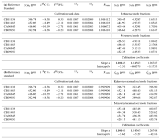
Table 3Worked data for calibration of an FTIR analyser using four reference standards in (a) using actual mole fractions of all isotopologues, and (b) using normalised mole fractions on the VPDB-CO₂ scale. The ¹⁷r and δ¹⁷O values were not directly determined and are not included in the table – they are derived from ¹⁸r and δ¹⁸O following Eq. (6).

Download Print Version | Download XLSX

This section presents a worked example of the calibration of an optical analyser using reference gases of given total CO₂ mole fraction, δ¹³C and δ¹⁸O, followed by measurements of air to which this calibration is applied. The data are derived from an Ecotech Spectronus FTIR analyser which measures three isotopologues of CO₂ (626, 636, 628) in the calibration gases and in the sampled air. The calculations follow Sect. 4.1.

5.1 Calibration

The calibration data were collected in the laboratory at the University of Wollongong on 27 September 2017. Four reference tanks were sourced from CSIRO, with total CO₂ mole fraction, δ¹³C and δ¹⁸O provided on the current WMO reference scales (WMO X2007 scale for total CO₂, VPDB-CO₂ for δ¹³C and δ¹⁸O). For each calibration tank, ${}^{\mathrm{13}}r{,}^{\mathrm{18}}r{,}^{\mathrm{17}}r$, R_sum and reference isotopologue mole fractions are calculated from Eqs. (7), (5) and (8). The four reference gases were measured in the analyser, and raw measured values of the isotopologue mole fractions were corrected to dry air and for small spectroscopic cross-sensitivities to pressure, temperature and water vapour, as described by Griffith et al. (2012). A two-parameter linear regression (slope and intercept) of measured against reference mole fractions for each isotopologue provides the linear calibration coefficients a and b for the analyser, Eq. (14). The worked data are presented in Table 3 and calibration plots shown in Fig. 2.

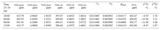
Table 4Worked calibration of sample data in Fig. 3 at four times with varying CO₂ mole fractions. Columns 2–4 contain the raw measured isotopologue mole fractions corrected to dry air, columns 5–7 contain the calibrated dry air mole fractions after applying the coefficients from Table 3, columns 8–10 are the isotopic ratios and R_sum for each sample, and columns 11–13 contain the final calibrated total CO₂, δ¹³C and δ¹⁸O.

Download Print Version | Download XLSX

Figure 2Calibration plots for three CO₂ isotopologues.

Download

5.2 Sample air measurements

Figure 3 shows an example of 1 day of calibrated 1 min measurements from the same FTIR analyser collected at a rural site in SE Australia on 23 and 24 January 2018. Table 4 illustrates the worked calibration of the raw data at four times of differing CO₂ amounts and isotopic fractionations. The linear calibration of 27 September 2017 described above has been applied to the measured data without further correction. The calculations follow Sect. 4.1 to determine $y_{{\mathrm{CO}}_{\mathrm{2}}}$, δ¹³C and δ¹⁸O for each 1 min measurement. Figure 4 shows an example of a Keeling plot derived from the data of Fig. 3, with an intercept −24.5 ‰ typical of the dominant plants in this agricultural area.

Table 5Actual isotopologue amounts and R_sum values in 400 ppm total CO₂ for various isotopic compositions. The last column lists errors in calculating total CO₂ if different isotopic composition between reference (calibration) and sample measurements are not accounted for. See text for details of the various cases.

Download Print Version | Download XLSX

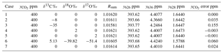
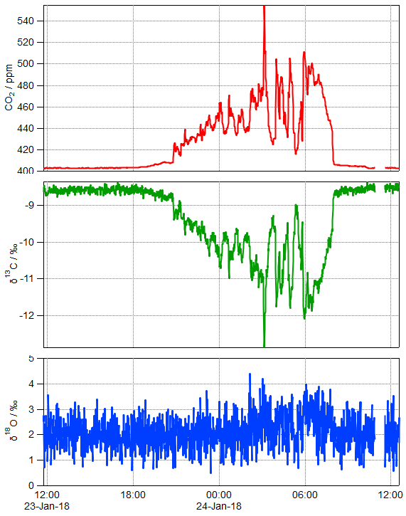
Figure 3Calibrated total CO₂, δ¹³C and δ¹⁸O of sampled air on 23–24 January 2018 at a rural site in SE Australia. Air was sampled continuously, and the displayed data are 1 min averages.

Download

Table 5 shows examples of actual isotopologue amounts for samples with total CO₂=400 ppm and a range of isotopic compositions. The table includes R_sum values calculated for each sample. The potential error incurred in calculating the total CO₂ amount from a spectroscopic measurement of y₆₂₆ via Eq. (10) if the different isotopic composition between sample and reference gases is not taken into account is shown in the rightmost column – it is the difference from 400 ppm of the total CO₂ calculated from Eq. (10) taking the reference value R_sum,ref (case 1) instead of the correct value on the same line R_sum. This simulates the effect of ignoring the difference in isotopic composition between reference and sample. The reference case (case 1) is a hypothetical standard with the isotopic composition of VPDB-CO₂. Examples include typical clean air (case 2), synthetic air synthesised with ¹³C-depleted CO₂ with δ¹³C $=-\mathrm{35}$ ‰ (case 3), systematic errors of 2 ‰ in δ¹⁸O and δ¹⁷O (cases 4, 5), and the use of isotope ratios assumed by HITRAN rather than VPDB-CO₂ (case 6). Case 7 simulates the result if only singly substituted isotopologues are included in the sum and all doubly substituted minor isotopologues are ignored. Other cases can be assessed following the equations of Sect. 2. Potential errors are fortunately small relative to GAW compatibility goals for realistic isotopic variations of a few per mil around clean air values. However the potential for significant errors (> 0.1 ppm) exists for reference gas mixtures or samples with ¹³C-depleted CO₂ as is often the case for synthetic mixtures or for samples with added CO₂ derived from plant or fossil fuel sources.

Figure 4Keeling plot of data shown in Fig. 3.

Download

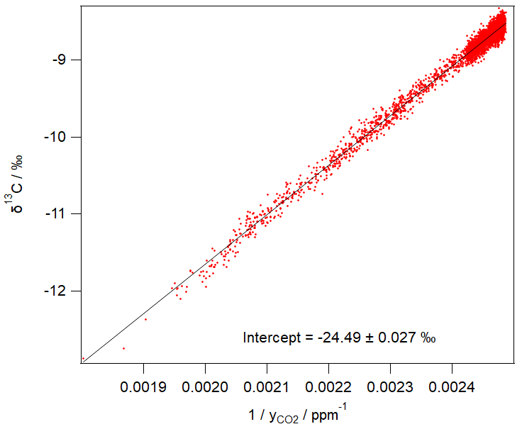
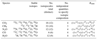
Table 6Details of isotopologues of common atmospheric species.

Download Print Version | Download XLSX

These potential errors in computation of delta values should also be viewed in the context of experimental measurement errors. Flores et al. (2017) formally evaluated the uncertainty budget for their particular FTIR measurements of δ¹³C in CO₂ and found a standard uncertainty of 0.09 ‰, of comparable magnitude to the largest potential computational approximation errors. The measurement uncertainty was dominated by uncertainty in assigned reference mole fractions for the reference standards rather than the spectroscopic measurement uncertainty.

Three assumptions, previously mentioned and summarised here, have negligible impact on the calculations of Sect. 2 and Table 5.

• ¹⁴C, with an isotopic abundance of < 1 ppt is ignored in all calculations.

• The relative amounts of multiply substituted minor isotopologues are assumed to be in statistical relative abundance, i.e. there is no isotope clumping. Clumping refers to the case where the enrichment (or depletion) of two or more isotopes in a multiply substituted isotopologue are correlated, rather than each following their statistical amounts independently. Clumping effects are normally much less than 1 ‰, and according to Table 5 are therefore insignificant.

• Values ¹⁷r and δ¹⁷O are calculated from ¹⁸r and δ¹⁸O (Eq. 6) assuming mass dependent fractionation. Thermodynamic and kinetic fractionation processes are mass-dependent and account for most fractionation mechanisms in nature. Mass-independent fractionation typically occurs in quantum processes such as photolysis and can cause small deviations from mass dependence. These deviations are also typically < 1 ‰ (e.g. Miller et al., 2002) and thus also negligible for the purposes of this work.

Similar considerations apply to other molecular species, see Table 6. For CH₄, ¹³CH₄ measurements are commonly made using laser analysers such as those of Picarro (Rella et al., 2015), and isotopic reference gases are available. An analysis similar to that in Sect. 6 and Table 5 shows that for 2000 ppb CH₄ in air, an error of 10 ‰ in the assumed value of δ¹³C leads to an error of 0.2 ppb in the calculated total CH₄ mole fraction, and for a −35 ‰ error the total CH₄ error is 0.7 ppb. A 100 ‰ error in δ²H leads to an error in total CH₄ of only 0.1 ppb.

For N₂O there is the additional complication of the isotopomers ¹⁵N¹⁴N¹⁶O and ¹⁴N¹⁵N¹⁶O, for which standard reference gases are not available, and for which measurement technologies are currently less advanced. The general magnitude of potential errors will be similar to those of CO₂. For CO, reference gases are available, but current optical techniques are not able to resolve isotopic variations with sufficient accuracy at the typical low total mole fractions in air.

Several commercial manufacturers offer isotopologue-specific optical analysers based on laser (Campbell Scientific, Picarro, Los Gatos Research, Aerodyne Research, Thermo Fisher Scientific) or FTIR (Ecotech) spectroscopy that analyse sampled air for one or more specific isotopologues. These instruments report results in a variety of ways, as isotopologue mole fractions and/or as total mole fractions and isotopic delta values, both calibrated and uncalibrated. In most cases the scheme by which total mole fractions and delta values are calculated from the raw measured data is not fully described, although some details are available in user manuals and published works. In most cases some level of approximation is used in accounting for the full molecular isotopic composition when converting between isotopologue amounts and total amounts and delta values. As shown in Sect. 6, these approximations are fortunately in most cases acceptably small, but it is nevertheless recommended that they be assessed and documented if the full computation scheme is not used or measurement, and calibration data for all isotopologues are not available.

GAW reports on Carbon Dioxide, other Greenhouse Gases and Related Tracers Measurement Techniques since 2011 (WMO-GAW, 2012) recommend that the computational scheme for isotopic quantities derived from all commercial and non-commercial analysers be published and fully transparent to the user to avoid the potential for biases and inaccuracies stemming from different calibration and calculation schemes. Potential errors and calibration biases due to inconsistent isotopic calculations and the empirical determination of concentration dependences can be avoided if only the raw output isotopologue amounts from the analyser(s) are used and calibrated and isotopic quantities are calculated a posteriori following consistent calculation schemes, such as those described here and in Flores et al. (2017) and Tans et al. (2017).

Data in the paper are only illustrative of the calculations. There are no original or published data.

The author is a consultant to Ecotech Pty Ltd., manufacturer of the Spectronus trace gas analyser under licence to the University of Wollongong.

This article is part of the special issue “The 10th International Carbon Dioxide Conference (ICDC10) and the 19th WMO/IAEA Meeting on Carbon Dioxide, other Greenhouse Gases and Related Tracer Measurement Techniques (GGMT-2017) (AMT/ACP/BG/CP/ESD inter-journal SI)”. It is a result of the 19th WMO/IAEA Meeting on Carbon Dioxide, Other Greenhouse Gases, and Related Tracer Measurement Techniques (GGMT-2017), Empa Dübendorf, Switzerland, 27–31 August 2017.