the Creative Commons Attribution 4.0 License.
the Creative Commons Attribution 4.0 License.
 | 19 Nov 2018
Machine learning for improved data analysis of biological aerosol using the WIBS
Simon Ruske
David O. Topping
Virginia E. Foot
Andrew P. Morse
Martin W. Gallagher
Primary biological aerosol including bacteria, fungal spores and pollen have important implications for public health and the environment. Such particles may have different concentrations of chemical fluorophores and will respond differently in the presence of ultraviolet light, potentially allowing for different types of biological aerosol to be discriminated. Development of ultraviolet light induced fluorescence (UV-LIF) instruments such as the Wideband Integrated Bioaerosol Sensor (WIBS) has allowed for size, morphology and fluorescence measurements to be collected in real-time. However, it is unclear without studying instrument responses in the laboratory, the extent to which different types of particles can be discriminated. Collection of laboratory data is vital to validate any approach used to analyse data and ensure that the data available is utilized as effectively as possible.
In this paper a variety of methodologies are tested on a range of particles collected in the laboratory. Hierarchical agglomerative clustering (HAC) has been previously applied to UV-LIF data in a number of studies and is tested alongside other algorithms that could be used to solve the classification problem: Density Based Spectral Clustering and Noise (DBSCAN), k-means and gradient boosting.
Whilst HAC was able to effectively discriminate between reference narrow-size distribution PSL particles, yielding a classification error of only 1.8 %, similar results were not obtained when testing on laboratory generated aerosol where the classification error was found to be between 11.5 % and 24.2 %. Furthermore, there is a large uncertainty in this approach in terms of the data preparation and the cluster index used, and we were unable to attain consistent results across the different sets of laboratory generated aerosol tested.
The lowest classification errors were obtained using gradient boosting, where the misclassification rate was between 4.38 % and 5.42 %. The largest contribution to the error, in the case of the higher misclassification rate, was the pollen samples where 28.5 % of the samples were incorrectly classified as fungal spores. The technique was robust to changes in data preparation provided a fluorescent threshold was applied to the data.
In the event that laboratory training data are unavailable, DBSCAN was found to be a potential alternative to HAC. In the case of one of the data sets where 22.9 % of the data were left unclassified we were able to produce three distinct clusters obtaining a classification error of only 1.42 % on the classified data. These results could not be replicated for the other data set where 26.8 % of the data were not classified and a classification error of 13.8 % was obtained. This method, like HAC, also appeared to be heavily dependent on data preparation, requiring a different selection of parameters depending on the preparation used. Further analysis will also be required to confirm our selection of the parameters when using this method on ambient data.
There is a clear need for the collection of additional laboratory generated aerosol to improve interpretation of current databases and to aid in the analysis of data collected from an ambient environment. New instruments with a greater resolution are likely to improve on current discrimination between pollen, bacteria and fungal spores and even between different species, however the need for extensive laboratory data sets will grow as a result.


Biological aerosol, such as bacteria, fungal spores and pollen have important implications for public health and the environment (Després et al., 2012). They have been linked to the formation of cloud condensation nuclei and ice nuclei which in turn may have important influence on the weather (Crawford et al., 2012; Cziczo et al., 2013; Gurian-Sherman and Lindow, 1993; Hader et al., 2014; Hoose and Möhler, 2012; Möhler et al., 2007). These particles have impacts on health (Kennedy and Smith, 2012), particularly for those who suffer from asthma and allergic rhinitis (D'Amato et al., 2001). It is therefore of paramount importance that we continue to develop methods of detecting these particles, to quantify them, determine seasonal trends and to compare different environments.
There are a wide range of biological molecules, commonly referred to as biological fluorophores, that are known to re-emit radiation upon excitation, e.g. amino acids, coenzymes and pigments (Pöhlker et al., 2012, 2013). Ultraviolet-light induced fluorescence (UV-LIF) spectrometers, such as the wideband integrated bioaerosol spectrometer (WIBS) have received increased attention in recent years as a potential methodology for detecting biological aerosol (Kaye et al., 2005). The WIBS uses irradiation at 280 and 370 nm to target some of the most significantly fluorescent bioflorophores such as tryptophan (an amino acid) and NADH (a coenzyme). These measurements are combined with an optical measurement of size and shape to further aid in discrimination.
Measurements from the WIBS have limited application in isolation. However, there are a range of techniques that could be used to predict quantities of biological aerosol from these fluorescence, size and morphology measurements. Techniques that could be used to solve this classification problem, include field specific techniques such as ABC analysis (Hernandez et al., 2016) as well as supervised and unsupervised machine learning techniques that are broadly used (Friedman et al., 2001).
It is not clear at this point what approach is preferred as all approaches have a range of advantages and disadvantages.
Supervised machine learning uses data collected within the laboratory, where the correct classification is known. Data are split into training data and testing data where the training data are used to fit a model which is then validated on the test set. Once a model is fitted and validated it may then be applied to classify ambient data.
During unsupervised analysis, ambient data are classified without using laboratory training data. Instead, an attempt is made to naturally segregate the data. Ideally, we may expect data to naturally be segregated into broad biological classes or into different groups of similar bacteria, fungal material and pollen, but this may not necessarily be the case.
The supervised methods, have the disadvantage that training data collected may not include the entirety of what might be collected during an ambient campaign. Particularly, in an urban environment, the instrument may collect measurements for a large quantity of non-biological material that should be classified as such or removed from the analysis. We would expect most of this non-biological material to either be non-fluorescent or weakly fluorescent and therefore it should be removed prior to analysis by applying a justifiable threshold to the fluorescent measurements (see Sect. 2.2). Nonetheless, a few weakly fluorescent non-biological particles may remain and could be overlooked if the training data are incomplete.
There are likely to be issues to be explored with either approach and therefore it seems unlikely that either supervised or unsupervised techniques can justifiably be abandoned at this point in time and it may well be the case that usage of a variety of techniques may be required to better understand the atmospheric environment. Nonetheless, it is still vital to investigate how these different techniques behave when analysing laboratory data to better understand how they can be most appropriately applied to ambient data.
In an ambient setting, determining the number of clusters is difficult, so hierarchical agglomerative clustering (HAC) has been the preferred method over other methods such as k-means since the method naturally presents a clustering for all possible number of clusters (Robinson et al., 2013). A suggestion of the number of clusters can then be provided using indices such as the Caliński–Harabasz Index (CH Index) (Caliński and Harabasz, 1974) by maximizing a statistic which yields a peak for clusterings which contain clusters that are compact and far apart. HAC has previously been used on data collected using the WIBS to discriminate between different Polystyrene Latex Spheres (PSLs) and has been applied to ambient measurements collected as part of the BEACHON RoMBAS experiment (Crawford et al., 2015; Gabey et al., 2012; Robinson et al., 2013).
Nonetheless, relatively few studies have studied the usage of HAC on laboratory data from the WIBS (Savage and Huffman, 2018; Savage et al., 2017). Evaluating the effectiveness of HAC on generated aerosol is crucial to support or repudiate conclusions made using HAC on ambient data, especially since the fluorescence response from the laboratory generated aerosol will much better reflect fluorescence responses from the environment, when compared with PSLs.
During the process of HAC there are also a number of vital choices that have to be made that could have a substantial implication on the effectiveness of the method (these are discussed in detail in Sect. 2.2). For the PSLs previously analysed (Crawford et al., 2015), we determined standardizing using the z score, with removal of non-fluorescent particles, taking logarithms of shape and size was most effective. The CH index was selected to determine the number of clusters as it was demonstrated to perform best in the literature (Milligan and Cooper, 1985). It is, however, not clear whether these choices will remain the most effective for laboratory generated aerosol or ambient data. See Sect. 2.3 for further details on data preparation for HAC.

Furthermore, data analysis using HAC can take a matter of hours, if not days, depending on the number of particles. The time requirements for HAC are between N2 and N3 meaning that a doubling of the number of particles will require between 4 and 8 times as much time. Such time requirements mean that not only is the method already quite slow, but will get increasingly slower as more data are collected, which may limit the real time effectiveness of the method.
Within the Python programming language, a package called Scikit-learn (Pedregosa et al., 2011) offers implementations of several unsupervised methods. Some of these methods, i.e. Affinity Propagation, Mean-shift, Spectral Clustering and Gaussian mixtures are not explored as they will scale poorly as the number of particles increases (Pedregosa et al., 2011). Instead, our analysis is focused on k-means, HAC and DBSCAN which can be used on larger data-sets.
For HAC we continue to use the fastcluster package (described in Sect. 2.3). Sci-kit learn does have a HAC implementation but it is not as fast or memory efficient. We do use sklearn for DBSCAN and k-means, although if one was to use DBSCAN for ambient data we would suggest exploring alternatives such as ELKI (Schubert et al., 2015) as the sci-kit learn implementation of DBSCAN by default is not memory efficient making it difficult to utilize for more than 30 000 particles. Sci-kit learn has a fast implementation for gradient boosting, so this is used.
In this section we discuss the variety of approaches that could be used to classify particles such as bacteria, fungal spores or pollen. In Sect. 2.1 we provide an overview of the instrument used to collect the data. In Sect. 2.2 we discuss the variety of decisions that need to be made prior to passing the data to the machine learning algorithms which are discussed in Sect. 2.3–2.6. An overview of the different methods is given in Fig. 1.
2.1 Instrumentation
The Wideband Integrated Bioaerosol Sensor (WIBS) collects size, shape and fluorescence measurements (Kaye et al., 2005). The size is a single measurement; the shape measurement consists of four measurements (one for each quadrant) which are combined to produce a single asymmetry factor measurement. A more precise definition of asymmetry factor has been provided previously in the literature (Gabey et al., 2010).
To measure fluorescence, the particle is irradiated with UV light at 280 and 370 nm from the firing of two xenon sources. Fluorescence emission is collected via two collection channels in the ranges 310–400 and 420–600 nm. The 370 nm xenon radiation lies within the first detection range and hence elastically scattered light from the particle, sufficient to saturate the detection amplifier, is received. This signal is therefore discarded.
After removal of this fluorescent measurement, there are three remaining fluorescence measurements. The notation FL1_280 is used to denote the measurement in the first detection channel when the particle is irradiated with ultraviolet light at 280 nm and FL2_280 and FL2_370 are used to denote the measurements in the second detection channel when the particle is irradiated with ultraviolet light at 280 and 370 nm, respectively. These fluorescence measurements are combined with the size and asymmetry factor measurements. A more detailed description of the instrument can be found in previous publications (Gabey et al., 2010; Healy et al., 2012a).

2.2 Data preparation
Prior to analysis using the machine learning algorithm we may choose to make a variety of decisions to pre-process the data with the aim to improve performance (see Fig. 2). An overview for the decisions often made are outlined below.
First we may elect to remove particles which are non-fluorescent. Forced trigger data are collected which is a measurement of the instrument response when particles are not present. We then set a threshold, for which if a particle fails to exceed this threshold in at least one of the fluorescent channels we conclude that the particle is non-fluorescent. Usually we set the threshold to be three standard deviations above the average forced trigger measurement although a recent laboratory study has suggested that nine standard deviations may be more appropriate (Savage et al., 2017).
Another threshold is usually then applied to the size. A size threshold of 0.8 µm is usually applied as detection efficiency of the instrument drops below 50 % at this point. (Gabey, 2011; Gabey et al., 2011; Healy et al., 2012b).
Natural logarithms of the size and the asymmetry factor are often taken as these measurements are often log normally distributed and it is postulated that this will increase performance in the case of hierarchical agglomerative clustering.
It is also widely regarded that standardizing the data prior to analysis is utmost importance (Milligan and Cooper, 1988). We often subtract the average measurement in each of the five variables and divide by the standard deviation, often referred to as “standardizing using the z score”. Standardization is used to prevent variables with larger magnitude, such as the fluorescent measurements, from dominating the analysis. An alternative approach to standardizing is to divide each of the five variables by the range.
2.3 Hierarchical agglomerative clustering
In order for particles to be clustered, we need to define a measurement of how similar two clusters are. These similarity measures are often referred to as linkages. We use the Python package fastcluster (Müllner, 2013) which provides modern implementations of single, complete, average, weighted, Ward, centroid and median linkages (Müllner, 2011). A thorough detailing of the definitions of the different linkages can be found in the fastcluster manual (Müllner, 2013). For the memory efficient mode, which is essential when using the algorithm for large data sets, only Ward, centroid, median and single linkages are available.
Initially each particle is placed into an individual cluster. Next, using the linkage selected, the two most similar clusters are merged. The merging process is repeated until all the particles are placed in a single cluster, which provides a clustering from k=1, …, N, where k is the number of clusters and N is the number of particles being analysed. A cluster validation index such as the Calińnski–Harabasz index (Caliński and Harabasz, 1974) is then used to identify an appropriate number of clusters. The index is maximized for clusterings that contain compact clusters that are far apart.
2.4 K-means clustering
K-Means clustering is designed to place particles into k clusters. However we can repeat the method multiple times, e.g. for k=1, 2, …, 10, where k is the number of clusters. Similar to HAC we can then use a cluster validation index to determine which choice of k gives the most effective results.
The method works as follows. Initially k cluster centroids are set by selecting k particles at random. The rest of the particles are then placed into these k clusters depending on which of the centroids the particle is closest to. At this point a new centroid is calculated for each cluster. The process is then repeated many times until convergence occurs and the centroids do not change significantly from one iteration to the next.
2.5 DBSCAN
For DBSCAN we set two parameters, the radius for a neighbourhood ϵ, and the number of particles required for a neighbourhood to be identified as dense.
Initially a random point, say A, is selected. If there are sufficient number of points in the neighbourhood of A then all the points in A's neighbourhood are also checked and so on, until the cluster has fully expanded and there are no points left to check. Should the point not have a sufficient number of other points in its neighbourhood then it is left unclassified. Further points are then selected and the above process is repeated until all points have been considered.
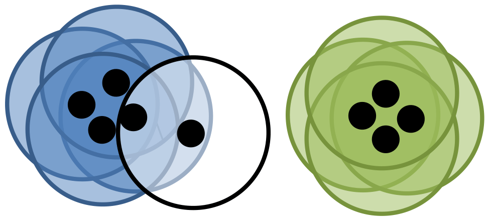
Figure 3Visual representation of DBSCAN. Here each point is represented as a black dot and its neighbourhood is represented by a circle. Here ϵ is the radius of the circle and the minimum number of points is 3. Four points have each been placed into the blue cluster and green cluster, all of which having at least 3 other points in their neighbourhood. One point is classified as noise as it has only 1 other point in its neighbourhood.
We give an example of DBSCAN in Fig. 3. Note that cluster validation indices are not required for DBSCAN, since the number of clusters is intrinsically calculated within the algorithm.
2.6 Gradient boosting
A basic decision tree is constructed by considering each possible split across all variables and evaluating which split best divides the data. For example, we may consider the third fluorescence channel and split the data on the basis of whether the measurement is more or less than 10 arbitrary units (AU). This process is then repeated many times until a tree is built.
There are two ways in which trees can be combined into an ensemble. The first is by averaging multiple trees in the hope to produce a more accurate classification as is the case in random forests and bagging classifiers (Breiman, 1996, 2001). In the case of random forests and bagging, the data set is sampled with replacement, meaning that the same particle could be selected more than once or not at all. Sampling in this way enables the algorithm to produce a subtly different version of the data from which to build each tree. In addition, when using a random forest, instead of considering all possible variables to use to split the data, only a random subset is used.
Alternatively we can fit a single decision tree to the data, evaluate where the tree is performing well and then fit a second tree to the particles in the data for which the current model is performing poorly. This process can be repeated many times, each time adding a new tree to the model in the hope of making an improvement. This approach is known as AdaBoost (Freund and Schapire, 1997). Gradient boosting is an extension of AdaBoost to allow for other loss functions (Friedman, 2001).
For the current study we elect to use gradient boosting to indicate the performance of the supervised approach since it was the best performer for the Multiparameter Bioaerosol Spectrometer, a similar UV-LIF spectrometer similar to the WIBS but with single waveband fluorescence, 8 fluorescence detection channels and very high shape analysis capability (Ruske et al., 2017).
2.7 Evaluation criteria
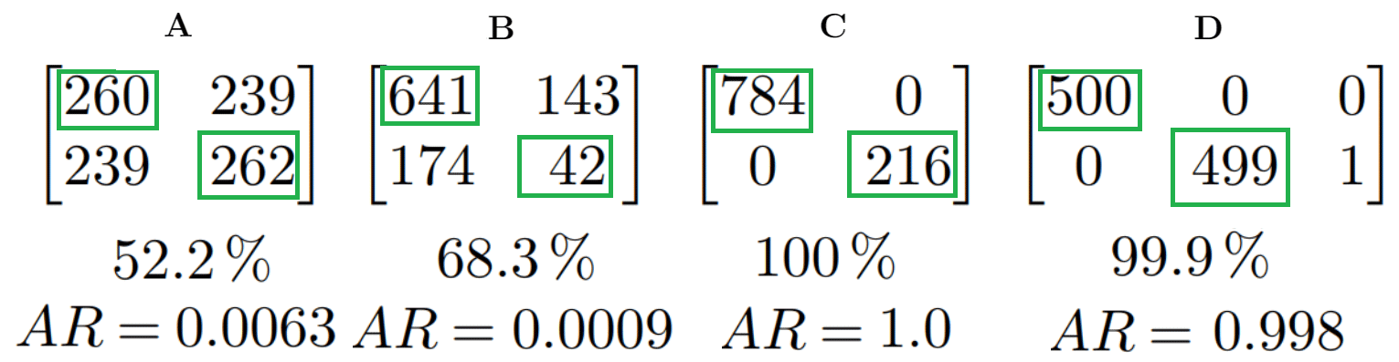
Figure 4Four example matching matrices. Immediately below each matrix is the percentage of particles placed into the same cluster for both clusterings in each case. At the very bottom we have the adjusted rand score.
To aid in evaluating how well methodologies performed we used two tools: the matching matrix (Ting, 2010) and the adjusted rand score (Hubert and Arabie, 1985).
In Fig. 4 we present four different matching matrices. To produce these matrices we compared: two random clusterings with approximately 50 % of the data in each cluster (A); two random clusterings each with 80 % and 20 % of the data in each of the two clusters, respectively (B); two identical clusterings (C); and two clusterings which were nearly identical except one data point had been placed into a third cluster for one of the clusterings.
2.7.1 Matching matrix
The matching matrix, often referred to as a confusion matrix, can be used as an aid in comparing two clusterings.
In the case of the current paper, we use this to compare the output from an algorithm with labels assigned to each particle. We may assign labels to indicate what broad type the particle is (e.g. 1 if the particle is bacteria, 2 if the particle is fungal etc.) or we may assign labels to indicate what sample a particle is from (e.g. 1 if the particle is Bacillus atrophaeus, 2 if the particle is E. coli etc.)
Consider example C in Fig. 4. This matching matrix compares two clusterings each containing two clusters. Each row corresponds to a cluster in the first clustering and each column corresponds to a cluster in the second clustering. The element in the first row and the first column (in this case 784) indicates the number of particles that were placed into the first cluster in the first clustering that were also placed into cluster 1 in the second clustering. Two identical clusterings will produce a matching matrix that has non-zero values only the diagonal.
A and B in Fig. 4 are examples of poor performance and C and D are examples of very good performance.
2.7.2 Adjusted Rand score
When evaluating a large number of clusterings, it may be useful to use a statistic to summarize the information in the matching matrix. In a previous study (Ruske et al., 2017), we used percentage of particles correctly classified as a statistic for indicating performance. This is an easy to interpret statistic, but can be misleading when used on imbalanced data. In both example A and B, we have two randomly generated clusterings. However in B we have 80 % of the data points placed into the first cluster, whereas in A the data points are approximately equally distributed between the two clusters. The percentage of points which are placed into the same cluster for both clusterings are 52.2 % and 68.3 % for A and B, respectively. We can see that the more imbalanced a data set is, the more likely data points are to be placed into the same clusters. It is for this reason we elect to use an alternative statistic: the adjusted rand score. This statistic attains a value of approximately zero for both A and B.
Comparing clusterings is a developing area of research and there are other alternative statistics such as the mutual information score (Vinh et al., 2010) that could be preferable to the adjusted rand score. However our initial tests (not presented), indicated that calculation of the mutual information often required an order of magnitude more time than the calculation of the adjusted rand. Therefore, we elected to use the adjusted rand score for the current study.
The efficacy of the different data analysis approaches was evaluated using three different data sets. The first of which comprised several industry standard polystyrene latex spheres of various different sizes and colours. This data set was first analysed in Crawford et al. (2015), where hierarchical agglomerative clustering was successfully applied to the data yielding a classification accuracy of 98.2 %. This data set presents a simple challenge for which we would expect any reasonable algorithm to be able to discriminate between the different sizes and colours of particles.
To further extend the previous analysis in Crawford et al. (2015) we include two data sets collected in 2008 and 2014 which are similar to data previously published using the Multiparameter Bioaerosol Spectrometer (Ruske et al., 2017). A subsection of the data collected 2014 has previously been analysed in the Appendix of Crawford et al. (2017). These data sets consist of various different pollen, fungal, bacterial and non-biological samples, and should present a much more difficult challenge for the algorithms.
The samples of laboratory generated aerosol were collected as follows. Material was aerosolized into a large, clean HEPA filtered chamber, which incorporated a recirculation fan. The Bacillus atrophaeus and Escherichia coli (E. coli) bacteria were aerosolized into the chamber using a mini-nebulizer (e.g. Hudson RCI Micro-Mist nebulizer) as were the salt and phosphate buffered saline samples. The dry samples, which included the pollen, and fungal samples were aerosolized directly into the chamber from small quantities of powder utilizing a filtered compressed air jet. The diesel smoke and grass smoke samples were generated by burning a small amount within a fume cupboard using a smoker (a piece of bespoke equipment). The bacterial samples were either washed or unwashed and diluted or undiluted.
Table 1The number of particles remaining after a fluorescent threshold of 3σ or 9σ was applied for each of the bacterial samples collected in 2008. Each sample was either washed or unwashed and diluted or undiluted. Each sample was either washed or unwashed, and diluted or undiluted as indicated by a check mark in the corresponding column.
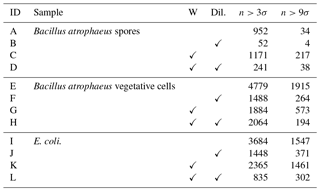
Table 2The number of particles remaining after a fluorescent threshold was applied for each of the non-bacterial samples collected in 2008.
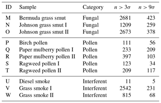
Table 3The number of particles remaining after a fluorescent threshold was applied to each of the samples collected in 2014. Whether a bacterial sample was washed or unwashed is specified after the sample name.
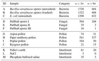

Figure 5Average fluorescent characteristics for the bacterial samples collected in 2008. The error bars in red indicate a range of ±1σ for each sample.
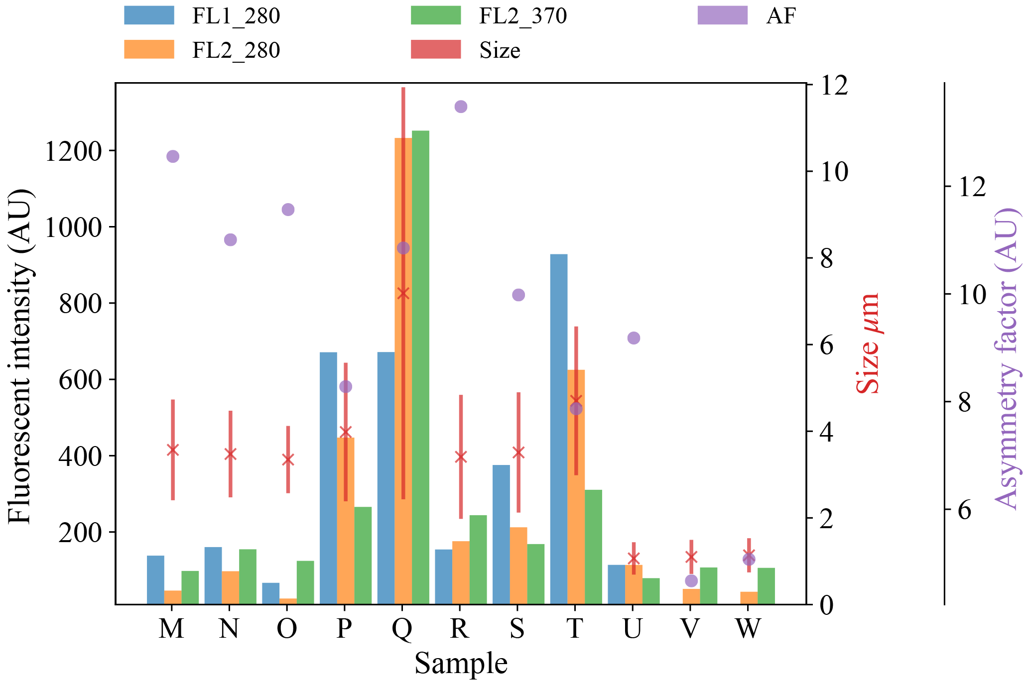
Figure 6Average fluorescent characteristics for the remaining samples collected in 2008. The error bars in red indicate a range of ±1σ for each sample.
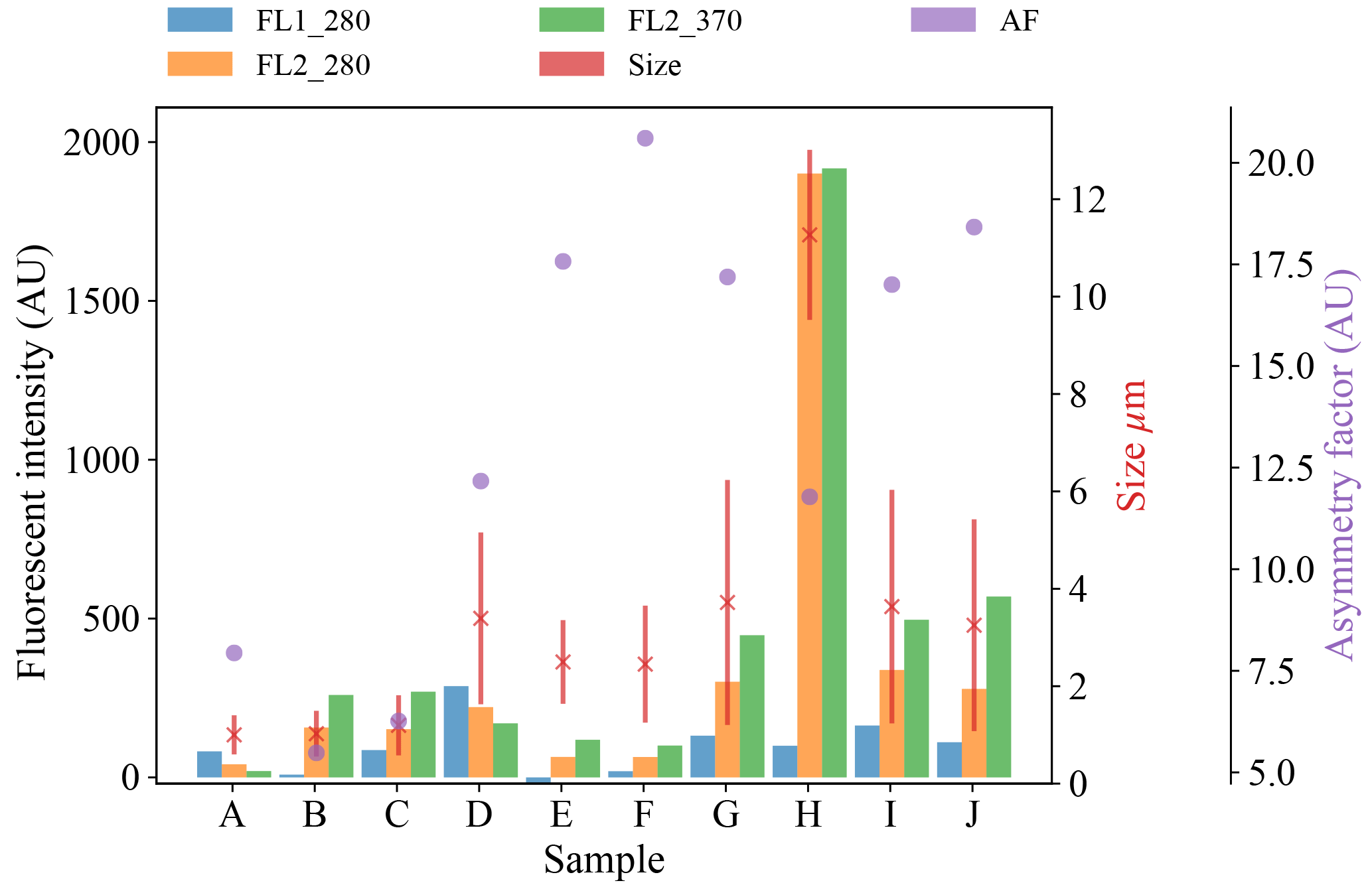
Figure 7Average fluorescent characteristics for the different aerosol samples collected in 2014. The error bars in red indicate a range of ±1σ for each sample.
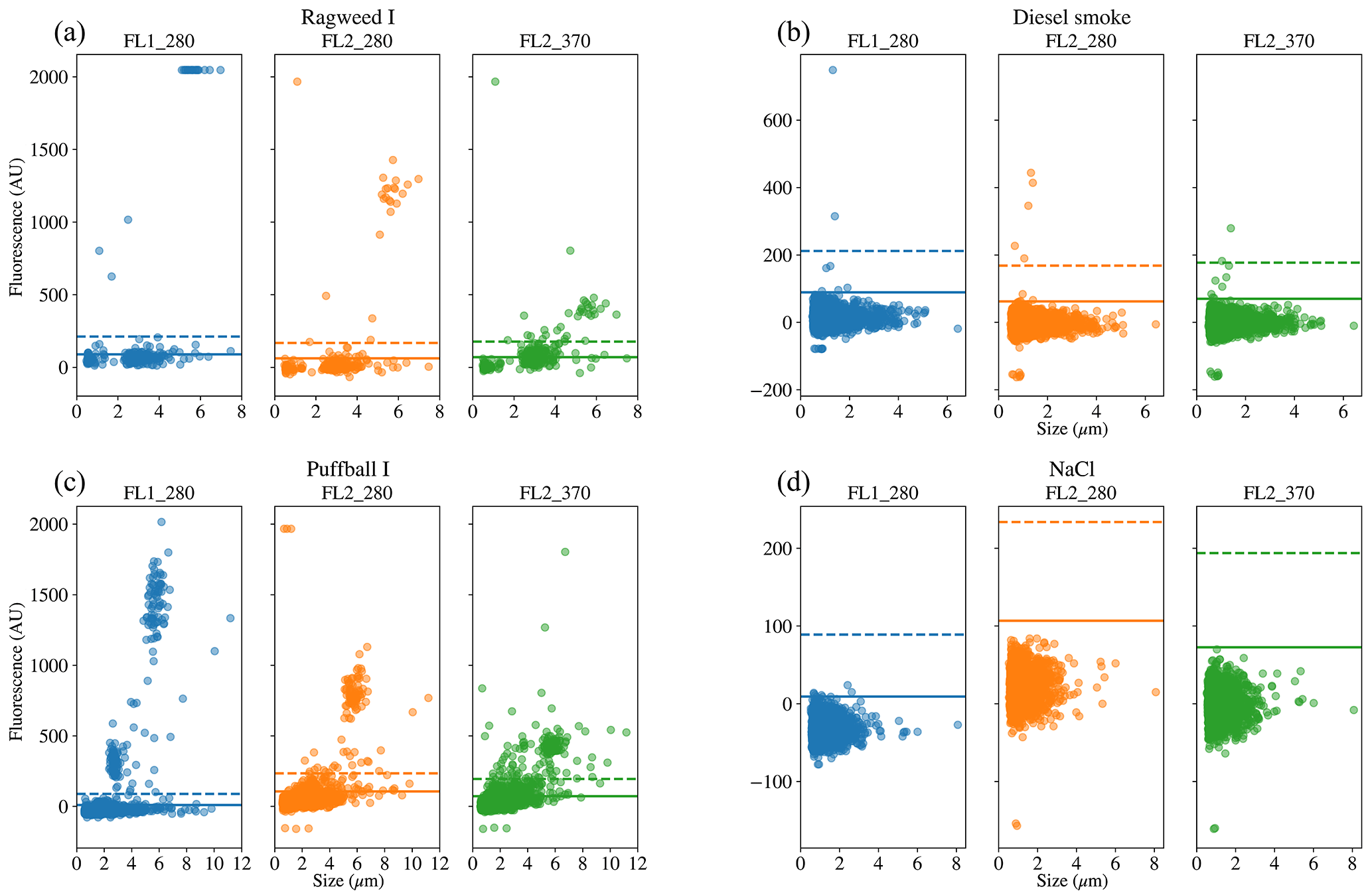
Figure 8Scatter plots of fluorescence vs. size for four of the samples. Two of the samples were collected in 2008 (a, b) and two were collected in 2014 (c, d); two are biological (a, c) and two are non-biological (b, d).
We present a summary of the number of particles for each sample after a fluorescent threshold of 3σ and 9σ is applied in Tables 1, 2 and 3. In 2008 the thresholds are constructed using forced trigger data collected at the same time as the experiment, whereas in 2014 the thresholds are constructed using forced trigger data collected using the same instrument at an earlier date. Ideally, the threshold for the data collected in 2014 would be constructed using forced trigger data collected at the same time as the laboratory data, but we can see in Fig. 8 that the threshold we have constructed is successful in removing the vast majority of NaCl samples collected.
Plots of the average fluorescent characteristics and size and shape for each sample are provided in Figs. 5, 6 and 7 after a fluorescent baseline of 3σ has been applied. Similar plots have been produced using a 9σ threshold and can be found in the repository released alongside the paper (see the “Code and data availability” section for further details). Plots and tables for the polystyrene spheres previously published in Crawford et al. (2015) are omitted.
To provide further clarity on the variation of the samples in terms of size and fluorescence we include scatter plots of each of the fluorescence channels against size for four of the samples in Fig. 8. For the puffball spore and rye grass samples, in particular we can see that we may be measuring both fragmented and intact particles. For the interferent samples we see that a threshold of 3σ removes the vast majority of these particles. In fact the only interferent samples to measure a number of particles over a threshold of 3σ were the grass smoke samples.
The data collected is using a WIBS version 3 which is limited to a detection range of approximately 0.5–12 µm, which limits the ability of the instrument to detect intact pollen grains. The vast majority of the equivalent optical diameters (EODs) for the pollen samples collected are much lower than the measurements for intact pollen grains and are therefore likely to be pollen fragments, as was the case in Hernandez et al. (2016). The exception is the paper mulberry samples where there are differences across each of the samples. In 2008, sample Q which shows a size range similar to the other pollen samples is most likely to consist entirely of pollen fragments, whereas sample R shows a much wider size range which is likely to comprise of both fragmented and intact pollen. The collection of both fragmented and intact pollen has previously been shown to occur in Savage et al. (2017). In 2014, for sample H, the size range is much larger, consistent with the hypothesis of measuring intact pollen. Paper mulberry has been previously been sampled in Healy et al. (2012a), using a WIBS version 4 in a low-gain mode which allows for the collection of particles up to approximately 31 µm. In this study, the size range of the paper mulberry was 13.6±6.2, indicating that if sample H is intact pollen we may only be measuring part of the distribution.
It may have been possible to combine the data sets from 2008 and 2014. However, investigating if there are differences in conclusions when testing different methodologies using different laboratory samples could offer insight into the reproducibility of the research presented in the current study. We therefore elected to analyse the data sets separately and compare and contrast the findings when testing on the PSLs and each of the data sets collected in 2008 and 2014.
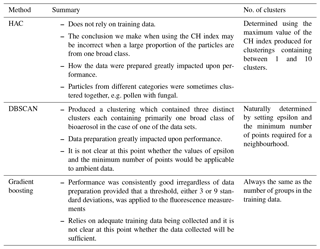
In Sect. 4.1, 4.2, 4.3 we present the results using HAC, DBSCAN and gradient boosting, respectively. A summary of the findings for each method and an indication of how the number of clusters are determined are shown in Table 4.
Table 4Summary of findings and considerations for method selection.
4.1 Hierarchical agglomerative clustering
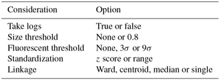
Prior to hierarchical agglomerative clustering (HAC) being applied, we labelled each particle from 1 to 4 to indicate whether the particle was bacteria, fungal, pollen or non-biological, respectively. We then considered a variety of different approaches to prepare the data which are shown in Table 5. Following this, 96 possible combinations of these considerations were applied to the data and the hierarchical agglomerative clustering routine was used to cluster the resultant data in each case. For each of the 96 hierarchies produced, the clusterings containing between 1 and 10 clusters were extracted. Subsequently, a value of the adjusted rand score comparing each of these 10 clusterings to the known labels was calculated. These values of the adjusted rand score would be unavailable during an ambient campaign but are used here to measure the similarity of each clustering to the known labels in order to indicate overall performance and highlight which of the first 10 clusterings was most similar to the known labels. Values of the Calińnski–Harabasz index (CH index), an index which is usually used in an ambient campaign to determine the number of clusters, were also calculated. The number of clusters in the clustering for which the maximum value of the CH index was attained can then be compared to the clustering which is most similar to the known labels to determine if the CH index attains a maximum for the clustering which is most similar to the known labels.
Table 5Outline of the different approaches tested when using hierarchical agglomerative clustering.
4.1.1 Impact of data preparation
Figure 9 provides an overview of the results obtained using the 96 different strategies tested. The data preparation approach suggested in Crawford et al. (2015) (presented in blue) was to take logs of the size and asymmetry factor, use a size threshold of 0.8 µm, use a fluorescent threshold of 3 standard deviations above the average forced-trigger measurement, standardize using the z score and use Ward Linkage. It has also been suggested that a threshold of nine standard deviations may be more appropriate (Savage et al., 2017), so the approach suggested in Crawford et al. (2015) modified to use a threshold of 9σ is also presented (in orange).
In the case of the PSL data set, we see that HAC has produced a clustering with 5 clusters which is very similar to the known labels. The best performance occurred when using a fluorescent threshold of 9 standard deviations, albeit 3 standard deviations produced a similarly high value of the adjusted rand score (0.958).
The maximum adjusted rand scores attained for the laboratory generate aerosol collected in 2008 and 2014 were 0.567 and 0.747. Lower scores are to be expected since we would anticipate laboratory generated aerosol to be more complex than polystyrene latex spheres and hence more difficult to discriminate. The adjusted rand score of the best data strategy of the 96 tested, as indicated by the height of the green bar, is larger than the corresponding adjusted rand score for the strategy suggested in Crawford et al. (2015), indicating that potentially a different strategy may yield better results. However, the best performing strategy was not consistent across both the 2008 and 2014 data.
In particular, the best strategy in 2008 was found to be taking logs; using a size threshold of 0.8 µm; using a fluorescent threshold of 3 standard deviations; standardizing using the range and using Ward linkage. In 2014, the highest value of the adjusted rand score was obtained by not taking logs, not applying a size threshold, using a fluorescent threshold of 9 standard deviations and using the centroid linkage. Since our findings are inconsistent across the two laboratory generated aerosol data sets it becomes difficult to provide a better recommendation for data preparation other than the strategy suggested in Crawford et al. (2015).
In addition, there was a substantial difference between the quality of results attained when using a fluorescent threshold of 3 or 9 standard deviations. In 2008, we see a decrease in the adjusted rand score from 0.482 to 0.277 when using 3 and 9σ, respectively. In 2014, we see an increase in the adjusted rand score from 0.462 to 0.625 when using 3 and 9σ, respectively.
It is possible that the difference in performance when using the different thresholds could be in part explained by the fluorescent threshold in 2014 being constructed using forced trigger data collected at a different time to the laboratory data, or by the fluorescence properties differing across the two data sets. But this differing behaviour when using different data preparation does need to be investigated further with additional laboratory data sets and in the context of ambient data. Nonetheless, the differing conclusions across the two data sets as to which data preparation is preferable does highlight the importance of repeating data collection and demonstrating conclusions are consistent across multiple experiments.
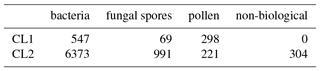
The adjusted rand score is often quite difficult to interpret, so we provide matching matrices for the best and worst case scenario using the current data preparation strategy in Tables 6 and 7. In the best case scenario we are able to discriminate between the pollen and the rest of the data placing 86.8 % of the pollen into Cluster 2. Most of the bacteria is also placed into Cluster 3 with 66.6 % of the fungal spores. A third of the fungal spores are differentiated from the rest of the data and placed into Cluster 1. In the worst case scenario two clusters are provided both primarily containing bacteria. In this case we can conclude that algorithm has failed to differentiate between any of the biological classes, in part due to the CH index concluding there are 2 clusters.

Figure 9Performance of hierarchical agglomerative clustering using the adjusted rand score for the data sets tested across different data preparation strategies. The number of clusters concluded in each case is indicated at the bottom of each bar.
4.1.2 Impact of the Calińnski–Harabasz index
At the base of each bar in Fig. 9 we provided the number of clusters in the clustering for which the adjusted rand score presented was obtained. For the darker bars, this number represents the number of clusters in the clustering for which the highest value of the adjusted rand score was obtained across the clusterings containing between 1 and 10 clusters. For the lighter bars, this number represents the number of the clusters in the clustering for which a maximum of the CH index was attained.
There are three different scenarios that occur. First, the Calińnski–Harabasz index attains a maximum for the clustering which is most similar to the known labels, e.g. for the PSL data using a fluorescent threshold of 3 standard deviations, the clustering which is most similar to the known labels (shown in the darker bar) contains 5 clusters which is the same as the clustering for which a maximum of the CH index is attained (shown in the lighter bar). Second, the Calińnski–Harabasz index attains a maximum for a different clustering than that which is most similar to the known labels, but the conclusion does not have a large impact on performance. For example, in 2008 using a fluorescent threshold of 3 standard deviations, the clustering which is most similar to the known labels contains 5 clusters, whereas the clustering for which the CH index attains a maximum contains 4 clusters. However, the heights of bars are nearly the same. In this case, a very small cluster has been merged in the hierarchy from 5 to 4 clusters resulting in the 4 and 5 cluster clusterings being extremely similar and consequently the fact that the CH index has attained a maximum at 4 clusters instead of 5 is not concerning, since concluding 4 clusters instead of 5 has very little impact upon performance.
The final case is in 2008, using a fluorescent threshold of 9 standard deviations. Here the clustering which is most similar to the known labels is the clustering containing 5 clusters, whereas the CH index attains a maximum for the clustering containing only 2 clusters. The 2 cluster solution in this case is very dissimilar from the known labels.
In the cases where a maximum for the CH index was attained for a clustering containing 2 clusters, i.e. in 2008 using 9σ and in 2014 using 3σ, 78.6 % and 76.5 % of the particles were from a bacterial sample. Conversely in 2008 using 3σ and in 2014 using 9σ, 65.4 % and 68.4 % of the particles analysed were bacteria.
To investigate the possibility of a relationship between the proportion of the data which is contained in the category containing the largest number of particles and the tendency of the CH index to conclude that there are 2 clusters we produced data simulated from 3 normal distributions in 3 dimensions. Each of the clusters was centred around [0, 0, 0], [5, 5, 5], [10, 10, 10] and the co-variance matrix was set to σI3, where I3 is the 3 by 3 identity matrix. The value of σ was varied from 1 to 3 to produce a range of variation in the simulations. We elected to produce this simulated data from normal distributions rather than the laboratory data collected to remove any potential confounding issues such as the fluorescent threshold used. The proportion of the data that was contained in the dominant cluster was varied from 50 % to 99 %. Each simulation was repeated 100 times to provide an indication of the frequency the CH index attains a maximum for the 3 cluster solution.
In Fig. 10 we see that there is a point where the frequency for which the CH index attains a maximum for the clustering containing 3 clusters starts to decrease. The proportion of data points that needs to be placed in the dominant cluster before this decrease in performance of the CH index is seen decreases as the variability in the data increases.
This incorrect conclusion when using the CH index when analysing data for which a large proportion of data are of one particular type is problematic when analysing biological aerosol, since we may expect the quantity of bacteria to be an order of magnitude greater than the fungal spores, and for the quantity of fungal spores to be an order of magnitude greater than the pollen (Després et al., 2012; Gabey, 2011). In future studies it may therefore be necessary to explore the use of other indices for determining the number of clusters.
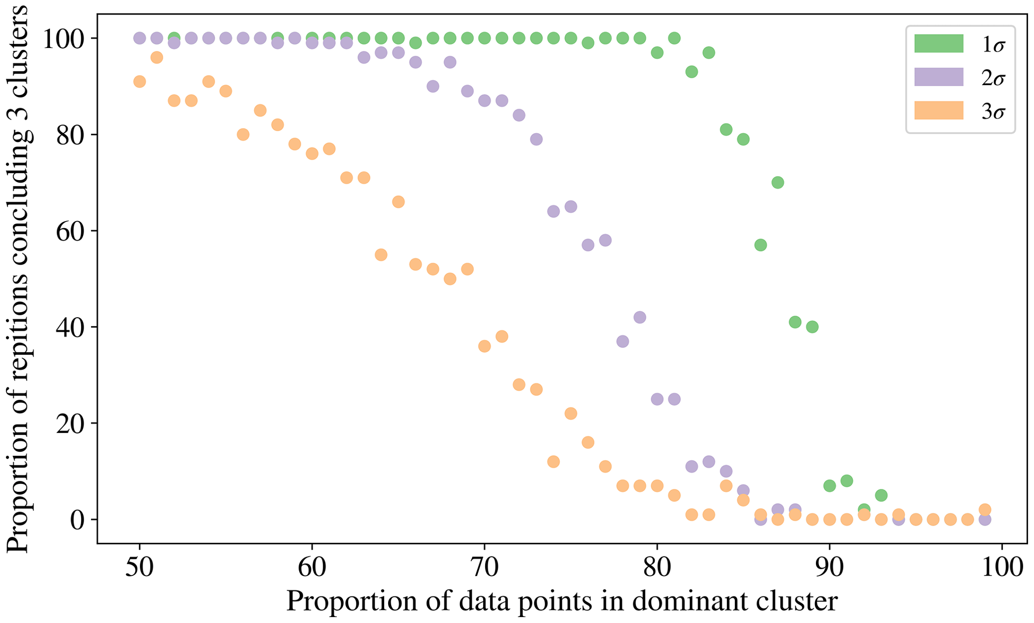
Figure 10Percentage of simulations for which the CH index attained a maximum for the clustering containing 3 clusters against the proportion of the data which is placed into a dominant cluster.
4.1.3 Breakdown of the hierarchies
To more clearly understand how data have been clustered using HAC we have presented dendrograms for the laboratory data collected in 2008 and 2014 in Figs. 11 and 12 alongside heat maps of the matching matrices to indicate the cluster composition of the 10 cluster solution broken down by sample. The hierarchy produced using the strategy suggested in Crawford et al. (2015) is presented at the top of each plot whereas a modification of this strategy using a threshold of 9 standard deviations as suggested by Savage et al. (2017) is presented at the bottom.
Each row of the heat map corresponds to a particular cluster and each column corresponds to a particular sample. The intensity of each box corresponds to the quantity of particles placed into a particular cluster from a particular sample. Bacterial, fungal, pollen and non-biological samples are grouped together in blue, green, orange and black, respectively. Different scales are used for the different groups to prevent the dominant class from obscuring information in the other classes.
In 2008, the majority of the bacteria is placed into a single cluster for both 3σ and 9σ. The fungal and a number of pollen particles are placed into the same two clusters when using 3σ and into one cluster when using 9σ. The non-biological samples, consisting primarily of grass smoke, are clustered mostly with bacterial samples, possibly due to their similar size. In addition, there are two clusters when using 3σ and three clusters when using 9σ containing primarily pollen.
In 2014, pollen has been placed primarily into 1 or 2 clusters. Some of the fungal samples have been placed into a singleton cluster. For both thresholds the bacteria is grouped with some of the fungal samples. The non-biological material has almost entirely been removed by the threshold and the remaining material has been divided among a number of the clusters.
In both 2008 and 2014, some of the material has been segregated into clusters containing primarily one broad class of biological aerosol. However, a number of fungal particles has been grouped with pollen samples in the case of 2008 and a number of the fungal samples have been grouped with bacterial particles in 2014. The more successful segregation of pollen in 2014 may be due to the much larger size range for the paper mulberry sample, whereas in 2008 the fungal and pollen material may be grouped due to presence of a larger number of pollen fragments. It is therefore important when interpreting results from an ambient campaign that it is possible that clusters may contain more than one broad biological class.
Also note that this potentially undesirable grouping of material from two different classes has occurred prior to the final stages of the algorithm and therefore will be apparent in the final solution regardless of the number of clusters concluded, and cannot be rectified by using a different validation index.
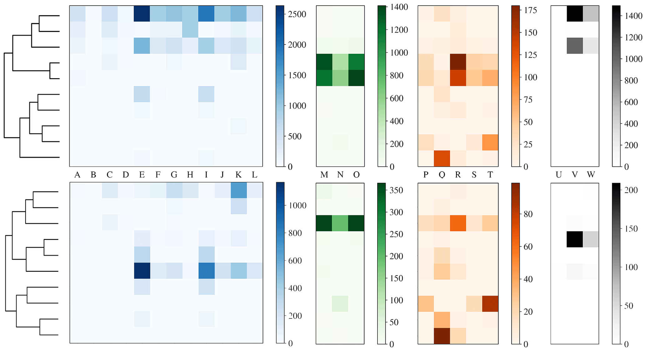
Figure 11Dendrogram truncated at 10 clusters (left) for laboratory data collected in 2008 alongside a heat map of matching matrix (right) indicating cluster composition by each sample segregated by bacteria, fungal, pollen and non-biological in blue, green, orange and black, respectively. Separate scales are used for each broad class to prevent dominant class obscuring detail in the other classes. Hierarchies for 3σ (top) and 9σ (bottom) are presented.

Figure 12Dendrogram truncated at 10 clusters (left) for laboratory data collected in 2014 alongside a heat map of matching matrix (right) indicating cluster composition by each sample segregated by bacteria, fungal, pollen and non-biological in blue, green orange and black, respectively. Separate scales are used for each broad class to prevent the dominant class obscuring detail in the other classes. Hierarchies for 3σ (top) and 9σ (bottom) are presented.
Table 6Matching matrix for the best case scenario when using the current data preparation strategy with 9σ on the data collected in 2014.
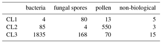
Table 7Matching matrix for the worst case scenario when using the current data preparation strategy with 9σ on the data collected in 2008.
4.2 DBSCAN
One of the main difficulties of using DBSCAN is selecting the minimum number of points to form a neighbourhood and the radius of the neighbourhood (Khan et al., 2014). For 3σ and 9σ using z score standardization, taking logs of the size and asymmetry factor and removing particles smaller than 0.8 µm we repeat the DBSCAN algorithm for a variety of ϵ (neighbourhood radii) and minimum number of points values. The range of values of ϵ we test is 0.1, 0.2, …, 1.0. The range of minimum number of points is set using the following range relative to the number of particles collected 0.1 %, 0.2 %, …, 1.0 %, 2.0 %, …, 10.0 %.
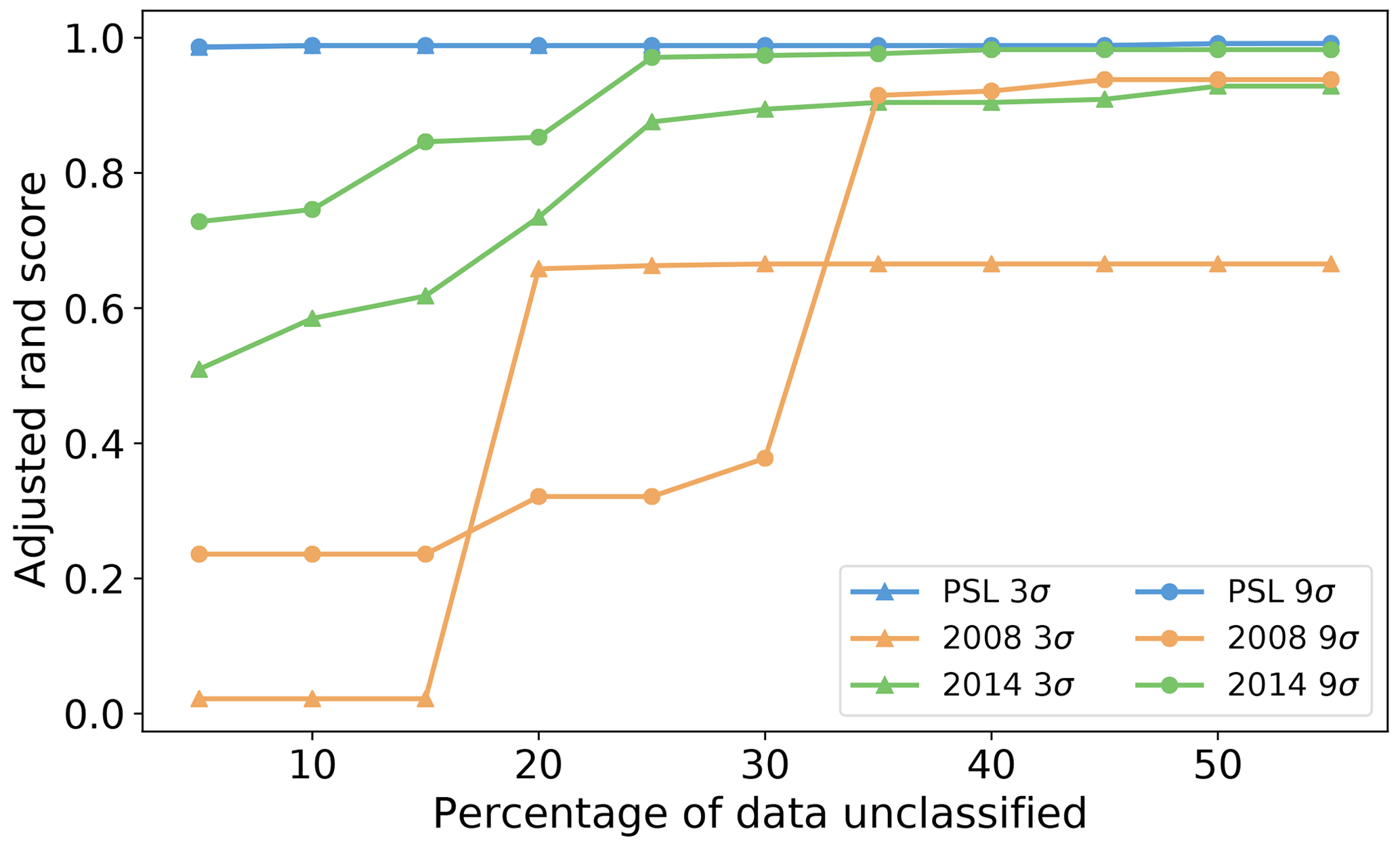
Figure 13Adjusted rand score using different thresholds of percentage of points we allow to be left in the analysis for DBSCAN.
We found wide variety of performance across the different parameters. Often high accuracy could be obtained when using a high value of the minimum number of points but this resulted in removing a substantial portion of the data. In Fig. 13 we filter our results using a range of thresholds for the maximum number of points that can be left unclassified (5 %, 10 %, … 60 %) and plot the corresponding best performance under this filter. In all the data sets there was a point of diminishing returns where no further benefit could be attained by removing any more of the data. In the case of the PSL data, this point happened after removing around 5 % of the particles. For the laboratory data sets between 25 % and 40 % of the data were left unclassified before a peak in performance was attained. Nonetheless, we note in the case of the laboratory data collected in 2014 and using a 9σ fluorescent threshold, we can attain performance similar to that which we attain for the PSL data.
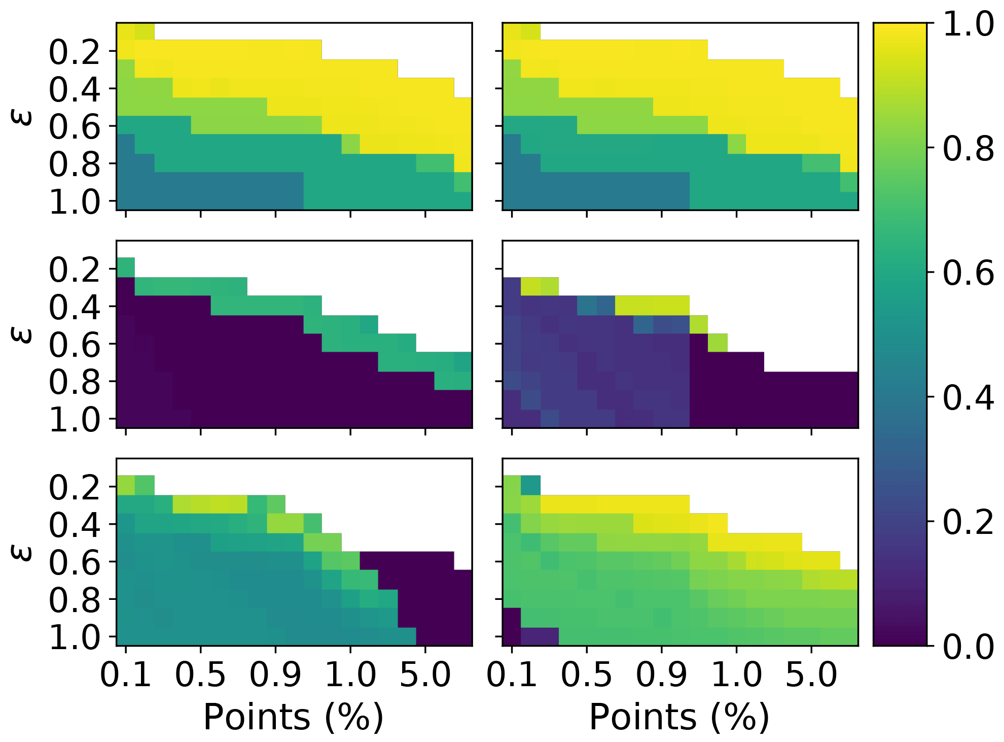
Figure 14Adjusted rand score for DBSCAN, over a range different values of ϵ and minimum number of points required to form a neighbourhood. The minimum number of points is expressed relative to the total number of points. The columns correspond to 3 and 9σ, respectively. The rows correspond to the PSL, 2008 and 2014 data, respectively.
In order to investigate further a choice of ϵ and the minimum number of points which would maximize performance in terms of the adjusted rand score we plot the adjusted rand score for each test across all of the data sets. In Fig. 14 we see that there is a large window of different values for which a higher value of the adjusted rand score can be achieved on the PSLs. Contrary to this, in 2008 when using 9σ there is a very narrow window for which higher values of the adjusted rand score could be attained. It can also be seen that as ϵ increases the number of points required to create a cluster needs to be increased to compensate.
Overall our results indicate setting ϵ=0.3 and ϵ=0.4 when using 3σ and 9σ, respectively. The best results can then be obtained by setting the number of points between 0.4 % and 0.7 % of the data when using an ϵ of 0.3 % and 0.7 % and 1.0 % when using an ϵ of 0.4. However, future research will be required to demonstrate these conclusions are applicable when studying ambient data.
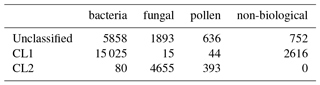
We provide matching matrices for the worst and best case scenarios in Tables 8 and 9. We see that in the best case scenario, leaving a decent proportion of data left unclassified we are able to produce three distinct clusters containing predominantly one broad class of biological aerosol. In the worst case scenario we manage only to distinguish between the bacteria from the fungal spores combined with the pollen.
In the worst case scenario, i.e. using 3σ, on the 2008 data we fail to remove a sizeable fraction of the non-biological particles, which was also the case when using HAC, however we would have expected that the algorithm would leave the particles unclassified. There is some argument that this worst case scenario could be circumvented by simply using the 9σ threshold instead. But further research needs to be conducted on the handling of non-biological material that appears fluorescent in the instrument.
Table 8Matching matrix for the best case scenario when using DBSCAN with 9σ, ϵ=0.4 and a minimum number of points of 0.7 % on the 2014 data.
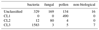
Table 9Matching matrix for the worst case scenario when using DBSCAN with 3σ, ϵ=0.3 and a minimum number of points of 0.4 % on the 2008 data.

4.3 Gradient boosting
We conducted a similar analysis varying data preparation approaches as in Sect. 4.1. We found data preparation to have a very small impact upon performance when using gradient boosting as long as some kind of fluorescence threshold is applied where a high value of the adjusted rand score was obtained regardless of whether we took logs, what standardization was used or the size threshold imposed.
Figure 15 shows the performance using 3σ and 9σ using z score, taking logs and applying a size threshold of 0.8 microns. High performance was attained across both laboratory generated aerosol data sets and for the PSLs. As we did in the previous sections we provide matching matrices of the worst case scenario and best case scenario when using gradient boosting using the current data preparation in Tables 10 and 11. In the best case scenario we provide a very good classification with very small errors (AR=0.933).
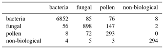
In the worst case scenario a similar performance is achieved (AR=0.882). Nonetheless, a few particles are incorrectly classified within the fungal spore and pollen classes. The classification for the bacteria is still very strong and most of the remaining non-biological particles are correctly classified. The non-biological samples have been removed from this data set prior to gradient boosting being applied when using a fluorescent threshold of either 3σ or 9σ. We elect to remove these particles since too few of the non-biological samples that exceed either threshold to produce a viable training class.
Table 10Matching matrix for the best case scenario when using gradient boosting. This is when using 9σ on the 2014 data.
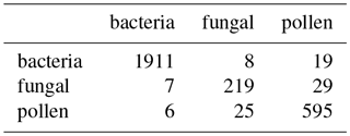
Table 11Matching matrix for the worst case scenario when using gradient boosting. This is when using 9σ on 2008 data.
4.4 K-means
Similar to the findings presented in Ruske et al. (2017), k-means performed poorly and hence the results are omitted from the main text. The results are available in the repository published alongside the paper (see the “Code and data availability” section for further details).
We evaluated a variety of different methods that could be used for classification of biological aerosol. Gradient boosting offered the best performance consistently across the different data preparation strategies and the different data sets tested. That being said it is unclear at this point how this will translate to ambient data and whether or not the training data currently collected will be sufficient to outline the variety of environments that could potentially be studied.
Should there not be sufficient training data available an unsupervised approach may be required. In this case, a possible alternative to HAC is provided. In the best case scenario DBSCAN, despite leaving a decent proportion of the data unclassified, was able to produce three distinct clusters containing predominantly one biological class each.
To the best of our knowledge this is the first paper using DBSCAN to classify biological aerosol using the WIBS. So we will need to continue to evaluate the performance of this algorithm in the context of the ambient setting. In particular, we have provided details of what we believe to be sensible selections of epsilon and the minimum number of points on the basis of the laboratory data collected. However, it is unclear at this point how effective these selections will be when analysing ambient data.
When applied the laboratory generated aerosol tested, we found that performance of HAC was in general much lower than what was achieved previously using the PSLs (Crawford et al., 2015). Performance was heavily dependent on the data preparation strategy used, and often results could vary substantially between different strategies and data sets, potentially due to differences in the fluorescence measurements across the two data sets. A potential issue with the CH index is highlighted, whereby we see a failure of the index to determine the correct number of clusters as the size of the dominant class and variation in the data increases. Some of the pollen samples were clustered with the fungal samples when analysing the data from 2008. A number of the pollen particles may be fragmented which may explain why this grouping may occur. Similarly grass smoke was grouped with the bacterial samples, potentially due to their similar size. Caution will therefore be required when applying the HAC algorithm to ambient data, and it must be noted in particular that material from two different classes may be placed into the same cluster and that the CH index may indicate an incorrect number of clusters if the data collected contains a significant quantity of one particular type of particle.
In the future, more laboratory generated aerosol particles will need to be collected to continue to evaluate the performance of the algorithms which we use. In addition, when gradient boosting was used we failed to classify the some of the pollen and fungal spore samples analysed. It is therefore possible that higher spectral instruments such as the spectral intensity bioaerosol sensor (Nasir et al., 2018), will be required to provide a more accurate classification.
Part of the code used produce the above paper is part of an ongoing development of a software suite for analysis of various UV-LIF instruments, available at https://github.com/simonruske/UVLIF, last access: 5 November 2018, upon publication, and Ruske (2018a). Other code not currently included within the software package, i.e. code files which are used to produce the plots and figures specific to the current paper are available at https://github.com/simonruske/AMT-2018-126, last access: 13 November 2018, and Ruske (2018b).
The data used is available upon request by contacting the lead author.
Table A1Average particle sizes for the current study compared with other studies. The sizes presented here are collated from the following studies [1] Healy et al. (2012a), [2] Savage et al. (2017), [3] Hernandez et al. (2016), [4] Pierucci (1978), [5] Carrera et al. (2007), [6] Crotzer and Levetin (1996), [7] Geiser et al. (2000), [8] Pinnick et al. (1995), [9] Fumanal et al. (2007), [10] Mäkelä (1996), [11] Kang et al. (2007), [2008] and [2014] are taken from the current study.
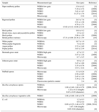
To contextualize the samples collected in the current study we examined the literature to find similar studies using the WIBS as well as other studies using microscopy. In the case of most of the samples we were able to find a paper on the same or similar species of particle which are presented in Table A1.
Table B1For the data collected in 2008, a summary of size and fluorescent measurements for each sample to include: the number of particles in the sample (total), average equivalent optical diameter (EOD), standard deviation of the size (σ), the number of points that exceeded a fluorescent threshold of 3 standard deviations above the average forced trigger measurement (n>3σ), and ABC counts using a 3σ threshold.
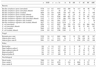
Table B2For the data collected in 2014, a summary of size and fluorescent measurements for each sample to include: the number of particles in the sample (total), average equivalent optical diameter (EOD), standard deviation of the size (σ), the number of points that exceeded a fluorescent threshold of 3 standard deviations above the average forced trigger measurement (n>3σ), and ABC counts using a 3σ threshold.
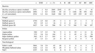
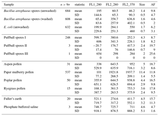
Table B3Summary of properties for samples collected from 2008 and 2014, respectively, using a fluorescent threshold of 9σ.
To aid in comparing the data presented with other studies, we have presented Tables B1 and B2 which are very similar to the table in the appendices of Hernandez et al. (2016). A, B and C are used to denote particles which exceed the fluorescent threshold in FL1_280, FL2_280, FL2_370, respectively. For example A is used to denote a particle that was only fluorescent in the FL1_280 channel only. Combinations such as AB, AC, BC and ABC are used to denote particles which exceed a fluorescent threshold in more than one channel. For example, AB is used to denote a particle that exceeded the fluorescent in both the FL1_280 and FL2_280 channels.
The same information but using a 9σ threshold instead is presented in Table B3.
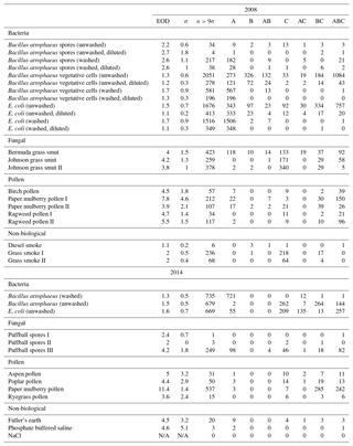
Table C1Summary of particle measurements for the 2008 data set using a fluorescent threshold of 3σ.
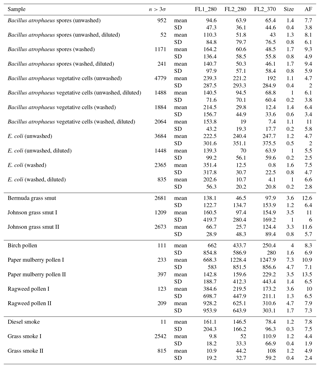
Table C2Summary of particle measurements for the 2008 data set using a fluorescent threshold of 9σ.
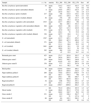
Table C3Summary of particle measurements for the 2014 data set using a fluorescent threshold of 3σ.
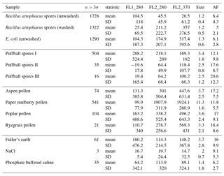
Table C4Summary of particle measurements for the 2014 data set using a fluorescent threshold of 9σ.
In the following section we summarize mean and standard deviations in each of the five measurements in each of the samples collected in 2008 and 2014. The properties presented in Tables C1, C2, C3 and C4 are after a size threshold of 0.8 µm is imposed and a fluorescent threshold of either 3σ or 9σ has been applied. These summary statistics presented are prior to any log-transformations or data standardization has been applied.
Collection of the laboratory generated aerosol samples in 2008 and 2014 was undertaken at the Defence, Science and Technology Laboratory for which the primary point of contact was VEF who provided substantial assistance in writing and editing the data section. SR conducted analysis of the derived data products and produced the figures and tables assisted by DOT and MWG. SR took the lead on writing the manuscript with discussion and critical feedback from all authors throughout the drafting and publication process.
The authors declare that they have no conflict of interest.
Simon Ruske is funded by NERC (NERC grant no. NE/L002469/1) and the University of Manchester.
Edited by: Mingjin Tang
Reviewed by: Darrel Baumgardner and one anonymous referee
Breiman, L.: Bagging predictors, Machine Learning, 24, 123–140, 1996. a
Breiman, L.: Random forests, Machine Learning, 45, 5–32, 2001. a
Caliński, T. and Harabasz, J.: A dendrite method for cluster analysis, Commun. Stat. A-Theor., 3, 1–27, 1974. a, b
Carrera, M., Zandomeni, R., Fitzgibbon, J., and Sagripanti, J.-L.: Difference between the spore sizes of Bacillus anthracis and other Bacillus species, J. Appl. Microbiol., 102, 303–312, 2007. a
Crawford, I., Bower, K. N., Choularton, T. W., Dearden, C., Crosier, J., Westbrook, C., Capes, G., Coe, H., Connolly, P. J., Dorsey, J. R., Gallagher, M. W., Williams, P., Trembath, J., Cui, Z., and Blyth, A.: Ice formation and development in aged, wintertime cumulus over the UK: observations and modelling, Atmos. Chem. Phys., 12, 4963–4985, https://doi.org/10.5194/acp-12-4963-2012, 2012. a
Crawford, I., Ruske, S., Topping, D. O., and Gallagher, M. W.: Evaluation of hierarchical agglomerative cluster analysis methods for discrimination of primary biological aerosol, Atmos. Meas. Tech., 8, 4979–4991, https://doi.org/10.5194/amt-8-4979-2015, 2015. a, b, c, d, e, f, g, h, i, j, k
Crawford, I., Gallagher, M. W., Bower, K. N., Choularton, T. W., Flynn, M. J., Ruske, S., Listowski, C., Brough, N., Lachlan-Cope, T., Fleming, Z. L., Foot, V. E., and Stanley, W. R.: Real-time detection of airborne fluorescent bioparticles in Antarctica, Atmos. Chem. Phys., 17, 14291–14307, https://doi.org/10.5194/acp-17-14291-2017, 2017. a
Crotzer, V. and Levetin, E.: The aerobiological significance of smut spores in Tulsa, Oklahoma, Aerobiologia, 12, 177–184, 1996. a
Cziczo, D. J., Froyd, K. D., Hoose, C., Jensen, E. J., Diao, M., Zondlo, M. A., Smith, J. B., Twohy, C. H., and Murphy, D. M.: Clarifying the dominant sources and mechanisms of cirrus cloud formation, Science, 340, 1320–1324, 2013. a
D'Amato, G., Liccardi, G., D'amato, M., and Cazzola, M.: The role of outdoor air pollution and climatic changes on the rising trends in respiratory allergy, Resp. Med., 95, 606–611, 2001. a
Després, V. R., Huffman, J. A., Burrows, S. M., Hoose, C., Safatov, A. S., Buryak, G. A., Fröhlich-Nowoisky, J., Elbert, W., Andreae, M. O., Pöschl, U., and Jaenicke, R.: Primary Biological Aerosol Particles in the Atmosphere: A Review, Tellus B, 64, 15598, https://doi.org/10.3402/tellusb.v64i0.15598, 2012. a, b
Freund, Y. and Schapire, R. E.: A decision-theoretic generalization of on-line learning and an application to boosting, J. Comput. Syst. Sci., 55, 119–139, 1997. a
Friedman, J., Hastie, T., and Tibshirani, R.: The elements of statistical learning, vol. 1, Springer series in statistics New York, NY, USA, 2001. a
Friedman, J. H.: Greedy function approximation: a gradient boosting machine, Ann. Stat., 29, 1189–1232, 2001. a
Fumanal, B., Chauvel, B., and Bretagnolle, F.: Estimation of pollen and seed production of common ragweed in France, Ann. Agr. Env. Med., 14, 233–236, 2007. a
Gabey, A. M.: Laboratory and field characterisation of fluorescent and primary biological aerosol particles, PhD thesis, The University of Manchester, Manchester, UK, 2011. a, b
Gabey, A. M., Gallagher, M. W., Whitehead, J., Dorsey, J. R., Kaye, P. H., and Stanley, W. R.: Measurements and comparison of primary biological aerosol above and below a tropical forest canopy using a dual channel fluorescence spectrometer, Atmos. Chem. Phys., 10, 4453–4466, https://doi.org/10.5194/acp-10-4453-2010, 2010. a, b
Gabey, A. M., Stanley, W. R., Gallagher, M. W., and Kaye, P. H.: The fluorescence properties of aerosol larger than 0.8 µm in urban and tropical rainforest locations, Atmos. Chem. Phys., 11, 5491–5504, https://doi.org/10.5194/acp-11-5491-2011, 2011. a
Gabey, A. M., Gallagher, M. W., Whitehead, J., Dorsey, J. R., Kaye, P. H., and Stanley, W. R.: Measurements and comparison of primary biological aerosol above and below a tropical forest canopy using a dual channel fluorescence spectrometer, Atmos. Chem. Phys., 10, 4453–4466, https://doi.org/10.5194/acp-10-4453-2010, 2010. a
Geiser, M., Leupin, N., Maye, I., Im Hof, V., and Gehr, P.: Interaction of fungal spores with the lungs: distribution and retention of inhaled puffball (Calvatia excipuliformis) spores, J. Allergy Clin. Immun., 106, 92–100, 2000. a
Gurian-Sherman, D. and Lindow, S. E.: Bacterial ice nucleation: significance and molecular basis., The FASEB journal, 7, 1338–1343, 1993. a
Hader, J. D., Wright, T. P., and Petters, M. D.: Contribution of pollen to atmospheric ice nuclei concentrations, Atmos. Chem. Phys., 14, 5433–5449, https://doi.org/10.5194/acp-14-5433-2014, 2014. a
Healy, D. A., O'Connor, D. J., Burke, A. M., and Sodeau, J. R.: A laboratory assessment of the Waveband Integrated Bioaerosol Sensor (WIBS-4) using individual samples of pollen and fungal spore material, Atmos. Environ., 60, 534–543, 2012a. a, b, c
Healy, D. A., O'Connor, D. J., and Sodeau, J. R.: Measurement of the particle counting efficiency of the “Waveband Integrated Bioaerosol Sensor” model number 4 (WIBS-4), J. Aerosol Sci., 47, 94–99, 2012b. a
Hernandez, M., Perring, A. E., McCabe, K., Kok, G., Granger, G., and Baumgardner, D.: Chamber catalogues of optical and fluorescent signatures distinguish bioaerosol classes, Atmos. Meas. Tech., 9, 3283–3292, https://doi.org/10.5194/amt-9-3283-2016, 2016. a, b, c, d
Hoose, C. and Möhler, O.: Heterogeneous ice nucleation on atmospheric aerosols: a review of results from laboratory experiments, Atmos. Chem. Phys., 12, 9817–9854, https://doi.org/10.5194/acp-12-9817-2012, 2012. a
Hubert, L. and Arabie, P.: Comparing partitions, J. Classif., 2, 193–218, 1985. a
Kang, D.-Y., Son, M.-S., Eum, C.-H., Kim, W.-S., and Lee, S.-H.: Size determination of pollens using gravitational and sedimentation field-flow fractionation, B. Kor. Chem. Soc., 28, 613–618, 2007. a
Kaye, P. H., Stanley, W., Hirst, E., Foot, E., Baxter, K., and Barrington, S.: Single particle multichannel bio-aerosol fluorescence sensor, Opt. Express, 13, 3583–3593, 2005. a, b
Kennedy, R. and Smith, M.: Effects of aeroallergens on human health under climate change, in: Health Effects of Climate Change in the UK 2012, edited by: Vardoulakis, S. and Heaviside, C., 83–96, 2012. a
Khan, K., Rehman, S. U., Aziz, K., Fong, S., and Sarasvady, S.: DBSCAN: Past, present and future, in: Applications of Digital Information and Web Technologies (ICADIWT), 2014 Fifth International Conference on the IEEE, 232–238, 2014. a
Mäkelä, E. M.: Size distinctions between Betula pollen types – a review, Grana, 35, 248–256, 1996. a
Milligan, G. W. and Cooper, M. C.: An examination of procedures for determining the number of clusters in a data set, Psychometrika, 50, 159–179, 1985. a
Milligan, G. W. and Cooper, M. C.: A study of standardization of variables in cluster analysis, J. Classif., 5, 181–204, 1988. a
Möhler, O., DeMott, P. J., Vali, G., and Levin, Z.: Microbiology and atmospheric processes: the role of biological particles in cloud physics, Biogeosciences, 4, 1059–1071, https://doi.org/10.5194/bg-4-1059-2007, 2007. a
Müllner, D.: Modern hierarchical, agglomerative clustering algorithms, arXiv preprint arXiv:1109.2378, 2011. a
Müllner, D.: fastcluster: Fast hierarchical, agglomerative clustering routines for R and Python, J. Stat. Softw., 53, 1–18, 2013. a, b
Nasir, Z., Rolph, C., Collins, S., Stevenson, D., Gladding, T., Hayes, E., Williams, B., Khera, S., Jackson, S., Bennett, A., Parks, S., Kinnersley, R. P., Walsh, K., Pollard, S. J. T., Drew, G., Garcia-Alcega, S., Coulon, F., and Tyrrel, S.: A Controlled Study on the Characterisation of Bioaerosols Emissions from Compost, Atmosphere, 9, 379, https://doi.org/10.3390/atmos9100379, 2018. a
Pedregosa, F., Varoquaux, G., Gramfort, A., Michel, V., Thirion, B., Grisel, O., Blondel, M., Prettenhofer, P., Weiss, R., Dubourg, V., Vanderplas, J., Passos, A., Cournapeau, D., Brucher, M., Perrot, M., and Duchesnay, E.: Scikit-learn: Machine Learning in Python, J. Mach. Learn. Res., 12, 2825–2830, 2011. a, b
Pierucci, O.: Dimensions of Escherichia coli at various growth rates: model for envelope growth, J. Bacteriol., 135, 559–574, 1978. a
Pinnick, R. G., Hill, S. C., Nachman, P., Pendleton, J. D., Fernandez, G. L., Mayo, M. W., and Bruno, J. G.: Fluorescence particle counter for detecting airborne bacteria and other biological particles, Aerosol Sci. Tech., 23, 653–664, 1995. a
Pöhlker, C., Huffman, J. A., and Pöschl, U.: Autofluorescence of atmospheric bioaerosols – fluorescent biomolecules and potential interferences, Atmos. Meas. Tech., 5, 37–71, https://doi.org/10.5194/amt-5-37-2012, 2012. a
Pöhlker, C., Huffman, J. A., Förster, J.-D., and Pöschl, U.: Autofluorescence of atmospheric bioaerosols: spectral fingerprints and taxonomic trends of pollen, Atmos. Meas. Tech., 6, 3369–3392, https://doi.org/10.5194/amt-6-3369-2013, 2013. a
Robinson, N. H., Allan, J. D., Huffman, J. A., Kaye, P. H., Foot, V. E., and Gallagher, M.: Cluster analysis of WIBS single-particle bioaerosol data, Atmos. Meas. Tech., 6, 337–347, https://doi.org/10.5194/amt-6-337-2013, 2013. a, b
Ruske, S.: simonruske/UVLIF: Pre-release of software (Version 0.0.1), Zenodo, https://doi.org/10.5281/zenodo.1478098, 5 November 2018a.
Ruske, S.: simonruske/AMT-2018-126: Code release upon acceptance (Version 1.0.0), Zenodo, https://doi.org/10.5281/zenodo.1478082, 5 November 2018b.
Ruske, S., Topping, D. O., Foot, V. E., Kaye, P. H., Stanley, W. R., Crawford, I., Morse, A. P., and Gallagher, M. W.: Evaluation of machine learning algorithms for classification of primary biological aerosol using a new UV-LIF spectrometer, Atmos. Meas. Tech., 10, 695–708, https://doi.org/10.5194/amt-10-695-2017, 2017. a, b, c, d
Savage, N. J. and Huffman, J. A.: Evaluation of a hierarchical agglomerative clustering method applied to WIBS laboratory data for improved discrimination of biological particles by comparing data preparation techniques, Atmos. Meas. Tech., 11, 4929–4942, https://doi.org/10.5194/amt-11-4929-2018, 2018. a
Savage, N. J., Krentz, C. E., Könemann, T., Han, T. T., Mainelis, G., Pöhlker, C., and Huffman, J. A.: Systematic characterization and fluorescence threshold strategies for the wideband integrated bioaerosol sensor (WIBS) using size-resolved biological and interfering particles, Atmos. Meas. Tech., 10, 4279–4302, https://doi.org/10.5194/amt-10-4279-2017, 2017. a, b, c, d, e, f
Schubert, E., Koos, A., Emrich, T., Züfle, A., Schmid, K. A., and Zimek, A.: A Framework for Clustering Uncertain Data, Proceedings of the VLDB Endowment, 8, 1976–1979, available at: http://www.vldb.org/pvldb/vol8/p1976-schubert.pdf (last access: 20 February 2018), 2015. a
Ting, K. M.: Confusion Matrix, pp. 209–209, Springer US, Boston, MA, https://doi.org/10.1007/978-0-387-30164-8_157, 2010. a
Vinh, N. X., Epps, J., and Bailey, J.: Information theoretic measures for clusterings comparison: Variants, properties, normalization and correction for chance, J. Mach. Learn. Res., 11, 2837–2854, 2010. a
- Abstract
- Introduction
- Methods
- Data
- Results
- Conclusions
- Code and data availability
- Appendix A: Comparison of particle size with other studies
- Appendix B: ABC counts and average particle sizes
- Appendix C: Summary of average properties of the different data sets
- Author contributions
- Competing interests
- Acknowledgements
- References