the Creative Commons Attribution 4.0 License.
the Creative Commons Attribution 4.0 License.
 | 21 Nov 2018
Stratosphere–troposphere separation of nitrogen dioxide columns from the TEMPO geostationary satellite instrument
Randall V. Martin
Eric J. Bucsela
Chris A. McLinden
Daniel J. M. Cunningham
Separating the stratospheric and tropospheric contributions in satellite retrievals of atmospheric NO2 column abundance is a crucial step in the interpretation and application of the satellite observations. A variety of stratosphere–troposphere separation algorithms have been developed for sun-synchronous instruments in low Earth orbit (LEO) that benefit from global coverage, including broad clean regions with negligible tropospheric NO2 compared to stratospheric NO2. These global sun-synchronous algorithms need to be evaluated and refined for forthcoming geostationary instruments focused on continental regions, which lack this global context and require hourly estimates of the stratospheric column. Here we develop and assess a spatial filtering algorithm for the upcoming TEMPO geostationary instrument that will target North America. Developments include using independent satellite observations to identify likely locations of tropospheric enhancements, using independent LEO observations for spatial context, consideration of diurnally varying partial fields of regard, and a filter based on stratospheric to tropospheric air mass factor ratios. We test the algorithm with LEO observations from the OMI instrument with an afternoon overpass, and from the GOME-2 instrument with a morning overpass.
We compare our TEMPO field of regard algorithm against an identical global algorithm to investigate the penalty resulting from the limited spatial coverage in geostationary orbit, and find excellent agreement in the estimated mean daily tropospheric NO2 column densities (R2=0.999, slope=1.009 for July and R2=0.998, slope=0.999 for January). The algorithm performs well even when only small parts of the continent are observed by TEMPO. The algorithm is challenged the most by east coast morning retrievals in the wintertime (e.g., R2=0.995, slope=1.038 at 14:00 UTC). We find independent global LEO observations (corrected for time of day) provide important context near the field-of-regard edges. We also test the performance of the TEMPO algorithm without these supporting global observations. Most of the continent is unaffected (R2=0.924 and slope=0.973 for July and R2=0.996 and slope=1.008 for January), with 90 % of the pixels having differences of less than molecules cm−2 between the TEMPO tropospheric NO2 column density and the global algorithm. For near-real-time retrieval, even a climatological estimate of the stratospheric NO2 surrounding the field of regard would improve this agreement. In general, the additional penalty of a limited field of regard from TEMPO introduces no more error than normally expected in most global stratosphere–troposphere separation algorithms. Overall, we conclude that hourly near-real-time stratosphere–troposphere separation for the retrieval of NO2 tropospheric column densities by the TEMPO geostationary instrument is both feasible and robust, regardless of the diurnally varying limited field of regard.


Nitrogen dioxide (NO2) and nitrogen oxides in general are central to atmospheric chemistry in both the troposphere and stratosphere (Finlayson-Pitts and Pitts, 1999; Seinfeld and Pandis, 2016). In the stratosphere, nitrogen oxides are a key player in ozone (O3) depletion chemistry. In the troposphere, photolysis of NO2 is responsible for the production of O3 whose buildup is associated with negative human health, ecosystem, and radiative forcing impacts. Emissions of nitrogen oxides are also linked to the production of secondary inorganic aerosol with impacts on both health and global climate. Observations of NO2 in the atmosphere are therefore critical given its roles in air quality and atmospheric chemistry.
Satellite remote sensing of NO2 from instruments in low Earth orbit (LEO) has offered extraordinary insight into global nitrogen oxide processes. Among many applications, observations from GOME (1996–2003), SCIAMACHY (2002–2011), OMI (2004–), and GOME-2 (2007–) have contributed to understanding global and regional patterns in nitrogen oxide emissions (e.g., Beirle et al., 2003; Duncan et al., 2013; Jaegle et al., 2005; Konovalov et al., 2008; Lamsal et al., 2011; Martin et al., 2003; Miyazaki et al., 2017; Richter et al., 2005; Russell et al., 2012), evaluating ground-level air quality in the absence of traditional monitoring data (e.g., Bechle et al., 2013; Boersma et al., 2009; Geddes et al., 2016; Lamsal et al., 2008; McLinden et al., 2012), and constraining nitrogen oxide deposition out of the atmosphere (e.g., Geddes and Martin, 2017; Jia et al., 2016; Nowlan et al., 2014). A key step in these applications is the separation of stratospheric and tropospheric NO2 from the total column derived from the satellite observation, a process that can introduce substantial uncertainty the final tropospheric column estimates (Beirle et al., 2016; Boersma et al., 2004; Bucsela et al., 2013; Martin et al., 2002).
Separating the stratospheric and tropospheric contributions to the total column has been performed using a number of approaches, varying in complexity and in the assumptions that are made. The simplest approach is the Pacific reference sector method (Beirle et al., 2003; Martin et al., 2002; Richter and Burrows, 2002) in which stratospheric NO2 is treated as longitudinally homogeneous so that stratospheric NO2 in any location can be estimated by using the measured NO2 over the remote Pacific at the same latitude. Tropospheric NO2 in the reference sector might either be ignored altogether (e.g., Richter and Burrows, 2002) or accounted for using a model estimate (e.g., Martin et al., 2002). While the treatment of zonal invariance is reasonable for low- to mid-latitudes, stratospheric dynamics (especially in the vicinity of polar vortices) raise concerns at higher latitudes of relevance for planned geostationary missions.
Image processing and spatial filtering techniques are an extension of the reference sector method (Bucsela et al., 2006, 2013; Leue et al., 2001; Valks et al., 2011; Velders et al., 2001; Wenig et al., 2004), whereby stratospheric NO2 is estimated by interpolating between regions that are classified as having negligible tropospheric NO2. This might be accomplished for example by using only cloudy scenes over the oceans (e.g., Leue et al., 2001), or by applying a pollution “mask” given prior estimates of tropospheric NO2 (e.g., Bucsela et al., 2006; Valks et al., 2011). Bucsela et al. (2013) proposed a masking scheme that combines a prior estimate of tropospheric NO2 with radiative transfer calculations to allow polluted pixels to remain if the scene is cloudy (obscuring lower tropospheric NO2), and exclude unpolluted regions where tropospheric NO2 signal may still be significant due to high tropospheric air mass factors. An elegant variation of this spatial filtering approach is the STRatospheric Estimation Algorithm from Mainz (STREAM), developed by Beirle et al. (2016). Instead of binary masks based on arbitrary thresholds, STREAM applies a weighted convolution scheme where cloudy observations are given a high weight and polluted observations (based on a prior estimate) are given low weight. These spatial filtering approaches developed exclusively for global observational coverage from LEO offer valuable guidance on the development of geostationary stratosphere–troposphere separation algorithms.
Nadir observations are also used in assimilation approaches where model predictions of the stratospheric NO2 column density are adjusted towards the observed column density. For example, stratosphere–troposphere separation in the Dutch NO2 algorithm is achieved by assimilating observed NO2 columns with model NO2 column predictions from the TM4 chemical transport model forced by European Centre for Medium-Range Weather Forecasts (ECMWF) meteorological data (Boersma et al., 2007; Dirksen et al., 2011). In that approach, modeled NO2 profiles are convolved into line-of-sight (“slant”) columns using averaging kernels, and the difference between modeled and observed slant column densities are used to force the modeled columns to an “analyzed” state. Using the most recent observations available, the “analyzed” state can be used in a forecast model run to predict the stratospheric field for near-real time retrievals (Boersma et al., 2007).
In some cases, independent stratospheric observations may be used in the separation of stratospheric and tropospheric NO2. For example, the SCIAMACHY instrument made almost coincident nadir and limb measurements (Bovensmann et al., 1999) and this matching was exploited in algorithms by Beirle et al. (2010) and Hilboll et al. (2013). Even non-coincident limb–nadir matching has been exploited for stratosphere–troposphere separation, as in the case of OSIRIS and OMI (Adams et al., 2016). Sussmann et al. (2005) demonstrate how simultaneous ground-based measurements (especially at mountain sites) could be applied for stratosphere–troposphere separation algorithm validation.
To date, all of the above approaches to stratosphere–troposphere separation have been developed using the large coverage of observations provided by instruments in LEO. Questions remain about how well the separation can be performed without the global context and where clean tropospheric background signals are limited. Stratosphere–troposphere separation algorithms need to be evaluated and refined for the restricted field of regard of future geostationary instruments such as TEMPO (Zoogman et al., 2017), Sentinel-4 (Courrege-Lacoste et al., 2017), and GEMS (Lasnik et al., 2014).
TEMPO (“Tropospheric Emissions: Monitoring of Pollution”), launching between 2019–2021, will provide space-based measurements in geostationary orbit with a field of regard over North America from southern Canada to Mexico City and the Bahamas (Zoogman et al., 2017). The spectrometer has spectral ranges of 290–490 nm (at 0.57 nm resolution) and 540–740 nm (at 0.2 nm resolution), allowing retrieval of tropospheric composition with fine spatial resolution (up to 2.1 km north–south×4.4 km east–west instantaneous field of view). Scanning occurs from east to west, with hourly revisits. Among its standard products available at roughly 4 km×8 km spatial resolution will be hourly NO2 column abundance. Here, we develop a standard stratosphere–troposphere separation algorithm for the observations of NO2 from TEMPO, and examine in detail the potential information penalty associated with the limited TEMPO field of regard compared to an identical global algorithm.
To develop and test our algorithm, we use data from two LEO instruments, with afternoon and morning overpasses. We use NO2 column densities derived from OMI on board the Aura satellite launched in 2004. OMI is a nadir-viewing spectrometer in LEO crossing the equator around 13:30 local time, with a variable horizontal resolution of 13 km×24 km at nadir. Line-of-slight (“slant”) columns are retrieved from spectral fitting of back-scattered and reflected solar radiation within the 405–465 nm wavelength range, and corrected for instrumental artifacts (Bucsela et al., 2013). We use the Version 3.0 Standard Product NO2 retrieval (SPv3) from NASA (Krotkov et al., 2017, publicly available at https://disc.gsfc.nasa.gov/datasets/OMNO2_V003/summary, last access: 9 November 2018), including stratospheric and tropospheric air mass factors provided with the data to relate slant and vertical columns (Bucsela et al., 2013). We use the artifact-corrected slant column densities (“destriping”) and the tropospheric and stratospheric air mass factors calculated for each pixel. All data are first gridded to a regular grid.
We also make use of NO2 column densities derived from GOME-2, on board the MetOp-A satellite launched in 2006. GOME-2 is another nadir-viewing spectrometer in LEO, crossing the equator around 09:30 local time with a constant horizontal resolution of 80 km×40 km in its default swath. Spectral fitting is performed within the 420–450 nm wavelength range. Here we use the TM4NO2A retrieval (Boersma et al., 2004) version 2.3 data product from KNMI (available from http://www.temis.nl/airpollution/no2.html, last access: 9 November 2018) along with the included air mass factors.
We restrict all data to solar zenith angles smaller than 80∘ to avoid exceedingly long path lengths.
Here we describe our approach to estimate the stratospheric NO2 column in TEMPO observations. As a foundation for our method, we begin with the approach used in the current operational algorithm for OMI (Bucsela et al., 2013). This algorithm has demonstrated high quality performance against validation data sets (Ialongo et al., 2016; Lamsal et al., 2014; Bucsela et al., 2013), is computationally fast, and is suitable for near-real-time retrievals. Our own implementation of this algorithm reproduces the operational global stratospheric NO2 product well (r=0.99 and a slope of 1.01). As described below, we build on this algorithm for TEMPO by modifying certain smoothing and filtering steps, using a satellite-derived prior estimate of tropospheric NO2, incorporating observations surrounding the TEMPO field of regard from independent LEO instruments, and by considering partial fields of regard relevant to TEMPO.
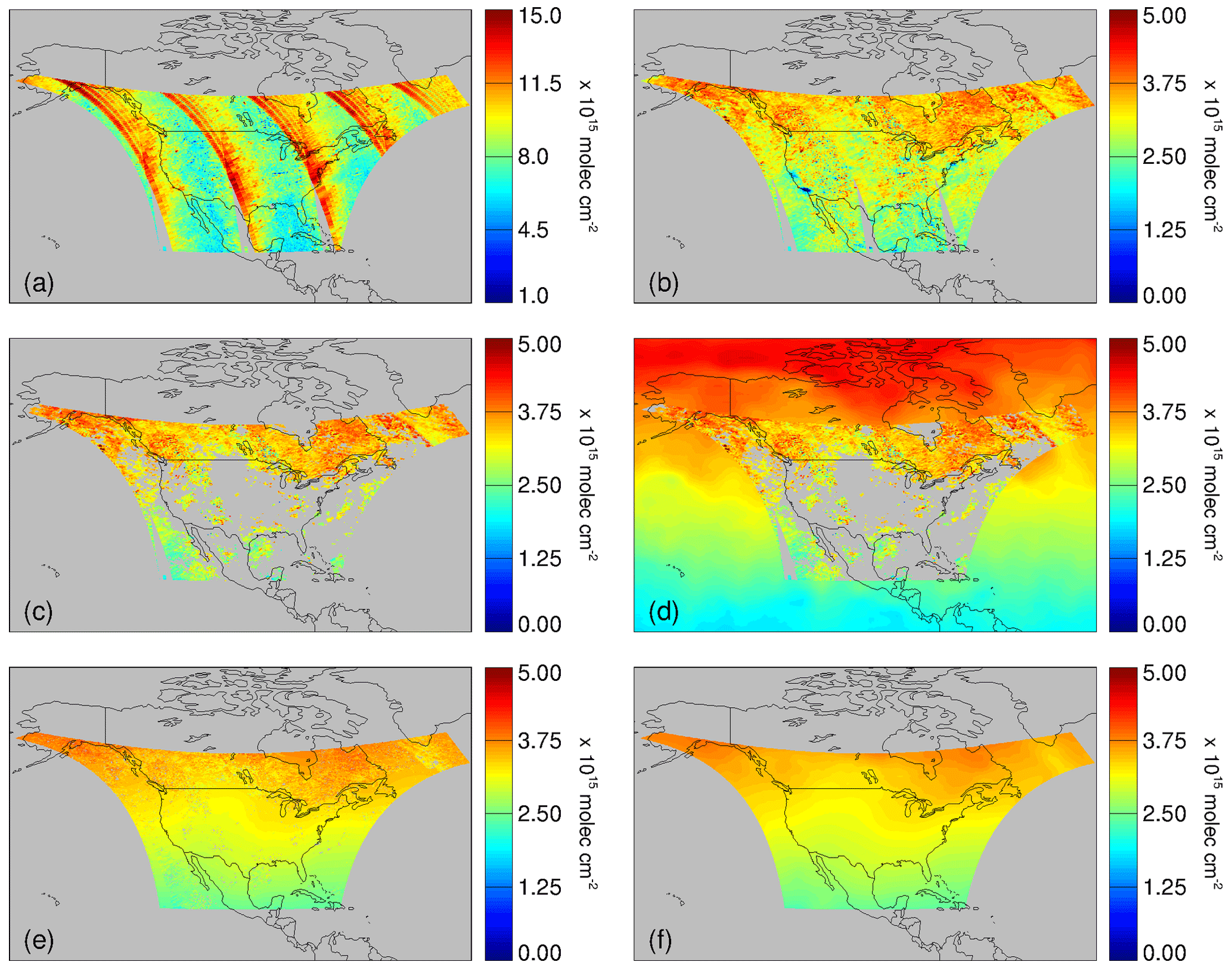
Figure 1Calculation of the stratospheric NO2 estimate on 15 July 2007, using OMI observations from within the anticipated TEMPO field of regard: (a) slant columns on a grid. (b) Initial stratospheric estimate (Vinit) resulting from Eqs. (1) and (2). (c) Masked Vinit using a threshold of molecules cm−2 to remove large tropospheric influence. (d) Adding context outside of the TEMPO field of regard by using independent low-Earth-orbit observations from GOME-2 that have been corrected for time of day. (e) Stratospheric NO2 estimate with masked areas interpolated. (f) Stratospheric NO2 estimate after final hot spot removal and smoothing.
Figure 1 shows the stepwise implementation of our TEMPO stratosphere–troposphere separation algorithm for an example day in July. As a surrogate for TEMPO observations, we begin by restricting the OMI total slant NO2 column observations to the anticipated TEMPO field of regard below a solar zenith angle threshold of 80∘ (Fig. 1a). The expected coverage of TEMPO extends from as far south as Mexico City, northward to include southern Canada (covering as far north as the oil sands region in Alberta for example). The pattern along the orbit tracks in Fig. 1a results from the changing OMI viewing zenith angle (with higher slant columns for larger viewing angles). Although we begin our implementation with the OMI observations gridded to , the TEMPO algorithm would be performed on the individual TEMPO pixels. In other words, here we are treating our gridded OMI observations as TEMPO pixels.
An initial estimate of the stratospheric vertical NO2 column (Vinit) can be obtained by
where S is the total slant column density, Astrat is the stratospheric air mass factor, and Strop,prior accounts for small contributions from the troposphere (Bucsela et al., 2013). Bucsela et al. (2013) estimated the tropospheric contribution using model values. To provide a more accurate constraint on tropospheric contributions, we use the monthly mean tropospheric NO2 columns derived from independent GOME-2 observations as an initial a priori tropospheric NO2 estimate. The GOME-2 observations were filtered using recommended quality flags and retaining pixels with cloud radiance fraction less than 0.5, then gridded to the same resolution as our OMI grid. This concept enables the use of spatial information observed from satellite, and could be readily adapted to use TROPOMI observations at finer resolution. Ideally, an independent LEO tropospheric estimate for as close to the TEMPO observation time would be used. Nonetheless, diurnal variability in tropospheric NO2 columns outside of source regions tends to be small (Boersma et al., 2008), and in our case source regions are masked out in a later step. The use of a satellite-derived a priori reduces the use of chemical transport model information in the stratosphere–troposphere separation algorithm (although we revert to a model estimate if quality controlled satellite coverage is not available, e.g., due to systematically high cloud fractions). We transform this satellite-derived a priori tropospheric NO2 vertical column (Vtrop,prior) into slant column space using the tropospheric air mass factors (Atrop) provided with the OMI data:
Figure 1b shows our initial estimate of stratospheric vertical NO2 columns over the TEMPO domain resulting from the combination of Eqs. (1) and (2). We already see that this stratospheric NO2 estimate varies predominately as a function of latitude, although anomalously low values are seen over some urban centers (e.g., around Los Angeles, Chicago, and New York) where the a priori tropospheric NO2 slant column is large.
To exclude locations where this initial stratospheric vertical column estimate is likely biased, we make use of the masking approach from Bucsela et al. (2013). This is based on eliminating pixels where tropospheric contamination is high (or where the initial stratospheric vertical column estimate would exceed the actual stratospheric vertical column by some reasonable value) by requiring:
On a typical day in July, this means that contamination from the troposphere would be less than ∼10 % percent of the stratospheric NO2 estimate (which generally ranges from 2–4×1015 cm−2 over the TEMPO field of regard). Figure 1c shows the result of this masking step. The threshold removes all the urban regions with anomalously low values in Fig. 1b, in addition to many other areas. Sensitivity tests show that the final stratospheric NO2 estimate varies by less than 5 % for changes in this threshold between 0.2×10¹⁵ or 0.4×1015 cm−2, consistent with the generally small sensitivity found by Bucsela et al. (2013). On this example day (and for the month of July on average) the masking threshold of 0.3×1015 cm−2 removes 55 % of the original data within the TEMPO field of regard. We find coverage is best over Canada and over the Pacific Ocean, with less coverage over the rest of the continent and the Atlantic Ocean. The original global algorithm removes ∼28 % of the available global data on average for days in July, since tropospheric NO2 columns are generally lower elsewhere in the world.
Since Strop,prior is calculated based on radiative transfer calculations (Atrop) in addition to the a priori tropospheric NO2 vertical column (Eq. 2), this masking approach in principle allows for polluted pixels to remain if the lower tropospheric signal is sufficiently suppressed by clouds resulting in a low tropospheric air mass factor (or conversely excludes pixels with a considerable tropospheric signal due to high surface reflectivity). We investigated the use of explicitly cloudy scenes (cloud radiance fraction >0.9), which could suppress the signal from below. Mid-level clouds (600–400 hPa) are the least likely to contain significant NOx mixed in from the surface, or lightning NOx associated with higher clouds. We find that most (>75 %) of the pixels that meet these criteria are already retained by our original masking algorithm. Incorporating the remaining cloudy pixels to the masked data increases data coverage by less than 1 %. Given the uncertainties in retrieving cloud properties, uncertainties in cloudy air mass factors, and the minimal added value of this dataset, we disregard adding the remaining cloudy pixels to our algorithm.
In Bucsela et al. (2013), the remaining unmasked data are binned and un-filled bins are interpolated using 2-dimensional averaging with a latitude moving window. In our case, this step necessarily precludes information from outside the TEMPO field of regard over the mostly pristine oceans from being used in the 2-D averaging. As we will show, this leads to biases near the field of regard edges when compared to a global algorithm, since the averaging window is disproportionately impacted by observations with continental influence. We reduce this bias by incorporating independent global observations from LEO that can provide context outside of the TEMPO field of regard. This approach exploits the independent LEO observations that are expected throughout the lifespan of TEMPO (e.g., GOME-2, TROPOMI).
Here, we employ GOME-2 observations as an independent dataset to estimate stratospheric NO2 at GOME-2 overpass time outside the TEMPO field of regard by using an identical algorithm on this global data. We empirically transform the GOME-2 stratospheric NO2 estimate to the TEMPO observation time (here, the OMI overpass time), using the climatological 30-day running mean local ratio of GOME-2 to OMI stratospheric NO2. A similar observational or model climatology could readily be constructed with TEMPO data after launch based on the available LEO observations at the time. Figure 1d shows the outcome of this approach. The GOME-2 observations outside of the TEMPO field of regard retain the same magnitude and latitudinal gradient as the available observations within the TEMPO field of regard, suggesting that the additional context from an independent LEO instrument can be useful even when they are from a different time of day.
Before interpolating the unfilled bins, we apply a boxcar filter using a moving window as follows. First, our boxcar filter returns a smoothed array using the following algorithm:
where
where w is the smoothing width (in our case, defined in two dimensions by both a length and width), Ri is the ith point in the smoothed data, and Ai is the ith point in the original data. For data points where the neighborhood includes points outside the array, the nearest edge points are used to compute the smoothed result. The variance of the original data is also calculated using a similar algorithm. Any value that lies outside of the moving window average by ±1.5 standard deviations is removed. While the Bucsela et al. (2013) algorithm uses the same window size in a boxcar filtering step, it is performed later and only remove values above the mean (“hotspots”). Here, we perform this boxcar filter in both directions (above and below the mean) to remove anomalously low values that might result from a biased a priori tropospheric estimate that was not accounted for in the masking step (avoiding negative stratospheric NO2 values being retained in subsequent steps), and to remove anomalously high values that might result from transient pollution events that were likewise missed in the masking step. We perform this boxcar filter twice to strictly remove outliers from regions with noisy data.
Missing bins are then interpolated using a latitude moving window. We tested smaller window sizes and found that they could introduce unphysical variability, and/or leave missing data. Figure 1e shows how all the missing data over the TEMPO domain are successfully filled using this window size. A few remaining “hot spots” are accounted for in a third pass of the boxcar filter.
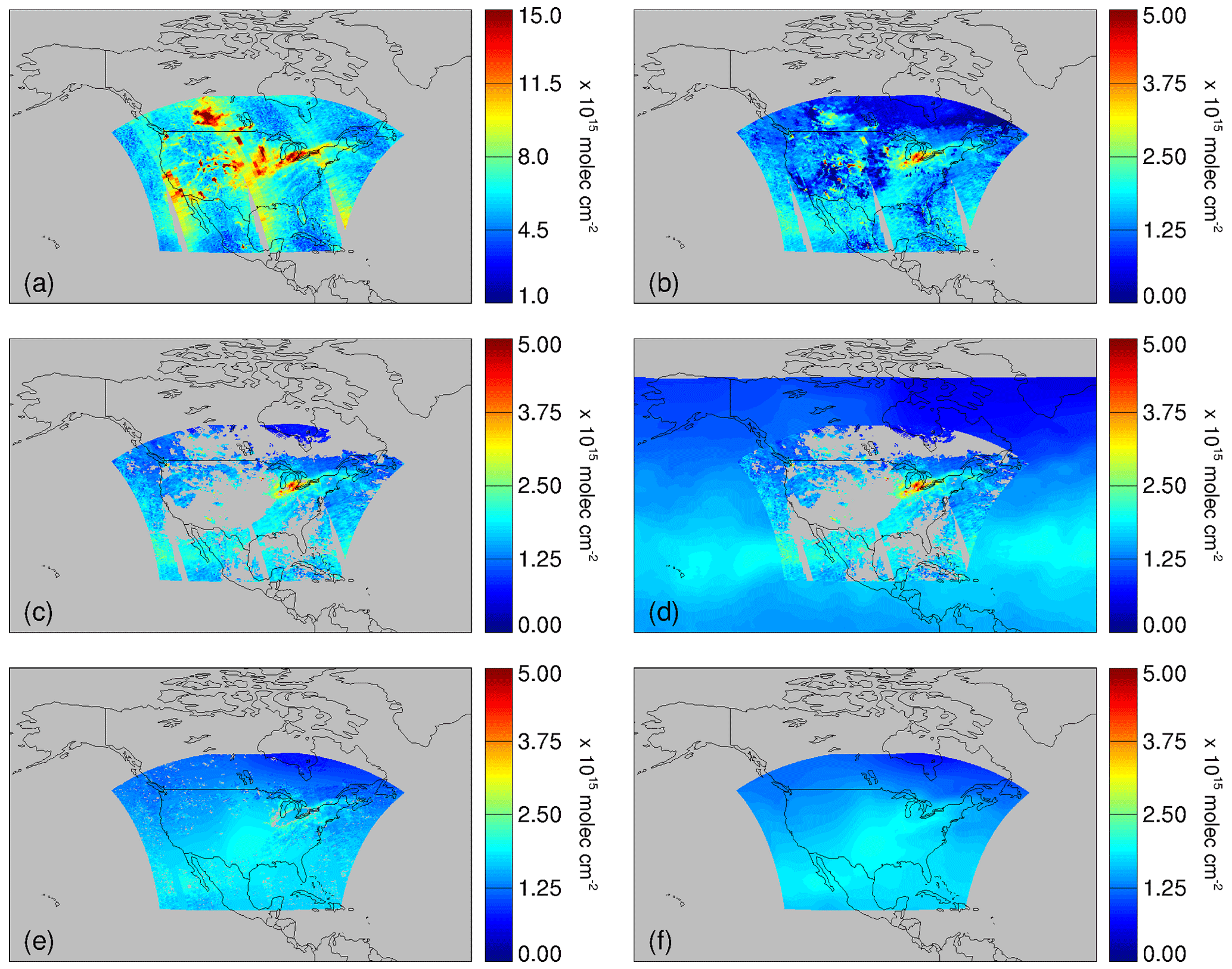
Figure 2Calculation of the stratospheric NO2 estimate on 15 January 2007, using OMI observations from within the anticipated TEMPO field of regard: (a) slant columns on a grid. (b) Initial stratospheric estimate (Vinit) resulting from Eqs. (1) and (2). (c) Masked Vinit using a threshold of molecules cm−2 to remove large tropospheric influence. (d) Adding context outside of the TEMPO field of regard by using independent low-Earth-orbit observations from GOME-2 that have been corrected for time of day. (e) Stratospheric NO2 estimate with masked areas interpolated. (f) Stratospheric NO2 estimate after final hot spot removal and smoothing.
To obtain our final stratospheric NO2 column estimate, we apply a final simple smoothing step with a window, as in Bucsela et al. (2013). The smaller box-car window size in this step recognizes, and allows for, some regional scale variability in the stratosphere. Figure 1f shows the final stratospheric NO2 column estimate over the TEMPO field of regard. Variation is primarily a function of latitude, from around 2×10¹⁵ molecules cm−2 at the lowest latitudes in the field of regard ( latitude) to around 4×10¹⁵ molecules cm−2 at the highest latitudes ( latitude). It is also apparent that this spatial filtering algorithm allows for important regional scale variability to be retained in the stratospheric estimate.
In an effort to evaluate our new TEMPO algorithm with an independent estimate, we compare our stratospheric vertical column with the stratospheric vertical column included in the OMI SPv3 retrieval. Despite using different prior tropospheric estimates, incorporating observations from GOME-2 outside the field of regard during interpolation, and employing different box-car filtering steps, our algorithm is highly consistent with the results from the global NASA standard OMI product over the TEMPO field of regard (r=0.972, m=0.986). Overall, we calculate a mean bias in our new TEMPO algorithm compared to the NASA standard product of only molecules cm−2 (a normalized mean bias of −1.5 %).
Figure 2 shows the results of the same algorithm from an example day in January. The shape of the expected TEMPO domain is impacted by large solar zenith angles at the highest latitudes (we again use a solar zenith angle cut-off of 80∘). Tropospheric enhancements feature more prominently in the total slant column (Fig. 2a) than in July since stratospheric NO2 columns are lower in the winter, and tropospheric NO2 columns are higher. Figure 2b shows the initial stratospheric estimate (Vinit) from Eq. (1), again using the monthly mean GOME-2 tropospheric NO2 column as an a priori estimate (Eq. 2). Figure 2c shows the result of applying the masking threshold (Eq. 3). We find this threshold removes 51 % of the available data on average for this month (∼21 % of the available data are removed in the global algorithm in January). Over the TEMPO domain we find that a slightly smaller fraction pixels are removed in January compared to July because, despite having generally higher NO2 tropospheric column densities, tropospheric air mass factors across the northeast are extremely low at this time of year (discussed below). The low values are primarily due to increased wintertime cloudiness. In this case, the masking threshold did not remove a strong enhancement over the center of the continent. This highlights some criticism by Beirle et al. (2016) of spatial filtering algorithms that rely strongly on a priori climatologies wherein transient tropospheric events could be misinterpreted as stratospheric. We find that varying the magnitude of the threshold (Eq. 3) does not successfully correct for this, since our masking approach is based on a monthly mean and does not identify transient events, but this feature is diminished in subsequent steps. Figure 2d shows the estimated stratospheric NO2 outside of the TEMPO field of regard from the independent GOME-2 observations. Again, these LEO observations provide powerful context despite being from a different time of day. Figure 2e shows the result of the first two passes of the boxcar filter, and interpolating unfilled bins using the latitude moving window.
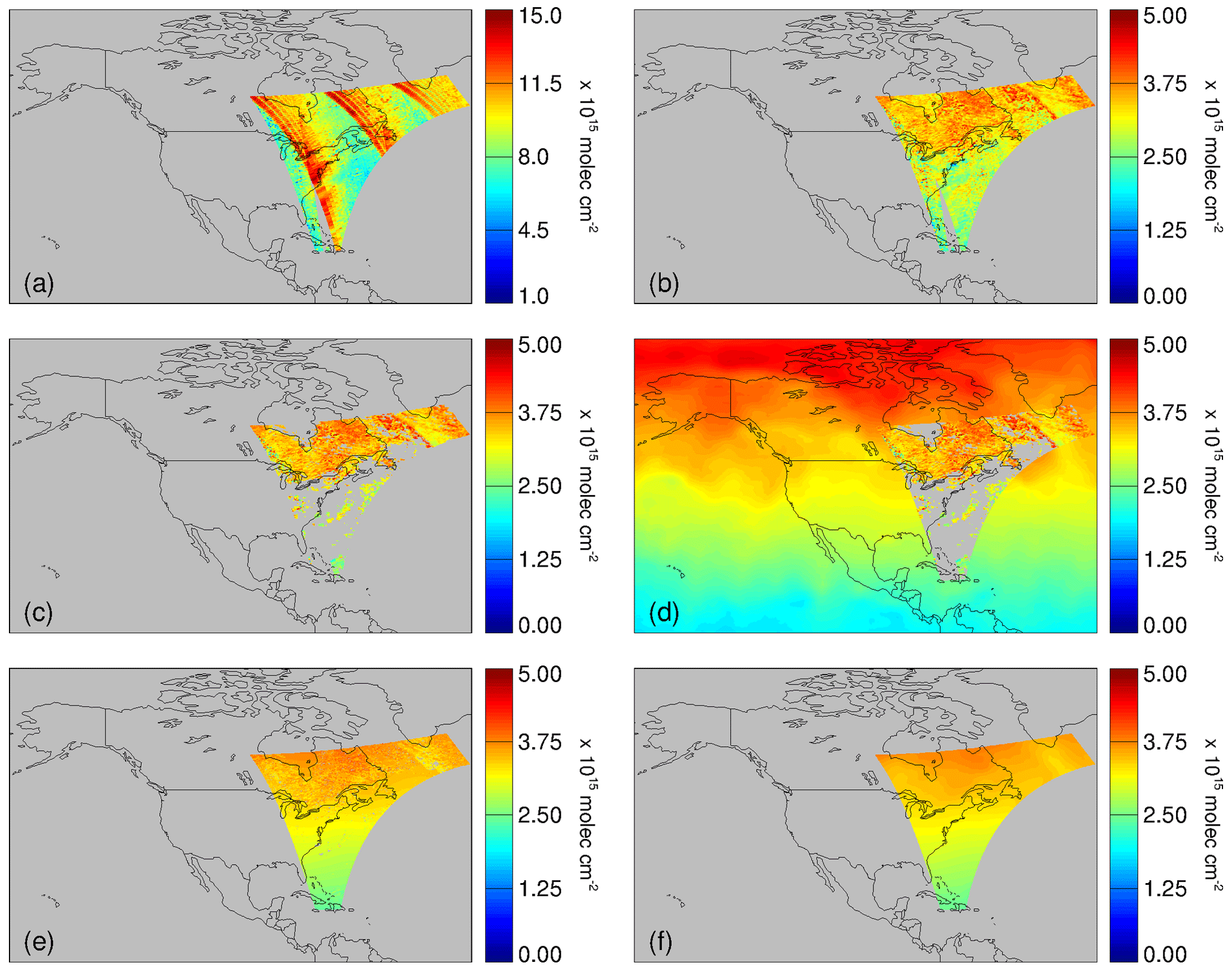
Figure 3Calculation of the stratospheric NO2 estimate on 15 July 2007, using OMI observations from within the anticipated TEMPO field of regard at 11:30 UTC (06:30 Eastern Standard Time): (a) slant columns on a grid. (b) Initial stratospheric estimate (Vinit) resulting from Eqs. (1) and (2). (c) Masked Vinit using a threshold of molecules cm−2 to remove large tropospheric influence. (d) Adding context outside of the TEMPO field of regard by using independent low-Earth-orbit observations from GOME-2 that have been corrected for time of day. (e) Stratospheric NO2 estimate with masked areas interpolated and smoothed. (f) Stratospheric NO2 estimate after final hot spot removal smoothing.
Figure 2f shows the final stratospheric NO2 estimate after the final pass of the statistical test and smoothing. The large enhancement of NO2 over the continent has been substantially dampened by our statistical filtering. The variability in the stratospheric NO2 column is again generally latitudinal as expected, with values above 2×10¹⁵ molecules cm−2 at the low latitudes, and below 1×10¹⁵ molecules cm−2 at the high latitudes.
The full TEMPO domain will have simultaneous sunlit coverage from about 14:00 to 23:00 UTC in July, and for only a few hours in January, based on a solar zenith angle threshold of . Of concern is the lack of coverage over the west coast in the morning, and over the east coast in the evening, where sunlit observations will not be available. Under these circumstances, the stratospheric separation algorithm is challenged by even narrower spatial domains. We evaluate these cases by repeating the calculations at specific times of day.
Figure 3 shows how the TEMPO algorithm would operate for 11:30 Coordinated Universal Time (UTC), 06:30 Eastern Standard Time (EST), on the example day in July. Daylight observations over eastern North America are available by this time, without coverage over the rest of the continent. All the algorithm steps are identical to those in Figs. 1 and 2 other than treatment of this partial coverage (additional near-real-time considerations are discussed in Sect. 5). Figure 3a shows the OMI total slant columns. By 06:30 EST TEMPO observes only eastern North America. The availability of observations increases in width northward because of the TEMPO viewing geometry. Figure 3b and c show the initial stratospheric estimate (according to Eq. 1) and the masked stratospheric estimate (according to Eq. 3) respectively. Figure 3d shows the independent LEO observations from GOME-2 outside of the TEMPO field of regard. The observations are binned, pass the statistical filtering steps, and interpolated in Fig. 3e. The final stratospheric estimate is shown in Fig. 3f. Comparing this final stratospheric NO2 estimate with the estimate in Fig. 1f (where coverage over the whole continent is assumed to be available), we see the reduced coverage has negligible impact the final stratospheric estimate, and identical spatial features are preserved (R2=0.995).
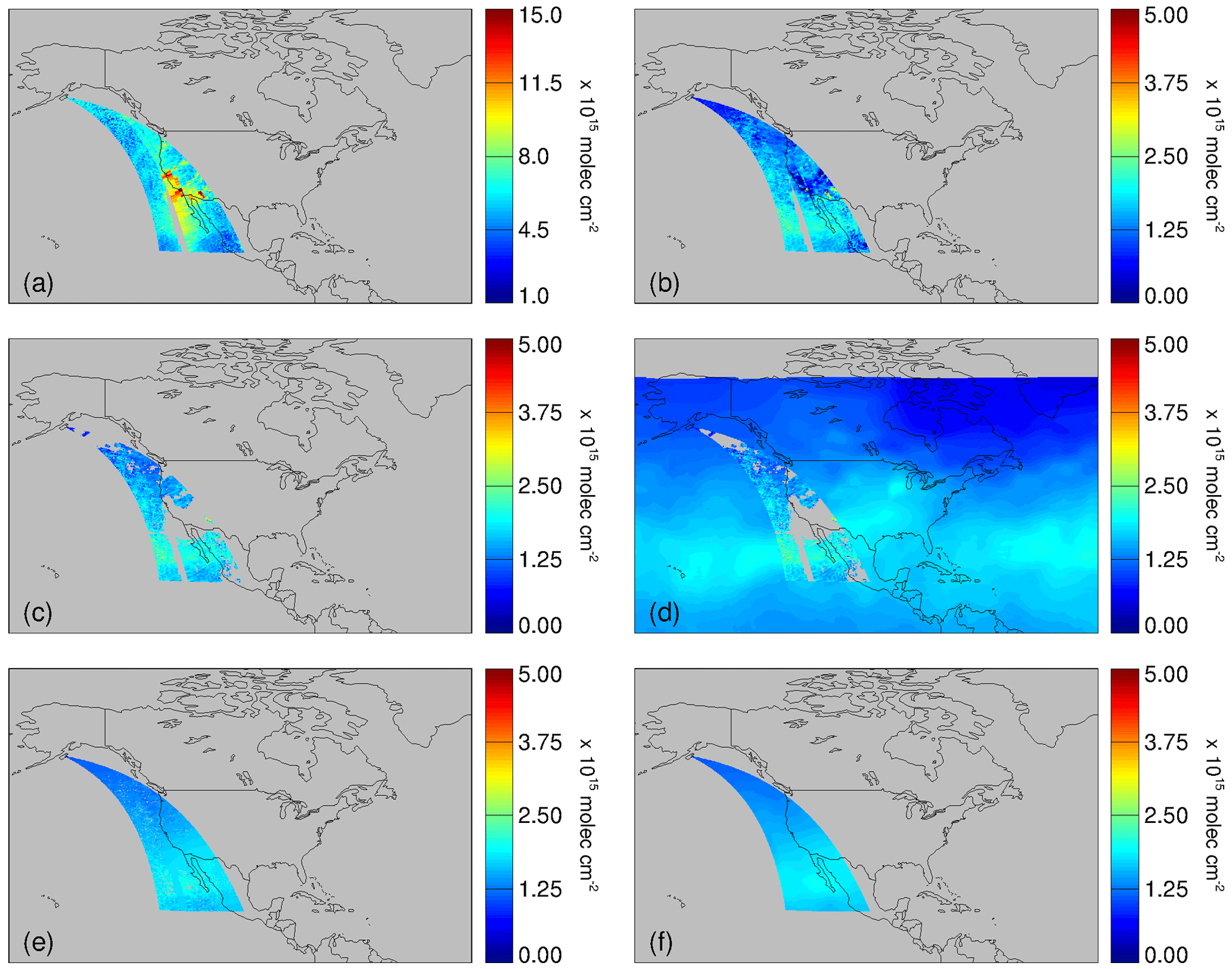
Figure 4Calculation of the stratospheric NO2 estimate on 15 January 2007, using OMI observations from within the anticipated TEMPO field of regard at 23:30 UTC (15:30 Pacific Standard Time): (a) slant columns at resolution. (b) Initial stratospheric estimate (Vinit) resulting from Eq. (2). (c) Masked Vinit using a threshold of molecules cm−2 to remove large tropospheric influence. (d) Adding context outside of the available TEMPO field of regard by using independent low-Earth-orbit observations from GOME-2 that have been corrected for time of day. (e) Stratospheric NO2 estimate with masked areas interpolated and smoothed. (f) Final stratospheric NO2 estimate after hot spot removal and smoothing.
Likewise, Fig. 4 shows how the algorithm would operate on the example day in January at 23:30 UTC, or 15:30 Pacific Standard Time (PST). In addition to the loss of observations in the east due to the time of day, larger solar zenith angles in the north at this time of year further diminish coverage. Again, the subsequent steps are otherwise identical to those in Figs. 1 through 3. Figure 4a shows the OMI total slant columns. Observations are available over parts of the Pacific Northwest, with coverage widening southward so that observations are available from California to the western edge of Texas, and over western parts of Mexico. Figure 4b and c show the initial stratospheric estimate (according to Eq. 1) and the masked stratospheric estimate (according to Eq. 3) respectively. Figure 4d shows how the independent LEO observations from again GOME-2 provide coverage outside of the TEMPO field of regard. After binning and interpolation (Fig. 4e) followed by hot spot removal and smoothing, the final TEMPO stratospheric estimate is shown in Fig. 4f. Comparing this stratospheric NO2 estimate with Fig. 2f (where coverage over the whole continent is assumed to be available) demonstrates again how the reduced coverage has negligible impact the final stratospheric estimate, and identical spatial features are preserved (R2=0.997).
Next, we examine in detail the potential information penalty associated with the limited TEMPO field of regard compared to a global implementation of our algorithm, and demonstrate quantitatively that our approach can produce a tropospheric NO2 estimate that is consistent with a global algorithm, regardless of the time of day.
The final step in the algorithm is the subtraction of the stratospheric NO2 estimate from the total slant column to obtain the tropospheric NO2 column by
For this calculation we use the stratospheric and tropospheric air mass factors provided with the OMI data product (the operational TEMPO algorithm would use TEMPO air mass factors).
The difference between two tropospheric NO2 column retrievals (Vtrop,2 and Vtrop,1) that result from two different stratospheric NO2 estimates (Vstrat,2 and Vstrat,1), but identical slant columns and air mass factors, is directly proportional to the ratio of the tropospheric to stratospheric air mass factors:
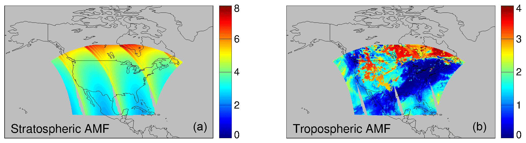
This means that differences (or errors) in stratospheric NO2 estimates are magnified in the tropospheric NO2 column depending on the local air mass factors. This issue is particularly important over the eastern US in the winter, where tropospheric air mass factors can be very low (<0.1), and stratospheric air mass factors can be high (∼5) depending on viewing geometry. Figure 5 shows the stratospheric and tropospheric air mass factors for 15 January 2007. Over areas of the eastern US, where clouds prevail, the tropospheric air mass factors are exceedingly small (∼0.01), which gives rise to extremely large Astrat∕Atrop ratios (>200). In other words, residuals between two stratospheric NO2 algorithms can become magnified by more than two orders of magnitude in the troposphere.
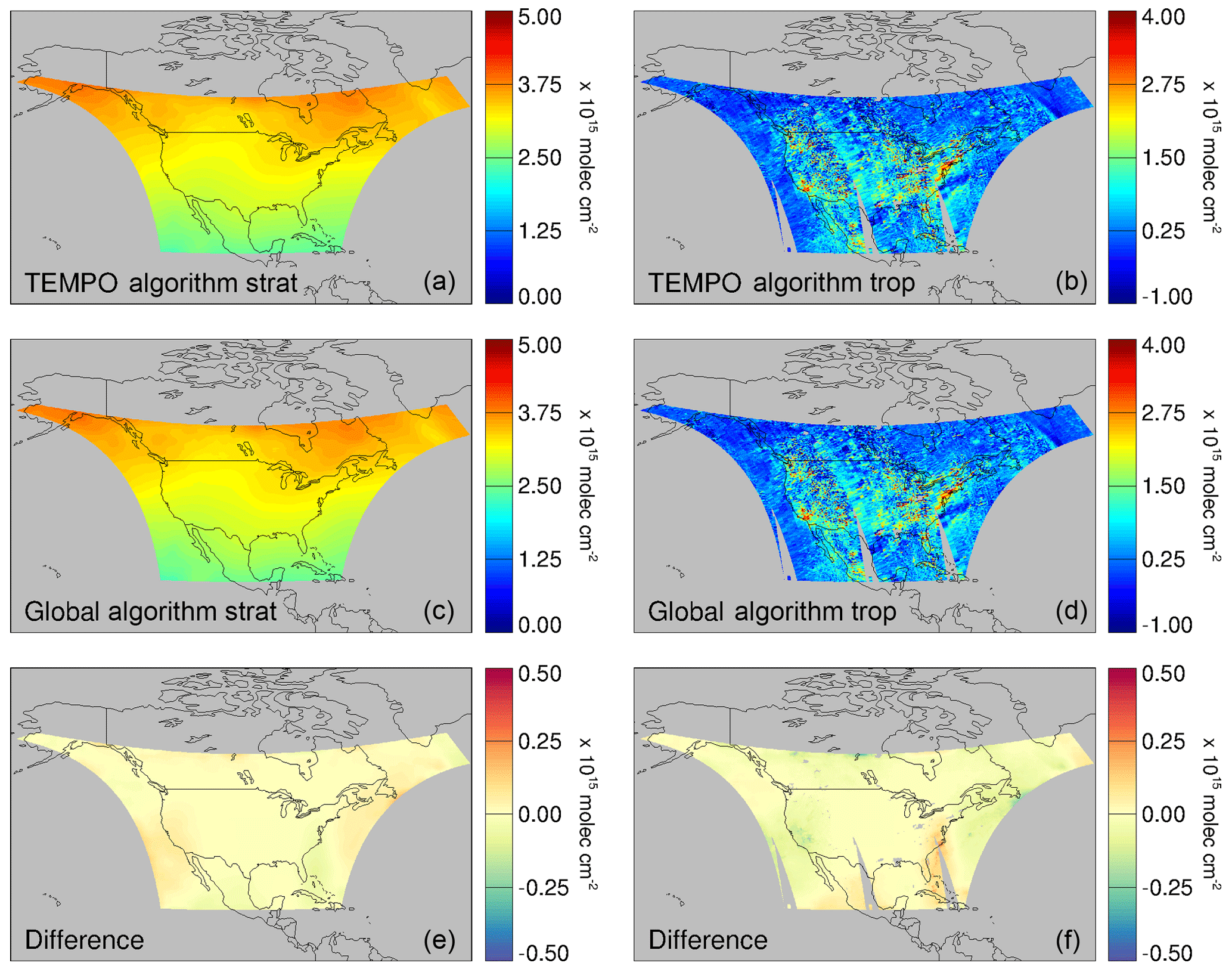
Figure 6Stratospheric NO2 (a, c, e) and final tropospheric NO2 retrievals (b, d, f) resulting from our stratosphere–troposphere separation algorithms for 15 July 2007. Panels (a, b) show the results using our proposed TEMPO algorithm. Panels (c, d) show the results using global observations (results have been clipped to the TEMPO field of regard for comparison). Panels (e, f) show the absolute differences between the TEMPO and global algorithm results.
The impact of errors in the tropospheric column due to this issue can be minimized by excluding observations with high stratospheric to tropospheric air mass factor ratios. This is also based on the logic that such values indicate tropospheric NO2 is making a small contribution to the measured signal (and as a result, the tropospheric NO2 retrieval should have high uncertainty). For this reason, we restrict all tropospheric NO2 estimates to where the local stratospheric to tropospheric air mass factor ratios are less than 5.
Figure 6 shows the stratospheric and tropospheric NO2 columns estimated for 15 July 2007. Panels (a, b) display the stratospheric and tropospheric NO2 columns as derived from our TEMPO algorithm that employs the OMI data as a surrogate for TEMPO observations, with adjacent GOME-2 data provided context outside the field of regard. Panels (c, d) display the stratospheric and tropospheric columns derived from implementing our algorithm globally with OMI data alone (the results are restricted to the TEMPO field of regard in the figure to facilitate comparison). Panels (e, f) shows the differences between our TEMPO algorithm and the global algorithm. We find excellent spatial agreement in the tropospheric NO2 estimate between the two algorithms (R2=0.997, slope=1.008). More than 95 % of the pixels have differences that are smaller than molecules cm−2.
We further evaluate the performance of our algorithm by comparing the tropospheric NO2 column distribution along the western-most edge (1∘ deep) of the TEMPO field of regard with the tropospheric NO2 tropospheric column distribution included in the independent NASA SPv3 retrieval. In this relatively remote region of the field of regard, we find a similar mean and standard deviation in column density ( molecules cm−2 in our TEMPO algorithm and molecules cm−2 in the NASA SPv3). The fraction of negative columns that are observed in our algorithm is consistent with the fraction of negative columns that occurs at the same location from the standard product (∼37 %).
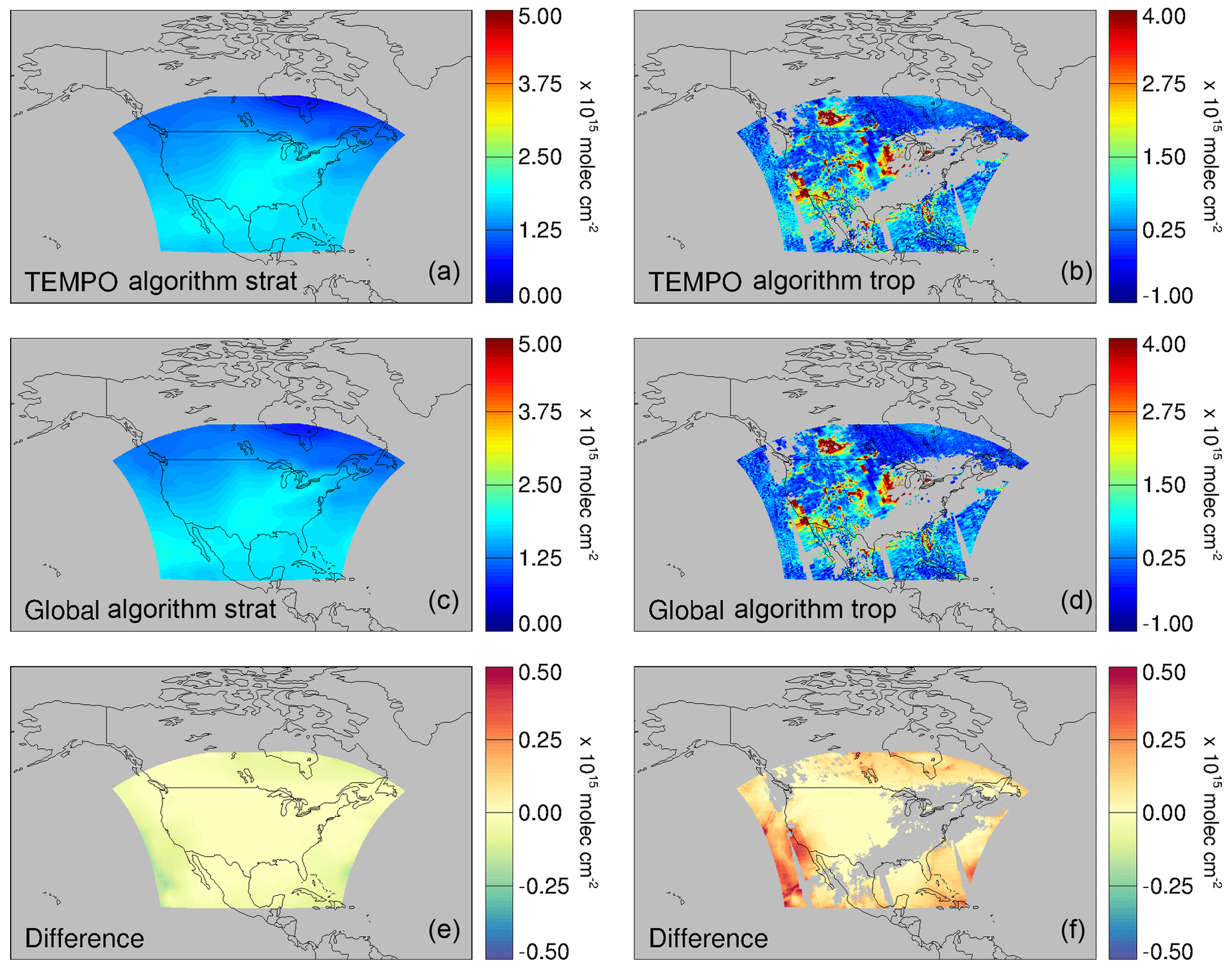
Figure 7Stratospheric NO2 (a, c, e) and final tropospheric NO2 retrievals (b, d, f) resulting from our algorithms for 15 January 2007. Panels (a, b) show the results using our proposed TEMPO algorithm. Panels (c, d) show the results using global observations (results have been clipped to the TEMPO field of regard for comparison). Panels (e, f) show the absolute differences between the TEMPO and global algorithm results.
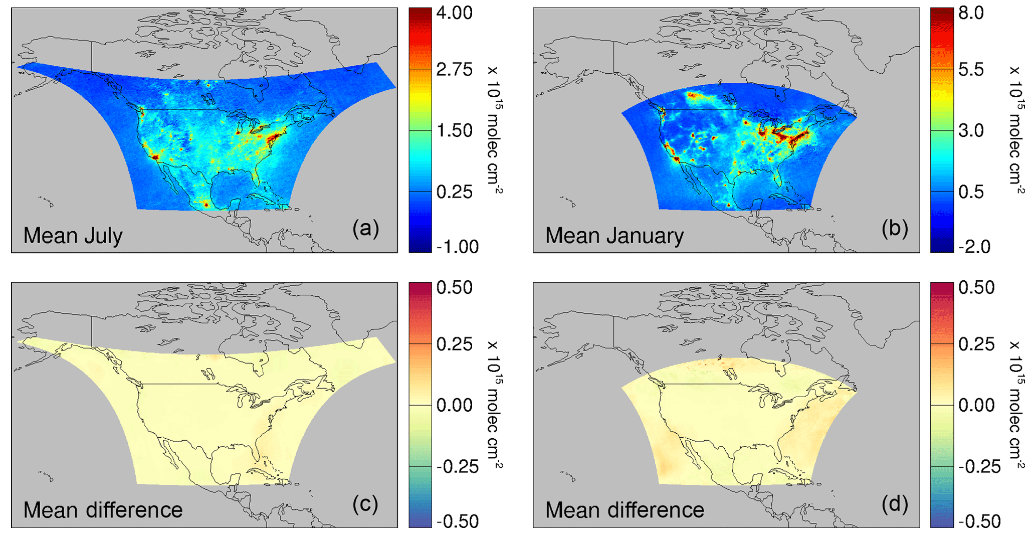
Figure 8Panels (a, b) show mean July and January tropospheric NO2 column densities resulting from our TEMPO algorithm. Panels (c, d) show absolute difference in mean July and January tropospheric NO2 between the TEMPO algorithm and the global algorithm.
Figure 7 compares the stratospheric and tropospheric NO2 column estimates from the TEMPO and global algorithms for 15 January 2007. The loss of coverage in the troposphere (mostly over the eastern US) is a result of the air mass factor issue discussed above, leading to tropospheric NO2 retrievals with low information content. The spatial agreement in the tropospheric NO2 estimates that remain is excellent across the domain (R2=0.996 slope=0.999). The magnitude of the differences in the stratospheric columns become larger in the troposphere, exceeding 0.5×10¹⁵ molecules cm−2 near the edges. Nonetheless, ∼95 % of the pixels are consistent with the global version of the algorithm to within 0.25×10¹⁵ molecules cm−2.
Figure 8 shows the monthly mean tropospheric NO2 columns resulting from our TEMPO stratosphere–troposphere separation algorithm for both July and January, and the difference vs. results from the global algorithm. We find that our TEMPO algorithm produces monthly mean results with negligible difference compared to the global algorithm, even at the field of regard edges. The correlation between the two algorithms is excellent (R2=0.999 and slope=1.009 for July, R2=0.998 and slope=0.999 for January). For July, more than 99 % of the pixels have differences that are smaller than molecules cm−2. For January, more than 90 % of the pixels have differences that are smaller than molecules cm−2, and more than 99 % of the pixels have differences that are smaller than molecules cm−2. In other words, our TEMPO-specific algorithm performs almost identically to the LEO algorithm that uses all available global data. There are some random errors near the field of regard edges on individual days (Figs. 6 and 7), but these nearly disappear in the monthly average (Fig. 8).
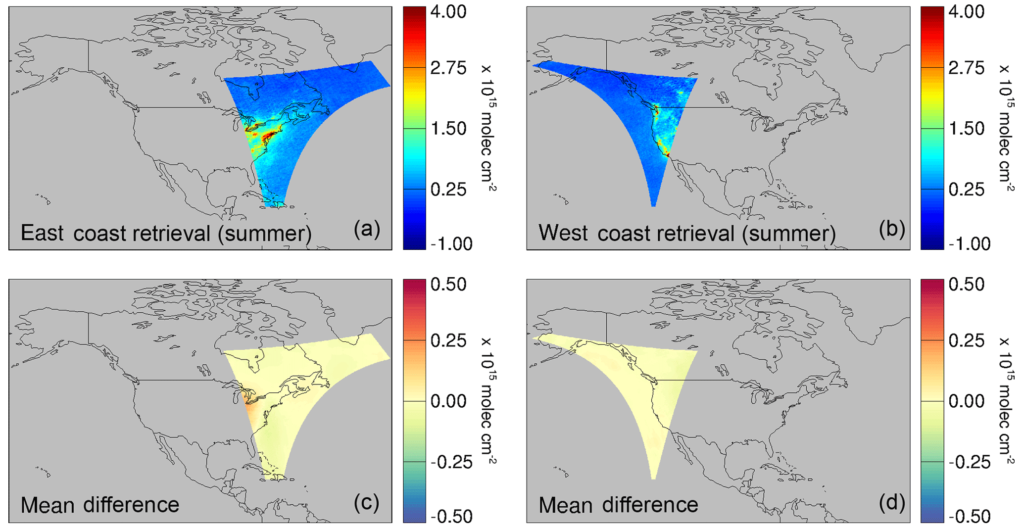
Figure 9Panels (a, b) show mean July tropospheric NO2 column densities at 11:30 UTC (a, c) and 02:00 UTC (b, d) resulting from our TEMPO STS algorithm. Panels (c, d) show absolute difference in the tropospheric NO2 column between the TEMPO algorithm and the global STS algorithm.
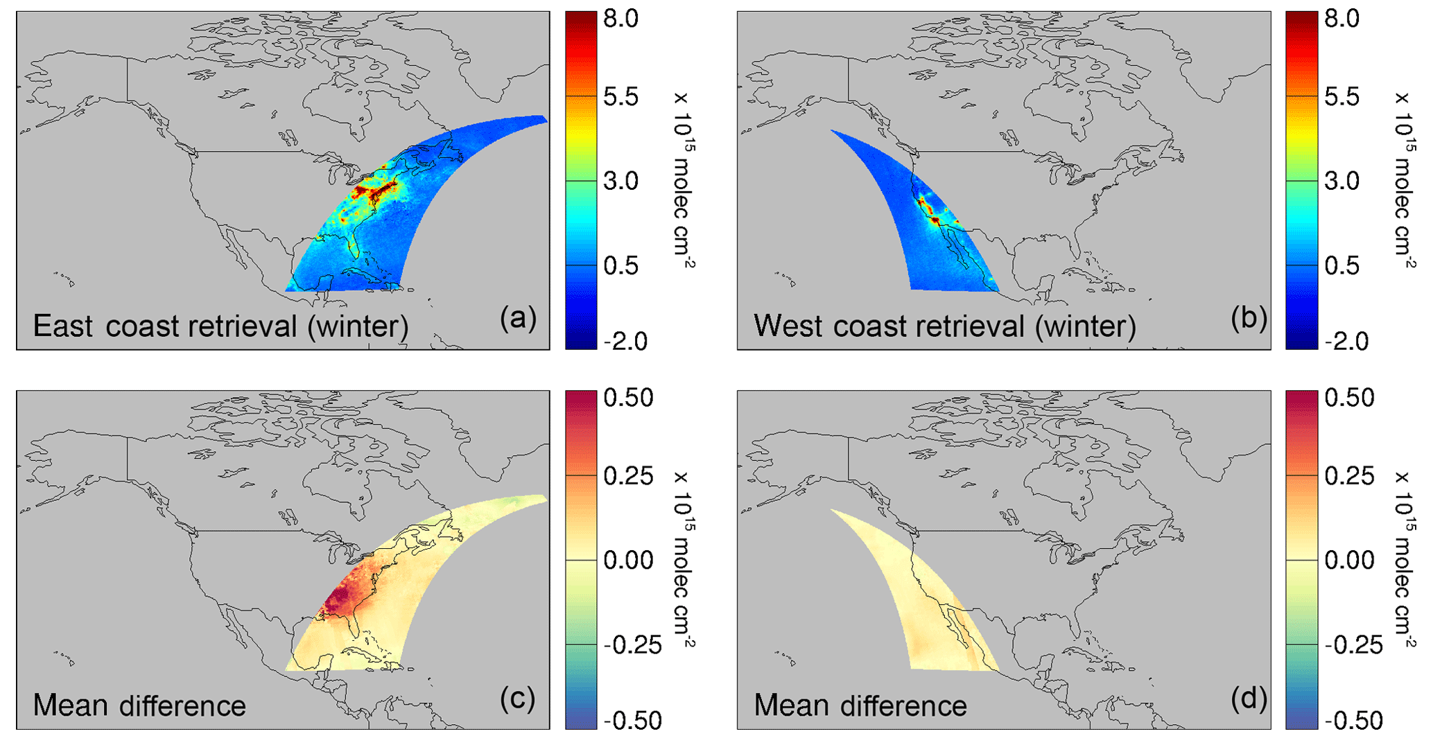
Figure 10Panels (a, b) show mean January tropospheric NO2 column densities at 14:00 UTC (a, c) and 23:30 UTC (b, d) resulting from our TEMPO STS algorithm. (c, d) show absolute difference in the tropospheric NO2 column between the TEMPO algorithm and the global STS algorithm.
Figure 9 shows the July monthly mean tropospheric NO2 columns resulting from retrievals at 11:30 UTC (east coast summer morning) and at 02:00 UTC (west coast summer evening). The east coast morning retrieval example exhibits small positive biases over some the Great Lakes region compared to the global algorithm, but overall the spatial agreement remains excellent (R2=0.996 and slope=1.015). More than 90 % of the pixels have differences that are smaller than molecules cm−2, and more than 98 % of the pixels have differences that are smaller than molecules cm−2. The west coast summer evening example also exhibits excellent performance overall (R2=0.998 and slope=0.994). In this case, more than 98 % of the pixels have differences that are smaller than molecules cm−2.
Figure 10 shows the January monthly mean tropospheric NO2 columns resulting from retrievals at 14:00 UTC (east coast winter morning) and 23:30 UTC (west coast winter evening). The bottom panels in Fig. 10 show the difference between the results from our TEMPO algorithm and the results from the global algorithm. In the east coast winter case, spatial agreement is still very good in general (R2=0.995), but we find noticeable degradation in the absolute performance over the continent compared to the global algorithm resulting from this partial field of view (slope=1.038). The west coast winter evening retrieval performs better overall (R2=0.999, slope=1.007). Although the algorithm performs poorest in the east coast winter morning case, ∼90 % of the tropospheric pixels still have differences that are less than 0.2×10¹⁵ molecules cm−2, a commonly accepted estimate of the stratospheric uncertainty resulting from stratosphere–troposphere separation in NO2 retrieval algorithms (Boersma et al., 2004). Moreover, 2 h later at 16:00 UTC when the field of regard has expanded across the Great Lakes region, into the middle of North America, and covers most of Mexico, this issue disappears (R2=0.999, slope=0.998). In other words, as spatial coverage expands, the absolute constraint on stratospheric NO2 becomes more robust.
This highlights the challenge of accurate wintertime tropospheric NO2 retrievals (especially over eastern North America) when pollution is primarily in a shallow boundary layer close to the surface where satellite remote sensing sensitivity is lowest. The partial TEMPO field of regard in this case exacerbates the problem, but the challenge is not unique to TEMPO retrievals.
Finally, we further test the performance of this algorithm at other times of day by repeating the same steps as above, but using GOME-2 observations as a surrogate for TEMPO. For this, we swap all instances of the OMI observations (overpass time ∼13:30) with GOME-2 observations (overpass time ∼09:30), and vice versa. In other words, the GOME-2 observations are restricted to the anticipated field of regard, and we use a monthly from OMI as our a priori tropospheric column and the daily observations from OMI as supporting global observations outside the TEMPO field of regard. We find the performance at this morning overpass time is as good as the mid-afternoon overpass time (R2=0.999, slope=1.005 for July; and R2=0.999, slope=1.005 for January), providing more evidence that our approach works equally well at different times of day.
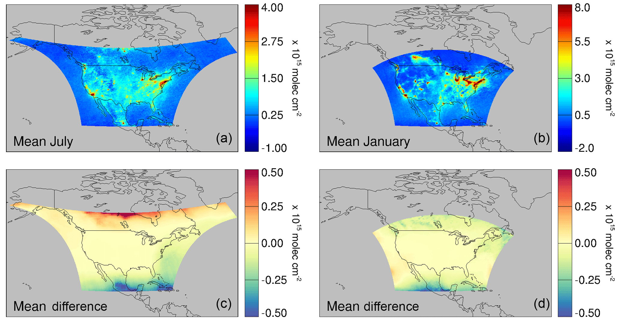
Figure 11Panels (a, b) show mean July and January tropospheric NO2 column densities resulting from our TEMPO STS algorithm without using independent low-Earth-orbit observations for context outside the TEMPO field of regard (as might be occasionally expected in near-real-time operations). Panels (c, d) show absolute difference in mean July and January tropospheric NO2 between the TEMPO algorithm and the global STS algorithm.
For retrievals in near-real time (i.e., within an hour of the observation), independent global observations in LEO may not be available (e.g., unexpected issues with LEO observation processing). Here we test the performance of the TEMPO algorithm without the supporting global observations by carrying out the identical steps outlined in Sects. 3 and 4 except without incorporating the GOME-2 observations outside the TEMPO field of regard. Comparing these results with the global algorithm isolates the penalty due to the limited TEMPO spatial domain alone, since the steps are otherwise computationally identical.
Figure 11 shows the mean July and January tropospheric columns resulting from this near-real time test. The spatial correlation with the global algorithm is still strong overall (R2=0.924 and slope=0.973 for July and R2=0.996 and slope=1.008 for January), and between 90 %–95 % of pixels in both July and January differ from the global algorithm by less than 0.2×10¹⁵ molecules cm−2. We find that, compared to a global algorithm, this stratosphere–troposphere separation approach gives rise to noticeable systematic biases near the field of regard edges (including Mexico, the Caribbean, and northern Canada). The differences are due to the lack of supporting data outside of the TEMPO field of regard.
This is most evidently a problem near the northern and southern borders of the field of regard, given the strong gradient in stratospheric NO2 as a function of latitude. At low latitudes, when the averaging windows intersect with the field of regard, the global algorithm would have lower mean values by including observations to the south. This causes the stratospheric column from the TEMPO algorithm to be systematically biased high compared to the global algorithm, translating into an underestimate in the tropospheric column (by more than molecules cm−2 in some locations). By the same logic, there is a high bias (also more than molecules cm−2 on average) along the northern edge of the field of regard in July. There are also small low biases in the tropospheric column throughout the eastern side of the TEMPO field of regard over the Atlantic Ocean. By excluding more pristine ocean conditions further to the east, the stratospheric column derived by the TEMPO algorithm is biased high compared to the global algorithm, which again translates into an underestimate in the tropospheric column.
In the absence of daily ancillary satellite data for estimating stratospheric NO2 outside the field of regard, a climatology built from satellite observations or model data could mitigate these edge effects for near real time retrievals since the average latitudinal and seasonal dependence of stratospheric NO2 are generally well known. For example, tests conducted using a monthly mean global stratospheric NO2 estimate as the supporting data outside the TEMPO field of regard improves the correlations in both cases (R2=0.999 and slope=1.010 for July and R2=0.999 and slope=1.002 for January), now with >99 % of the monthly mean pixels differing from the global algorithm results by less than 0.05×10¹⁵ molecules cm−2.

Figure 12Panels (a, b) show mean July tropospheric NO2 column densities at 11:30 UTC (a, c) and 02:00 UTC (b, d) resulting from our TEMPO STS algorithm without using independent low-Earth-orbit observations for context outside the TEMPO field of regard. Panels (c, d) show absolute difference in the tropospheric NO2 column between the TEMPO algorithm and the global STS algorithm.
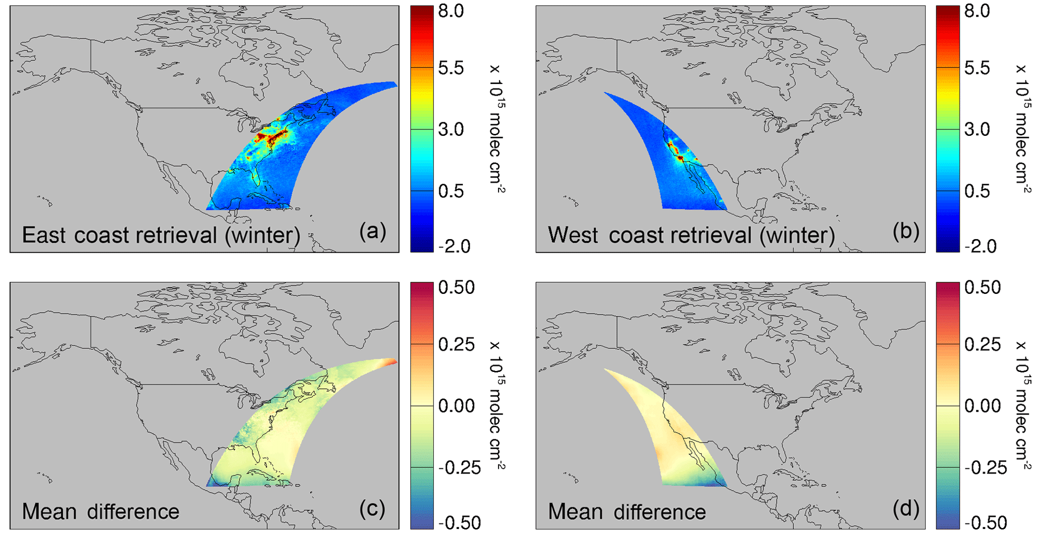
Figure 13Panels (a, b) show mean January tropospheric NO2 column densities at 14:00 UTC (a, c) and 23:30 UTC (b, d) resulting from our TEMPO STS algorithm without using independent low-Earth-orbit observations for context outside the TEMPO field of regard. (c, d) show absolute difference in the tropospheric NO2 column between the TEMPO algorithm and the global algorithm.
Similarly, we find weaker overall performance in the cases of partial fields of regard without context from surrounding LEO observations. Figure 12 shows the July mean tropospheric column retrievals calculated for 11:30 UTC (east coast summer morning) and the July mean tropospheric column retrievals for 02:00 UTC (west coast summer evening). Though this version of the algorithm performs less well compared to the results from incorporating independent LEO observations, the spatial correlation is still good (R2=0.944, slope=0.943 for 11:30 UTC July; R2=0.964, slope=0.986 for 02:00 UTC). The differences over most of the available domain remain small, with 90 %–95 % of the pixels having differences in the mean tropospheric column of less than molecules cm−2 compared to the global algorithm. Figure 13 shows the January mean tropospheric column retrievals calculated for 14:00 UTC (east coast winter morning) and the January mean tropospheric column retrievals for 23:00 UTC (west coast winter evening). The spatial correlation in both cases remains strong, again with some systematic biases observed (R2=0.996, slope=1.001 at 14:00 UTC and R2=0.987, slope=1.019 at 23:30 UTC). The biases remain modest, with ∼90 % of the pixels being consistent to within 0.2×1015 cm−2 of the global implementation of the algorithm. Again, using a monthly climatology mitigates the biases in all cases, with the smallest improvement for the retrieval in January at 14:00 UTC (going from 90 % to 94 % of the pixels being consistent to within 0.2×1015 cm−2 of the global implementation of the algorithm).
Given these results, our recommendation for TEMPO is to use a climatological estimate (e.g., a 30-day mean) of stratospheric NO2 for context outside of the TEMPO field of regard during near-real-time retrieval if LEO observations are unavailable. This climatological estimate can be constructed based on satellite-derived observations in LEO from the preceding year and corrected for the time of day based on model results or other independent observations. We would then propose a subsequent reprocessing of the data that incorporates the daily LEO observations when available from the correct observation day.
The TEMPO geostationary satellite instrument is expected to provide hourly observations of NO2 columns (among a variety of other measurements) over North America. Here, we have developed and tested the first stratosphere–troposphere separation algorithm for TEMPO geostationary satellite observations of atmospheric NO2 column density. We use independent measurements from a low-Earth-observing satellite instrument to identify likely locations of tropospheric enhancements, and to provide context outside of the available TEMPO measurements. We consider partial fields of regard as a function of time of day, and implement a new filter based on stratospheric to tropospheric air mass factor ratios. We investigate in particular the information penalty associated with the limited TEMPO fields of regard as a function of season and time of day.
We find that our algorithm performs as well as a global LEO algorithm for most scenarios. When the whole continent is observed, monthly mean agreement with tropospheric NO2 retrieved from the global algorithm is excellent (R2=0.999, slope=1.009 for July and R2=0.998, slope=0.999 January). During most instances with a partial field of regard (e.g., east coast morning or west coast evening) the algorithm still performs robustly. We demonstrate that small biases near the southern and northern edges of the field of regard are avoided by incorporating independent LEO observations that have been corrected for the time of day. When the whole continent is observed, the vast majority of pixels (>95 %) agree with results from a global implementation of the same algorithm to within molecules cm−2. We find that the TEMPO algorithm is challenged most by winter east coast morning retrievals, but nonetheless the difference between the TEMPO algorithm and the global implementation of the same algorithm produces differences that are less than 0.2×10¹⁵ molecules cm−2 for more than 90 % of the pixels. Even when supporting observations from LEO may not be available (as in near-real-time), a large majority of pixels (∼90 % or greater) agree with the global algorithm to within molecules cm−2 on a monthly mean basis, which is generally accepted as typical estimates of stratospheric error due to stratosphere–troposphere separation algorithms. The differences can be reduced further in near-real-time retrievals by the use of a climatology outside the TEMPO field of regard. The value of independent LEO observations for TEMPO tropospheric retrievals implies benefit to TEMPO data from ongoing development of LEO observations.
We have demonstrated a feasible and robust stratosphere–troposphere separation algorithm for the retrieval of geostationary satellite-based NO2 tropospheric column densities by the TEMPO instrument notwithstanding the limited field of regard or changing time of day. Our TEMPO algorithm also demonstrates good performance when evaluated against the stratospheric NO2 columns provided with the NASA SPv3 standard product, but further independent evaluation using ground-based spectrometer network observations will be beneficial. This approach may be applicable to other planned geostationary satellite instruments including Sentinel-4 over Europe and GEMS over Asia. This spatial filtering and interpolation method may also have applications in offset removal during retrievals of HCHO and SO2 tropospheric columns.
Data from this study, and the algorithm developed for TEMPO, are available upon request by contacting the first author: jgeddes@bu.edu.
The authors declare that they have no conflict of interest.
The authors are grateful to Kelly Chance, Xiong Liu, John Houck, Peter Zoogman,
and other members of the TEMPO trace gas retrieval team for their input
in preparation of this paper. Work at Dalhousie University was
supported by Environment and Climate Change Canada. The authors also
gratefully acknowledge the free use of TEMIS NO2 data from the GOME-2
sensor provided by http://www.temis.nl, last access: 12 November 2018, and the NASA Standard Product
NO2 data from OMI provided by https://disc.gsfc.nasa.gov/datasets/OMNO2_V003/summary, last access: 9 November 2018.
Edited by: Folkert Boersma
Reviewed by: two anonymous referees
Adams, C., Normand, E. N., McLinden, C. A., Bourassa, A. E., Lloyd, N. D., Degenstein, D. A., Krotkov, N. A., Belmonte Rivas, M., Boersma, K. F., and Eskes, H.: Limb–nadir matching using non-coincident NO2 observations: proof of concept and the OMI-minus-OSIRIS prototype product, Atmos. Meas. Tech., 9, 4103–4122, https://doi.org/10.5194/amt-9-4103-2016, 2016.
Bechle, M. J., Millet, D. B., and Marshall, J. D.: Remote sensing of exposure to NO2: Satellite versus ground-based measurement in a large urban area, Atmos. Environ., 69, 345–353, https://doi.org/10.1016/j.atmosenv.2012.11.046, 2013.
Beirle, S., Platt, U., Wenig, M., and Wagner, T.: Weekly cycle of NO2 by GOME measurements: a signature of anthropogenic sources, Atmos. Chem. Phys., 3, 2225–2232, https://doi.org/10.5194/acp-3-2225-2003, 2003.
Beirle, S., Kühl, S., Puķīte, J., and Wagner, T.: Retrieval of tropospheric column densities of NO2 from combined SCIAMACHY nadir/limb measurements, Atmos. Meas. Tech., 3, 283–299, https://doi.org/10.5194/amt-3-283-2010, 2010.
Beirle, S., Hörmann, C., Jöckel, P., Liu, S., Penning de Vries, M., Pozzer, A., Sihler, H., Valks, P., and Wagner, T.: The STRatospheric Estimation Algorithm from Mainz (STREAM): estimating stratospheric NO2 from nadir-viewing satellites by weighted convolution, Atmos. Meas. Tech., 9, 2753–2779, https://doi.org/10.5194/amt-9-2753-2016, 2016.
Boersma, K. F., Eskes, H. J., and Brinksma, E. J.: Error analysis for tropospheric NO2 retrieval from space, J. Geophys. Res., 109, D04311–D04311, https://doi.org/10.1029/2003JD003962, 2004.
Boersma, K. F., Eskes, H. J., Veefkind, J. P., Brinksma, E. J., van der A, R. J., Sneep, M., van den Oord, G. H. J., Levelt, P. F., Stammes, P., Gleason, J. F., and Bucsela, E. J.: Near-real time retrieval of tropospheric NO2 from OMI, Atmos. Chem. Phys., 7, 2103–2118, https://doi.org/10.5194/acp-7-2103-2007, 2007.
Boersma, K. F., Jacob, D. J., Eskes, H. J., Pinder, R. W., Wang, J., and van der A, R. J.: Intercompariso of SCIAMACHY and OMI tropospheric NO2 columns: Observing the diural evolutio of chemistry and emissios from space, J. Geophys. Res., 113(D16), D16S26, https://doi.org/10.1029/2007JD008816, 2008.
Boersma, K. F., Jacob, D. J., Trainic, M., Rudich, Y., DeSmedt, I., Dirksen, R., and Eskes, H. J.: Validation of urban NO2 concentrations and their diurnal and seasonal variations observed from the SCIAMACHY and OMI sensors using in situ surface measurements in Israeli cities, Atmos. Chem. Phys., 9, 3867–3879, https://doi.org/10.5194/acp-9-3867-2009, 2009.
Bovensmann, H., Burrows, J. P., Buchwitz, M., Frerick, J., Noël, S., Rozanov, V. V., Chance, K. V., Goede, A. P. H., Bovensmann, H., Burrows, J. P., Buchwitz, M., Frerick, J., Noël, S., Rozanov, V. V., Chance, K. V., and Goede, A. P. H.: SCIAMACHY: Mission Objectives and Measurement Modes, J. Atmos. Sci., 56, 127–150, https://doi.org/10.1175/1520-0469(1999)056<0127:SMOAMM>2.0.CO;2, 1999.
Bucsela, E. J., Celarier, E. A., Wenig, M. O., Gleason, J. F., Veefkind, J. P., Boersma, K. F., and Brinksma, E. J.: Algorithm for NO2 vertical column retrieval from the ozone monitoring instrument, IEEE T. Geosci. Remote, 44, 1245–1257, 2006.
Bucsela, E. J., Krotkov, N. A., Celarier, E. A., Lamsal, L. N., Swartz, W. H., Bhartia, P. K., Boersma, K. F., Veefkind, J. P., Gleason, J. F., and Pickering, K. E.: A new stratospheric and tropospheric NO2 retrieval algorithm for nadir-viewing satellite instruments: applications to OMI, Atmos. Meas. Tech., 6, 2607–2626, https://doi.org/10.5194/amt-6-2607-2013, 2013.
Courrege-Lacoste, G. B., Sallusti, M., Bulsa, G., Bagnasco, G., Veihelmann, B., Riedl, S., Smith, D. J., and Maurer, R.: The Copernicus Sentinel 4 mission – A Geostationary Imaging UVN Spectrometer for Air Quality Monitoring, in: Proceedings of SPIE Sensors, Systems, and Next-Generation Satellites XXI, 10423, 1042307, https://doi.org/10.1117/12.2282158, 2017.
Dirksen, R. J., Boersma, K. F., Eskes, H. J., Ionov, D. V., Bucsela, E. J., Levelt, P. F., and Kelder, H. M.: Evaluation of stratospheric NO2 retrieved from the Ozone Monitoring Instrument: Intercomparison, diurnal cycle, and trending, J. Geophys. Res., 116, D08305, https://doi.org/10.1029/2010JD014943, 2011.
Duncan, B. N., Yoshida, Y., de Foy, B., Lamsal, L. N., Streets, D. G., Lu, Z., Pickering, K. E., and Krotkov, N. A.: The observed response of Ozone Monitoring Instrument (OMI) NO2 columns to NOx emission controls on power plants in the United States: 2005–2011, Atmos. Environ., 81, 102–111, https://doi.org/10.1016/j.atmosenv.2013.08.068, 2013.
Finlayson-Pitts, B. and Pitts, J.: Chemistry of the Upper and Lower Atmosphere. Theory, Experiments, and Applications, Academic Press, New York, 1999.
Geddes, J. A. and Martin, R. V.: Global deposition of total reactive nitrogen oxides from 1996 to 2014 constrained with satellite observations of NO2 columns, Atmos. Chem. Phys., 17, 10071–10091, https://doi.org/10.5194/acp-17-10071-2017, 2017.
Geddes, J. A., Martin, R. V., Boys, B. L., and van Donkelaar, A.: Long-Term Trends Worldwide in Ambient NO2 Concentrations Inferred from Satellite Observations, Environ. Health Perspect., 124, 281–289, https://doi.org/10.1289/ehp.1409567, 2016.
Hilboll, A., Richter, A., Rozanov, A., Hodnebrog, Ø., Heckel, A., Solberg, S., Stordal, F., and Burrows, J. P.: Improvements to the retrieval of tropospheric NO2 from satellite – stratospheric correction using SCIAMACHY limb/nadir matching and comparison to Oslo CTM2 simulations, Atmos. Meas. Tech., 6, 565–584, https://doi.org/10.5194/amt-6-565-2013, 2013.
Ialongo, I., Herman, J., Krotkov, N., Lamsal, L., Boersma, K. F., Hovila, J., and Tamminen, J.: Comparison of OMI NO2 observations and their seasonal and weekly cycles with ground-based measurements in Helsinki, Atmos. Meas. Tech., 9, 5203–5212, https://doi.org/10.5194/amt-9-5203-2016, 2016.
Jaegle, L., Steinberger, L., Martin, R. V., and Chance, K.: Global partitioning of NOx sources using satellite observations: Relative roles of fossil fuel combustion, biomass burning and soil emissions, Faraday Discuss., 130, 407–423, https://doi.org/10.1039/b502128f, 2005.
Jia, Y., Yu, G., Gao, Y., He, N., Wang, Q., Jiao, C., and Zuo, Y.: Global inorganic nitrogen dry deposition inferred from ground- and space-based measurements., Sci. Rep.-UK, 6, 19810, https://doi.org/10.1038/srep19810, 2016.
Konovalov, I. B., Beekmann, M., Burrows, J. P., and Richter, A.: Satellite measurement based estimates of decadal changes in European nitrogen oxides emissions, Atmos. Chem. Phys., 8, 2623–2641, https://doi.org/10.5194/acp-8-2623-2008, 2008.
Krotkov, N. A., Lamsal, L. N., Celarier, E. A., Swartz, W. H., Marchenko, S. V., Bucsela, E. J., Chan, K. L., Wenig, M., and Zara, M.: The version 3 OMI NO2 standard product, Atmos. Meas. Tech., 10, 3133–3149, https://doi.org/10.5194/amt-10-3133-2017, 2017.
Lamsal, L. N., Martin, R. V., van Donkelaar, A., Steinbacher, M., Celarier, E. A., Bucsela, E., Dunlea, E. J., and Pinto, J. P.: Ground-level nitrogen dioxide concenrations inferred from the satellite-borne Ozone Monitoring Instrument, J. Geophys. Res.-Atmos., 113, D16308, https://doi.org/10.1029/2007JD009235, 2008.
Lamsal, L. N., Martin, R. V, Padmanabhan, A., Van Donkelaar, A., Zhang, Q., Sioris, C. E., Chance, K., Kurosu, T. P., and Newchurch, M. J.: Application of satellite observations for timely updates to global anthropogenic NOx emission inventories, Geophys. Res. Lett., 38, L05810, https://doi.org/10.1029/2010GL046476, 2011.
Lamsal, L. N., Krotkov, N. A., Celarier, E. A., Swartz, W. H., Pickering, K. E., Bucsela, E. J., Gleason, J. F., Martin, R. V., Philip, S., Irie, H., Cede, A., Herman, J., Weinheimer, A., Szykman, J. J., and Knepp, T. N.: Evaluation of OMI operational standard NO2 column retrievals using in situ and surface-based NO2 observations, Atmos. Chem. Phys., 14, 11587–11609, https://doi.org/10.5194/acp-14-11587-2014, 2014.
Lasnik, J., Stephens, M., Baker, B., Randall, C., Ko, D. H., Kim, S., Kim, Y., Lee, E. S., Chang, S., Park, J.-M., Seo, S.-B., Youk, Y., Kong, J. P., Lee, D., Lee, S.-H., and Kim, J.: Geostationary Environment Monitoring Spectrometer (GEMS) over the Korea peninsula and Asia-Pacific region. Abstract A51A-3003 presented at 2014 Fall Meeting, AGU, 15–19 December 2014, San Francisco, California, 2014.
Leue, C., Wenig, M., Wagner, T., Klimm, O., Platt, U., and Jähne, B.: Quantitative analysis of NOx emissions from Global Ozone Monitoring Experiment satellite image sequences, J. Geophys. Res.-Atmos., 106, 5493–5505, https://doi.org/10.1029/2000JD900572, 2001.
Martin, R. V., Chance, K., Jacob, D. J., Kurosu, T. P., Spurr, R. J. D., Bucsela, E., Gleason, J. F., Palmer, P. I., Bey, I., Fiore, A. M., Li, Q., Yantosca, R. M., and Koelemeijer, R. B. A.: An improved retrieval of tropospheric nitrogen dioxide from GOME, J. Geophys. Res., 107, 4437, https://doi.org/10.1029/2001JD001027, 2002.
Martin, R. V., Jacob, D. J., Chance, K., Kurosu, T. P., Palmer, P. I., and Evans, M. J.: Global inventory of nitrogen oxide emissions constrained by space-based observations of NO2 columns, J. Geophys. Res., 108, 4537, https://doi.org/10.1029/2003JD003453, 2003.
McLinden, C. A., Fioletov, V., Boersma, K. F., Krotkov, N., Sioris, C. E., Veefkind, J. P., and Yang, K.: Air quality over the Canadian oil sands: A first assessment using satellite observations, Geophys. Res. Lett., 39, L04804, https://doi.org/10.1029/2011GL050273, 2012.
Miyazaki, K., Eskes, H., Sudo, K., Boersma, K. F., Bowman, K., and Kanaya, Y.: Decadal changes in global surface NOx emissions from multi-constituent satellite data assimilation, Atmos. Chem. Phys., 17, 807–837, https://doi.org/10.5194/acp-17-807-2017, 2017.
Nowlan, C. R., Martin, R. V., Philip, S., Lamsal, L. N., Krotkov, N. A., Marais, E. A., Wang, S., and Zhang, Q.: Global dry deposition of nitrogen dioxide and sulfur dioxide inferred from space-based measurements, Global Biogeochem. Cycles, 28, 1025–1043, https://doi.org/10.1002/2014GB004805, 2014.
Richter, A. and Burrows, J. P.: Tropospheric NO2 from GOME measurements, Adv. Space Res., 29, 1673–1683, https://doi.org/10.1016/S0273-1177(02)00100-X, 2002.
Richter, A., Burrows, J. P., Nüss, H., Granier, C., and Niemeier, U.: Increase in tropospheric nitrogen dioxide over China observed from space, Nature, 437, 1025–1043, https://doi.org/10.1038/nature04092, 2005.
Russell, A. R., Valin, L. C., and Cohen, R. C.: Trends in OMI NO2 observations over the United States: effects of emission control technology and the economic recession, Atmos. Chem. Phys., 12, 12197–12209, https://doi.org/10.5194/acp-12-12197-2012, 2012.
Seinfeld, J. H. and Pandis, S. N.: Atmospheric Chemistry and Physics: from air pollution to climate change, 3rd ed., John Wiley & Sons Inc., Hoboken, New Jersey, 2016.
Sussmann, R., Stremme, W., Burrows, J. P., Richter, A., Seiler, W., and Rettinger, M.: Stratospheric and tropospheric NO2 variability on the diurnal and annual scale: a combined retrieval from ENVISAT/SCIAMACHY and solar FTIR at the Permanent Ground-Truthing Facility Zugspitze/Garmisch, Atmos. Chem. Phys., 5, 2657–2677, https://doi.org/10.5194/acp-5-2657-2005, 2005.
Valks, P., Pinardi, G., Richter, A., Lambert, J.-C., Hao, N., Loyola, D., Van Roozendael, M., and Emmadi, S.: Operational total and tropospheric NO2 column retrieval for GOME-2, Atmos. Meas. Tech., 4, 1491–1514, https://doi.org/10.5194/amt-4-1491-2011, 2011.
Velders, G. J. M., Granier, C., Portmann, R. W., Pfeilsticker, K., Wenig, M., Wagner, T., Platt, U., Richter, A., and Burrows, J. P.: Global tropospheric NO2 column distributions: Comparing three-dimensional model calculations with GOME measurements, J. Geophys. Res.-Atmos., 106, 12643–12660, https://doi.org/10.1029/2000JD900762, 2001.
Wenig, M., Kühl, S., Beirle, S., Bucsela, E., Jähne, B., Platt, U., Gleason, J., and Wagner, T.: Retrieval and analysis of stratospheric NO2 from the Global Ozone Monitoring Experiment, J. Geophys. Res.-Atmos., 109, D04315, https://doi.org/10.1029/2003JD003652, 2004.
Zoogman, P., Liu, X., Suleiman, R. M., Pennington, W. F., Flittner, D. E., Al-Saadi, J. A., Hilton, B. B., Nicks, D. K., Newchurch, M. J., Carr, J. L., Janz, S. J., Andraschko, M. R., Arola, A., Baker, B. D., Canova, B. P., Chan Miller, C., Cohen, R. C., Davis, J. E., Dussault, M. E., Edwards, D. P., Fishman, J., Ghulam, A., González Abad, G., Grutter, M., Herman, J. R., Houck, J., Jacob, D. J., Joiner, J., Kerridge, B. J., Kim, J., Krotkov, N. A., Lamsal, L., Li, C., Lindfors, A., Martin, R. V., McElroy, C. T., McLinden, C., Natraj, V., Neil, D. O., Nowlan, C. R., O'Sullivan, E. J., Palmer, P. I., Pierce, R. B., Pippin, M. R., Saiz-Lopez, A., Spurr, R. J. D., Szykman, J. J., Torres, O., Veefkind, J. P., Veihelmann, B., Wang, H., Wang, J., and Chance, K.: Tropospheric emissions: Monitoring of pollution (TEMPO), J. Quant. Spectrosc. Ra., 186, 17–39, https://doi.org/10.1016/j.jqsrt.2016.05.008, 2017.