the Creative Commons Attribution 4.0 License.
the Creative Commons Attribution 4.0 License.
 | 21 Nov 2018
The impact of MISR-derived injection height initialization on wildfire and volcanic plume dispersion in the HYSPLIT model
Charles J. Vernon
Ryan Bolt
Timothy Canty
Ralph A. Kahn
The dispersion of particles from wildfires, volcanic eruptions, dust storms, and other aerosol sources can affect many environmental factors downwind, including air quality. Aerosol injection height is one source attribute that mediates downwind dispersion, as wind speed and direction can vary dramatically with elevation. Using plume heights derived from space-based, multi-angle imaging, we examine the impact of initializing plumes in the NOAA Air Resources Laboratory's Hybrid Single-Particle Lagrangian Integrated Trajectory (HYSPLIT) model with satellite-measured vs. nominal (model-calculated or VAAC-reported) injection height on the simulated dispersion of six large aerosol plumes. When there are significant differences in nominal vs. satellite-derived particle injection heights, especially if both heights are in the free troposphere or if one injection height is within the planetary boundary layer (PBL) and the other is above the PBL, differences in simulation results can arise. In the cases studied with significant nominal vs. satellite-derived injection height differences, the HYSPLIT model can represent plume evolution better, relative to independent satellite observations, if the injection height in the model is constrained by hyper-stereo satellite retrievals.
- Article
(16009 KB) -
Supplement
(66137 KB) - BibTeX
- EndNote


More than 5.5 million people worldwide die prematurely every year due to household and outdoor air pollution (Forouzanfar et al., 2015). Model forecasting of airborne particle dispersion is the essential tool used to alert citizens to possible poor air quality conditions, as well as to assess longer term exposure. Aerosol plume height is a key input to these models (Walter et al., 2016). The height of aerosol plumes produced by wildfires, volcanic eruptions, and dust storms has a large influence on where the particles are transported, and their environmental impacts. If aerosols are injected into the atmosphere above the planetary boundary layer (PBL) – or if they are entrained into the free troposphere after injection – they can be transported vast distances by free-tropospheric winds, causing aviation hazards, impacting regional-scale temperatures, cloud properties, and precipitation, and ultimately affecting ground-level air quality at great distances from the source (e.g., Colarco et al., 2004). In this study, we use hyper-stereo imagery from the NASA Earth Observing System's multi-angle imaging spectroradiometer (MISR) instrument to map aerosol plume heights. The stereo technique provides plume heights with reasonable certainty in near-source regions, where features in the plume can be identified in multiple, angular views (e.g., Nelson et al., 2013). Depending on plume properties, stereo plume-height retrieval can extend to tens or even hundreds of kilometers downwind from the source.
1.1 Multi-angle imaging spectroradiometer (MISR) and moderate resolution imaging spectroradiometer (MODIS)
The MISR instrument flies aboard the Terra satellite, in the AM constellation of the NASA Earth Observing System (EOS). Terra is in a near-polar orbit at an altitude of 705 km, descending on the dayside, with equator crossing at Local Time, and completes an orbit in about 99 min. Each circuit of the Earth falls into one of 233 overlapping “paths” that repeat precisely every 16 days (Diner et al., 1998). The instrument acquires imagery at nine angles ranging from 0 (nadir) to 70.5∘ off-nadir in the forward and aft directions along-track, in each of four spectral bands centered at 446 (blue), 558 (green), 672 (red), and 866 nm (near infrared, NIR). The 70.5∘ viewing cameras are sometimes designated “Df” and “Da” for fore- and aft-viewing, respectively. The “C” and “B” cameras view at 60.0 and 45.6∘, respectively, and the three “A” cameras view at 26.1∘ or nadir. Data are acquired routinely at 275 m horizontal resolution in the nadir view and in the red band of the other eight cameras; all other channels are obtained at 1.1 km resolution. The MISR design allows it to image within 7 min for every scene at nine viewing zenith angles along the satellite ground track. The width of the MISR swath common to all cameras is about 380 km, providing global coverage every 9 days at the equator and every 2 days near the poles. The MISR plume-height products are derived from the hyper-stereo imagery geometrically, and take account of the proper motion of plume elements (Muller et al., 2002; Nelson et al., 2013). This retrieval approach requires contrast features in the plume to be visible in the multi-angle data. As such, MISR plume-height mapping complements aerosol height curtains obtained from space-based lidar; lidar offers sensitivity to thin aerosol layers downwind of sources, where plume features required for stereo image matching are lacking, but the active sensor offers vastly less spatial coverage, so the actual source regions are seldom observed (Kahn et al., 2008).
We also use context imagery from the two moderate resolution imaging spectroradiometer (MODIS) instruments; one flies aboard the Terra satellite with MISR, providing coincident observations, and the other is aboard NASA's Aqua satellite, which crosses the Equator at Local Time on the day side. MODIS is a wide-swath, multi-spectral, single-view imager that acquires data over the entire planet every day or two, depending on latitude. MODIS can track the development of aerosol plumes over several days, allowing us to compare plume evolution, as simulated by different model runs, with imagery and aerosol optical depth (AOD) retrievals from MODIS.
1.2 The MISR interactive explorer (MINX)
To apply the multi-angle capabilities of MISR most effectively for mapping aerosol plume height, the MISR interactive explorer (MINX) visualization application was developed (Nelson et al., 2008, 2013), complementing the fully automatic but less accurate operational MISR stereo product (Moroney et al., 2002; Muller et al., 2002). MINX offers users a tool to retrieve height and wind information interactively at high spatial resolution and enhanced precision. Users operating the MINX interface must manually identify the horizontal extent of the plume in the imagery, the source point, and the wind direction; as full coverage of a scene by the nine MISR cameras takes 7 min, there is enough time to observe the motion of the plume. By viewing an animation of these images in sequence, a user can determine wind direction. This quantity can also be calculated directly by fitting the parallax and the apparent motion of the scene self-consistently, but, in practice, user determination of wind direction reduces uncertainty. Some user discretion is involved, especially if significant wind runs along-track, as small differences in the choice of wind direction can affect the resulting wind speed, the associated wind correction, and the height retrieval (Nelson et al., 2013). Vertical resolution is between about 275 and 500 m, depending on observing conditions. This makes it possible to study the 3-D context of a scene, and allows the user to detect scene content that would otherwise be difficult to discern in single-view imagery from more conventional satellite instruments such as MODIS. In practice, red and blue bands are used separately to determine both zero-wind and wind-corrected plume height. The choice of one band over another depends upon the differences in spatial resolution and contrast with the surface in each case. The blue band has poorer horizontal resolution (1.1 km), which results in poorer vertical resolution (∼500 m) due to the geometric nature of the retrieval. However, aerosol plumes tend to be optically thicker at the blue than red wavelengths, so the blue band offers enhanced contrast with the surface. This can be important for optically thin plume retrievals. The red band provides higher horizontal (and therefore also vertical) resolution (∼275 m). In the current study, red-band MINX retrievals were generally favored, because the plumes selected are all optically thick enough to be observed well in this band. For further details, see Nelson et al. (2013).
1.3 The HYSPLIT model
The National Oceanic and Atmospheric Administration (NOAA) Air Resources Laboratory's (ARL) Hybrid Single-Particle Lagrangian Integrated Trajectory model (HYSPLIT) is a complete system for computing simple air parcel trajectories as well as complex transport, dispersion, chemical transformation, and deposition simulations. HYSPLIT continues to be one of the most extensively used atmospheric transport and dispersion models in the atmospheric sciences community (Stein et al., 2015). In other studies, HYSPLIT has been used to track and forecast the release of radioactive material, wildfire smoke, wind-blown dust, pollutants from various stationary and mobile emission sources, allergens, and volcanic ash (e.g., Stunder et al., 2007; Kahn and Limbacher, 2012; Crawford et al., 2016). The model calculation method can be Lagrangian, using a moving frame of reference for advection and diffusion calculations as the air parcels move from their initial location, Eulerian, which uses a fixed three-dimensional grid as a frame of reference to compute pollutant air concentrations, or a hybrid combination of the two approaches (Stein et al., 2015).
As with any such model, several factors can limit the accuracy of simulations, including uncertainty in the simulated wind structure, the location and strength of aerosol sources, and, most relevant for the current study, input pollutant injection height (Stein et al., 2009). Since the late 1990s, “the IAVW (International Airways Volcano Watch) has recognized that more accurate source parameters are needed to improve model accuracy, especially in the first hours of an eruption when few observations may be available” (Mastin et al., 2009). Although MISR data are acquired over a given location on Earth only about once per week on average, when available, we expect these observations to improve forecasted plume dispersion, at least in some cases. In this paper we explore the impact of using the unique data provided from MISR–MINX to obtain direct-source initial conditions as input to HYSPLIT. Using more accurate plume heights, we run the HYSPLIT dispersion model and compare the results with those obtained using the model's nominal injection height and with the actual dispersion of the plume as observed by MODIS.
We chose specific wildfire and volcanic eruption cases where the MINX retrievals are available and of high quality. MINX retrievals are not available for specific events if MISR does not have coverage or if there is significant cloud contamination of the scene. The quality of a case is determined by two factors: (1) a lack of cloud contamination and (2) sufficient aerosol optical thickness so plume contrast features are clearly visible in the imagery and distinct from the surface. The optical thickness criterion is assessed through visual inspection of each scene using the MINX camera animation function. The six cases selected for this study are (1) the Mount Etna eruption of July 2001, (2) the Chikurachki Volcano eruption of April 2003, (3) the Eyjafjallajökull eruption of May 2010, (4) the Fort McMurray fires of May 2016, (5) the Fraser Plateau fires of August 2017, and (6) the Thomas fires of December 2017.
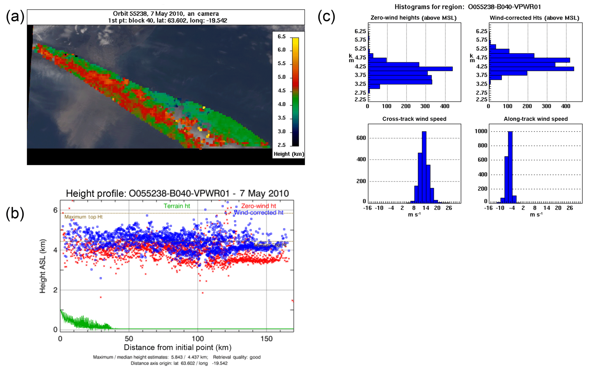
Figure 1MINX height retrievals, measured from the geoid, for the Eyjafjallajökull volcano eruption plume, 7 May 2010. (a) Elevation map for the main plume. Each box represents a 0.55 km area where the height is displayed with darker colors on the low end and warmer colors on the high end. (b) MINX height profile, as a function of distance from the source. Terrain elevation is indicated by the green line. The injection height is ∼5.8 km directly above the source, and remains at similar elevation downwind. (c) MINX height histogram, provides distribution of height retrievals without a wind correction, with the wind correction, and the cross and along track wind speeds.
2.1 MINX data
The MISR imagery (Level 1B2 reflectance data) were obtained from the NASA Langley Atmospheric Sciences Data Center (ASDC; https://eosweb.larc.nasa.gov, last access: 8 November 2018). The plume injection height, source elevation, and precise location for each event were extracted from MINX based on MODIS thermal anomaly pixels, plus visual inspection of the imagery, and used as initial conditions in HYSPLIT. Figure 1a shows an example of the MINX height retrievals from analysis performed for the Eyjafjallajökull case, and Fig. 1b gives the corresponding MINX height profile for that scene. Figure 1c provides the distribution of height retrievals at different levels along with the wind speeds diagnosed in MINX. Note that the red and blue points in the profile plot show the heights assuming zero wind, and the wind-corrected heights, respectively. Zero-wind plume heights are determined directly from the parallax relationship between ground and plume features, assuming no proper motion of the plume. Wind-corrected data, used in all cases for the current study, are calculated by MINX self-consistently from the nine MISR images, accounting for both parallax and wind speed and direction to correct the zero-wind plume heights. The MISR overpass, and corresponding MINX injection height for each case, were acquired on Day 1 of each respective simulation. The MISR run of the dispersion model was then continued with the Day 1 MISR aerosol injection height for a total of 4 days (96 h).
2.2 HYSPLIT configuration
We explore the effects of using multi-angle imaging via MISR to initialize HYSPLIT through qualitative analysis of the trajectory, dispersion, and indirect correlation between total column AOD and plume column mass concentration. To compare absolute emission amounts, we would need to specify particle property details such as the mass extinction efficiency that relates the optical constraint from MISR with the aerosol mass represented in the model. These quantities are very uncertain, and are not required to address the main goals of the current study. In addition, introducing emissions estimates, e.g., from BlueSky or the field-reported volcanic eruption rates, would add yet more uncertainty to the comparisons. (BlueSky is a fire and smoke prediction tool that uses the fire burn-scar size and location to estimate fire characteristics (https://www.arl.noaa.gov/hysplit/smoke-prescribed-burns/, last access: 8 November 2018). Instead, we compare the relative simulation results using the same emissions, which entails fewer assumptions.
Table 1(1) Wildfire cases have multiple source locations, but are shown as one representative location here. (2) Wildfire source locations also have their own injection heights determined by MINX. The highest injection height is identified on this table. Vertical resolution for the MINX injection height is around 250 m. The height listed here is the highest plume height recorded for each source. (3) The nominal plume-rise height is given at the time of MISR overpass, for direct comparison with the MINX injection height. Figure 3 shows nominal plume rise and up-to-date meteorology at the time that the snapshot was taken for each case. (4) All PBL heights marked with ∼ are approximated from the nearest sounding location. Heights without parentheses or ∼ were derived from the meteorological data at the time and location of the MISR overpass. The heights in parenthesis are above ground level and not above the geoid. (5) The Chikurachki eruption simulation was started the day before the MISR overpass, because the overpass occurred close to the usual 00:00 UTC initialization. All other simulations had approximately 10 or more hours between initialization and the first snapshot.
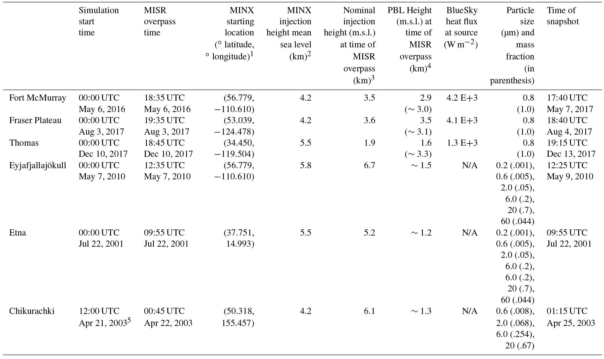
Volcano and wildfire plumes are initialized differently in the nominal HYSPLIT operation. Wildfire injection height is calculated dynamically throughout the simulation with a fire heat flux derived from an analysis of output data from the United States Forest Service BlueSky fire emissions model (https://www.airfire.org/bluesky, last access: 8 November 2018) and local meteorological conditions, whereas volcano injection height is generally input based on external observations. Between four and six particle sizes can be assumed for each volcano case, based on reporting from the Volcanic Ash Advisory Center (VAAC) responsible for region in which the eruption occurred. Each particle size makes up a portion of the total plume mass as defined by the particle size distribution from the VAAC report. Volcanic ash particle size distribution options are discussed in more detail in Leadbetter and Hort (2011), and the values for the cases considered in the current paper are listed in Table 1. Wildfire cases have only one assumed particle size in the nominal HYSPLIT process.
The following sections elaborate upon the nominal and MINX initialization procedures.
2.2.1 Volcano plume simulations
In order to create the nominal and MISR-initialized simulations, we followed the procedure specified for the VAAC Operational Dispersion Model Configuration (https://www.wmo.int/aemp/sites/default/files/VAAC_Modelling_OperationalModelConfiguration-March2016_v3.pdf, last access: 8 November 2018). Unlike the operational HYSPLIT set up, our “nominal” runs used MINX-derived source locations and source elevations. Operationally, eruption information from the Smithsonian Global Volcanism program (GVP) is used to determine source location and elevation. We chose instead to use the location and elevation from MINX, due to its high resolution and ability for the user to determine the exact location of the eruption. However, in practice there was little difference between the GVP-listed and MINX-derived source locations. Also, unlike the operational system, we used constant injection heights, determined by the MISR-estimated plume height at the specific time of the relevant satellite overpass for the MINX cases, and constant plume height as derived from the VAAC advisory nearest in time to the overpass for the nominal volcano cases. In the operational setting, injection height estimates are generally updated with each new forecast (e.g., every 6 h), and the operational simulations are designed to take advantage of these updated heights. For both the nominal and MINX simulations, each is set up as a line source from the vent to the maximum height of the plume, so it is assumed to have uniform mass distribution from the source to the injection peak. Injection peak was no further from the source than 50 km for wildfire plumes and 150 km for volcanic plumes. If observed further downwind, the maximum heights showed little difference from the injection height reported closer to the source, so subsequent advective plume rise is unlikely to affect our interpretation of the results.
For the MISR-initialized simulations, the injection heights are determined as the maximum heights obtained from the MINX histogram of plume contrast-element elevations at MISR overpass time. The MINX injection heights, nominal injection heights, and boundary layer heights obtained from near-coincident meteorological soundings, are given in Table 1. Unlike the VAAC injection-height observations, the uncertainty in the MINX digitizations can be quantified, and for the red-channel retrievals used in the current study, it is only around 250 m. Injection height, whether from MINX or the nominal configuration, is used to initialize the HYSPLIT simulations, after which the representation of dynamics and meteorological fields considered by the model account for advection, convection, and dispersion of aerosols.
To better isolate the impact of injection height on downwind plume dispersion, the MINX-constrained runs were configured exactly the same as the nominal runs, except for this variable. All other aspects of the simulation are determined by the VAAC reports and are defined in the operational configuration document cited above, including horizontal concentration-output grid spacing, particle size distribution (PSD), particle density, number of particle types, deposition settings, maximum altitude of the model, etc. As the values for these parameters reported by different VAACs can vary, our simulations aimed to match the configuration of the VAAC region in which the eruption occurred. The only exception is Chikurachki, which was set up with the Washington–Anchorage rather than the Tokyo VAAC configuration, due to its proximity to the Washington–Anchorage VAAC border and the fact that Washington–Anchorage uses HYSPLIT for their operational simulations.
As these simulations are meant to recreate short-to-medium range air quality forecasts for recent eruptions, we initialize the plume heights for the nominal cases based on VAAC advisories, if available, or the GVP (https://volcano.si.edu/, last access: 8 November 2018) otherwise. The VAAC observations are likely to be released first and be the best initial estimates for operational simulations. VAAC advisories that occurred closest to the time of the MISR overpass were used. The VAAC plume-height estimates are derived from ground-based or aircraft-based visible observations, from radar measurements, or from thermal infrared satellite soundings. In addition to the observational techniques used, plume height estimation can be determined based on an empirical relationship between plume height and mass eruption rate, in the rare case that there are no direct observations available (Mastin et al., 2009). All these methods, especially visible observations, come with notable uncertainties. A comparison between volcanic plume height from pilot reports, MINX heights, and ground-based plume-height assessments for volcanoes on the Kamchatka peninsula concluded that pilot reports were subject to the greatest uncertainties (Flower and Kahn, 2017). Radar-return heights generally skew toward the highest particle-rich part of the plume, satellite-based infrared retrievals sometimes must be corrected for thermal disequilibrium effects or sampling envelopes that include some signal from the surface below, and visual observations tend to encounter difficulties tracking the highest parts of plumes that are ash poor (Mastin et al., 2009).
As all three volcanic eruptions covered in this study occurred outside North America, the use of global meteorological data was required. Therefore, we were limited by the resolution at which global forecast models were archived during the time period of these eruptions. The coarseness of the meteorological data introduces some additional uncertainty into these simulations.
The Global Data Assimilation System (GDAS) 1.0∘ meteorological fields were chosen for the Eyjafjallajökull eruption case, and Final (FNL) Operational Global Analysis 1.0∘ meteorological data was used for eruptions that occurred before 2007. The data sets can be found in HYSPLIT-compatible formats on the NOAA Air Resources Laboratory (ARL) meteorological data archive website (https://www.ready.noaa.gov/archives.php, last access: 8 November 2018). The GDAS system is used by the National Center for Environmental Prediction (NCEP) Global Forecast System (GFS) model to place observations into a gridded model space for the purpose of starting, or initializing, weather forecasts with observed data (https://www.ncdc.noaa.gov/data-access/model-data/model-datasets/global-data-assimilation-system-gdas, last access: 8 November 2018). The FNL product is made with the same model NCEP used in the GFS, but the FNLs are prepared about an hour after the GFS is initialized, so more observational data can be applied (NCEP, 2000).
In summary, this work evaluates specifically the effect that initializing the HYSPLIT model with observed MINX plume heights has on the downwind dispersion of the modeled plumes.
2.2.2 Wildfire plume simulations
For wildfires, the model configurations are based on NOAA's Smoke Forecasting System (SFS) operational HYSPLIT simulations defined in Rolph et al. (2009). The meteorological data fields used when that document was written was hourly, 12 km horizontal resolution North American Mesoscale – Weather Research and Forecasting (NAM-WRF) fields. More recently, special high-resolution nested grids were added to the weather forecasting models in regions with active major fires to further increase the resolution. However, the present study focuses on large-scale plume dispersion over longer simulation periods, 96 h vs. the operational 72 h. As such, we used more skillful but lower-resolution GDAS 0.5∘ meteorological data. In a comparison of major numerical weather prediction models, it was found that the NAM was consistently the least skillful in short range forecasts of mean sea level pressure, and was subject to more error on the US West Coast, which is where all of our wildfire simulations take place (Wedam et al., 2009). Although higher resolution meteorological fields like the NAM12 are able to resolve smaller-scale features such as sea breezes and complex terrain, we found that the advantages of higher spatial resolution were compensated by lower model predictive skill, leaving the overall results of the study independent of the meteorological fields chosen. A comparison of simulations performed with both the GDAS 0.5∘ and NAM12 km fields can be found in the Thomas fire analysis in Sect. 3.3 below.
As in standard HYSPLIT operational runs, smoke plume-rise is calculated within the model based on the atmospheric stability, wind speed (both from the meteorological data), friction velocity, and a model-input heat flux from the BlueSky model, as described in Sect. 2.2 above. In addition to providing heat flux, the BlueSky model is used to estimate the emission rate of particulate matter less than 2.5 µm in diameter (PM2.5). The injection height calculated nominally by the model is given in the HYSPLIT “MESSAGE” file, which provides a diagnostic output of plume rise emission height and co-located mixed layer height above ground level (a.g.l.) at every hour of the simulation. In the nominal case, the injection height is dynamically varied throughout the simulation based on variations in heat release and atmospheric conditions, and the emissions at any time during the simulation are released at the model-estimated final plume rise at that time and location in the model.
The plume height of the MISR-initialized cases is determined through the MINX digitization and as with the volcano cases, is defined as a line source from the fire elevation to maximum plume height. In the MISR-initialized simulations, this maximum plume height is kept constant throughout the simulation, at the value determined at the specific time of the MISR overpass, which occurs on Day 1 of the simulation. As it is unrealistic for the injection height to remain at the same height for the entirety of the simulation, a vertical line source from the ground to this constant maximum height is used in the MISR-initialized case. This creates mass release in the MINX-initiated cases at levels between the surface and injection layer, accounting to some extent for lower-elevation injection with diurnal boundary layer expansion and contraction and other atmospheric profile changes. The particle properties assumed for both nominal and MINX simulations are the nominal HYSPLIT values: spherical particles with an average diameter of 0.8 µm and a density of 2 g cm−3, identical to the operational product (Rolph et al., 2009). Where the operational configuration and ours differ is in the source locations, as they are defined by MISR instead of MODIS/GOES, and the duration of the simulations, which are extended from 72 to 96 h, to provide a more comprehensive view of the effects of a more accurate injection height. The fire simulations are typically set to output average concentrations in one layer from 0 to 5 km above ground level. Although smoke plumes rarely exceed the 5 km level, the cases in the present study include some extreme fires that regularly do. So an additional difference between our nominal simulations and the operational system is that our model runs are set to output average concentrations in one layer from 0 to 10 km above ground level.
2.2.3 General configuration
In order to evaluate the atmospheric transport and dispersion predictions in the HYSPLIT simulations, we use the MODIS 3 km resolution Level 2 AOD data set (MOD04_3K and MYD04_3K for Terra and Aqua MODIS, respectively; https://ladsweb.modaps.eosdis.nasa.gov, last access: 8 November 2018) and accompanying MODIS visible imagery. To assess the ability of the model to simulate plume evolution, we output column mass concentration snapshots from HYSPLIT at the time of MODIS overpass for each day of the simulations, averaged from 0 to 10 km m.s.l. to obtain a total column average concentration, and compare with the MODIS total column optical depth. To create comparable products, each run is performed from the beginning of the event until 96 h later, outputting a plot coincident with every MODIS Terra overpass, or MODIS Aqua if a Terra overpass is unavailable. We plot each nominal and MISR-initialized HYSPLIT column mass concentration in arbitrary mass concentration units, as discussed in the next section.

Figure 2Fort McMurray wildfire smoke plume evolution. (a) Day 2 sampling of the HYSPLIT 96 h simulations that began on 6 May 2016, for 0–10 km, vertically integrated, qualitative smoke plume concentration based on MISR–MINX height initialization. Black outline indicates edges of visible smoke from satellite imagery and the black star indicates source location Panel(b) is the same as (a), but using the nominal HYSPLIT height initialization. (c) MISR-nominal initialization, qualitative smoke plume vertically integrated concentration differences. (d) MODIS true-color image acquired on 7 May 2016. Red outline matches black outline from panels (a), (b), and (c) but is red for visibility.
2.3 Evaluation
MODIS AOD is a column-integrated quantity, so evaluation of the plume dispersion simulations with these data is two-dimensional. To analyze the results of this study, we associate high-AOD regions from MODIS with areas where column mass integrated between 0 and 10 km elevation (i.e., the column mass concentration) is high, as determined by HYSPLIT. We test this assumption by comparing the spatial contours of HYSPLIT column mass concentration with the MODIS AOD maps (Supplement Fig. S1), by visual inspection. We then compare the conclusions drawn from the HYSPLIT concentration contour vs. MODIS AOD analysis with MODIS true color imagery, to identify any apparent spatial distribution differences and to associate smoke or volcanic aerosol opacity in the imagery with column concentration levels. The levels are represented by the colored hexagons in Fig. 2a and b, where the color represents concentration level and the hexagon represents a HYSPLIT output grid cell. Hexagons were used to better mesh adjoining grid points for the purposes of these plots. The mass concentration in each output grid cell is summed and assigned to a bin corresponding to the concentration. The bin values indicate relative mass concentration, at intervals increasing by half an order of magnitude, based on the simulations. The bin scale itself reports relative concentration values ranging from 0 (no mass) to 6 (most mass, assessed on an absolute scale of visibility), in intervals of 1. For example, a value that falls within the “Very High” range is placed into bin 6. A value corresponding to the “Haze” range is placed into bin 3. The same mass concentration scale is used for all cases in this study. We adopted this approach to avoid over-interpreting the data – mass concentration differences within a bin are unlikely to be significant, whereas we have much more confidence in the relative differences indicated by results falling into different bins. The HYSPLIT output grid cells are 0.25∘ latitude by 0.25∘ longitude for the wildfire cases. For the volcanic cases, the horizontal resolution varies by VAAC, as reported in the WMO documentation. We adjust the HYSPLIT grid to match the VAAC resolution.
Figure 2a and b present a snapshot at hour ∼42 of the 96 h HYSPLIT simulations of 0–10 km, vertically integrated, qualitative smoke plume concentrations for the Fort McMurray wildfire, beginning 6 May 2016. All daily snapshot samplings of the model simulations from each case are available in the Supplement. The fuchsia and dark blue levels denote places where particles were present but where the AOD is expected to be too low for the smoke or ash to be visible in the MODIS imagery. The cyan level denotes smoke or ash that is either not visible or slightly visible (haze), but should still have moderate optical depth values. The green level indicates where smoke should be easily visible from the satellite imagery and should have moderately high optical depth values. The orange level is where aerosol column concentrations are high and corresponding optical depth values should be very high, with patches of missing data where the AOD is too high for MODIS to observe to the surface. The red level represents the highest column concentrations of aerosols in the simulation, and should have no optical depth data because the smoke or ash would be too thick for MODIS AOD retrievals.
The difference plot (Fig. 2c) uses the same scale for all cases and is based on the difference between the mass concentration bins assigned to each output grid cell by the nominal- vs. MISR-initialized simulations. The dark blue contour represents much higher column concentrations predicted in the nominal than the MISR-initialized simulation, and has a value of −4 or lower. The cyan contour represents slightly higher column concentrations forecasted for the nominal than the MISR-initialized simulation, and has a value of −2 or −3. The white contour represents column concentrations predicted to be very similar in the two simulations, having values of −1, 0, or 1. The orange and red contours represent output grid cells where the column mass concentration is predicted to be slightly higher (2 or 3) or significantly higher (4 or more), respectively, in the MISR-initialized simulation than the nominal one. For example, a grid cell in the nominal simulation assigned to the “Very High” bin will have a value of 6. That same grid cell in the MISR-initialized simulation might be assigned to the “Visible” bin with a value of 4. Therefore the “MISR – Nominal Difference” value for that cell would be a −2 (“Nominal Slight”).
When assessing simulated atmospheric transport model performance, we compare the edges of the visible plumes in the satellite imagery with the qualitative green, cyan, or higher column mass concentration levels in the corresponding HYSPLIT images. In areas of cloud interference, as observed in the visible imagery, it is not possible to verify whether the aerosol concentrations determined by the model correspond to observation, unless the smoke or ash is above the cloud layer. Also, this verification method utilizes total column mass concentration average and total column AOD, so, as mentioned above, it does not assess vertical plume structure, which is beyond the scope of the current work.
One factor that determines the impact of the injection height on plume dispersion is whether the injection height is above the PBL. As wind speed and direction are generally different within vs. above the PBL, a model simulation is much more likely to approximate observations if the assumed injection height is on the correct side of this boundary. Based on MISR stereo retrievals, Kahn et al. (2008) found that about 18 % of wildfires in the boreal forest regions of Alaska and western Canada injected smoke above the PBL, and Val Martin et al. (2010), found that overall, approximately 4 %–12 % of wildfire plumes in North America inject above the boundary layer into the free troposphere. Whether a plume is injected above the PBL depends primarily on the dynamical heat flux produced by the fire, the ambient atmospheric stability structure, and the amount of entrainment of ambient air into the rising plume that occurs (Kahn et al., 2007). The time-of-day is a related factor, due to diurnal boundary layer expansion and contraction. The PBL tends to be well mixed, and usually grows deeper with solar heating during the day. The inversion at the top of the PBL helps confine smoke and other pollutants within its boundary; late in the day, as solar heating diminishes, the PBL typically collapses toward the surface. Winds within the PBL tend to show distinct differences from the more predictable and often stronger winds aloft, due to interactions between the boundary layer winds and the surface. In many cases, low-altitude wildfire injection heights were represented well in the nominal model, and resulted in very similar simulations to the MISR-initialized simulations. For the purposes of this study, we have chosen some cases that are very similar and some that show larger differences, to indicate the scope of the impact injection height has on HYSPLIT. Model snapshots taken on each day of each 4-day simulation are available in Supplement.
We now compare in detail the performance of HYSPLIT downwind, for three fire and three volcanic plume cases initialized using MISR–MINX plume injection height and with the nominal model value.
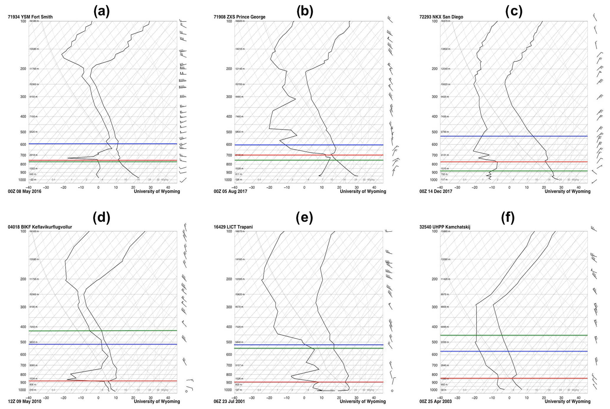
Figure 3Atmospheric soundings at each of the nearest airports at the closest time to the snapshot for each case. The vertical axis is atmospheric pressure in mb on a log scale and the horizontal axis is temperature in ∘C. Horizontal lines indicate approximate elevation in m, isotherms are indicated as light grey lines from lower left to upper right, and those generally trending toward the upper left are dry adiabats. The rightmost dark black line shows the temperature sounding, and the one to the left represents the dew point profile. Wind speeds and directions are indicated by the barbs on the right side of each plot. The red line marks the planetary boundary layer, the blue line marks the injection height of the MISR-initialized simulation, and the green line marks the injection height of the nominal simulation at the hour of the snapshot. (a) Fort McMurray, 8 May 2016, at 00Z: pbl ∼2.5 km, MISR-initialized =4.2 km, nominal ∼2.4 km. (b) Fraser Plateau, 5 August 2017, at 00Z: pbl ∼3.1 km, MISR-initialized =4.2 km, nominal ∼2.7 km. (c) Thomas fire, 14 December 2017, at 00Z: pbl ∼3.1 km, MISR-initialized =5.5 km, nominal ∼1.9 km. (d) Eyjafjallajökull, 9 May 2010, at 12Z: pbl ∼1.2 km, MISR-initialized =5.8 km, nominal =6.7 km. (e) Etna, 23 July 2001, at 06Z: pbl ∼1 km, MISR-initialized =5.5 km, nominal =5.2 km. (f) Chikurachki, 25 April 2003, at 00Z: pbl ∼1.3 km, MISR-initialized =4.2 km, nominal =6.1 km.
3.1 Fort McMurray fire plume, May 2016
Of the 4 days for the Fort McMurray wildfire simulation, 7 May 2016 (Fig. 2) best displays the differences between the nominal and MISR-initialized simulations. On the first simulated day of the event, MINX injection heights were above the PBL, based on both the atmospheric sounding from the nearby YSM airport and the GDAS meteorological fields included in Table 1. The nominal plume rise at the time of MISR overpass was also determined to be above the PBL based on the GDAS and the sounding. Of all the wildfire cases studied, the nominal plume rise calculation for the Fort McMurray simulation also seemed to perform best relative to the plume rise observed by MISR. However, as the simulation continues, the nominal injection height varies based on the HYSPLIT model, and begins to diverge from the MINX value acquired on Day 1; differences develop in the simulations. The model injection height, PBL height, and wind speeds for Day 2 of the Fort McMurray simulation are shown in Fig. 3a for the sounding on 8 May 2016 (00:00 UTC) at Fort Smith, just north of Fort McMurray. The PBL depth is discernable on the sounding by the inversion in temperature and rapid relative humidity decrease at about 2.5 km. The injection height as determined by MISR was 4.2 km m.s.l. and was set nominally by HYSPLIT at about 2.4 km m.s.l. at the time the MISR snapshot was acquired. Unlike the injection height calculated by HYSPLIT on Day 1 of the simulation, the nominal injection height for Day 2 is below the PBL. From the differences in wind speed and direction at each level it is clear that poor injection height initialization will affect the accuracy of downwind air quality forecasts. Figure 2 shows the MISR-initialized and nominal simulations, MISR-initialized minus nominal difference plots, and MODIS true color imagery for the Fort McMurray wildfires on Day 2 of the simulations. The MODIS AOD is shown in Fig. S1a. Although the overall plume shapes, trajectories, and concentrations seem relatively similar, the difference plot reveals a significant deviation (Fig. 2c). In the northwestern corner of the outlined portion of the plume, the MISR-initialized simulation displays higher aerosol concentrations than does the nominal one. When compared to the MODIS optical depth and visible imagery, the northern portion of this feature is covered in clouds, so the aerosol is obscured in the satellite data, but the southern portion is visible. The visible image has an optically thick, well-defined plume in the same area as the MISR-initialized case, favoring the MISR simulation, and the AOD map shows very high aerosol concentrations. There are missing data points in the AOD map, further indicating that concentrations are very high, as there is a lack of cloud cover in the visible imagery.
In this case, we see a large difference in injection height arise by the second day of the simulation. The nominal injection height is located below the PBL whereas the MISR-initialized injection height is still above the PBL. We then observe a large difference in the simulated aerosol concentration for this northwestern feature; it shows better agreement with the MISR-initialized simulation than the nominal simulation based on the MODIS visible imagery and AOD.
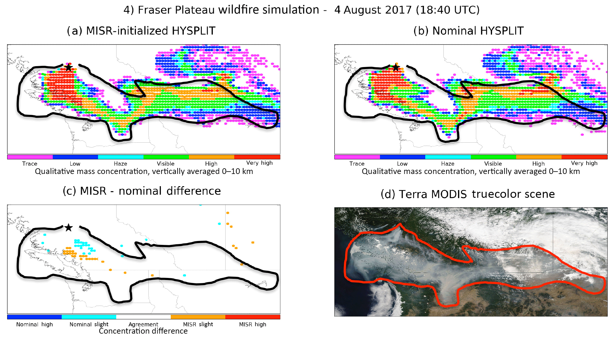
Figure 4Same as Fig. 2, but for the Fraser Plateau Fire plume on 4 August 2017. (a–b) Day 2 samplings of HYSPLIT 96 h simulations that began on 3 August 2017, and (c) Day 2 difference plot. (d) MODIS true-color image acquired on 4 August 2017.
3.2 Fraser Plateau fire plume, August 2017
The Fraser Plateau case study (Fig. 4) is an example of the impact that meteorology and a relatively uniform wind profile can have on dispersion simulations. Table 1 shows an approximate 0.6 km plume rise underestimation in the nominal case at the time of the MISR overpass. By Day 2 of the simulation, the nominal plume is at 1.5 km a.s.l., and the difference had grown to approximately 1.4 km, although the actual injection height may have decreased as well. The sounding from ZXS Prince George on Day 2 of the simulation (Fig. 3b) shows the PBL to be at approximately 3.1 km, indicating the MINX injection height is above the PBL, and nominal injection height is below the PBL. In the case studies examined here, simulations in disagreement about injection height being above or below the PBL generally show differences in plume dispersion that substantially exceed the uncertainty in the measurements. However, based on Fig. 3b, the winds above the PBL are also fairly consistent with those below the inversion in this case, generally coming from the north around 10–15 knots (5–8 m s−1). In addition, about half the plumes simulated in the MISR-initialized case are injected below the 3.1 km PBL. Even though some plumes exceed the PBL, the wind shear differences are not significant enough to create large discrepancies, as we saw in the Fort McMurray case. Differences in plume dispersion between the nominal HYSPLIT and MINX-initialized simulations shown in Fig. 4c do not exceed “slight,” and there are very few such differences. Higher smoke concentrations coincide with visible smoke in the true color images, and MODIS AOD mapping is also consistent. This is true for hour 42.3 of the simulation, where visible smoke appears in the southeastern corner of the MODIS image. Even this far into the simulation and approximately 1000 km downwind, visible smoke can be seen entering the Montana region, in agreement with the visible imagery, highlighting the accuracy of both the MISR-initialized and nominal simulations for this case.
Although large differences in injection height between the two simulations tend to yield different results, as shown here, this is not the only factor involved. As the root cause of differences between the simulations is the changing meteorology above and below the PBL, similar meteorological conditions will produce similar results even if the injection heights are separated by the PBL.
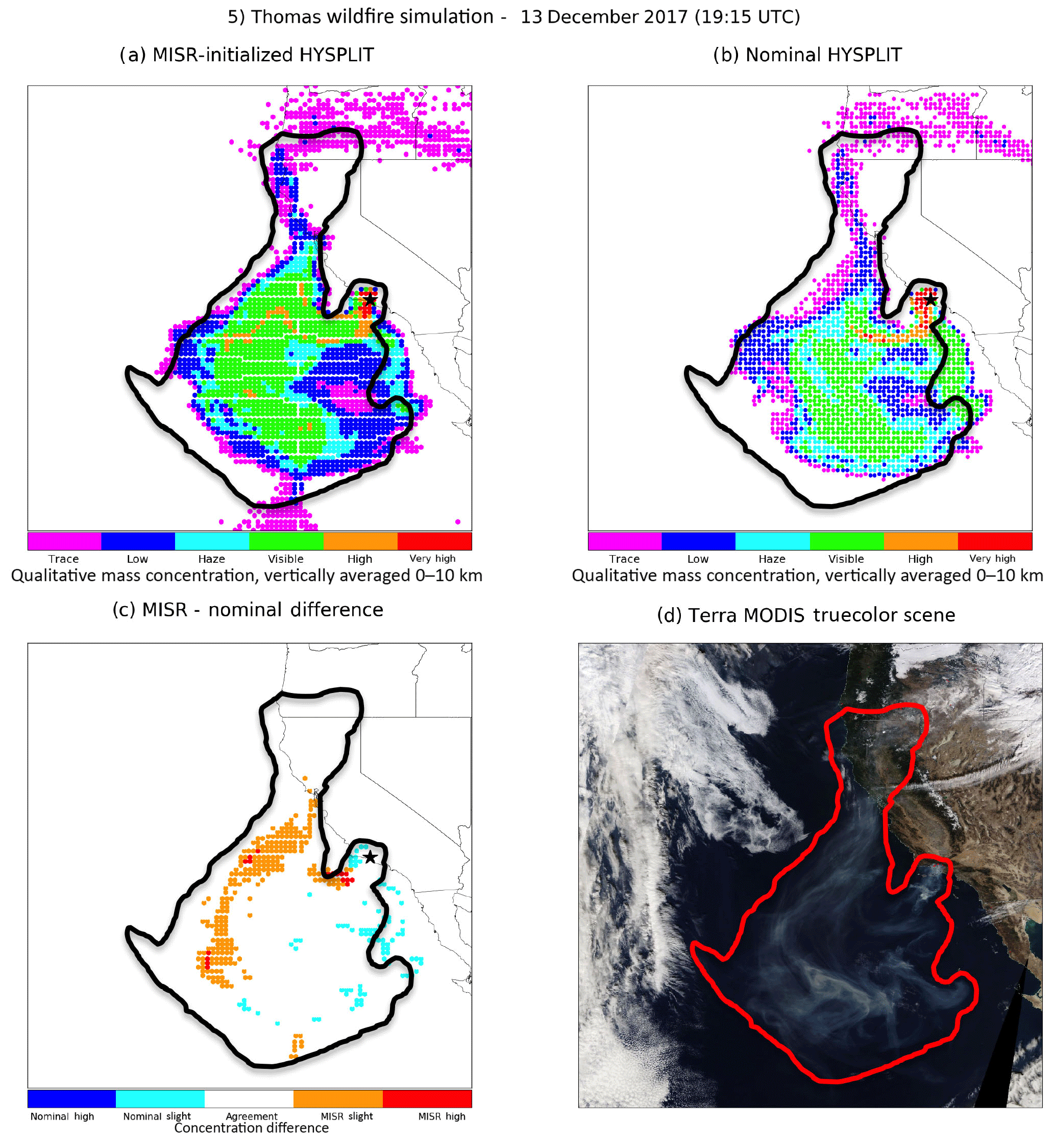
Figure 5Same as Fig. 2, but for the Thomas fire plume, on 13 December 2017. (a–b) Day 4 samplings of HYSPLIT 96 h simulations run with the GDAS 0.5∘ meteorology, beginning on 10 December 2017, and (c) Day 4 difference plot. (d) MODIS true-color image acquired on 13 December 2017.
3.3 Thomas fire plume, December 2017
The Thomas fire was an ideal case for testing the differences between meteorological fields having different spatial resolutions. Theoretically, the NAM12 higher resolution meteorological data used in the current comparison would be more effective at resolving the fairly complex terrain and mesoscale meteorological processes such as sea breezes that might operate here. However, we understand that the NAM lacks the skill the ECMWF and GFS models can achieve, even at coarser resolution. Figures 5 and 6 show Day 4 of the Thomas fire simulation run with GDAS 0.5∘ and NAM12 meteorological data, respectively. The overall plume dispersion is quite similar between the GDAS and NAM simulations. In both cases, the nominal simulations are slightly higher, e.g., along the eastern and southern edges of the visible plume, and on the western edge of the visible plume the MISR-initialized simulation is significantly higher. Figures 5c and 6c highlight the differences between the GDAS and NAM simulations. The locations where the differences occur are almost identical, but the nominal vs. MINX differences are much more prominent in the NAM12 plot (Fig. 6c). As such, even in a location with complex terrain and mesoscale meteorological processes affecting the simulations, the plume dispersion simulations can be similar, with qualitative results independent of the meteorological data spatial resolution, but quantitatively, the differences can be significant.
In contrast to the Fraser Plateau fire, there were significant differences in wind speeds (and direction) with altitude for the Thomas fire. There was also a large difference in the nominal and MINX injection heights; on Day 1, 1.9 and 5.5 km mean sea level (m.s.l.), respectively (Table 1). Although these values apply to the higher of the two plumes simulated, even the lower plume reached an elevation of 4.4 km m.s.l., indicating a difference of approximately 2.5–3.6 km between the nominal and MINX injection heights at MISR overpass time. Figure 5 shows the snapshots of each simulation on 13 December at 19:15 UTC, which is over 90 h after the initialization of this simulation. Although both simulations perform well, especially considering how many hours after initialization this snapshot is taken, it is clear that the MISR-initialized simulation performed better, based on the difference plot in Fig. 5c. Whereas the nominal simulation predicts slightly higher smoke concentrations near the southern edges of the outlined visible plume, it also predicts higher concentrations outside the visible plume that do not coincide with the contemporaneous MODIS visible imagery or AOD mapping. In addition, the MISR-initialized simulation predicts much higher smoke concentrations in the western portion of the visible plume outline, where the AOD is high and the visible imagery shows a dense band of smoke extending to the north or northeast.
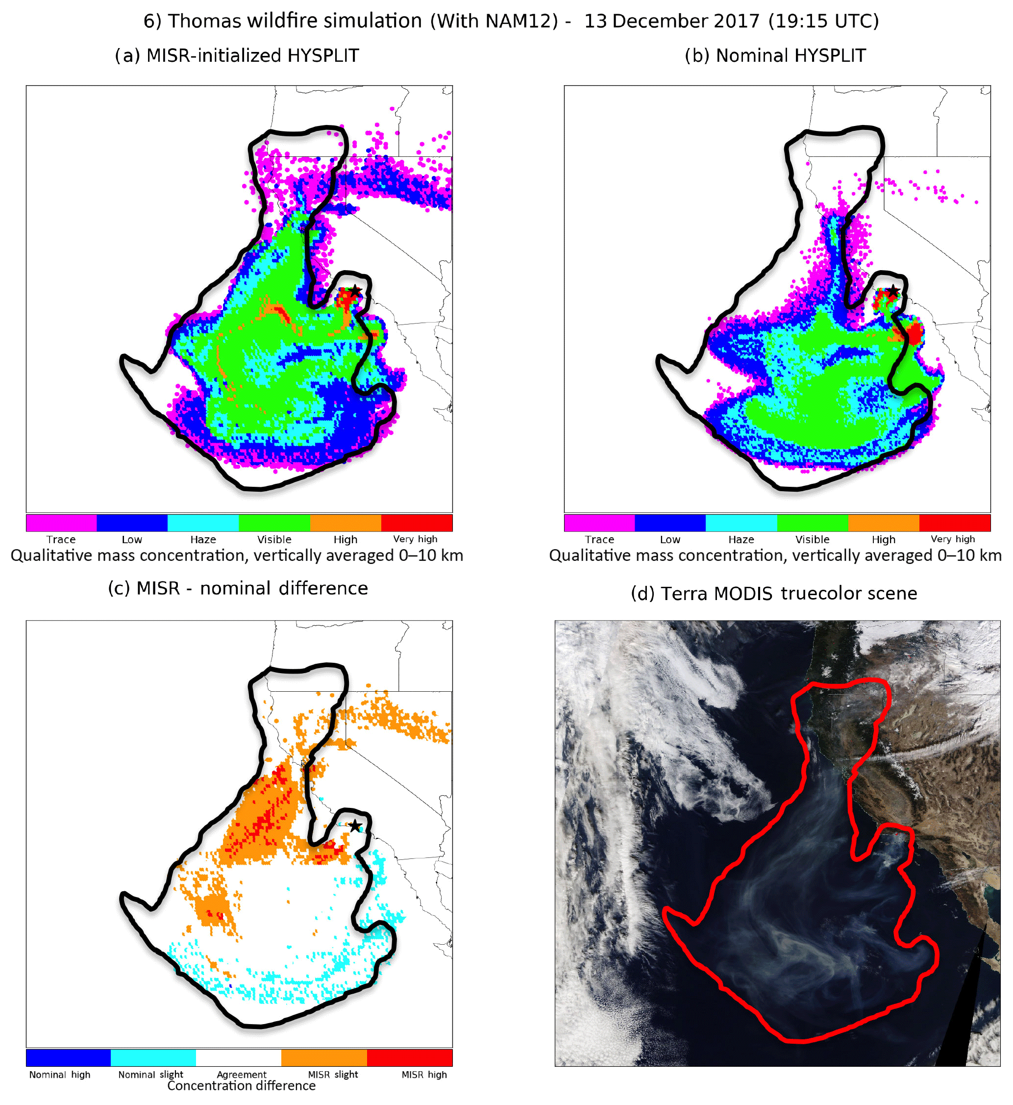
Figure 6Same as Fig. 2, but for the Thomas fire plume, on 13 December 2017, using NAM12 km meteorological data. (a–b) Day 4 samplings of HYSPLIT 96 h simulations run with the NAM12 meteorology, beginning on 10 December 2017, and (c) Day 4 difference plot. (d) MODIS true-color image acquired on 13 December 2017.
The stronger advection that likely carried the smoke further in the westerly direction can be attributed to the stronger winds aloft shown in Fig. 3c. At the MINX injection height, winds are out of the northeast at approximately 13–15 m s−1 (25–30 knots). The nominally calculated injection height is located around 1.9 km m.s.l., where the winds are light and variable around 2.6 m s−1 (5 knots).
This case reinforces many of the conclusions drawn from the Fort McMurray simulation. Large differences in nominal vs. MISR-initialized injection heights create very different results, favoring the MISR-initialized case when compared to MODIS validation. Unlike the Fraser Plateau case, differences in meteorology above and below the PBL were significant and yielded significantly different simulations.

Figure 7Same as Fig. 2, but for the Eyjafjallajökull volcanic eruption plume, on 9 May 2010. (a–b) Day 3 samplings of HYSPLIT 96 h simulations that began on 7 May 2010, and (c) Day 3 difference plot. (d) MODIS true-color image acquired on 9 May 2010.
3.4 Eyjafjallajökull volcanic eruption plume, May 2010
For the volcanic cases, it is common for the injection heights of each plume to overshoot the height of the boundary layer due to the explosive nature of many such events. The nominal HYSPLIT injection heights are constrained by external data, so in many cases, the differences between the injection heights obtained from the VAAC and the corresponding MINX value are not large. There are exceptions, however, e.g., Flower and Kahn (2017). In addition, the meteorological conditions tend to be less variable with elevation within the free troposphere than between the free troposphere and the PBL, so detecting differences between the nominal and MISR-initialized HYSPLIT simulations can be more difficult than for wildfires. The VAAC advisory for the first day of this eruption reported plume heights at 6.7 km near MISR overpass time, whereas the MINX-derived injection height had a maximum height of about 5.8 km. Although 0.9 km is a significant difference in injection height, Fig. 3d shows winds at these two levels within 2.6 m s−1 (5 knots) of each other and are in nearly the same northwesterly direction. This can account for the nearly identical dispersion snapshots in Fig. 7.
As indicated by comparison with the MODIS visible imagery and AOD, both simulations reproduce the eruption well. The dispersion of the main plume extending from the vent is captured with high precision, and is constrained within the visible plume outline on each figure. Near-source concentrations are also high, as seen in the true color image. Both simulations predicted a higher-concentration patch of ash on the eastern end of the laterally moving portion of the plume, which is apparent in the visible imagery (circled portion) as well. Although they both slightly misplace this portion of the plume, this snapshot was taken over 60 h after initialization. The presence and general location of such a small feature helps to emphasize the accuracy of HYSPLIT when initialized with accurate injection heights.
Large volcanic eruptions tend to inject ash well above the PBL, which means that simulated plumes are exposed to the generally less variable meteorology of the free troposphere. Due to this factor, differences between the simulations tend to be small, and can be difficult to discern.
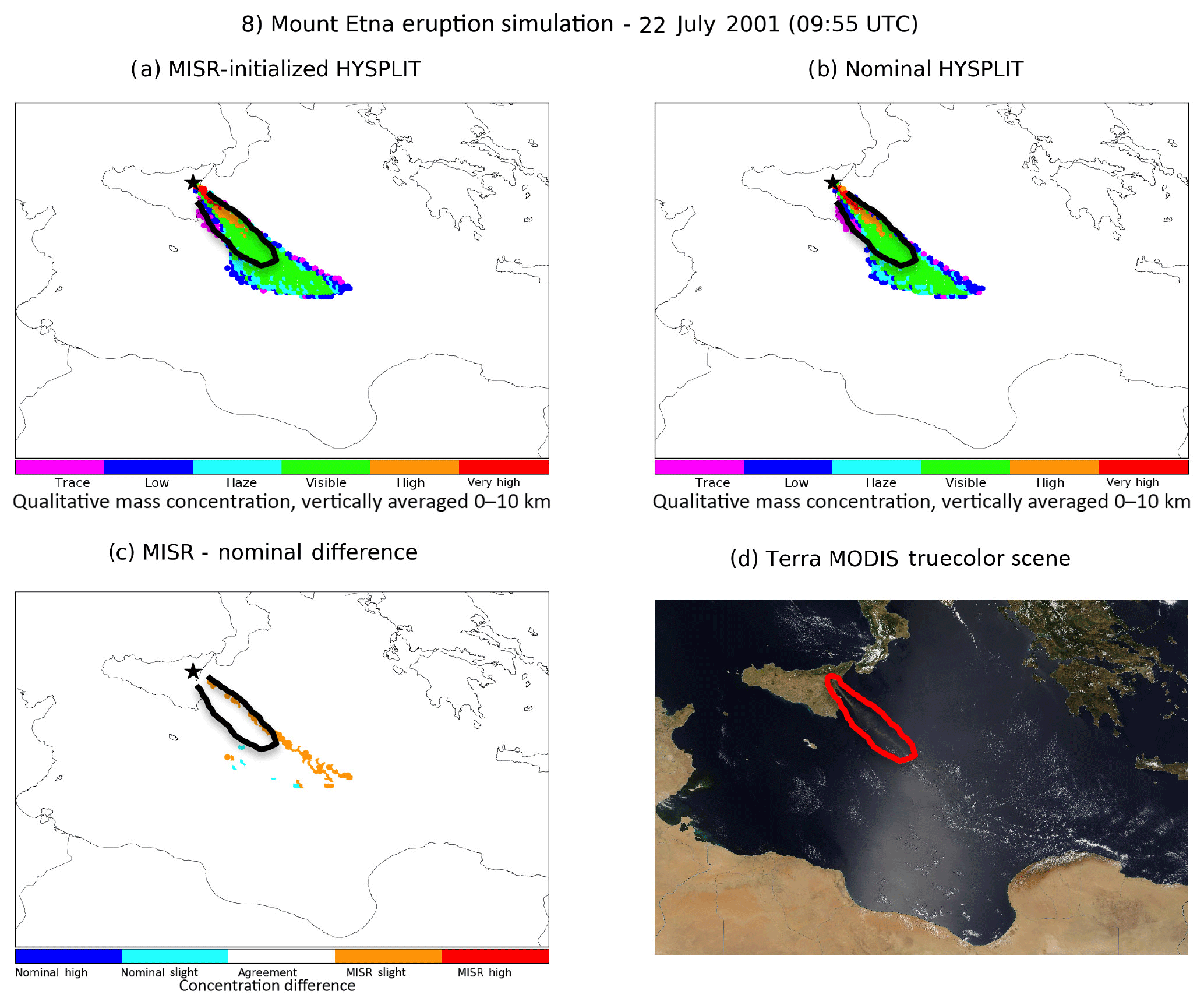
Figure 8Same as Fig. 2, but for the Mount Etna volcanic eruption plume, on 22 July 2001. (a–b) Day 1 samplings of HYSPLIT 96 h simulations that began on 22 July 2001, (c) and Day 1 difference plot. (d) MODIS true-color image acquired on 22 July 2001.
3.5 Mount Etna volcanic eruption plume, July 2001
The distinctions between the nominal and MISR-initialized cases for the Mount Etna eruption are subtle compared to the wildfire cases discussed above. The observed PBL height is about 1 km in the sounding (Fig. 3e). The MINX injection height is at about 5.5 km, and the nominal HYSPLIT injection height equals approximately 5.2 km. As expected, with injection height initializations this similar the plume dispersion is almost identical. Differences between the simulations are minimal, detailed in the difference plot (Fig. 8c), and do not exceed the “slight” category. However, the MISR-initialized simulation does indicate the presence of slightly higher ash concentrations on the northeastern portion of the plume and the nominal indicates slightly higher ash concentrations on the southwestern portion of the plume. Neither of these features can be verified due to the sun glint affecting these areas in the MODIS imagery, but the near-source portions of the plume in both simulations have high correlations with the plume outlines the visible imagery.
The Mount Etna case is another example of small simulation differences due to fairly uniform meteorological conditions in the free troposphere. This case also reinforces the assertion that very similar injection heights produce similar results. The differences between the nominal and MISR-initialized injection heights were only approximately 0.3 km, so it is likely that meteorological conditions at these altitudes were similar.
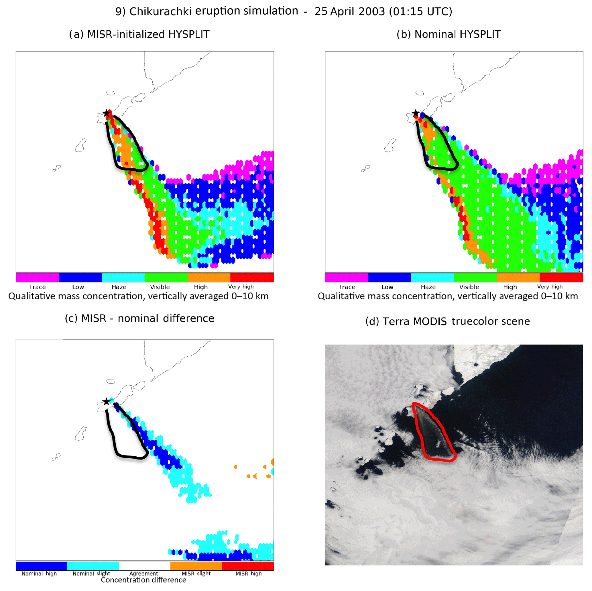
Figure 9Same as Fig. 2, but for the Chikurachki volcanic eruption plume, on 25 April 2003. (a–b) Day 4 samplings of HYSPLIT 96 h simulations that began on 21 April 2003, and (c) Day 4 difference plot. (d) MODIS true-color image acquired on 25 April 2003.
3.6 Chikurachki volcanic eruption plume, April 2003
The final case of this study was the Chikurachki eruption of April 2003 (Fig. 9) in the Kuril Islands, southwest of the Kamchatka Peninsula. The sounding shown in Figs. 3f and 9 maps take place on the final day of the simulation, approximately 84 h after HYSPLIT initialization. For this case, the MINX injection height is 4.2 km and the nominal value is about 6.1 km. As indicated in Fig. 3f, the PBL height near this overpass time was around 1.3 km, so both injection heights are within the free troposphere. However, significant differences are observed in vertical wind shear between these altitudes. Figure 3f shows winds about 15.4 m s−1 (30 knots) faster at 6 km than at 4 km, and the wind direction is more westerly aloft as well. Differences in the wind vectors suggest that the near-source concentrations would be lower in the nominal than the MINX-initialized simulation, because the plume particles would be advected away more quickly; a more easterly trajectory for the nominal simulation will alter the dispersion accordingly.
Both plots in Fig. 9 support these predictions. In addition, the plume shape is more accurately modeled in the MISR-initialized simulation. When comparing the plume outlines in the visible imagery, the nominal case has a significantly wider visible plume than the MISR-initialized plume, which captures the visible portion almost exactly. Clearly the western plume is better represented by the MISR-initialized simulation. But note that the eastern branch is also captured by the MISR-initialized simulation (green “visible plume” region in Fig. 9a) in the right location based on the MODIS image of Fig. 9d, and the corresponding black outline in Fig. 9a. What the MISR-initialized simulation seems to miss is the sub-visible part between the east and west plumes; this is likely a consequence of the coarse contouring between “very high,” “high,” and “visible” optical thickness. The nominal simulation exceeds the MISR one only outside the black outline, where no plume was observed. It is also important to note that concentration differences at scales this small are difficult to evaluate because of the coarse resolution of the global meteorological data. This is why we have placed more emphasis on the overall plume shape and trajectory for this case than the small-scale differences in ash concentration.
These retrievals demonstrate how inaccuracies the in altitude used to initialize the model can significantly diminish the accuracy of the downwind plume dispersion simulation, even when the aerosol is emitted into the free troposphere. In this case, the observed discrepancies include the near-source aerosol concentration, the plume trajectory, and plume shape in the portion of the plume that can be verified in the cloud-free imagery.
The Chikurachki case further emphasizes the fact that simulations can provide very different results when a large injection-height difference exists. It also demonstrates that, even in volcanic eruption cases with meteorological conditions in the free troposphere, conditions can still be significantly different at different altitudes. As the MISR-initialized case showcases better agreement with the visible imagery and AOD, it is reasonable to say that the more accurate injection height was key to providing the improved result.
In this paper, we present a detailed analysis of how injection-height initialization impacts the downwind plume simulations by the HYSPLIT model, for six well-defined wildfire smoke and volcanic aerosol plumes. In many cases, plume dispersion is accurately represented in both the nominal and MISR-initialized simulations. However, discrepancies do occur between the nominal and MISR injection altitude. Based on the analysis presented here, initializing HYSPLIT simulations with injection height determined via MINX can improve the dispersion dynamics of wildfire and volcanic aerosol plumes. The differences tend to be most pronounced when the injection estimates fall on either side of the boundary between the PBL and the free troposphere. Even if both simulations are initialized above the PBL, as in most volcanic cases, the VAAC advisories used to initialize HYSPLIT in the analysis shown here tend to overestimate the height; wind shear common in the free troposphere produces discrepancies in downwind plume dispersion nevertheless. (Note also that the VAAC data used to initialize the nominal HYSPLIT process are obtained primarily from MODIS suborbital observations, and we selected cases from among those volcanoes that have the best ground monitoring, whereas many other volcanoes around the globe are not monitored at all by surface or aircraft instrumentation.)
Obtaining accurate downwind simulation results has important ramifications for aviation safety and air quality policy. For example, though observations have shown that particulate matter has decreased and related air quality improved overall in the United States, this is not true in the wildfire-prone Northwestern states (McClure and Jaffe, 2018), and is not the case for much of the rest of the world. If a state can prove that violations of the National Ambient Air Quality Standards (NAAQS) are due to natural activity (e.g., biomass burning) they may submit an exceptional events demonstration under the 2016 Exceptional Events Rule in order to avoid penalties assessed by the Environmental Protection Agency. These demonstrations often rely heavily on the use of HYSPLIT (e.g., Washoe County Health District, 2016) which necessitates the best possible representation of plume dispersion within the model framework.
The HYSPLIT wildfire simulations also appear to be more sensitive to variations in injection height than volcanic simulations. This is likely because wildfires frequently inject smoke near the PBL – free-troposphere boundary, where small changes in elevation can produce large differences in ambient wind speed and direction. Model estimation of wildfire plume-rise from first principles remains a challenging scientific problem (e.g., Val Martin et al., 2012). Yet, we note that MISR provides global coverage only about once per week on average, and the trade-off between initializing a simulation with more accurate MINX injection heights several days prior to a time of interest, vs. using less accurate injection heights derived by a model closer to the time of interest, would depend on the particulars of the case involved. In future work, we hope to evaluate the wildfire plume-rise algorithms in HYSPLIT by comparison with plume-rise estimates from MINX in more detail. If the evaluation shows that improvements can be made, we hope to develop new approaches to more accurately simulate plume rise.
As assessing plume rise specifically was not the main goal of the current research, the use of half-degree meteorological data was deemed sufficient to assess the large-scale plume dispersion analyzed here. However, finer spatial resolution, non-hydrostatic meteorological fields will be important for evaluating plume rise on smaller scales, especially in the complex terrain environments where many wildfires typically occur. As there are many variables in addition to plume injection height that affect the accuracy of HYSPLIT simulations, future work might include constraining model simulations with other information provided by satellite instruments. For example, MISR aerosol type (Kahn et al., 2001; Limbacher and Kahn, 2014) could be used to initialize HYSPLIT instead of the operational particle characteristics from the SFS and VAACs. In addition, other observations, such as space-based CALIPSO lidar downwind aerosol layer heights and ground-based sensor AOD and particle properties, can help increase confidence in long-range smoke or volcanic aerosol dispersion forecasting.
Another next step would be to quantitatively evaluate the aerosol column mass concentration values and ground-level concentrations in HYSPLIT simulation results. More research into mass extinction coefficient values and their relationship to aerosol optical depth is needed to address this issue (e.g., Kahn et al., 2017), as this quantity determines the relationship between column-integrated AOD and aerosol column mass concentration. If the values can be reliably converted, quantitative analysis becomes possible, expanding upon the qualitative results shown in this study. Yet, we have demonstrated qualitatively the influence aerosol injection height uncertainty can exert over simulation results. Further, we have highlighted the importance of further efforts to reduce the uncertainty in these estimates for real-world emissions situations, and have also demonstrated that the use of MINX injection heights, when available, can improve downwind dispersion forecasts in the HYSPLIT model.
All MISR data are archived and are publicly available at the Atmospheric Sciences Data Center, NASA Langley Research Center (http://eosweb.larc.nasa.gov, NASA ASDC, 2018).
The supplement related to this article is available online at: https://doi.org/10.5194/amt-11-6289-2018-supplement.
Conceptualization: CJV, RAK, TC; Methodology: CJV, RB, RAK, TC; Digitizing Plumes: CJV and RB; Analysis: CJV, RB, RAK, TC; Writing, Reviewing, and Editing: CJV and RAK; Supervision: RAK, TC.
The authors declare that they have no conflict of interest.
We thank Mark Cohen and Alice Crawford from the NOAA Air Resources Lab for
providing assistance with the HYSPLIT simulations presented here. Mark Cohen also
participated in reviewing early versions of the manuscript to ensure
accurate representation of the HYSPLIT model simulations. The work of Charles J. Vernon and Ryan Bolt is supported in part by a grant from the NASA Earth
Science Applications program under Lawrence Friedl.
Charles J. Vernon is also funded in part
by Timothy Canty, and in part by a grant from the NASA Atmospheric Composition Program
under Robert Eckman. The work of Ralph A. Kahn is supported in part by the NASA
Climate and Radiation Research and Analysis Program under Hal Maring and the
NASA Atmospheric Composition Modeling and Analysis Program under Robert Eckman.
The Terra/MODIS and Aqua/MODIS MOD04_3K and MYD04_3K datasets were acquired from the Level-1 and Atmosphere Archive and Distribution
System (LAADS) Distributed Active Archive Center (DAAC), located in the Goddard Space Flight Center in Greenbelt,
Maryland (https://ladsweb.nascom.nasa.gov/,
last access: 16 November 2018).
We acknowledge the use of imagery from the NASA Worldview application (https://worldview.earthdata.nasa.gov/,
last access: 16 November 2018)
operated by the NASA Goddard Space Flight Center Earth Science Data and Information System (ESDIS) project.
We would like to acknowledge the use of the atmospheric sounding archive from the University of
Wyoming College of Engineering (http://weather.uwyo.edu/upperair/sounding.html,
last access: 16 November 2018).
Edited by: Thomas Eck
Reviewed by: two anonymous referees
Colarco, P. R., Schoeberl, M. R., Doddridge, B. G., Marufu, L. T., Torres, O., and Welton, E. J.: Transport of smoke from Canadian forest fires to the surface near Washington, D.C.: Injection height, entrainment, and optical properties, J. Geophys. Res., 109, 2156–2202, https://doi.org/10.1029/2003JD004248, 2004.
Crawford, A. M., Stunder, B. J. B., Ngan, F., and Pavolonis, M. J.: Initializing HYSPLIT with satellite observations of volcanic ash: A case study of the 2008 Kasatochi eruption, J. Geophys. Res.-Atmos., 121, 10786–10803, 2016.
Diner, D. J., Beckert, J. C., Reilly, T. H., Bruegge, C. J., Conel, J. E., Kahn, R. A., Martonchik, J. V., Ackerman, T. P., Davies, R., Gerstl, S. A. W., Gordon, H. R., Muller, J. P., Myneni, R. B., Sellers, P. J., Pinty, B., and Verstraete, M. M.: Multi-angle Imaging SpectroRadiometer (MISR) instrument description and experiment overview, IEEE T. Geosci. Remote, 36, 1072–1087, https://doi.org/10.1109/36.700992, 1998.
Flower, V. and Kahn, R.A.: Assessing the altitude and dispersion of volcanic plumes using MISR multi-angle imaging: Sixteen years of volcanic activity in the Kamchatka Peninsula, Russia, J. Volcanol. Geoth. Res., 337, 1–15, 2017.
Forouzanfar, M. H. et al.: Global, regional, and national comparative risk assessment of 79 behavioural, environmental and occupational, and metabolic risks or clusters of risks in 188 countries, 1990–2013: a systematic analysis for the Global Burden of Disease Study 2013, Lancet, 386, 2287–232387, https://doi.org/10.1016/S0140-6736(15)00128-2, 2015.
Kahn, R., Li, W., Moroney, C., Diner, D., Martonchik, J., and Fishbean, E.: Aerosol source plume physical characteristics from space-based multiangle imaging, J. Geophys. Res., 112, D11205, https://doi.org/10.1029/2006JD007647, 2007.
Kahn, R. A. and Limbacher, J.: Eyjafjallajökull volcano plume particle-type characterization from space-based multi-angle imaging, Atmos. Chem. Phys., 12, 9459–9477, https://doi.org/10.5194/acp-12-9459-2012, 2012.
Kahn, R. A., Banerjee, P., and McDonald, D.: The Sensitivity of Multiangle Imaging to Natural Mixtures of Aerosols Over Ocean, J. Geophys. Res., 106, 18219–18238, 2001.
Kahn, R. A., Chen, Y., Nelson, D., Leung, F., Li, Q., Diner, D., and Logan, J.: Wild Smoke Injection Heights: Two Perspectives From Space, Geophys. Res. Lett., 35, L04809, https://doi.org/10.1029/2007GL032165, 2008.
Kahn, R. A., Berkoff, T., Brock, C., Chen, G., Ferrare, R., Ghan, S., Hansico, T., Hegg, D., Martins, J. V., McNaughton, C. S., Murphy, D. M., Ogren, J. A., Penner, J. E., Pilewskie, P., Seinfeld, J., and Worsnop, D.: SAM-CAAM: A Concept for Acquiring Systematic Aircraft Measurements to Characterize Aerosol Air Masses, B. Am. Meteorol. Soc., 98, 2215–2228, https://doi.org/10.1175/BAMS-D-16-0003.1, 2017.
Leadbetter, S. J. and Hort, M. C.: Volcanic ash hazard climatology for an eruption of Hekla Volcano, Iceland, J. Volcanol. Geoth. Res., 199, 230–241, https://doi.org/10.1016/j.jvolgeores.2010.11.016, 2011.
Limbacher, J. A. and Kahn, R. A.: MISR research-aerosol-algorithm refinements for dark water retrievals, Atmos. Meas. Tech., 7, 3989–4007, https://doi.org/10.5194/amt-7-3989-2014, 2014.
Mastin, L. G., Guffanti, M., Servranckx, R., Webley, P., Barsotti, S., Dean, K., Durant, A., Ewert, J. W., Neri, A., Rose, W. I., Schneider, D., Siebert, L., Stunder, B., Swanson, G., Tupper, A., Volentik, A., and Waythomas, C. F.: A multidisciplinary effort to assign realistic source parameters to models of volcanic ash-cloud transport and dispersion during eruptions, J. Volcanol. Geoth. Res., 186, 10–21, https://doi.org/10.1016/j.jvolgeores.2009.01.008, 2009.
McClure, C. D. and Jaffe, D. A.: US particulate matter air quality improves except in wildfire-prone areas, P. Natl. Acad. Sci. USA, 115, 7901–7906, https://doi.org/10.1073/pnas.1804353115, 2018.
Moroney, C., Davies, R., and Muller, J.-P.: MISR stereoscopic image matchers: Techniques and results, IEEE T. Geosci. Remote, 40, 1547–1559, 2002.
Muller, J.-P., Mandanayake, A., Moroney, C., Davies, R., Diner, D. J., and Paradise, S.: Operational retrieval of cloud-top heights using MISR data, IEEE T. Geosci. Remote, 40, 1532–1546, 2002.
NASA ASDC: Atmospheric Science Data Center, available at: http://eosweb.larc.nasa.gov, last accesss: 15 November 2018.
National Centers for Environmental Prediction/National Weather Service/NOAA/U.S. Department of Commerce: NCEP FNL Operational Model Global Tropospheric Analyses, continuing from July 1999, Research Data Archive at the National Center for Atmospheric Research, Computational and Information Systems Laboratory, Boulder, Colo, (Updated daily), https://doi.org/10.5065/D6M043C6, 2000.
NCEP GDAS: Global Data Assimilation System (GDAS), https://www.ncdc.noaa.gov/data-access/model-data/model-datasets/global-data-assimilation-system-gdas, last access: 15 November 2018.
Nelson, D., Yang, C., Kahn, R., Diner, D., and Mazzoni, D.: Example Applications of the MISR INteractive EXplorer (MINX) Software Tool to Wildfire Smoke Plume Analyses, Proc. SPIE., 7089, 708909, https://doi.org/10.1117/12.795087, 2008.
Nelson, D., Garay, M., Kahn, R., and Dunst, B.: Stereoscopic Height and Wind Retrievals for Aerosol Plumes with the MISR INteractive eXplorer (MINX), Remote Sens., 5, 4593–4628, https://doi.org/10.3390/rs5094593, 2013.
Rolph, G. D., Draxler, R. R., Stein, A. F., Taylor, A., Ruminski, M. G., Kondragunta, S., Zeng, J., Huang, H., Manikin, G., McQueen, J. T., and Davidson, J. T.: Description and Verification of the NOAA Smoke Forecasting System: The 2007 Fire Season, Weather Forecast., 24, 361–378, https://doi.org/10.1175/2008WAF2222165.1, 2009.
Stein, A., Draxler, R., Rolph, G., Stunder, J., and Cohen, M.: NOAA's HYSPLIT Atmospheric Transport and Dispersion Modeling System, B. Am. Meteorol. Soc., 96, 2059–2077, https://doi.org/10.1175/BAMS-D-14-00110.1, 2015.
Stein, A. F., Rolph, G. D., Draxler, R. R., Stunder, B., and Ruminski, M.: Verification of the NOAA Smoke Forecasting System: Model Sensitivity to the Injection Height, Weather Forecast., 24, 379–394, 2009.
Stunder, B. J. B., Heffter, J. L., and Draxler, R. R.: Airborne volcanic ash forecast area reliability, Weather Forecast., 22, 1132–1139, 2007.
Val Martin, M., Kahn, R., Logan, J., Paugam, R., Wooster, M., and Ichoku, C.: Space-based observational constraints for 1-D fire smoke plume-rise models, J. Geophys. Res, 117, D22204, https://doi.org/10.1029/2012JD018370, 2012.
Washoe County Health District, Air Quality Management Division: Exceptional Events Demonstration for 2015 Ozone Exceedance in Washoe County from the 2015 California Wildfires, https://www.epa.gov/sites/production/files/2017-06/documents/washoe2015wildfiredemonstration_withaddendum.pdf (last access: July 2018), 2016.
Walter, C., Freitas, S. R., Kottmeier, C., Kraut, I., Rieger, D., Vogel, H., and Vogel, B.: The importance of plume rise on the concentrations and atmospheric impacts of biomass burning aerosol, Atmos. Chem. Phys., 16, 9201–9219, https://doi.org/10.5194/acp-16-9201-2016, 2016.
Wedam, G., McMurdie, L., and Mass, C.: Comparison of Model Forecast Skill of Sea Level Pressure along the East and West Coasts of the United States, Weather Forecast., 24, 843–854, https://doi.org/10.1175/2008WAF2222161.1, 2009.