the Creative Commons Attribution 4.0 License.
the Creative Commons Attribution 4.0 License.
 | 02 Feb 2018
Ground-based FTIR retrievals of SF6 on Reunion Island
Bavo Langerock
Corinne Vigouroux
Pucai Wang
Christian Hermans
Gabriele Stiller
Kaley A. Walker
Geoff Dutton
Emmanuel Mahieu
Martine De Mazière
SF6 total columns were successfully retrieved from FTIR (Fourier transform infrared) measurements (Saint Denis and Maïdo) on Reunion Island (21∘ S, 55∘ E) between 2004 and 2016 using the SFIT4 algorithm: the retrieval strategy and the error budget were presented. The FTIR SF6 retrieval has independent information in only one individual layer, covering the whole of the troposphere and the lower stratosphere. The trend in SF6 was analysed based on the FTIR-retrieved dry-air column-averaged mole fractions () on Reunion Island, the in situ measurements at America Samoa (SMO) and the collocated satellite measurements (Michelson Interferometer for Passive Atmospheric Sounding, MIPAS, and Atmospheric Chemistry Experiment Fourier Transform Spectrometer, ACE-FTS) in the southern tropics. The SF6 annual growth rate from FTIR retrievals is 0.265±0.013 pptv year−1 for 2004–2016, which is slightly weaker than that from the SMO in situ measurements (0.285±0.002 pptv year−1) for the same time period. The SF6 trend in the troposphere from MIPAS and ACE-FTS observations is also close to the ones from the FTIR retrievals and the SMO in situ measurements.


Sulfur hexafluoride (SF6) is very stable in the atmosphere and is well-mixed and one of the most potent greenhouse gases listed in the 1997 Kyoto protocol linked to the United Nations Framework Convention on Climate Change (UNFCCC). It has an extremely long lifetime of 850 years (Ray et al., 2017) with global warming potential for a 100-year time horizon of 23 700 (relative to CO2) (Kovács et al., 2017). Since SF6 is a very stable trace gas in the atmosphere and its annual growth rate seems relatively constant during the last two decades (Hall et al., 2011), it is usually applied to calculate the age of air (Patra et al., 1997; Engel, 2002; Patra et al., 2009; Stiller et al., 2012; Haenel et al., 2015).
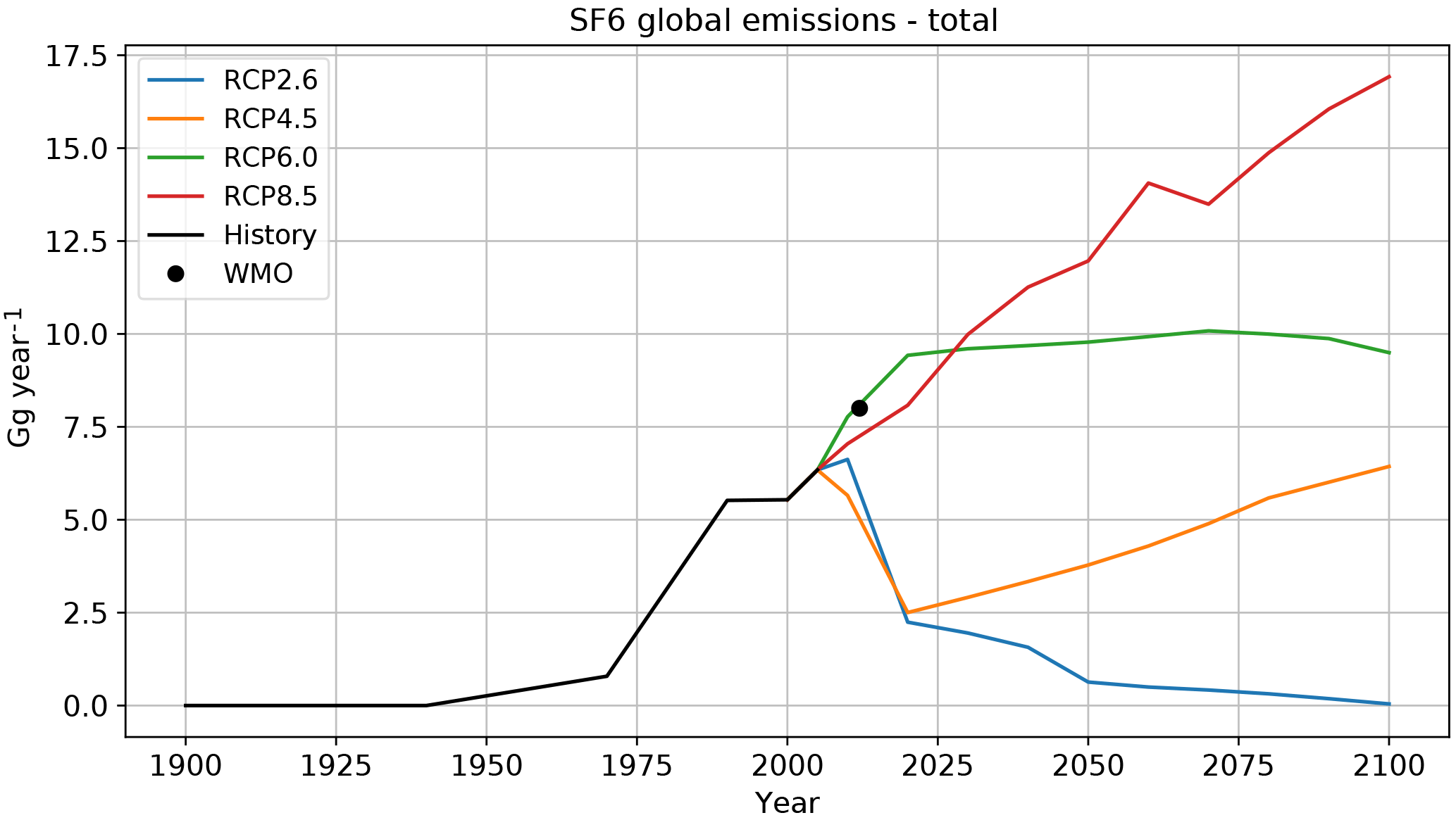
Figure 1Time series of historical and projected global SF6 emissions. Historical data cover 1900–2005 (black), and projections for the 2005–2100 time period correspond to four RCP scenarios with 2.6, 4.5, 6.0 and 8.5 W m−2 radiative forcing in 2100 relative to pre-industrial values (Moss et al., 2010). The black dot is the annual growth of SF6 in 2012 according to the WMO report (WMO, 2014).
SF6 is emitted from anthropogenic sources at the Earth's surface, mainly from the chemical industry, such as in production of electrical insulators and semi-conductors, and magnesium manufacturing. The mole fraction of SF6 in the atmosphere has increased in recent years and the globally averaged near-surface SF6 volume mixing ratio (VMR) has reached up to 7.6 pptv (parts per trillion by volume), with an annual increase of 0.3 pptv year−1 in 2012 (WMO, 2014). Figure 1 shows the SF6 historical global emissions in 1900–2005 (Schultz et al., 2008; Mieville et al., 2010). Emissions of SF6 started in the 1940s and have been increasing since then. Only during 1990–2000 the emissions almost remain constant. The most likely reason is that SF6 emissions decreased in developed countries between 1995 and 1998 but then increased again after 1998 (Levin et al., 2010; Rigby et al., 2010). The SF6 global total emissions in 2005 were 6.341 Gg year−1 (1 Gg=1000 t), which is about 8 times larger than that in 1970 (0.789 Gg year−1). Figure 1 also shows the predictions of SF6 global emissions for 2005–2100 according to four representative concentration pathway (RCP) scenarios with different radiative forcing values (2.6, 4.5, 6.0 and 8.5 W m−2) in 2100 relative to pre-industrial values (Moss et al., 2010). The RCP 6.0 and RCP 8.5 scenarios assume the emissions keep increasing until 2020 and 2100 respectively, while RCP 2.6 and RCP 4.5 scenarios assume that there will be a steep decrease after 2010. The predictions from these four scenarios are very different, so it is very important to monitor the abundance of SF6 in the atmosphere. The most recent Scientific Assessment of Ozone Depletion report (WMO, 2014) points out that the global emissions have amounted to 8.0 Gg year−1 in 2012, marked by a black dot in Fig. 1.
The Advanced Global Atmospheric Gases Experiment (AGAGE) gas chromatography–mass spectrometry (GC–MS) system has measured the SF6 concentration since 1973 (Rigby et al., 2010). The Halocarbons and other Atmospheric Trace Species Group (HATS) started SF6 sampling measurements at eight stations in 1995 and in situ measurements at six fixed sites in 1998 (Hall et al., 2011). The flask and in situ measurements show that the SF6 abundance in the atmosphere has been increasing since the 1970s (Maiss and Levin, 1994; Geller et al., 1997; Maiss and Brenninkmeijer, 1998; Moss et al., 2010). In recent decades, remote sensing techniques also contribute to monitoring SF6. Rinsland et al. (1990) used the spectra observed by the Atmospheric Trace Molecule Spectroscopy instrument (ATMOS) aboard the space shuttle, as part of the Spacelab 3 (SL3) payload, to retrieve SF6 concentrations in the upper troposphere and lower stratosphere. In addition, space-based sensors, such as the Atmospheric Chemistry Experiment Fourier Transform Spectrometer (ACE-FTS) (Bernath et al., 2005; Bernath, 2017) and the Michelson Interferometer for Passive Atmospheric Sounding (MIPAS) (Stiller et al., 2008), are applied to obtain an SF6 global distribution and trend. Zander et al. (1991) succeeded in monitoring the increasing total column of SF6 using the ground-based Fourier transform infrared spectrometer (FTIR) at Jungfraujoch (46.55∘ N, 7.98∘ E, 3.58 ). Later on, Rinsland et al. (2003) and Krieg et al. (2005) obtained the total columns of SF6 from the FTIR measurements at Kitt Peak (31.9∘ N, 111.6∘ W, 2.09 ) and Ny-Ålesund (78.91∘ N, 11.88∘ E, 0.02 ). They found that the mixing ratio of SF6 is continuously increasing and that the mean increases of SF6 are 0.31±0.08 pptv year−1 at Ny-Ålesund, 0.24±0.01 pptv year−1 at Jungfraujoch and 0.28±0.09 pptv year−1 at Kitt Peak from March 1993 to March 2002. In the latest Scientific Assessment of Ozone Depletion, the trends of SF6 from in situ measurements are consistent with the trends in the troposphere from remote sensing measurements (ACE-FTS, MIPAS and Jungfraujoch FTIR) (WMO, 2014).
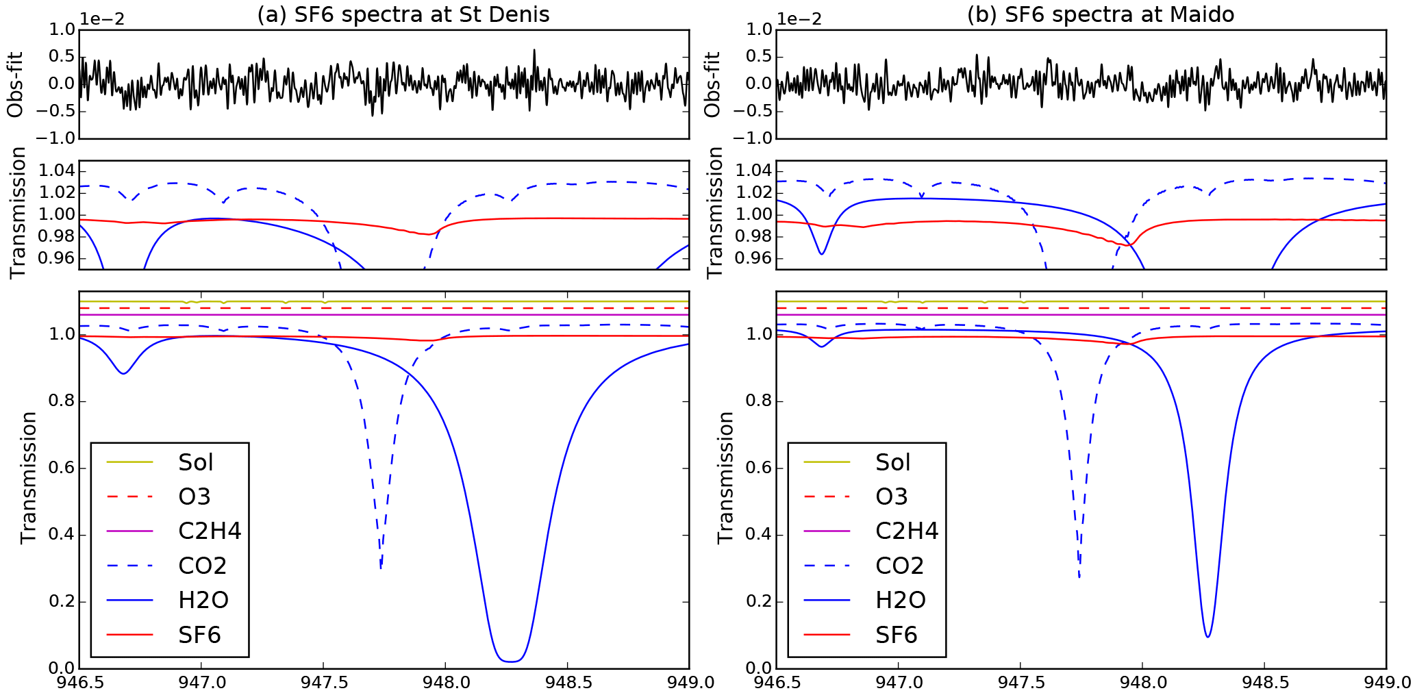
Figure 2The typical spectrum of SF6 retrieval microwindows (946.5–949.0 cm−1) at St Denis (a) and Maïdo (b). The bottom panels list the absorption contribution from each species. To clarify the absorption lines, the transmittance is shifted by 0.02 for each species and the solar (sol) line list. The middle panels only show the transmittance between 0.95 and 1.05 and identify the SF6 absorption line. The top panels show the transmittance residual (observed minus calculated).
The objective of this paper is to investigate the SF6 retrievals in the southern tropics based on the spectra observed by two FTIR spectrometers on Reunion Island (21∘ S, 55∘ E) from 2004 to 2016. In Sect. 2, SF6 retrievals are carried out with the well-established SFIT4 algorithm, which is upgraded from the radiative transfer and retrieval algorithm SFIT2 (Pougatchev et al., 1995; Hase et al., 2004) and widely used in the Network for the Detection of Atmospheric Composition Change Infrared Working Group (NDACC-IRWG) community. The FTIR SF6 retrieval strategy and the error budget are discussed in detail. In the following section, the trend in SF6 is analysed based on the FTIR retrievals, the HATS America Samoa (SMO) in situ measurements (14∘ S, 170∘ W, 77 ) and the collocated satellite measurements (MIPAS and ACE-FTS). Finally, conclusions are drawn in Sect. 4.
The Royal Belgian Institute for Space Aeronomy operates at two FTIR sites on Reunion Island. One is at Saint Denis (St Denis), close to the coast (20.90∘ S, 55.48∘ E; 85 m a.s.l.), and the other one is located at the Maïdo mountain site (21.07∘ S, 55.38∘ E; 2155 m a.s.l.). At present, both sites are equipped with a Bruker 125HR spectrometer, a precise solar-tracker system and an automatic weather station. The St Denis FTIR is dedicated to the near-infrared spectral region and has contributed to the Total Carbon Column Observing Network (TCCON) since September 2011, whereas the Maïdo FTIR is dedicated to the mid- to thermal infrared spectral region and has become an NDACC-IRWG instrument in March 2013. Before September 2011, a Bruker 120M instrument was operated at St Denis in the NDACC mid- to thermal infrared configuration. For detailed information about the two sites, please refer to Zhou et al. (2016) and the references therein.
The SF6 retrievals use the spectra in the thermal infrared range. Therefore, we select the spectra from the Bruker 120M at St Denis (2004–2011) and from the Bruker 125HR at Maïdo (2013–2016).
The spectra of 700–1400 cm−1 at St Denis and Maïdo are recorded with the same settings. Two maximum optical path differences (MOPDs) of 82 and 125 cm are operated to gather the interferogram of the direct solar radiation, and then the interferogram is transformed to a spectrum with the spectral resolutions of 0.010975 and 0.0072 cm−1 through a fast Fourier transform (FFT) algorithm. The HgCdTe (MCT) detector collects the spectrum and one specific interference filter is used to narrow the optical band to regions of interest in order to improve the signal-to-noise ratio (SNR).
2.1 Retrieval strategy
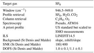
We used the SFIT4_v9.4.4 algorithm (Pougatchev et al., 1995) to retrieve information from the spectra: it simulates the spectrum observed by the ground-based FTIR and looks for the optimum state vector (the retrieved state) to minimise the residual between the simulated and the observed spectra. Table 1 lists the retrieval window, interfering gases, spectroscopic database, a priori profile, background parameters and SNR used in the SFIT4 algorithm for the SF6 retrieval at St Denis and Maïdo, together with the obtained degrees of freedom of signal (DOFS).
2.1.1 Retrieval window
The broad unresolved Q branch of the ν3 band of SF6, at 947.9 cm−1 (Varanasi et al., 1992), is always used to retrieve SF6 by remote sensing techniques. Zander et al. (1991) used 946.9–948.9 cm−1 for the FTIR retrieval at Jungfraujoch and Krieg et al. (2005) used 947.2–948.6 cm−1 for Kitt Peak and Ny-Ålesund FTIR retrievals. We also used the SF6 absorption line at 947.9 cm−1 and the retrieval window 946.5–949.0 cm−1 to perform the FTIR retrieval at Reunion Island. However, compared with the previous studies, our retrieval window contains an additional weak H2O absorption line at 946.68 cm−1. Since there is a strong H2O absorption line at 948.26 cm−1 and a strong CO2 line at 947.74 cm−1 (see Fig. 2), the SF6 is inevitably influenced by these two species, especially from H2O due to its larger variability in the atmosphere. A better fitting of H2O (with a smaller root mean square (rms) of the fitting residual) is obtained by the larger retrieval window. In addition, to minimise interference from H2O and CO2, their profiles are retrieved simultaneously with the SF6 profile.
2.1.2 Instrument line shape
In order to acquire the instrument line shape (ILS) and to verify the alignment of the instrument, daily HBr cell measurements are carried out automatically at both sites. The LINEFIT14.5 programme (Hase et al., 1999) is applied to obtain the modulation and phase parameters of the ILS, which are used as input to the SFIT4 algorithm. Note that we made a 3-order polynomial fitting from the LINEFIT outputs and then retrieved the polynomial parameters in SFIT4 algorithm for both modulation and phase.
2.1.3 Spectroscopy
The spectroscopy of SF6 was taken from the pseudo-line lists (http://mark4sun.jpl.nasa.gov/pseudo.html), and the spectroscopy of the other species was obtained from the ATM16 line lists (Toon, 2014). Pseudo-line lists were produced by Geoff Toon (NASA-JPL) by fitting all the laboratory spectra simultaneously, which includes mean intensities and effective lower state energies on a 0.005 cm−1 frequency grid. These artificial lines at arbitrary positions do not represent transitions of molecules. Instead, their line-widths and intensities are fitted to the laboratory spectra such that the pseudo-line lists allow to simulate the measured spectra.
2.1.4 A priori profile
To construct an a priori profile that is close to the true one, we used the US standard atmosphere (1976) SF6 (National Geophysical Data Center, 1992) as the shape of the a priori profile, and then scaled it with a factor of one to make the concentration of the lowest level equal to the annual mean of SMO measurements in 2009. The H2O a priori profile was derived from the 6-hourly NCEP reanalysis data. For the a priori profiles of the other interfering species (see Table 1), the mean of the Whole Atmosphere Community Climate Model (WACCM) version 6 monthly profiles between 1980 and 2020 were adopted.
2.1.5 Regularisation matrix
The a priori covariance matrix, together with the measurement noise covariance matrix, determine the weights of a priori knowledge and measurement information (Rodgers, 2000). The SNR were set to 180 and 400 at St Denis and Maïdo, respectively. In order to extract as much information as possible from the measurements and to avoid too many oscillations in the retrieved SF6 profiles, we used 30 and 14 % as the diagonal elements (the same value for all levels) to create the regularisation matrices at St Denis and Maïdo, respectively. The correlation width was set to 10.0 km. Note that the diagonal value of the regularisation matrix is a key parameter that balances the contribution from the measurement information and the a priori information, but does not represent the real variability of SF6 in the atmosphere.
2.1.6 Averaging kernel
Figure 3 shows the typical averaging kernel of the SF6 retrieval at Maïdo. The FTIR retrieval is sensitive to the altitude range from the surface to 20 km (the whole of the troposphere and lower stratosphere). The mean and standard deviations of the DOFS of the SF6 retrievals are 1.0±0.1 at St Denis and 1.1±0.1 at Maïdo, indicating that the SF6 retrievals have information content in only one individual layer (mainly 0–20 km) and have no profile information. That means the retrieved profiles are not reliable, and we should focus on the total column. In this study, the SF6 retrievals at St Denis were combined with Maïdo retrievals to extend the time coverage for the trend in Sect. 3. The DOFS at the two stations are very similar, and there is no observed trend in the time series of the DOFS.
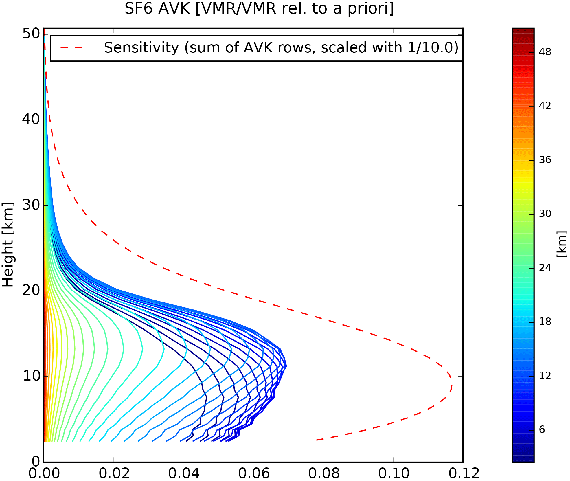
Figure 3The typical averaging kernel of SF6 retrieval at Maïdo. The solid lines represent the sensitivities at specific altitudes. The red dashed line is the sum of the rows of averaging kernels scaled by 0.1, indicating the vertical sensitivity.
2.2 Error budget
Based on the optimal estimation method (Rodgers, 2000), the difference between the retrieved state vector and the true state vector xt could be expressed as
where xa is the a priori state vector; A is the averaging kernel matrix, representing the sensitivity of the retrieved state vector to the true state vector; I is a unit matrix; Gy is the contribution matrix, representing the sensitivity of the retrieval to the measurement y; Kb is the weight function, representing the sensitivity of the forward model F(x,b) to the forward model parameters; b is the vector of forward model parameters that are not retrieved; bt is the vector of true forward model parameters; Δf is the forward model systematic uncertainty; εy is the measurement noise covariance matrix. Note that the state vector x, which is the vector of forward model parameters that are retrieved, is a higher-dimensional vector which consists of the target SF6 profile components, the concentration profiles for the interfering species (H2O, CO2) and other retrieval parameters (slope, ILS, etc.).
The error in the target SF6 profile is obtained by extracting the SF6 components from the vectorial equation in Eq. (1). The error in the retrieved SF6 profile then consists of the smoothing error , model parameter error GyKb(bt−b), forward model error GyΔf and measurement noise Gyεy. As the SFIT4 algorithm is well established and only the physics of the absorption is included in the transmission of radiation, the forward model error can be ignored.
Table 1The retrieval window, interfering gases, spectroscopic database, a priori profile, background parameters (slope and zshift) and SNR used in the SFIT4 algorithm for FTIR SF6 retrieval at St Denis and Maïdo, together with the achieved DOFS (mean and the standard deviation) of the retrievals.
The smoothing error, except for the uncertainty from SF6, also includes the uncertainties from the H2O profile, the CO2 profile, the C2H4 and O3 scaling factors and some other parameters (see Table 1), and is defined as the retrieval parameter error εre. Since the absorption lines of H2O and CO2 are very strong in the retrieval window, the εre is separated into three components.
where , , and are the matrices extracted from the full averaging kernel A by selecting the components Aij where the row index i runs over all SF6 components in the state vector x and the column index j runs over all SF6, H2O, CO2 and other components in state vector x. and , and , and , xt,others and xa,others are the true and a priori values of SF6, H2O, CO2 and other retrieval parameters.
Systematic and random components are considered to characterise the uncertainty of each parameter. For the smoothing error , we assumed that the systematic uncertainty of is 5 % relative to the a priori profile (). Then, the diagonal and off-diagonal values of the systematic part of are calculated as () and , respectively (von Clarmann, 2014). The random part of is constructed in the same way as the regularisation matrix but the diagonal elements were set to 30 % for both St Denis and Maïdo. For the measurement error Gyε, there is no systematic uncertainty and the random uncertainty is derived from the SNR.
For the εre, we mainly focus on the influence from H2O and CO2. The systematic and the random uncertainties of the H2O profile were derived from the bias and the standard deviation of the differences between the NCEP profiles and the balloon sondes. In general, the systematic uncertainty is about 5 % and the random uncertainty is about 10 % from surface to 10 km. The CO2 systematic uncertainty is assumed to be 5 % of the average of the WACCM monthly profiles, and the random uncertainty is the standard deviation of the WACCM monthly profiles from 1980 to 2020.
Table 2The systematic and random uncertainties for the FTIR-retrieved total column (%) at St Denis and Maïdo. σb are the relative systematic (random) uncertainties of the non-retrieved parameters (%). The “retrieval parameters” represents the “others” in Eq. (3). The SF6 spectroscopy uncertainty is from the pseudo-line database. When a relative uncertainty is smaller than 0.1 %, it is considered negligible and represented as “–”.
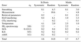
For the model parameter error GyKb(bt−b), we only show the significant parameters here, i.e. temperature, spectroscopy, solar zenith angle (SZA), ILS and zero level offset (zshift). The systematic and random uncertainties of the temperature profile were derived from the mean and the standard deviation of the differences between the NCEP profiles and the balloon sondes on Reunion Island in 2011. In general, the systematic bias is about 5 K below 10 km, 3 K between 10 and 15 km and 1 K above 15 km. The standard deviation is about 2–4 K in the troposphere and 5–10 K above tropopause height. The SF6 spectroscopy uncertainty is from the pseudo database: 2 % for the systematic part and zero for the random part. Values of 0.1 and 0.2 % were adopted for the systematic and random uncertainties of SZA according to the Pysolar package (one Python code to calculate the solar position http://pysolar.org/), while 5 and 1 % were adopted for both systematic and random uncertainties of the ILS parameters and zshift, respectively.
Table 2 lists the SF6 FTIR retrieval systematic and random uncertainties (%) at St Denis and Maïdo. The “retrieval parameters” in Table 2 represents the “others” in Eq. (3). The smoothing error, measurement error, H2O interference and temperature error at St Denis are much larger than those at Maïdo. In total, the retrieval systematic and random uncertainties (relative to the retrieved SF6 total column) are 4.6 and 14.0 % at St Denis and 3.7 and 6.7 % at Maïdo, respectively.
3.1 Data sets
3.1.1 SMO in situ measurements
Since 1998, a four channel gas chromatograph (CATS) system has been measuring the surface SF6 at the SMO site. Due to the high accuracy and precision, the CATS SF6 daily data from the NOAA ESRL halocarbon in situ measurement programme are considered to be a reference for comparison with the FTIR retrievals. Note that these are daily median data instead of daily means and are used to filter the higher outliers from local pollution. As there is an improvement in the instrument in June 2000, the standard deviation of 1-day measurements decreased from 0.2 to 0.4 to 0.02–0.04 pptv after the change (Hall et al., 2011).
3.1.2 MIPAS
MIPAS derived the global distributions of profiles of SF6 from limb observations between 2002 and 2012. MIPAS observed spectra in full spectral resolution (FR) mode (spectral resolution: 0.05 cm−1) and reduced resolution (RR) mode (spectral resolution: 0.121 cm−1) before and after January 2005. In this paper, we used the latest SF6 product with newly calibrated level 1b spectra (Haenel et al., 2015) to compare it with the FTIR retrievals and to make the SF6 trend analysis. The SF6 data used here are versions V5h_SF6_20 for the FR data product and V5r_SF6_222 and V5r_SF6_223 for the RR period. The MIPAS retrievals cover the upper troposphere (down to cloud top, or ∼6 km in cloud-free cases) and the stratosphere only (about 55 km; see Fig. 7). Since MIPAS single SF6 profiles are very noisy, we used the monthly means in the latitude band of 20–25∘ S.
3.1.3 ACE-FTS
Global distributions of SF6 are also monitored by ACE-FTS occultation measurements from 2004 (Boone et al., 2013). We used the ACE-FTS level 2 version 3.5 monthly data (2004–2013) from the ACE/SCISAT database, and only the measurements without any known issues (quality flag = 0) were selected (Sheese et al., 2015). The ACE-FTS data have been validated with MkIV balloon profiles (Velazco et al., 2011). Since ACE-FTS mainly look at the polar area, there are few measurements in the tropical zone. Geller et al. (1997) found that SF6 is well mixed throughout the Southern Hemisphere; therefore, we enlarged the latitude band for ACE-FTS measurements to 0–40∘ S to get a robust result. Similar to MIPAS measurements, ACE-FTS collects the spectra in the upper troposphere and stratosphere (about 10–30 km; see Fig. 7).
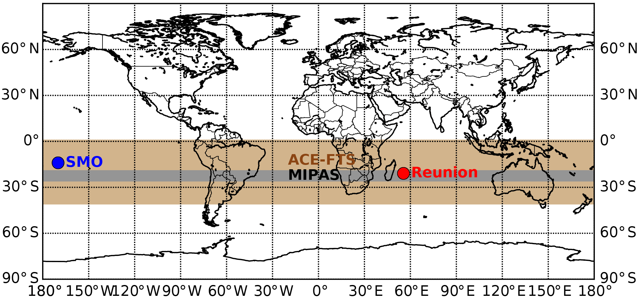
Figure 4The locations of the ground-based sites (Reunion Island and SMO) as well as the latitude bands covered by the satellites (MIPAS and ACE-FTS).
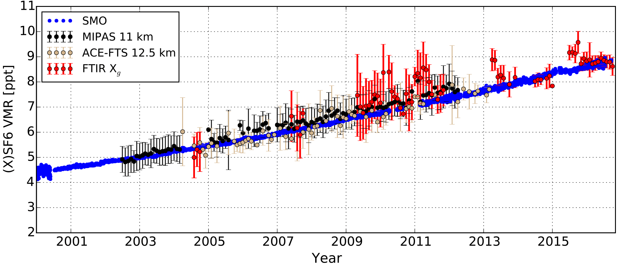
Figure 5Time series of SMO in situ SF6 daily median (blue), MIPAS SF6 monthly mean (20–25∘ S) at 11 km (black), ACE-FTS SF6 monthly mean (0–40∘ S) at 12.5 km and FTIR monthly mean at St Denis and Maïdo (red). For MIPAS, ACE-FTS and ground-based FTIR measurements, the error bar is the standard deviation within 1 month.
3.1.4 Ground-based FTIR
As the FTIR SF6 retrievals have only one layer of information, we applied the dry-air column-averaged SF6 () of FTIR measurements to quantitatively compare it with other data sets. is obtained by dividing the SF6 total column by the dry-air total column.
where and are the total columns of SF6 and dry air; Ps is the surface pressure; g is the acceleration of gravity depending on the latitude and altitude; and and are the molecular masses of H2O and dry air, respectively; is the total column of H2O from NCEP re-analysis data. The surface pressure is recorded with a Vaisala PTB210 sensor, with accuracy better than 0.1 hPa. The systematic uncertainty of H2O in the troposphere is about 5 %, and the on Reunion Island is about 1–2 % of the TCair. As a result, the uncertainty of the is better than 0.1 %.
Note that the SF6 concentration is almost constant in the troposphere but much lower in the stratosphere. This kind of profile will lead to a systematic bias if we combine the in 0–100 km (above St Denis) and in 2.155–100 km (above Maïdo) directly. To avoid this systematic bias, we kept the at St Denis unchanged and applied a scaling factor of 1.01 to the at Maïdo, which is the ratio of in 0–100 km to in 2.155–100 km based on the FTIR SF6 a priori profile but scaled with the annual mean of SMO in situ measurements in 2014.

Figure 6SF6 annual growths from SMO in situ measurements (2004–2016) (blue bar), ground-based FTIR measurements (2004–2016: combined St Denis and Maïdo)(pink bar), MIPAS measurements (2002–2012) in the latitude band of 20–25∘ S for different altitudes (9–52 km) (black solid line) and ACE-FTS measurements (2004–2013) in the latitude band of 0–40∘ S for an altitude range of 10.5–32.5 km (brown solid line). For MIPAS and ACE-FTS measurements, the dotted line of the same colour is the number of monthly means used for trend analysis at each altitude.
Figure 4 shows the locations of the ground-based observations and the latitude bands covered by the satellites. The SF6 time series of SMO in situ, MIPAS and ACE-FTS measurements and FTIR retrievals at St Denis and Maïdo are presented in Fig. 5. For MIPAS, ACE-FTS and FTIR data, the error bar is the standard deviation of all the measurements in 1 month. Since the FTIR retrieval has the largest sensitivity in the vertical range of 5–15 km (see Fig. 3), we selected 11 km of MIPAS and 12.5 km of ACE-FTS. In general, SF6 from these data sets are in good agreement, as the difference between each two measurements is within their uncertainties.
3.2 Methodology
A regression model (Weatherhead et al., 1998) is applied to derive the SF6 linear long-term trend based on the measurements of FTIR daily means, SMO daily medians and satellite (MIPAS and ACE-FTS) monthly means.
where Y(t) is measurements with the t in fraction of year; A0 is the intercept; A1 is the annual growth; A2 to A7 are the periodic variations, mainly representing the seasonal cycle; ε(t) is the residual between the measurements and the fitting model. To estimate the trend error σc, the autocorrelation of the residual should be taken into account (Santer et al., 2000).
where σd is the regression error; n is the number of measurements; and r is the lag-1 (1 month) autocorrelation coefficient of the regression residuals.

Figure 7SF6 monthly means of volume mixing ratios profiles (a, b) and the number of measurements in each month (c, d) for MIPAS in the latitude band between 20 and 25∘ S (a, c) and ACE-FTS in the latitude band between 0 and 40∘ S (b, d).
3.3 Annual change
Figure 6 shows the SF6 trends from the SMO in situ measurements, the ground-based FTIR retrievals, the MIPAS measurements in the latitude band of 20–25∘ S for different altitudes (9–52 km), and the ACE-FTS measurements in the latitude band of 0–40∘ S for altitude range of 10.5–32.5 km. The vertical sensitivity of the FTIR retrieval is between the surface and 20 km (see Fig. 3). For MIPAS and ACE-FTS measurements, Fig. 6 also shows the number of monthly means used for the trend analysis at each altitude (dotted lines). The annual growth of FTIR measurements is 0.265±0.013 pptv year−1 from 2004 to 2016, which is slightly weaker than the trend in the SMO in situ measurements (0.285±0.002 pptv year−1) for the same time period. Waugh et al. (2013) pointed out that the age of near-surface SF6 at SMO (14∘ S) is about 0.4 years higher than that on Reunion Island (21∘ S). In addition, the global surface in situ measurement network (https://www.esrl.noaa.gov/gmd/hats/combined/SF6.html) shows that the growth rate of SF6 slightly increases with time. Therefore, it is acceptable that the trends from FTIR measurements on Reunion Island are slightly weaker than those from the SMO in situ measurements.
The trend uncertainty from MIPAS data is less than from the ACE-FTS data and the FTIR retrievals because MIPAS has many more data points. The profile of SF6 trend shows a peak at altitude of 11–13 km from the MIPAS measurements, and a peak at 11.5–16.5 km from the ACE-FTS measurements. As the SF6 emissions are all at the Earth's surface and there is almost no removal mechanism in the troposphere and stratosphere (Kovács et al., 2017), the SF6 concentration should be well mixed in the troposphere (the tropopause height above Reunion Island is about 16.5 km) and decreases above the tropopause, which was confirmed by the airborne in situ measurements (Patra et al., 1997). Figure 7 shows the SF6 monthly means and the number of measurements in each month from MIPAS and ACE-FTS. The numbers of good quality measurements at 9 km for MIPAS and 10.5 km for ACE-FTS are considerably reduced because a large number of measurements are contaminated by clouds. As a consequence, the trends at these altitudes from MIPAS and ACE-FTS were derived from a small number of measurements, leading to larger uncertainties. For example, in October 2004, there are only three ACE-FTS measurements within the latitude band range 0–40∘ S, and the SF6 monthly mean at 10.5 km is 7.57 pptv, which is very large compared with the monthly means in November 2004 (4.92) and December(5.80 pptv).
In general, the SF6 trend from the SMO in situ measurements at surface or from the FTIR retrievals is close to the trends at the troposphere from the MIPAS and ACE-FTS measurements. In the stratosphere, satellite measurements (both MIPAS and ACE-FTS) show that the SF6 trend decreases with increasing altitude. The change in the SF6 trends in the stratosphere could be applied to estimate how long it takes for the well-mixed air mass to transport from the surface to the high altitude on a large scale (Waugh, 2002; Stiller et al., 2012).
The SF6 total columns were retrieved with the SFIT4 algorithm from two FTIRs on Reunion Island (21∘ S, 55∘ E) in 2004–2016. The FTIR SF6 retrieval is sensitive to the whole troposphere and lower stratosphere but has only 1 degree of freedom. We used the retrieval window (946.5–949.0 cm−1) for the SF6 retrieval at St Denis and Maïdo, with the broad unresolved Q branch of the ν3 band of SF6, at 947.9 cm−1. Nearby are a strong H2O absorption line at 948.26 cm−1, a weak H2O absorption line at 946.68 cm−1 and a strong CO2 line at 947.74 cm−1. The SF6 retrieval product is influenced by these two species, especially by H2O due to its larger variability in the atmosphere. The retrieval window in this study is wider than the previous ones (Zander et al., 1991; Krieg et al., 2005) because for the humid sites, such as St Denis, a better fitting is obtained with the larger window.
To estimate the SF6 retrieval error, four components (the smoothing error, forward model parameter error, measurement error and other retrieval parameter errors) have been discussed in detail. In total, the systematic and random uncertainties of the FTIR-retrieved SF6 columns are 4.6 and 14.0 % at St Denis and 3.7 and 6.7 % at Maïdo. Both systematic and random uncertainties at St Denis are larger than those at Maïdo, because of the lower SNR and the higher water vapour abundance at St Denis.
The trend in derived from FTIR measurements is 0.265±0.013 pptv year−1 for 2004–2016, which is slightly weaker than the trend from the SMO in situ measurements (0.285±0.002 pptv year−1) for the same time period. The SF6 trends at 9 km from MIPAS measurements and 10.5 km from ACE-FTS measurements are rather uncertain due to scarceness of data, because the MIPAS and ACE-FTS measurements are contaminated by cumulus clouds at low altitudes and these values are not included for the trend calculation. The SF6 trends in the troposphere from both MIPAS and ACE-FTS measurements are close to the trends from FTIR retrievals and SMO in situ measurements; the SF6 trends from MIPAS and ACE-FTS above the tropopause height decrease with increasing altitude.
The FTIR SF6 retrievals on Reunion Island (St Denis and Maïdo) are not publicly available yet. To obtain access to site data, please contact the author or the BIRA-IASB FTIR group. The MIPAS SF6 data are provided by the MIPAS satellite group at KIT/IMK, please contact Gabriele Stiller (gabriele.stiller@kit.edu). The ACE-FTS data used in this study are available from https://ace.uwaterloo.ca/ (registration required). SMO in situ SF6 measurements are publicly available ftp://ftp.cmdl.noaa.gov/hats/sf6/insituGCs/CATS/daily/ (NOAA, 2018).
The authors declare that they have no conflict of interest.
The authors thank the National Basic Research Programme of China
(2013CB955801), the National Natural Science Foundation of China
(41575034), the Belgian Science Policy for financial support through
the supplementary researchers programme and the AGACC projects
(SD/AT/01A) and (SD/CS/07A) in the Science for Sustainable
Development programme. They wish to thank the Université de la
Reunion, in particular Jean-Marc Metzger (UMS3365 of the OSU
Reunion) as well as the French regional and national (INSU,
CNRS) organisations, for supporting the NDACC operations in Reunion
Island. We also want to thank Geoff Toon (JPL) for providing the
spectroscopy. The Atmospheric Chemistry Experiment (ACE), also known
as SCISAT, is a Canadian-led mission mainly supported by the
Canadian Space Agency and the Natural Sciences and Engineering
Research Council of Canada. MIPAS SF6 data were derived
within research projects funded by the “CAWSES” priority programme
of the German Research Foundation (DFG) (project STI 210/5-3) and
the“ROMIC” programme of the German Federal Ministry of Education
and Research (BMBF) (project
01LG1221B).
Edited by: Justus
Notholt
Reviewed by: two anonymous referees
Bernath, P.: The Atmospheric Chemistry Experiment (ACE), J. Quant. Spectrosc. Ra., 186, 3–16, https://doi.org/10.1016/j.jqsrt.2016.04.006, 2017. a
Bernath, P. F., McElroy, C. T., Abrams, M. C., Boone, C. D., Butler, M., Camy-Peyret, C., Carleer, M., Clerbaux, C., Coheur, P. F., Colin, R., DeCola, P., DeMazière, M., Drummond, J. R., Dufour, D., Evans, W. F. J., Fast, H., Fussen, D., Gilbert, K., Jennings, D. E., Llewellyn, E. J., Lowe, R. P., Mahieu, E., McConnell, J. C., McHugh, M., McLeod, S. D., Michaud, R., Midwinter, C., Nassar, R., Nichitiu, F., Nowlan, C., Rinsland, C. P., Rochon, Y. J., Rowlands, N., Semeniuk, K., Simon, P., Skelton, R., Sloan, J. J., Soucy, M. A., Strong, K., Tremblay, P., Turnbull, D., Walker, K. A., Walkty, I., Wardle, D. A., Wehrle, V., Zander, R., and Zou, J.: Atmospheric Chemistry Experiment (ACE): mission overview, Geophys. Res. Lett., 32, L15S01, https://doi.org/10.1029/2005GL022386, 2005. a
Boone, C. D., Walker, K. A., and Bernath, P. F.: Version 3 retrievals for the Atmospheric Chemistry Experiment Fourier Transform Spectrometer (ACE-FTS), in: The Atmospheric Chemistry Experiment ACE at 10: A Solar Occultation Anthology, JA. Deepak Publishing 2013, Hampton, Virginia, USA, 103–127, 2013. a
Engel, A.: Temporal development of total chlorine in the high-latitude stratosphere based on reference distributions of mean age derived from CO2 and SF6, J. Geophys. Res., 107, 4136, https://doi.org/10.1029/2001JD000584, 2002. a
Geller, L. S., Elkins, J. W., Lobert, J. M., Clarke, A. D., Hurst, D. F., Butler, J. H., and Myers, R. C.: Tropospheric SF6: observed latitudinal distribution and trends, derived emissions and interhemispheric exchange time, Geophys. Res. Lett., 24, 675–678, https://doi.org/10.1029/97GL00523, 1997. a, b
Haenel, F. J., Stiller, G. P., von Clarmann, T., Funke, B., Eckert, E., Glatthor, N., Grabowski, U., Kellmann, S., Kiefer, M., Linden, A., and Reddmann, T.: Reassessment of MIPAS age of air trends and variability, Atmos. Chem. Phys., 15, 13161–13176, https://doi.org/10.5194/acp-15-13161-2015, 2015. a, b
Hall, B. D., Dutton, G. S., Mondeel, D. J., Nance, J. D., Rigby, M., Butler, J. H., Moore, F. L., Hurst, D. F., and Elkins, J. W.: Improving measurements of SF6 for the study of atmospheric transport and emissions, Atmos. Meas. Tech., 4, 2441–2451, https://doi.org/10.5194/amt-4-2441-2011, 2011. a, b, c
Hase, F., Blumenstock, T., and Paton-Walsh, C.: Analysis of the instrumental line shape of high-resolution fourier transform IR spectrometers with gas cell measurements and new retrieval software, Appl. Optics, 38, 3417, https://doi.org/10.1364/AO.38.003417, 1999. a
Hase, F., Hannigan, J. W., Coffey, M. T., Goldman, A., Höpfner, M., Jones, N. B., Rinsland, C. P., and Wood, S. W.: Intercomparison of retrieval codes used for the analysis of high-resolution, ground-based FTIR measurements, J. Quant. Spectrosc. Ra., 87, 25–52, https://doi.org/10.1016/j.jqsrt.2003.12.008, 2004. a
Kovács, T., Feng, W., Totterdill, A., Plane, J. M. C., Dhomse, S., Gómez-Martín, J. C., Stiller, G. P., Haenel, F. J., Smith, C., Forster, P. M., García, R. R., Marsh, D. R., and Chipperfield, M. P.: Determination of the atmospheric lifetime and global warming potential of sulfur hexafluoride using a three-dimensional model, Atmos. Chem. Phys., 17, 883–898, https://doi.org/10.5194/acp-17-883-2017, 2017. a, b
Krieg, J., Nothholt, J., Mahieu, E., Rinsland, C. P., and Zander, R.: Sulphur hexafluoride (SF6): Comparison of FTIR-measurements at three sites and determination of its trend in the northern hemisphere, J. Quant. Spectrosc. Ra., 92, 383–392, https://doi.org/10.1016/j.jqsrt.2004.08.005, 2005. a, b, c
Levin, I., Naegler, T., Heinz, R., Osusko, D., Cuevas, E., Engel, A., Ilmberger, J., Langenfelds, R. L., Neininger, B., Rohden, C. v., Steele, L. P., Weller, R., Worthy, D. E., and Zimov, S. A.: The global SF6 source inferred from long-term high precision atmospheric measurements and its comparison with emission inventories, Atmos. Chem. Phys., 10, 2655–2662, https://doi.org/10.5194/acp-10-2655-2010, 2010. a
Maiss, M. and Brenninkmeijer, C. A. M.: Atmospheric SF6: trends, sources, and prospects, Environ. Sci. Technol., 32, 3077–3086, https://doi.org/10.1021/es9802807, 1998. a
Maiss, M. and Levin, I.: Global increase of SF6 observed in the atmosphere, Geophys. Res. Lett., 21, 569–572, https://doi.org/10.1029/94GL00179, 1994. a
Mieville, A., Granier, C., Liousse, C., Guillaume, B., Mouillot, F., Lamarque, J. F., Grégoire, J. M., and Pétron, G.: Emissions of gases and particles from biomass burning during the 20th century using satellite data and an historical reconstruction, Atmos. Environ., 44, 1469–1477, https://doi.org/10.1016/j.atmosenv.2010.01.011, 2010. a
Moss, R. H., Edmonds, J. A., Hibbard, K. A., Manning, M. R., Rose, S. K., van Vuuren, D. P., Carter, T. R., Emori, S., Kainuma, M., Kram, T., Meehl, G. A., Mitchell, J. F. B., Nakicenovic, N., Riahi, K., Smith, S. J., Stouffer, R. J., Thomson, A. M., Weyant, J. P., and Wilbanks, T. J.: The next generation of scenarios for climate change research and assessment, Nature, 463, 747–756, https://doi.org/10.1038/nature08823, 2010. a, b, c
NOAA: SMO in situ SF6 measurements, available at: ftp://ftp.cmdl.noaa.gov/hats/sf6/insituGCs/CATS/daily/, last access: 26 January 2018.
National Geophysical Data Center: U.S. standard atmosphere (1976), Planet. Space Sci., 40, 553–554, https://doi.org/10.1016/0032-0633(92)90203-Z, 1992. a
Patra, P. K., Lal, S., Subbaraya, B. H., Jackman, C. H., and Rajaratnam, P.: Observed vertical profile of sulphur hexafluoride (SF6) and its atmospheric applications, J. Geophys. Res.-Atmos., 102, 8855–8859, https://doi.org/10.1029/96JD03503, 1997. a, b
Patra, P. K., Takigawa, M., Dutton, G. S., Uhse, K., Ishijima, K., Lintner, B. R., Miyazaki, K., and Elkins, J. W.: Transport mechanisms for synoptic, seasonal and interannual SF6 variations and “age” of air in troposphere, Atmos. Chem. Phys., 9, 1209–1225, https://doi.org/10.5194/acp-9-1209-2009, 2009. a
Pougatchev, N. S., Connor, B. J., and Rinsland, C. P.: Infrared measurements of the ozone vertical distribution above Kitt Peak, J. Geophys. Res., 100, 16689, https://doi.org/10.1029/95JD01296, 1995. a, b
Ray, E. A., Moore, F. L., Elkins, J. W., Rosenlof, K. H., Laube, J. C., Röckmann, T., Marsh, D. R., and Andrews, A. E.: Quantification of the SF6 lifetime based on mesospheric loss measured in the stratospheric polar vortex, J. Geophys. Res.-Atmos., 122, 4626–4638, https://doi.org/10.1002/2016JD026198, 2017. a
Rigby, M., Mühle, J., Miller, B. R., Prinn, R. G., Krummel, P. B., Steele, L. P., Fraser, P. J., Salameh, P. K., Harth, C. M., Weiss, R. F., Greally, B. R., O'Doherty, S., Simmonds, P. G., Vollmer, M. K., Reimann, S., Kim, J., Kim, K.-R., Wang, H. J., Olivier, J. G. J., Dlugokencky, E. J., Dutton, G. S., Hall, B. D., and Elkins, J. W.: History of atmospheric SF6 from 1973 to 2008, Atmos. Chem. Phys., 10, 10305–10320, https://doi.org/10.5194/acp-10-10305-2010, 2010. a, b
Rinsland, C. P., Brown, L. R., and Farmer, C. B.: Infrared spectroscopic detection of sulfur hexafluoride (SF6) in the lower stratosphere and upper troposphere, J. Geophys. Res., 95, 5577, https://doi.org/10.1029/JD095iD05p05577, 1990. a
Rinsland, C. P., Goldman, A., Stephen, T. M., Chiou, L. S., Mahieu, E., and Zander, R.: SF6 ground-based infrared solar absorption measurements: Long-term trend, pollution events, and a search for SF5CF3 absorption, J. Quant. Spectrosc. Ra., 78, 41–53, https://doi.org/10.1016/S0022-4073(02)00177-2, 2003. a
Rodgers, C. D.: Inverse Methods for Atmospheric Sounding – Theory and Practice, vol. 2, World Scientific Publishing Co. Pte. Ltd, Singapore, https://doi.org/10.1142/9789812813718, 2000. a, b
Santer, B. D., Wigley, T. M. L., Boyle, J. S., Gaffen, D. J., Hnilo, J. J., Nychka, D., Parker, D. E., and Taylor, K. E.: Statistical significance of trends and trend differences in layer-average atmospheric temperature time series, J. Geophys. Res.-Atmos., 105, 7337–7356, https://doi.org/10.1029/1999JD901105, 2000. a
Schultz, M. G., Heil, A., Hoelzemann, J. J., Spessa, A., Thonicke, K., Goldammer, J. G., Held, A. C., Pereira, J. M. C., and van Het Bolscher, M.: Global wildland fire emissions from 1960 to 2000, Global Biogeochem. Cy., 22, GB2002, https://doi.org/10.1029/2007GB003031, 2008. a
Sheese, P. E., Boone, C. D., and Walker, K. A.: Detecting physically unrealistic outliers in ACE-FTS atmospheric measurements, Atmos. Meas. Tech., 8, 741–750, https://doi.org/10.5194/amt-8-741-2015, 2015. a
Stiller, G. P., von Clarmann, T., Höpfner, M., Glatthor, N., Grabowski, U., Kellmann, S., Kleinert, A., Linden, A., Milz, M., Reddmann, T., Steck, T., Fischer, H., Funke, B., López-Puertas, M., and Engel, A.: Global distribution of mean age of stratospheric air from MIPAS SF6 measurements, Atmos. Chem. Phys., 8, 677–695, https://doi.org/10.5194/acp-8-677-2008, 2008. a
Stiller, G. P., von Clarmann, T., Haenel, F., Funke, B., Glatthor, N., Grabowski, U., Kellmann, S., Kiefer, M., Linden, A., Lossow, S., and López-Puertas, M.: Observed temporal evolution of global mean age of stratospheric air for the 2002 to 2010 period, Atmos. Chem. Phys., 12, 3311–3331, https://doi.org/10.5194/acp-12-3311-2012, 2012. a, b
Toon, G. C.: Telluric Line List for GGG2014, TCCON Data Archive, hosted by the Carbon Dioxide Information Analysis Center, Oak Ridge National Laboratory, Oak Ridge, Tennessee, USA, https://doi.org/10.14291/tccon.ggg2014.atm.R0/1221656, 2014. a
Varanasi, P., Gopalan, A., and Brannon, J.: Infrared absorption-coefficient data on SF6 applicable to atmospheric remote sensing, J. Quant. Spectrosc. Ra., 48, 141–145, https://doi.org/10.1016/0022-4073(92)90083-G, 1992. a
Velazco, V. A., Toon, G. C., Blavier, J.-F. L., Kleinböhl, A., Manney, G. L., Daffer, W. H., Bernath, P. F., Walker, K. A., and Boone, C.: Validation of the Atmospheric Chemistry Experiment by noncoincident MkIV balloon profiles, J. Geophys. Res.-Atmos., 116, D06306, https://doi.org/10.1029/2010JD014928, 2011. a
von Clarmann, T.: Smoothing error pitfalls, Atmos. Meas. Tech., 7, 3023–3034, https://doi.org/10.5194/amt-7-3023-2014, 2014. a
Waugh, D.: Age of stratospheric air: Theory, observations, and models, Rev. Geophys., 40, 1010, https://doi.org/10.1029/2000RG000101, 2002. a
Waugh, D. W., Crotwell, A. M., Dlugokencky, E. J., Dutton, G. S., Elkins, J. W., Hall, B. D., Hintsa, E. J., Hurst, D. F., Montzka, S. A., Mondeel, D. J., Moore, F. L., Nance, J. D., Ray, E. A., Steenrod, S. D., Strahan, S. E., and Sweeney, C.: Tropospheric SF6: age of air from the Northern Hemisphere midlatitude surface, J. Geophys. Res.-Atmos., 118, 11429–11441, https://doi.org/10.1002/jgrd.50848, 2013. a
Weatherhead, E. C., Reinsel, G. C., Tiao, G. C., Meng, X.-L., Choi, D., Cheang, W.-K., Keller, T., DeLuisi, J., Wuebbles, D. J., Kerr, J. B., Miller, A. J., Oltmans, S. J., and Frederick, J. E.: Factors affecting the detection of trends: statistical considerations and applications to environmental data, J. Geophys. Res.-Atmos., 103, 17149–17161, https://doi.org/10.1029/98JD00995, 1998. a
WMO: Scientific Assessment of Ozone Depletion: 2014, World Meteorological Organization, Global Ozone Research and Monitoring Project – Report No. 55, 416 pp., Geneva, Switzerland, 2014. a, b, c, d
Zander, R., Rinsland, C. P., and Demoulin, P.: Infrared spectroscopic measurements of the vertical column abundance of sulfur hexafluoride, SF6, from the ground, J. Geophys. Res., 96, 15447, https://doi.org/10.1029/91JD01214, 1991. a, b, c
Zhou, M., Vigouroux, C., Langerock, B., Wang, P., Dutton, G., Hermans, C., Kumps, N., Metzger, J.-M., Toon, G., and De Mazière, M.: CFC-11, CFC-12 and HCFC-22 ground-based remote sensing FTIR measurements at Réunion Island and comparisons with MIPAS/ENVISAT data, Atmos. Meas. Tech., 9, 5621–5636, https://doi.org/10.5194/amt-9-5621-2016, 2016. a