the Creative Commons Attribution 4.0 License.
the Creative Commons Attribution 4.0 License.
 | 17 Dec 2018
Radiometric correction of observations from microwave humidity sounders
Isaac Moradi
James Beauchamp
Ralph Ferraro
The Advanced Microwave Sounding Unit-B (AMSU-B) and Microwave Humidity Sounder (MHS) are total power microwave radiometers operating at frequencies near the water vapor absorption line at 183 GHz. The measurements of these instruments are crucial for deriving a variety of climate and hydrological products such as water vapor, precipitation, and ice cloud parameters. However, these measurements are subject to several errors that can be classified into radiometric and geometric errors. The aim of this study is to quantify and correct the radiometric errors in these observations through intercalibration. Since the bias in the calibration of microwave instruments changes with scene temperature, a two-point intercalibration correction scheme was developed based on averages of measurements over the tropical oceans and nighttime polar regions. The intercalibration coefficients were calculated on a monthly basis using measurements averaged over each specified region and each orbit, then interpolated to estimate the daily coefficients. Since AMSU-B and MHS channels operate at different frequencies and polarizations, the measurements from the two instruments were not intercalibrated. Because of the negligible diurnal cycle of both temperature and humidity fields over the tropical oceans, the satellites with the most stable time series of brightness temperatures over the tropical oceans (NOAA-17 for AMSU-B and NOAA-18 for MHS) were selected as the reference satellites and other similar instruments were intercalibrated with respect to the reference instrument. The results show that channels 1, 3, 4, and 5 of AMSU-B on board NOAA-16 and channels 1 and 4 of AMSU-B on board NOAA-15 show a large drift over the period of operation. The MHS measurements from instruments on board NOAA-18, NOAA-19, and MetOp-A are generally consistent with each other. Because of the lack of reference measurements, radiometric correction of microwave instruments remain a challenge, as the intercalibration of these instruments largely depends on the stability of the reference instrument.


Measurements from microwave instruments on board space-borne platforms operating near the water vapor absorption line at 183 GHz are one of the main sources of observations for tropospheric water vapor, total precipitable water vapor, and cloud ice water path (Ferraro et al., 2005). These data are also increasingly assimilated into NWP models for the purpose of improving weather forecasting or atmospheric reanalyses (Rienecker et al., 2011). AMSU-B and MHS are two of the main microwave humidity sounders that have been flying on NOAA and MetOp satellites since 1998. However, the measurements of these instruments are subject to several errors that can be classified into radiometric and geometric. Geometric errors are related to a shift in the Earth location of measurements and are introduced by sources such as timing error, instrument mounting errors, and errors in instrument modeling and geolocation algorithms (Moradi et al., 2013a). Moradi et al. (2013a) investigated the geolocation errors in these instruments using the difference between ascending and descending observations along the coastlines and reported several errors including more than 1 degree antenna pointing error in AMSU-A on board NOAA-15, about 1 degree pointing error in AMSU-A2 on board NOAA-18, as well as a timing error up to 500 ms in NOAA-17. Moradi et al. (2013a) generally reported relatively good accuracy for the geolocation of AMSU-B and MHS instruments. However, the radiometric errors in these instruments have not yet been fully investigated or corrected due to the lack of reference measurements.
Once the satellites are launched, it is very difficult to determine the cause of the radiometric errors, but some of the factors that may contribute to these errors include errors in the hot and cold calibration targets, antenna emissivity, radio frequency interference (RFI), antenna pattern correction, and non-linearity in the calibration (Chander et al., 2013; Hewison and Saunders, 1996; Mo, 2007; Ruf, 2000; Wilheit, 2013). The radiometric accuracy of microwave measurements cannot be easily evaluated because of the lack of reference measurements. One main feature of radiometric errors is that the errors are normally scene dependent and change with the scene brightness temperatures (Tb) and polarization. Over the years some alternative methods have been developed to determine the relative accuracy of microwave measurements, including validation using measurements from similar instruments on board airborne platforms (Wilheit, 2013), comparison with simulations conducted using a radiative transfer model and atmospheric profiles (Kerola, 2006; Moradi et al., 2013b; Saunders et al., 2013), and intercomparison with respect to similar instruments on board space-borne platforms (John et al., 2012; Moradi et al., 2015a; Sapiano et al., 2013). Although comparing observed and simulated brightness temperatures can to some extent reveal errors in microwave satellite measurements, the application is very limited due to the biases in NWP fields and radiosonde sensor biases, as well as errors in the RT models and inputs provided to the RT models such as surface emissivity. One of the methods that has been extensively used to validate the radiometric accuracy of microwave measurements is intercalibration or intercomparison of data from similar instruments operating on different platforms. In this case, one of the instruments that is more stable in time is chosen as the reference instrument and all other similar instruments are intercalibrated with respect to the reference instrument. Although intercalibration cannot be used for absolute validation of microwave measurements, once the reference instrument is determined, other instruments can be relatively validated with respect to the reference instrument. Assuming that data from the reference instrument are stable and valid over time, the intercalibration can serve as a reliable method to develop homogenized data records from microwave measurements.
Berg et al. (2016) investigated the radiometric difference between microwave radiometers in the Global Precipitation Measurement Mission (GPM) constellation and reported about 2–3 K difference between most instruments and GPM Microwave Imager (GMI). However, they reported a 7–11 K difference between GPM GMI and some of the SSMI channels on board DMSP F19. John et al. (2012) used global simultaneous nadir observations (SNOs) to intercalibrate microwave humidity sounders (MHS and AMSU-B). Global SNOs normally become available due to orbital drift when the equatorial crossing times of the polar-orbiting satellites become close. Based on time–distance matchups, they suggested a collocation criteria of 5 km and 300 s for intercalibrating microwave sounders and reported the instrument noise as the major factor affecting the inter-satellite differences. However, it should be noted that global SNOs are only available for a limited time frame and cannot be used to intercalibrate time series of satellite measurements, as the inter-satellite differences are expected to vary with time as shown in this paper. Sapiano et al. (2013) used several techniques, including polar SNOs and differences against radiances simulated using a RT model and reanalysis fields, for developing a fundamental climate data records from the Special Sensor Microwave Imager (SSM/I) radiances. They reported a good agreement between different techniques with a bias of 0.5 K at the cold end and slightly larger bias at the warm end. They reported a smaller intercalibration difference for recent SSM/I instruments (F14 and F15 compared to F13) than for the older instruments (F08, F10, and F11 compared to F13). Saunders et al. (2013) used double difference between brightness temperatures simulated using a RT model and NWP fields and measurements from several MW and IR instruments and concluded that the biases due to NWP models or RT calculations are canceled out by double differences. However, it should be noted that a bias in NWP fields with a diurnal cycle will not be canceled out by double difference techniques as different satellites pass the same regions at different times of the day. Zou and Wang (2011) used global ocean mean differences along with SNOs to intercalibrate radiances of AMSU-A instruments on board NOAA-15 to NOAA-18 and MetOp-A. They reported five different sources of bias for inter-satellite difference including instrument temperature variability due to solar heating, inaccuracy in the calibration non-linearity, and channel frequency shift. Wessel et al. (2008) used simulated radiances from synoptic radiosondes and NWP models to investigate the calibration of SSMI/S lower atmospheric sounding channels. They reported two major sources of bias, including the emissivity of primary reflector and uncompensated solar heating for the hot load of calibration. Cao et al. (2004) used the Simplified General Perturbation No. 4 (SGP4) to predict SNOs among polar-orbiting satellites. SNO is the most common technique used to investigate the inter-satellite differences when the two satellites pass over the same region at the same time. A 30-year-long fundamental climate data record from the High-resolution Infrared Sounder channel 12 clear-sky radiances was produced by Shi and Bates (2011). Shi and Bates (2011) reported scan-dependent biases, causing major differences among the instruments.
The purpose of this research was to quantify and correct the radiometric errors in AMSU-B and MHS observations through intercalibration in order to develop a homogenized data record that can be used for retrieving geophysical variables such as rain rate and tropospheric humidity as well as NWP reanalysis. The rest of this paper is organized as follows: Sect. 2 introduces the instruments, Sect. 3 describes the methodology, Sect. 4 reports the results, and Sect. 5 sums up the study.
AMSU-B and MHS are total power microwave radiometers with five channels operating at frequencies ranging from 89 to 190 GHz. AMSU-B was on board NOAA-15 to NOAA-17, but for NOAA-18 and MetOp-A, AMSU-B was replaced by MHS. The primary goal of these instruments was to measure the atmospheric water vapor profiles, but the measurements, especially from 89 GHz, can also provide information on surface temperature and emissivity (in conjunction with AMSU-A channels) and detect clouds and precipitation. Both instruments have five channels, three of which are centered around the water vapor absorption line at 183 GHz. AMSU-B channels 1–5 operate at 89.0, 150.0, 183.3 ± 1.0, 183.3 ± 3.0, and 183.3 ± 7.0 GHz, and MHS channels 1–5 operate at 89.0, 157.0, 183.3 ± 1.0, 183.3 ± 3.0, and 190.3 GHz. The combination of these channels can be used to derive a wide range of atmospheric and hydrological parameters.
AMSU-B channels are all vertically polarized at nadir (Hewison and Saunders, 1996), but MHS channels 3 and 4 are horizontally and the rest are vertically polarized at nadir (Kidwell et al., 2009). The beam width of AMSU-B is 1.1∘ but that of MHS is 10/9∘. Both instruments are continuous scanners meaning that the integration is performed while the scanner is moving; therefore the effective field of view (FOV) is larger than instantaneous FOV. The instruments take 8/3 s to complete one full scan which includes Earth measurements, as well as scanning hot and cold loads. Spatial resolution at nadir is nominally 16 km and the antenna provides a cross-track scan, scanning ±48.95∘ from nadir with a total of 90 Earth FOVs per scan line.
We used level-1b satellite radiances in this study. The calibration coefficients are included in level-1b data but the coefficients have not been applied to the measurements (counts). In addition to the routine calibration performed by NOAA, which includes converting satellite measurements from counts to radiances or brightness temperatures using a linear calibration equation, we also applied several post-calibration corrections including RFI and Antenna Pattern Correction (APC). This information is not provided in level-1b data. The RFI corrections are provided in NOAA KLM Users' Guide (Kidwell et al., 2009). The antenna pattern correction for AMSU-B on board NOAA-15 to NOAA-17 is discussed in Hewison and Saunders (1996) and the MHS antenna pattern correction was extracted from the ATOVS and AVHRR Pre-processing Package (AAPP) available at https://www.nwpsaf.eu/site/software/aapp (last access: 1 June 2018).
The most common method for the intercalibration of satellite measurements is to directly compare coincident observations of similar channels on the reference and target instruments. In addition to being measured at the same time and location, these coincident observations should also be measured using the same geometry, especially in terms of the Earth incidence angle. These coincident observations are often limited to (near) nadir field of views and are known as simultaneous nadir observations (SNOs). In the case of intercalibrating instruments on board polar-orbiting satellites such as NOAA and MetOp, the SNOs normally occur near the polar region. The differences between reference and target satellites are normally scene dependent; therefore the coincident observations are required to cover a wide range of brightness temperatures. The biggest limitation for finding global SNOs is that polar-orbiting satellites overpass the same location at different local times. The coincident time requirement for SNOs is because of the diurnal cycle of environmental variables such as temperature, water vapor, clouds, and other parameters that affect the satellite radiances. The time requirement can be neglected over regions where the diurnal cycle is negligible. There are regions where the diurnal cycle is mainly introduced by random processes and is canceled out after averaging. For example, Moradi et al. (2016) reported a negligible diurnal cycle for relative humidity in all layers of the troposphere over the tropical oceans but a somewhat significant diurnal cycle over the tropical lands. Moradi et al. (2015a) shows that in the tropical region, the impact of a 1 h difference in overpass times on the differences between collocated observations is less than 0.5 K. During winter in polar regions, because of the lack of direct heating from the sun, the diurnal cycle of temperature is mainly affected by the advection of air from large-scale circulations (Przybylak, 2000, 2016). Although this phenomenon can cause significant change in the lower-level air temperatures, it does not have a diurnal cycle (Przybylak, 2000, 2016).
Therefore, we employed area-averaged brightness temperatures from the tropical oceans (tropical band expanding from 30∘ S to 30∘ N) as one intercalibration point and also area-averaged brightness temperatures from Antarctica (<75∘ S) and the Arctic (>75∘ N) as the second point of calibration. There is a small diurnal cycle of temperature and humidity over convective regions of the tropical band; therefore we used a cloud filter which is based on the difference between brightness temperatures from different channels to filter out cloud-contaminated observations; see Sect. 4.1. Besides, since in the tropical region the diurnal cycles over land can be significant, we only used the area-averaged data over ocean. Since the polar regions are covered by ice and snow during winter and the surface cover does not change significantly over a short period, we did not apply any surface filter to the polar region averages. Additionally, convective clouds are not common for the polar regions during winter; therefore applying the cloud filter does not have any impact on the results but removes a lot of observations that are not necessarily cloudy. The channels that we used for cloud filtering are significantly affected by the surface in polar regions and therefore the difference between those channels does not necessarily reflect the cloud contamination. The intercalibration method can be summarized as follows:
-
calculate the area-averaged Tbs over clear-sky tropical oceans and polar nights separately for each instrument and each orbit,
-
determine the reference instrument by analyzing the time series of tropical averages as the time series is expected to be stable over time,
-
determine the linear relation between area-averaged Tbs for reference and target instruments in a monthly basis,
-
interpolate the regression coefficients using cubic splines to daily values,
-
correct the observations from target instrument using the intercalibration coefficients.
4.1 Cloud filter
Clouds are expected to have a diurnal cycle, especially over the convective regions of tropics; therefore it is required to eliminate convective regions from the intercalibration process. Cloud-contaminated observations were filtered using a channel difference as discussed in previous studies (Buehler et al., 2007; Moradi et al., 2015b). The idea is that, because of the lapse-rate in atmospheric temperature, the channels peaking lower in the troposphere have higher brightness temperature than the channels peaking higher. Therefore, in clear-sky conditions the Tbs of lower channels are warmer than the Tbs of channels peaking higher in the atmosphere. In the case of clouds, the relation is changed as the channels peaking lower are normally more affected by clouds than the channels peaking higher in the atmosphere. Therefore, the channel differences can be used as a filter to remove cloud-contaminated observations.
It was found that, because of the dry atmosphere in the polar region, the brightness temperatures from channels used to define the cloud filter become sensitive to the surface and the difference between them is not necessarily a function of the cloud optical thickness any more. Additionally, microwave observations are sensitive to deep convective clouds, which are not normally present in the polar region. Therefore, we only applied the cloud filter to observations from the tropical region. Although any combination of the differences between channels 3, 4, and 5 can be used for the cloud filter, we used the difference between channels 3 and 4 as explained in Moradi et al. (2015a).
Figure 1 shows a time series of the difference of the differences (Δ) (known as double difference) between clear-sky and all-sky AMSU-B measurements on board NOAA-15 and NOAA-17, . These double differences show the impact of clouds on the inter-satellite differences. As shown, Channel 1 operating at 89 GHz is the most sensitive to cloud screening because its Jacobians peak in lower troposphere near the surface, while other channels, in the moist conditions of the tropical region, peak in the middle and upper troposphere and are less sensitive to clouds.
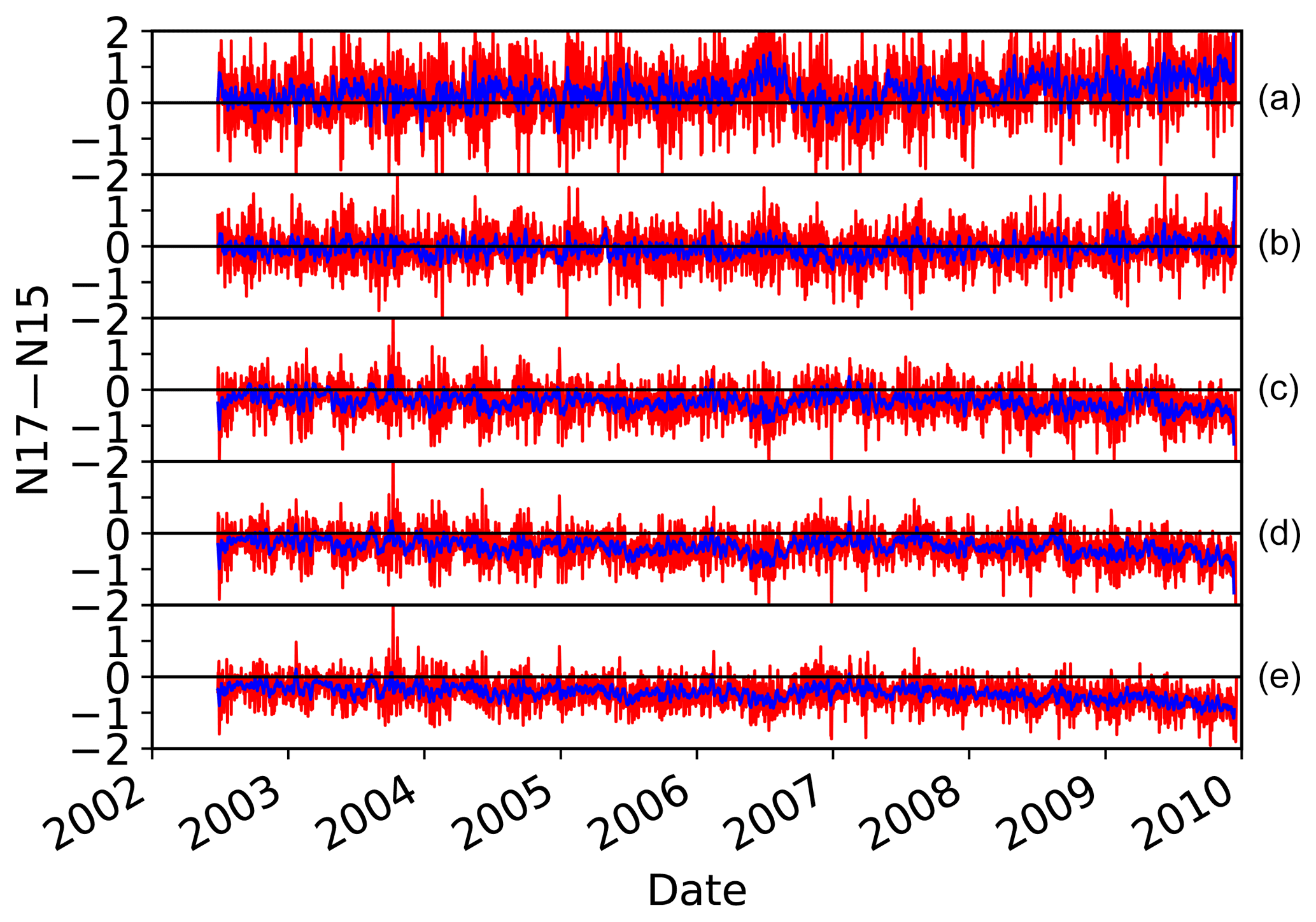
Figure 1Differences between all-sky N15 minus N17 and clear-sky N15 minus N17 (channels 1–5 from a to e). The values are differences between all-sky NOAA-15 and NOAA-17 measurements minus the differences between the two satellites in clear-sky conditions. The blue lines show the weekly-moving averages.
4.2 Diurnal cycle effect
The effect of land and ocean on the intercalibration, which is due to a stronger diurnal cycle over land, especially for the near surface-peaking channels, was investigated by separating land and ocean brightness temperatures over the tropical region, then calculating the intercalibration coefficients. Similarly to the impact of clouds, we employed double differences to evaluate the impact of a larger diurnal cycle over land on the inter-satellite differences. In this case, the double difference is calculated as the difference of the differences between land and ocean brightness temperatures of AMSU-B on board NOAA-15 vs. NOAA-17. If we indicate reference (NOAA-17) and target (NOAA-15) instruments using r and t indices and land and ocean using L and O, then the double difference is calculated as . Figure 2 shows an example of double differences between collocated brightness temperatures of NOAA-17 (reference satellite) and NOAA-15 (target satellite) over land and ocean. As expected, the surface channels are more sensitive to the diurnal cycle of Tb over land and a small trend after 2005 is observed that can be explained by the orbital drift of both satellites. The double difference is maximum around 2005 when the NOAA-15 ascending (descending) overpass was around 18:00 LT (06:00 LT) and NOAA-17 ascending (descending) overpass time was around 22:30 LT (10:30 LT). Therefore, the intercalibration was limited to tropical oceans to avoid the effect of a diurnal cycle. Since during polar winters, that region is normally covered by ice and snow, we averaged all the data over polar regions and no land–ocean mask was applied. All the experiments for this section were conducted using clear-sky data.

Figure 2Difference between N17 minus N15 over land and N17 minus N15 over ocean in the tropical region. The blue lines show the weekly-moving averages. (a)–(e) are channels 1–5.
4.3 Polarization difference
Although AMSU-B and MHS are two similar instruments, there are several differences in terms of polarization and frequency of some of their channels. Both instruments have single polarization at nadir. All AMSU-B channels and channels 1, 2 and 5 of MHS are vertically polarized but channels 3 and 4 of MHS are horizontally polarized at nadir (Kidwell et al., 2009). The vertical and horizontal components of the polarized radiation are the same over ocean at the nadir location, but the polarization changes as the antenna moves toward the edge of the swath. Therefore, the inter-satellite differences at nadir should not significantly depend on the channels' polarization, but as the antenna rotates the polarization becomes mixed and introduces differences. Other factors that may impact off-nadir differences include the scan-angle dependent bias as well as change in the height of the weighting functions.
Figure 3 shows the inter-satellite differences for NOAA-17 AMSU-B and NOAA-18 MHS vs. FOVs averaged over tropical oceans for the entire period. The FOV numbers start from the left side of the scan (FOV1), so that the nadir view is FOV45 and the most right view is FOV90. Note that the NOAA-18 overpass time is around 13:00 LT but the NOAA-17 overpass time is around 22:00 LT. As shown in Fig. 3, the differences between the two instruments significantly change with FOV, especially for Channel 1. Figure 4 shows the time series of the differences between the two instruments. As shown in Fig. 4, the differences exist for the entire period, and other than some small variations, do not vary with time. Figure 5 shows the difference between the two instruments over tropical land. If the differences were due to different overpass times, then the differences between the two instruments should be larger over land. However, not only are the differences generally smaller over land but also they do not depend on the FOV. Since the ocean is a polarizer in MW frequencies but the land generally is not a polarizer, the difference between Figs. 4 and 5 particularly highlights the effect of polarization on the differences between the two instruments over tropical oceans. Note that this exercise is not able to rule out other factors that may affect the inter-satellite differences. One possible explanation is that the weighting functions peak higher as the field of view moves from nadir to the edge of the scan so that some of the FOVs peak high enough in the atmosphere to become insensitive to the surface conditions.

Figure 3Effect of polarization on the difference between NOAA-17 AMSU-B and NOAA-18 MHS observations averaged over tropical ocean for different FOVs.
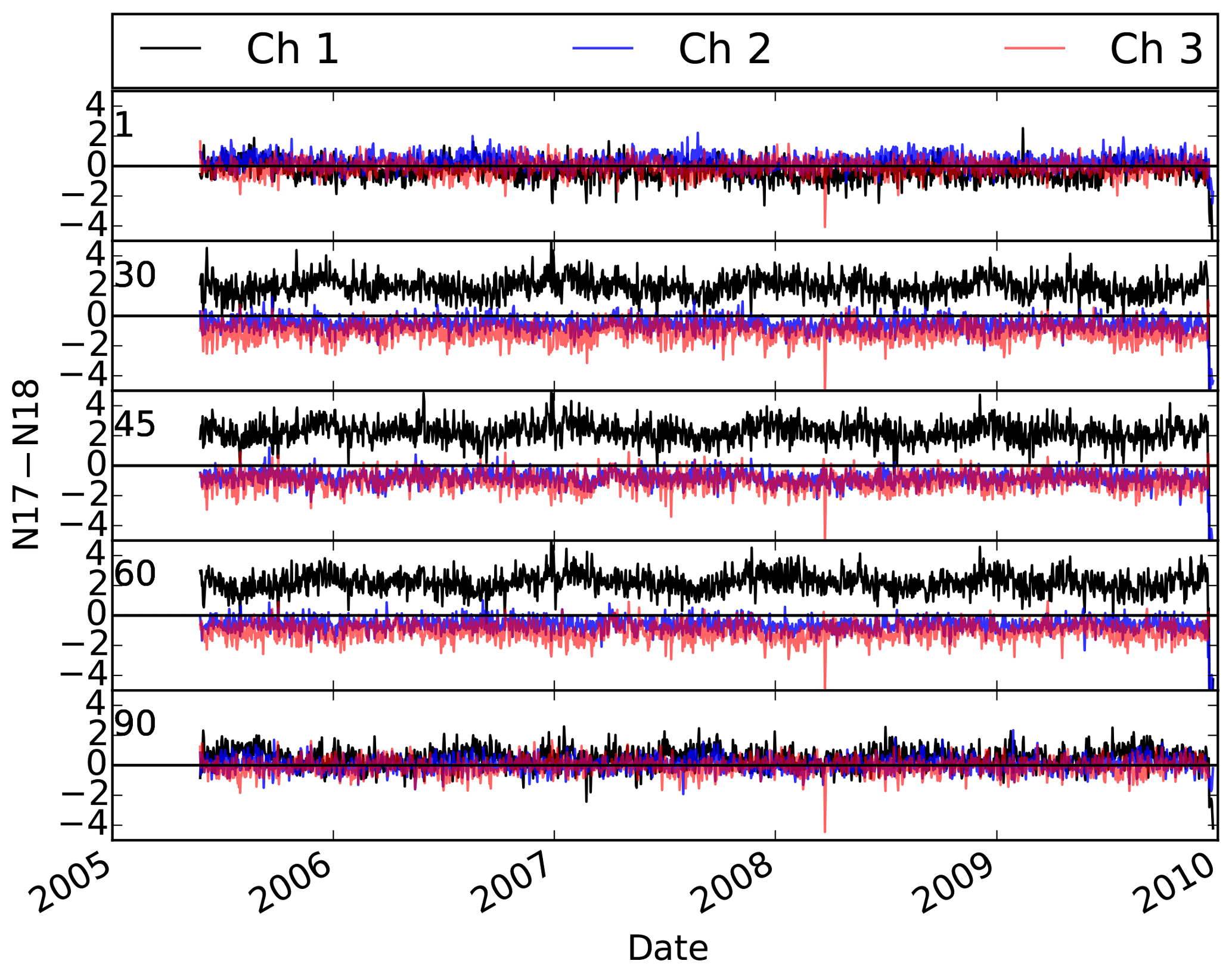
Figure 4Effect of polarization on the difference between NOAA-17 AMSU-B and NOAA-18 MHS observations for different FOVs over tropical ocean. FOV numbers are printed on the left side of each subplot. Channels 4 and 5 are not included because they were very similar to Channel 3.
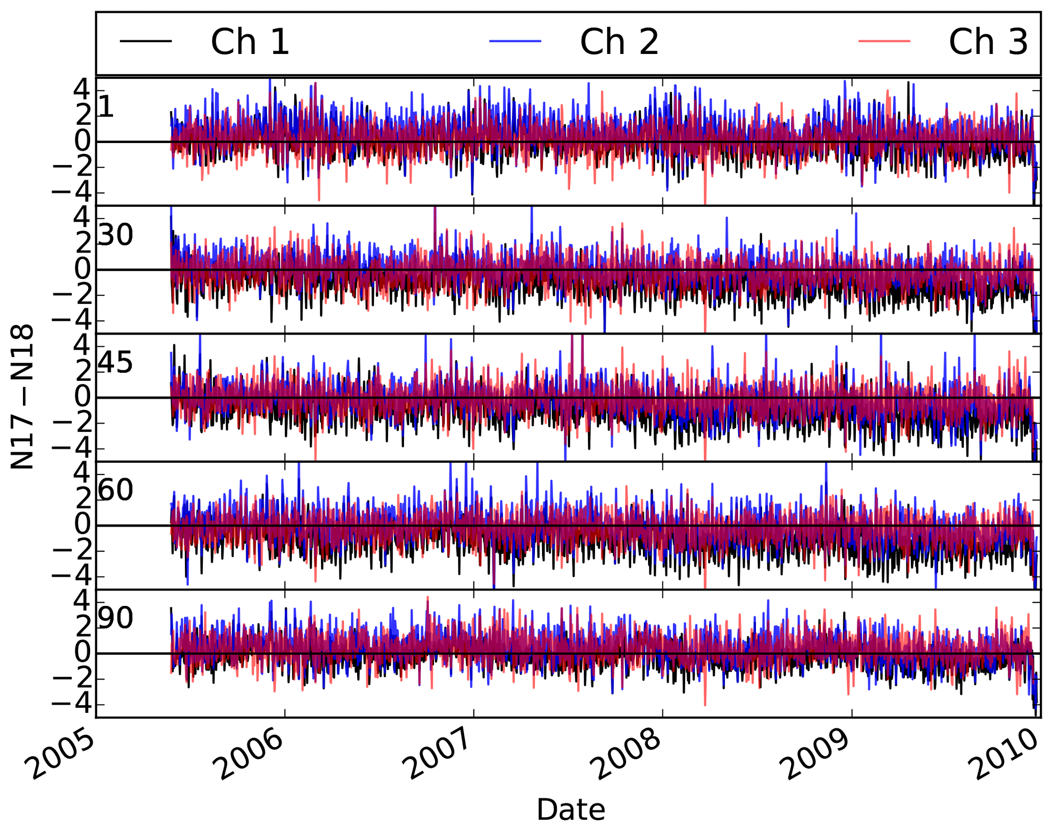
Figure 5Effect of polarization on the difference between NOAA-17 AMSU-B and NOAA-18 MHS observations for different FOVs over tropical land. FOV numbers are printed on the left side of each subplot.
4.4 Reference instrument
As stated before, due to the lack of reference measurements, one of the instruments which is stable over time is chosen as the reference instrument and the other instruments (target instruments) are calibrated with respect to it. Determining the reference instrument is likely to be the biggest challenge in conducting intercalibration. All other instruments will be corrected with respect to the reference instrument; therefore selecting a biased instrument as the reference instrument means that the intercalibrated measurements will suffer from an even larger bias than the original measurements. Because of the lack of reference measurements, it is almost impossible to select an instrument as a reference without any uncertainty. One important feature of the intercalibrated measurements is that they are expected to be representative of the climate; thus they may be used for studies related to climate change and variability. As stated before, because of negligible diurnal cycle over the tropical oceans, the orbital drift should not introduce a significant trend in the observations. Thus variability in the measurements averaged over the tropical oceans is expected to be similar to that reported for geophysical variables affecting the brightness temperatures. For instance, variability in the measurements of surface sensitive channels is expected to be very close to the change in surface temperature as the brightness temperatures for those channels are mostly affected by the surface temperature and emissivity. Since the emissivity is not expected to change with time, the variability in the brightness temperatures is expected to follow the change in surface temperature. Figure 6 shows the averages over tropical oceans for different satellites and all five AMSU-B/MHS channels. As mentioned before, we decided not to intercalibrate AMSU-B with MHS measurements; therefore we were required to select one satellite as the reference for the AMSU-B instruments and one for the MHS instruments. NOAA-16 channels 3–5 show a large drift with time; therefore NOAA-16 was excluded. NOAA-15 experienced some calibration issues, especially with regard to RFI; thus we decided to use NOAA-17 AMSU-B as the reference instrument for the AMSU-B instruments. There is a good consistency between NOAA-17 and NOAA-15 Channel 1, but a systematic difference between AMSU-B and MHS observations for Channel 1. Additionally, there is a systematic difference between NOAA-17 Channel 4 and MHS observations for the same channel. Although NOAA-15 matches MHS data during that time frame, that is basically caused by a positive and then a reverse trend in the NOAA-15 observations. The MHS instruments are generally consistent with each other, but we choose NOAA-18 for the reference satellite because the data are available for a longer time period.
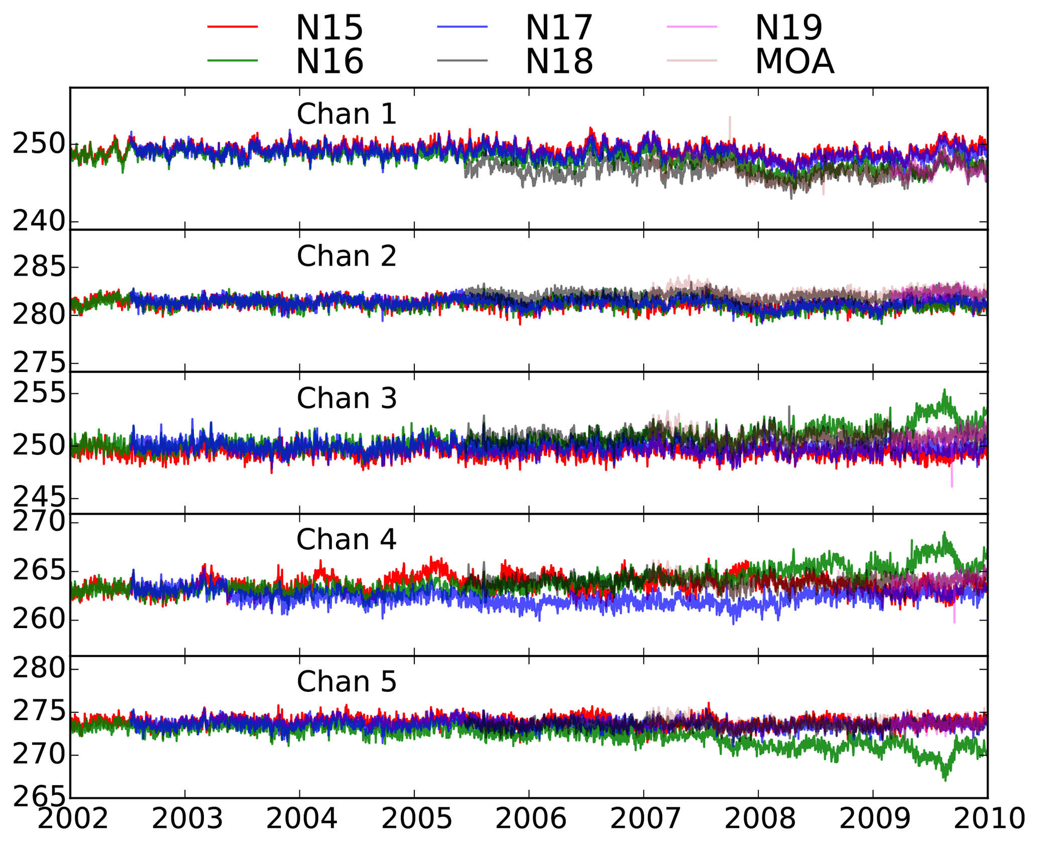
Figure 6Analysis of the time series of observations averaged over the tropical oceans for selecting the reference satellites. NOAA-19 and MetOp-A (MOA) are intercalibrated with reference to MHS on board NOAA-18.
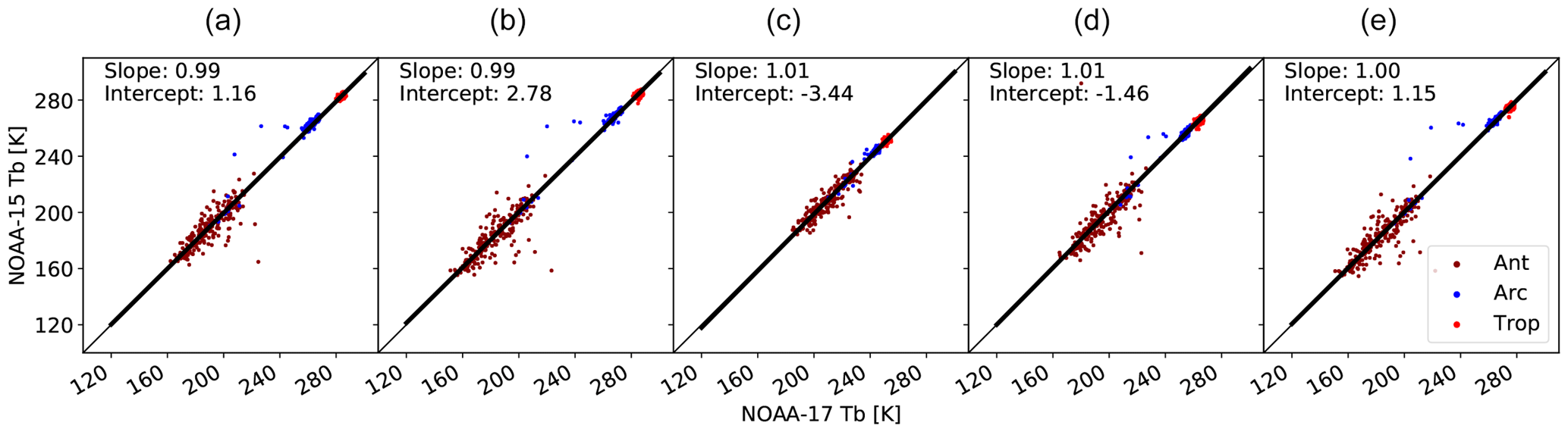
Figure 7Determining the empirical calibration coefficients using a linear relation between the measurements from the target and reference instruments. (a)–(e) are channels 1–5 from left to right. The solid black line shows the regression line. Different colors show the data for Antarctic (Ant), Arctic (Arc), and tropical (Trop) regions.
4.5 Intercalibration coefficients
The primary measurement of the microwave instruments is digital counts which are converted through a two-point calibration into radiances or brightness temperatures. The calibration equation is based on the relation between digital counts and measured radiances for a radiometrically cold reference (normally when the instrument measures the background space radiance) and a hot (warm) reference (normally a blackbody on board the satellite). The radiometric error can change with scene temperature if the error is not stable from one load to the other one due to, for instance, non-linearity in the calibration. Because of this scene dependency, it is required to evaluate the inter-satellite differences for a wide range of brightness temperatures. This is one of the main reasons that SNOs are not sufficient for the intercalibration of microwave instruments, as SNOs normally occur at high latitudes and only cover a small range of Tbs. In this study, we utilized the averages of brightness temperatures over the tropical region at one end of the measurements and the polar averages at the other end. Note that either of these can form the lowest or highest values depending on the channel as well as the surface type. As stated earlier, we only used the brightness temperatures over ocean to calculate the tropical averages.
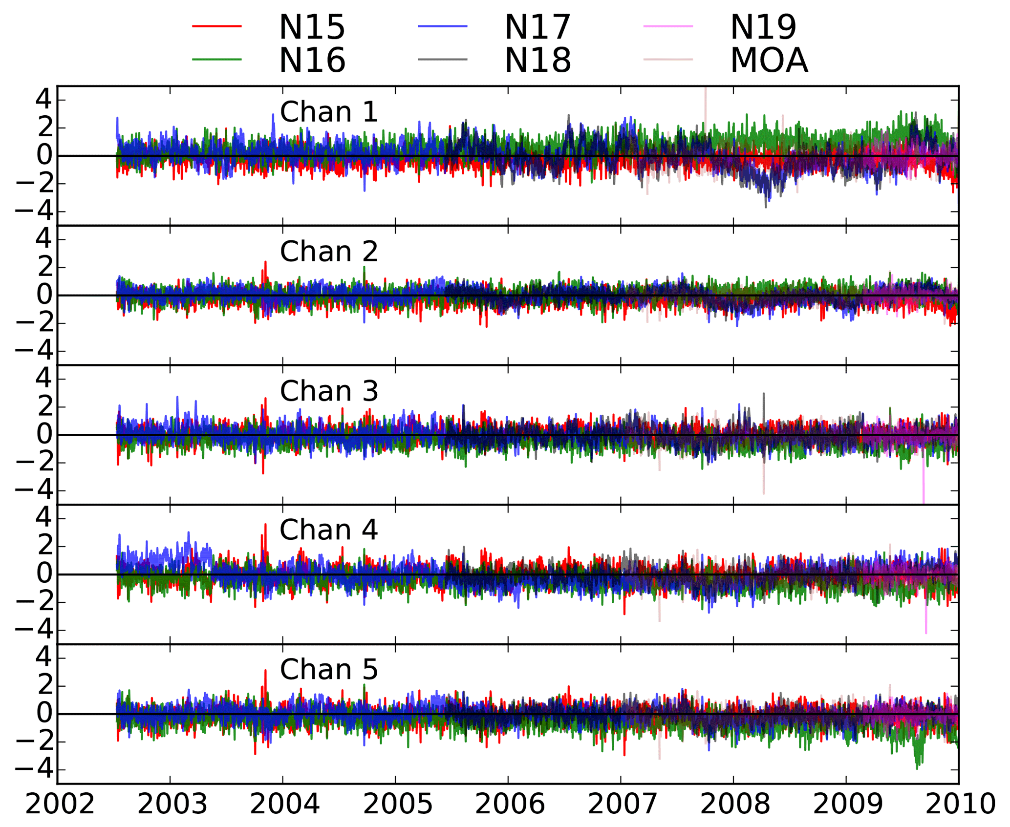
Figure 9Intercalibrated time series of AMSU-B and MHS observations. NOAA-19 and MetOp-A (MOA) are intercalibrated with reference to MHS on board NOAA-18.
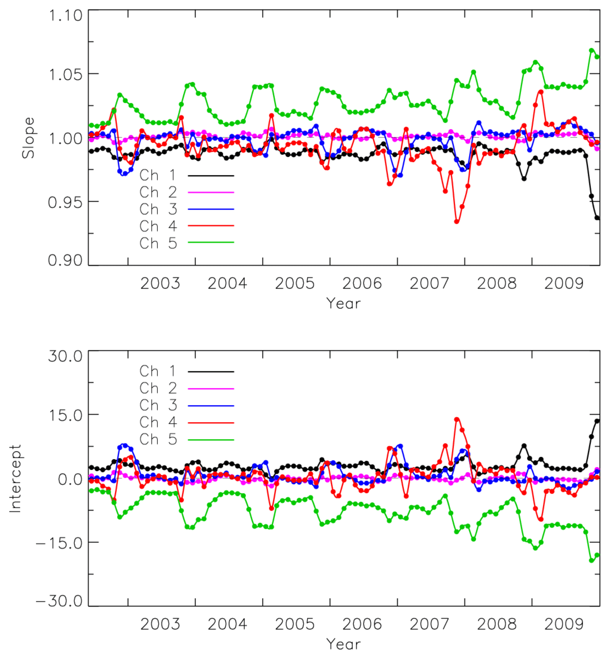
Figure 7 shows an example of the relation between Tbs from reference and target instruments. All the coefficients are derived using a linear relation as we did not have any evidence of the non-linearity between the differences in target and reference instruments. The calibration coefficients were calculated as , where Tbt and Tbr refer to the measurements from the target and reference instruments. The intercalibration coefficients were calculated on a monthly basis, then were interpolated to daily values using cubic-spline functions. This helps to reduce the noise in the coefficients. Therefore, the intercalibration process can be explained as follows: (1) data are averaged over the clear-sky tropical oceans and polar nights, (2) 1 month of data from both regions are used to make the scatterplots between reference and target satellites, (3) monthly intercalibration coefficients are calculated, then interpolated to daily values, (4) the coefficients are applied to level-1b data to calculate the intercalibrated brightness temperatures.
We did not find any advantage to use moving-window averages, i.e., collocate 1 month of data around the day of interest, then move the window to other days. Figure 8 shows an example of the monthly intercalibration coefficients as well as interpolated values. We also found that calculating the intercalibration coefficients on an annual basis is not enough since there might be short-term changes in the data that cannot be accounted for using annual coefficients. NOAA-15 was launched in 1998 but NOAA-17 data are only available since 2002. Since extrapolation of the coefficients is not recommended, we intercalibrated NOAA-15 data before 2002 using the coefficients calculated based on NOAA-15 and NOAA-17 2002 data. The only problem with this method is that the pre-2002 trend in NOAA-15 data is removed.
The results were evaluated using area-averaged values over the tropical oceans. Figure 9 shows the time series of intercalibrated brightness temperatures. The time series for NOAA-17 and NOAA-18 are only subtracted from their own mean values for the entire period. Overall, the intercalibrated Tbs are consistent with each other within about 0.5 K. However, there are some periods where the differences are even larger than 1.0 K. The difference between intercalibrated NOAA-15 and NOAA-17 observations is generally less than that for NOAA-16 and NOAA-17. For instance, around 2009, NOAA-16 Channel 5 observations show a difference of up to 2.0 K compared to NOAA-17 Channel 5 measurements. Given that the goal of study was not to completely remove the differences between measurements from different instruments but rather to remove possible biases in the measurements, the consistency observed in Fig. 9 is very satisfactory. In the 183 GHz frequencies, a 1 degree kelvin change in brightness temperature is roughly equal to a 7 %–10 % change in relative humidity (Moradi et al., 2015b); therefore it is expected that the derived humidity products have an error less than 10 %.
Satellite observations from AMSU-B and MHS are used to retrieve global climate and hydrological products such as water vapor, precipitation, and ice cloud parameters. However, these observations are prone to errors and uncertainties that can be classified into radiometric and geometric errors. In the current study, we quantified and corrected the radiometric errors in these observations for the period of 2000–2010. The AMSU-B observations suffer from several instrument failure after 2010. Work is currently under progress to correct some of the AMSU-B observations for the period 2010–2015. A unique characteristic of the radiometric error is that it changes with the scene temperature. A common technique that is used for the radiometric correction is intercalibration of observations measured by similar instruments. A key parameter in intercalibrating satellite observations is to find coincident observations or observations for the same location and same time. Since finding such coincident observations is challenging, we used daily averages of brightness temperatures over regions with negligible diurnal variations. In this study, we used monthly averages of measurements over the tropical oceans and nighttime polar regions to perform the intercalibration. In this two-point scheme, the intercalibration coefficients are calculated using monthly averages, then interpolated to the daily values using a cubic spline. We selected AMSU-B on board NOAA-17 as the reference instrument for all AMSU-B instruments and MHS on board NOAA-18 as the reference for all MHS instruments. We did not intercalibrate AMSU-B and MHS because of some differences in the frequency and polarization among the two instruments. Most AMSU-B channels on board NOAA-16 and channels 1 and 4 of AMSU-B on board NOAA-15 showed a large drift with time and were corrected with respect to NOAA-17 data. Measurements from MHS instruments were very consistent. Selecting a reference instrument is the most challenging part of the intercalibration because of the lack of reference observations. Selecting a biased reference instrument means that all the intercalibrated measurements will be biased. Another challenge is the intercalibration of cloud-contaminated observations. Due to a larger diurnal variation for the clouds over the tropical regions, we only used clear-sky observations to perform the intercalibrations. Neither the simultaneous nadir observations nor the technique used in this study can be used for the intercalibration of cloud-contaminated measurements because of the dynamic nature of the clouds.
The satellite observations used in the study are available free of charge from the NOAA Comprehensive Large Array-data Stewardship System (CLASS) at https://www.class.noaa.gov/ (last access: 1 September 2018). The reprocessed observations are available from the NOAA Climate Data Record Program (Ferraro et al., 2018).
The authors declare that they have no conflict of interest.
This study was supported by NOAA grant no. NA09NES4400006 (Cooperative
Institute for Climate and Satellites – CICS) at the University of Maryland,
Earth System Science Interdisciplinary Center (ESSIC). The views, opinions,
and findings contained in this report are those of the authors and should not
be construed as an official National Oceanic and Atmospheric Administration
or U.S. Government position, policy, or decision.
Edited by: Murray Hamilton
Reviewed by: two anonymous referees
Berg, W., Bilanow, S., Chen, R., Datta, S., Draper, D., Ebrahimi, H., Farrar, S., Jones, W. L., Kroodsma, R., McKague, D., Payne, V., Wang, J., Wilheit, T., and Yang, J. X.: Intercalibration of the GPM Microwave Radiometer Constellation, J. Atmos. Ocean. Tech., 33, 2639–2654, https://doi.org/10.1175/JTECH-D-16-0100.1, 2016. a
Buehler, S. A., Kuvatov, M., Sreerekha, T. R., John, V. O., Rydberg, B., Eriksson, P., and Notholt, J.: A cloud filtering method for microwave upper tropospheric humidity measurements, Atmos. Chem. Phys., 7, 5531–5542, https://doi.org/10.5194/acp-7-5531-2007, 2007. a
Cao, C., Weinreb, M., and Xu, H.: Predicting Simultaneous Nadir Overpasses among Polar-Orbiting Meteorological Satellites for the Intersatellite Calibration of Radiometers, J. Atmos. Ocean. Techn., 21, 537–542, https://doi.org/10.1175/1520-0426(2004)021<0537:PSNOAP>2.0.CO;2, 2004. a
Chander, G., Hewison, T., Fox, N., Wu, X., Xiong, X., and Blackwell, W.: Overview of intercalibration of satellite instruments, IEEE T. Geosci. Remote, 51, 1056–1080, https://doi.org/10.1109/TGRS.2012.2228654, 2013. a
Ferraro, R., Weng, F., C. Grody, N., Zhao, L., Meng, H., Kongoli, C., Pellegrino, P., Qiu, S., and Dean, C.: NOAA operational hydrological products derived from the AMSU, IEEE T. Geosci. Remote, 43, 1036–1049, 2005. a
Ferraro, R. R., Meng, H., and NOAA CDR Program: NOAA Climate Data Records (CDR) of AMSU-A/B and MHS Hydrological Properties, Version 1, NOAA National Centers for Environmental Information, https://doi.org/10.7289/V5V69GM6, 2018. a
Hewison, T. and Saunders, R.: Measurements of the AMSU-B antenna pattern, IEEE T. Geosci. Remote, 34, 405–412, https://doi.org/10.1109/36.485118, 1996. a, b, c
John, V. O., Holl, G., Buehler, S. A., Candy, B., Saunders, R. W., and Parker, D. E.: Understanding intersatellite biases of microwave humidity sounders using global simultaneous nadir overpasses, J. Geophys. Res., 117, 13, D02305, https://doi.org/10.1029/2011JD016349, 2012. a, b
Kerola, D. X.: Calibration of Special Sensor Microwave Imager/Sounder (SSMIS) upper air brightness temperature measurements using a comprehensive radiative transfer model, Radio Sci., 41, RS4001, https://doi.org/10.1029/2005RS003329, 2006. a
Kidwell, K. B., Goodrum, G., and Winston, W.: NOAA KLM user's guide, with NOAA-N, -N' supplement, Tech. rep., National Environmental Satellite, Data, and Information Services, Silver Spring, MD, 2009. a, b, c
Mo, T.: Postlaunch Calibration of the NOAA-18 Advanced Microwave Sounding Unit-A, IEEE T. Geosci. Remote, 45, 1928–1937, https://doi.org/10.1109/TGRS.2007.897451, 2007. a
Moradi, I., Meng, H., Ferraro, R., and Bilanow, S.: Correcting Geolocation Errors for Microwave Instruments Aboard NOAA Satellites, IEEE T. Geosci. Remote, 51, 3625–3637, https://doi.org/10.1109/TGRS.2012.2225840, 2013a. a, b, c
Moradi, I., Soden, B., Ferraro, R., Arkin, P., and Vömel, H.: Assessing the quality of humidity measurements from global operational radiosonde sensors, J. Geophys. Res.-Atmos., 118, 8040–8053, https://doi.org/10.1002/jgrd.50589, 2013b. a
Moradi, I., Ferraro, R., Eriksson, P., and Weng, F.: Intercalibration and Validation of Observations From ATMS and SAPHIR Microwave Sounders, IEEE T. Geosci. Remote, 53, 5915–5925, https://doi.org/10.1109/TGRS.2015.2427165, 2015a. a, b, c
Moradi, I., Ferraro, R., Soden, B., Eriksson, P., and Arkin, P.: Retrieving Layer-Averaged Tropospheric Humidity From Advanced Technology Microwave Sounder Water Vapor Channels, IEEE T. Geosci. Remote, 53, 6675–6688, https://doi.org/10.1109/TGRS.2015.2445832, 2015b. a, b
Moradi, I., Arkin, P., Ferraro, R., Eriksson, P., and Fetzer, E.: Diurnal variation of tropospheric relative humidity in tropical regions, Atmos. Chem. Phys., 16, 6913–6929, https://doi.org/10.5194/acp-16-6913-2016, 2016. a
Przybylak, R.: Diurnal temperature range in the Arctic and its relation to hemispheric and Arctic circulation patterns, Int. J. Climatol., 20, 231–253, https://doi.org/10.1002/(SICI)1097-0088(20000315)20:3<231::AID-JOC468>3.0.CO;2-U, 2000. a, b
Przybylak, R.: The climate of the Arctic, vol. 52, Springer, the Netherlands, https://doi.org/10.1007/978-94-017-0379-6, 2016. a, b
Rienecker, M. M., Suarez, M. J., Gelaro, R., Todling, R., Bacmeister, J., Liu, E., Bosilovich, M. G., Schubert, S. D., Takacs, L., Kim, G.-K., Bloom, S., Chen, J., Collins, D., Conaty, A., da Silva, A., Gu, W., Joiner, J., Koster, R. D., Lucchesi, R., Molod, A., Owens, T., Pawson, S., Pegion, P., Redder, C. R., Reichle, R., Robertson, F. R., Ruddick, A. G., Sienkiewicz, M., and Woollen, J.: MERRA: NASA's Modern-Era Retrospective Analysis for Research and Applications, J. Climate, 24, 3624–3648, https://doi.org/10.1175/JCLI-D-11-00015.1, 2011. a
Ruf, C.: Detection of calibration drifts in spaceborne microwave radiometers using a vicarious cold reference, IEEE T. Geosci. Remote, 38, 44–52, https://doi.org/10.1109/36.823900, 2000. a
Sapiano, M., Berg, W., McKague, D., and Kummerow, C.: Toward an Intercalibrated Fundamental Climate Data Record of the SSM/I Sensors, IEEE T. Geosci. Remote, 51, 1492–1503, https://doi.org/10.1109/TGRS.2012.2206601, 2013. a, b
Saunders, R., Blackmore, T., Candy, B., Francis, P., and Hewison, T.: Monitoring Satellite Radiance Biases Using NWP Models, IEEE T. Geosci. Remote, 51, 1124–1138, https://doi.org/10.1109/TGRS.2012.2229283, 2013. a, b
Shi, L. and Bates, J. J.: Three decades of intersatellite-calibrated High-Resolution Infrared Radiation Sounder upper tropospheric water vapor, J. Geophys. Res.-Atmos., 116, D04108, https://doi.org/10.1029/2010JD014847, 2011. a, b
Wessel, J., Farley, R. W., Fote, A., Hong, Y., Poe, G. A., Swadley, S. D., Thomas, B., and Boucher, D. J.: Calibration and Validation of DMSP SSMIS Lower Atmospheric Sounding Channels, IEEE T. Geosci. Remote, 46, 946–961, https://doi.org/10.1109/TGRS.2008.917132, 2008. a
Wilheit, T.: Comparing Calibrations of Similar Conically Scanning Window-Channel Microwave Radiometers, IEEE T. Geosci. Remote, 51, 1453–1464, https://doi.org/10.1109/TGRS.2012.2207122, 00006, 2013. a, b
Zou, C.-Z. and Wang, W.: Intersatellite calibration of AMSU-A observations for weather and climate applications, J. Geophys. Res., 116, D23113, https://doi.org/10.1029/2011JD016205, 2011. a