the Creative Commons Attribution 4.0 License.
the Creative Commons Attribution 4.0 License.
 | 18 Dec 2018
A physics-based approach to oversample multi-satellite, multispecies observations to a common grid
Karen Cady-Pereira
Christopher Chan Miller
Kelly Chance
Lieven Clarisse
Pierre-François Coheur
Gonzalo González Abad
Guanyu Huang
Xiong Liu
Martin Van Damme
Mark Zondlo
Satellite remote sensing of the Earth's atmospheric composition usually samples irregularly in space and time, and many applications require spatially and temporally averaging the satellite observations (level 2) to a regular grid (level 3). When averaging level 2 data over a long period to a target level 3 grid that is significantly finer than the sizes of level 2 pixels, this process is referred to as “oversampling”. An agile, physics-based oversampling approach is developed to represent each satellite observation as a sensitivity distribution on the ground, instead of a point or a polygon as assumed in previous methods. This sensitivity distribution can be determined by the spatial response function of each satellite sensor. A generalized 2-D super Gaussian function is proposed to characterize the spatial response functions of both imaging grating spectrometers (e.g., OMI, OMPS, and TROPOMI) and scanning Fourier transform spectrometers (e.g., GOSAT, IASI, and CrIS). Synthetic OMI and IASI observations were generated to compare the errors due to simplifying satellite fields of view (FOVs) as polygons (tessellation error) and the errors due to discretizing the smooth spatial response function on a finite grid (discretization error). The balance between these two error sources depends on the target grid size, the ground size of the FOV, and the smoothness of spatial response functions. Explicit consideration of the spatial response function is favorable for fine-grid oversampling and smoother spatial response. For OMI, it is beneficial to oversample using the spatial response functions for grids finer than ∼16 km. The generalized 2-D super Gaussian function also enables smoothing of the level 3 results by decreasing the shape-determining exponents, which is useful for a high noise level or sparse satellite datasets. This physical oversampling approach is especially advantageous during smaller temporal windows and shows substantially improved visualization of trace gas distribution and local gradients when applied to OMI NO2 products and IASI NH3 products. There is no appreciable difference in the computational time when using the physical oversampling versus other oversampling methods.
- Article
(6093 KB) - Full-text XML
- BibTeX
- EndNote


Since the launch of the ESA Global Ozone Monitoring Experiment (GOME) in 1995, satellite observations have tremendously advanced our understanding of the processes governing the atmospheric composition, greenhouse gas emissions, and air quality (Jacob et al., 2016; Martin, 2008; Streets et al., 2013). Global distributions of atmospheric species that play critical roles in atmospheric chemistry and air pollution, such as ozone (Bak et al., 2017), NO2 (Krotkov et al., 2017), SO2 (Li et al., 2017a), formaldehyde (González Abad et al., 2015), glyoxal (Chan Miller et al., 2014), and BrO (Suleiman et al., 2018), have been retrieved from the backscattered solar UV–visible spectra observed by generations of polar-orbiting satellite sensors, including GOME (Burrows et al., 1999), SCIAMACHY (Bovensmann et al., 1999), OMI (Levelt et al., 2018), GOME-2 (Munro et al., 2016), OMPS (Rodriguez et al., 2003), and TROPOMI (Veefkind et al., 2012). A constellation of geostationary satellites will provide hourly measurements of these species over North America, Europe, and Asia in the near future (Zoogman et al., 2017). Observations of the backscattered shortwave infrared solar spectra also enable the retrieval of CO2, CH4, and/or CO from SCIAMACHY (Buchwitz et al., 2005), GOSAT (Yoshida et al., 2011), OCO-2 (Eldering et al., 2017), and TROPOMI (Borsdorff et al., 2018; Hu et al., 2018). Moreover, many atmospheric species have strong spectroscopic signatures in the mid-infrared and can be retrieved from the Earth's thermal emission spectra collected by satellite sensors such as MOPITT (Drummond et al., 2010), AIRS (Aumann et al., 2003), TES (Bowman et al., 2006), IASI (Clerbaux et al., 2009), and CrIS (Han et al., 2013). One species of particular significance to tropospheric chemistry and air quality is NH3 (Baek et al., 2004; Paulot and Jacob, 2014), which has been successfully retrieved from TES (Shephard et al., 2011; Sun et al., 2015a), AIRS (Warner et al., 2016), IASI (Clarisse et al., 2010; Van Damme et al., 2017; Whitburn et al., 2016a), and CrIS (Dammers et al., 2017; Shephard and Cady-Pereira, 2015).
The retrieval results from satellite sensors are usually total or partial (e.g., tropospheric or planetary boundary layer, PBL) column density at individual satellite pixels, i.e., the level 2 product. However, the pixel geometry may vary significantly even for the same sensor (see Fig. 1 for example), and data quality screening (by cloud coverage, solar zenith angle, surface albedo, thermal contrast, etc.) often leaves only small and patchy fractions of useful level 2 pixels for any given orbit. As such, the level 2 data over many orbits are often projected to a regular spatial grid to better represent the spatiotemporal variations of the target species through a gridding algorithm. These “level 3” products help to average out the observational noise that can be significant for individual level 2 retrieval and make satellite data more accessible for scientific studies and the general public. These products may also lead to additional discoveries, such as emission and lifetime estimates (Beirle et al., 2011; Fioletov et al., 2017, 2015; Liu et al., 2016; Valin et al., 2013; Whitburn et al., 2015, 2016b; Zhu et al., 2014; de Foy et al., 2015), source identification (Kort et al., 2014; McLinden et al., 2012, 2016), trend analyses (Duncan et al., 2016; Lamsal et al., 2015; Russell et al., 2012; Warner et al., 2017; Zhu et al., 2017b), assessment of environmental exposure for public health (Geddes et al., 2016; Zhu et al., 2017a), and satellite data validation (Zhu et al., 2016).
The operational level 3 products are typically provided at grid sizes of or even , which are too coarse for regional heterogeneous emission sources (e.g., urban areas), especially for species with short lifetimes. These level 3 products are provided at fixed temporal intervals (e.g., daily, monthly, and annually). To customize the temporal and spatial sampling intervals, one often needs to regrid the level 2 data.
Various gridding algorithms have been developed to generate level 3 maps at a regional scale with much finer grids (0.05–0.01∘) than the sizes of level 2 pixels, and this process is generally referred to as “oversampling” (Russell et al., 2010; de Foy et al., 2009). In this work, we present an agile, physics-based oversampling approach that represents each level 2 satellite pixel as a sensitivity distribution on the Earth's surface (e.g., the spatial response function), instead of a point or a polygon as assumed in previous methods. A generalized 2-D super Gaussian function is used to characterize the spatial response functions of both imaging grating spectrometers (e.g., OMI, OMPS, and TROPOMI) and scanning Fourier transform spectrometers (FTSs; e.g., GOSAT, IASI and CrIS). Applications to multiple existing satellite datasets are also highlighted.
2.1 OMI
The OMI instrument aboard the Aura satellite launched in 2004 is a push-broom UV–visible imaging grating spectrometer. It has a daytime equatorial crossing at ∼13:42 LT (local time). During normal global observation mode, the backscattered sunlight from the Earth is imaged by a telescope onto a rectangular entrance slit perpendicular to the flight direction. The light coming through the slit, which corresponds to an across-track angle of 115∘, or 2600 km on the ground, is dispersed by optical gratings and mapped on two 2D CCD detectors. Each detector image is aggregated across-track (along the length of the slit) into 60 spectra, corresponding to 60 across-track spatial pixels for the UV2 (307–383 nm) and visible (349–504 nm) bands, as shown by Fig. 1. Although the spatial response functions of OMI pixels are nonuniform (Sihler et al., 2017; de Graaf et al., 2016), the OMI pixels are widely characterized as quadrilateral polygons defined by 75 % of the energy in the along-track field of view (FOV) and the halfway points of the across-track FOV (Kurosu and Celarier, 2010). These OMI pixel polygons are close to rectangles, ranging from 14 km×26 km at nadir (or 13 km×24 km if assuming nonoverlapping pixels) to 28 km×160 km at the swath edges. Alternatively, OMI pixels can be represented as tiled polygons with no overlap between adjacent pixels. These tiled pixels produce a seamless swath image but are less accurate, especially in the along-track direction. OMI is a highly successful mission with long data records, and most of the successor missions follow a similar design (Levelt et al., 2018). The oversampling technique demonstrated here can be readily adopted for a range of OMI products and OMI's successor missions, such as OMPS, TROPOMI, and TEMPO.

Figure 1Across-track (xtrack in figure) ground pixel geometry for IASI, CrIS, and the UV2 and VIS (visible) bands of OMI.
2.2 IASI
The IASI instrument is an FTS with an across-track scanning range of 2200 km (Fig. 1). It has a daytime equatorial crossing time of ∼09:30 LT. The first IASI instrument (IASI-A) was launched aboard the MetOp-A satellite in 2006, with the launch of IASI-B following in 2012 and IASI-C in 2018. IASI scans across the track with 30 mirror positions, or fields of regard (FORs), and each FOR is composed of a 2×2 array of pixels, or FOV. Each FOV projected on ground is a 12 km diameter circular footprint at nadir and elongates to ellipses towards the swath edges (Clerbaux et al., 2009). To simplify the ground pixel calculation, we represent each pixel as an ellipse with the major and minor axes and rotation angle interpolated from a lookup table based on latitude and FOR and FOV number.
We use the most recent neural network (NN) IASI NH3 retrieval based on calculation of a hyperspectral range index (HRI) and subsequent conversion to NH3 columns via a neural network (Van Damme et al., 2017; Whitburn et al., 2016a). The IASI NH3 datasets are publicly available for both IASI-A and IASI-B, with the version 2 (Van Damme et al., 2017) presenting significant improvements over version 1 (Whitburn et al., 2016a), including the negative values that are crucial for observational error averaging near the detection limit.
2.3 CrIS
The CrIS instrument, which is aboard the Suomi NPP satellite and the series of JPSS satellites, is a step-scan FTS with 2200 km across-track width (Fig. 1). It has a daytime equatorial crossing time of ∼13:30 LT. It has the same number of FORs as IASI, but each FOR contains 9 FOVs (3×3 array), providing a better spatial coverage. Each CrIS FOV is 14 km at nadir, slightly larger than IASI. Due to the mounting angle of the scanning mirror, the FOR rotates differently at each scanning angle. Similar to IASI, each CrIS pixel is represented as a rotated ellipse.
The CrIS fast physical retrieval (CFPR) NH3 retrieval product is based on the TES optimal estimation approach that minimizes the differences between spectral radiances and a simulated fast forward line-by-line model (Shephard and Cady-Pereira, 2015).
This section reviews existing gridding methods that map level 2 pixels to level 3 grids. Oversampling conventionally refers to the cases where level 3 grid is much finer than the level 2 pixel size.
3.1 Spatial interpolation
The spatial interpolation methods generate continuous data fields from observations made at discrete locations. The main difference between interpolation and the point- and polygon-based oversampling approaches discussed in Sect. 3.2 and 3.3 is that the values at grid cells that are not covered by satellite observations can be estimated. Therefore, the spatial interpolation methods are more commonly used for satellite datasets with significant spatial gaps or requiring additional smoothing. Common spatial interpolation methods include nearest neighbors, piecewise 2-D linear interpolation, spline interpolation, and various kriging methods. The moving window block kriging method has been proposed to generate global level 3 products for satellite observations of long-lived species, such as CH4 and CO2 (Tadić et al., 2015, 2017). A comprehensive review of available spatial interpolation methods for environmental variables is provided by Li and Heap (2014). There are relatively few applications of spatial interpolation methods to regional fine-grid oversampling, where each target grid cell usually receives a large number of overlapping satellite observations. Kuhlmann et al. (2014) proposed an interpolative gridding algorithm that reconstructs the trace gas distribution by a continuous parabolic spline surface, defined on the lattice of tiled satellite pixels. This approach produces smooth regional level 3 maps for the OMI NO2 products with specifically tuned smoothing parameters but has not been tested in non-tiled observations with significant numbers of missing values (e.g., IASI and CrIS).
3.2 Satellite observations as points
The simple “drop-in-the-box” gridding method can be classified into this category, as each satellite observation is assumed to be a point on the surface. The value for each target grid cell is the average of all screened satellite observations with the center of the FOV falling inside the grid cell boundaries. A conventional oversampling approach has been developed based on the drop-in-the-box method; instead of only averaging “in the box”, it includes satellite observations within a certain radius (much larger than the grid size) from the center of each grid cell. This averaging radius is chosen to balance the smoothing and noise but is also somewhat arbitrary. For example, McLinden et al. (2012) used a radius of 8 km to oversample the OMI NO2 tropospheric columns and a larger radius of 24 km to oversample the OMI SO2 total columns near the Canadian oil sands region; Fioletov et al. (2011) used 12 km to oversample the OMI SO2 total columns over the US; and Zhu et al. (2014) used 24 km to oversample the HCHO total columns near Houston, TX. This oversampling approach is referred to as “point oversampling” hereafter, as the pixel geometry is not considered. The pixel-specific observational errors are also not taken into account.
Figure 2 reconstructs a point oversampling process for an arbitrary target grid point (red star) located near Denver, CO. OMI NO2 data (Krotkov et al., 2017) over the year 2005 are used in this demonstration. Pixels with a cloud fraction ≥30 % or a solar zenith angle ≥75∘ are screened out. Only across-track positions with relatively small pixel areas (6–55 out of 1–60) are included, a common practice to oversample OMI data. Adding pixels at the swath edges would induce more “false negative” cases, as shown below. The screened satellite pixel centers that fall within a 12 km radius (dashed circle) are plotted as black points and red triangles. The red triangles are “false positive” observations because the corresponding pixel quadrilaterals, provided by the OMPIXCOR product, do not cover the target grid point. The pixel geometry of an extreme false positive case is illustrated by the pixel quadrilateral, featuring the largest separation between its boundary and the target grid point. Likewise, the false negative observations are plotted as purple squares, whose pixel centers fall outside the averaging circle (and hence not averaged), but these pixels cover the target grid point. An extreme case of the false negatives is also illustrated. For this example, there are 243 pixels within the 12 km radius, of which 54 are false positives (22 %). There are 92 false negatives (38 %) not included in the point oversampling. Typically, false positives are pixels closer to nadir, whereas false negatives are pixels away from nadir. In combination, the oversampled value at this grid location has contributions from a much different set of satellite observations than what should be represented. A larger averaging radius will decrease the occurrence of false negative cases but increase that of false positive cases. Because the OMI pixel dimension is larger at the across-track direction, these sampling biases differ in direction; observations in the across-track direction of the target grid point are more likely to become false negatives, and observations in the along-track direction are more likely to become false positives.
In reality, the OMI ground pixel footprints are not as sharp as quadrilateral boundaries (de Graaf et al., 2016), so the false positive and negative cases are not as well defined as in Fig. 2. This will be discussed in Sect. 4.1.
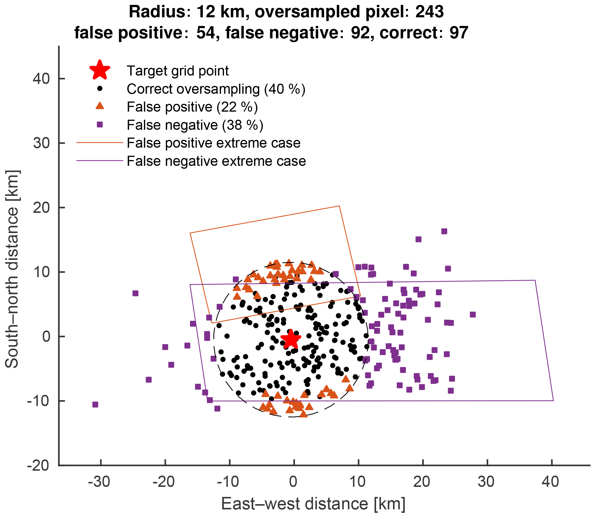
Figure 2Centers of screened OMI pixels in 2005 over a target grid point (red star) near Denver, CO. Pixels that overlap with the target grid point with the pixel center falling within the averaging radius (dashed circle) are plotted as black points (correct oversampling, 40 %). Pixels that overlap with the target grid point with the pixel center falling outside the averaging radius are plotted as purple squares (false negative, 38 %). Pixels that do not overlap with the target grid point with the pixel center falling in the averaging radius are plotted as red triangles (false positive, 22 %). Extreme cases of false positives or negatives are illustrated by OMI pixel quadrilaterals. The percentages of correct oversampling, false positive, and false negative pixels are labeled in the legend.
3.3 Satellite observations as polygons (i.e., tessellation)
This approach assumes that each satellite observation footprint is a polygon on the surface, and calculates the areal proportions of grid cells inside each polygon. Because calculating these overlapping areas requires filling irregular satellite footprint polygons with rectangular grid cells, it is also known as the “tessellation” approach. The contribution of each satellite observation to a given grid cell is weighted by the overlapping area and inversely weighted by the total pixel polygon area and the observational uncertainty, as shown by the following equations (Zhu et al., 2017a):
where
In the equations above, C(j) is the oversampled result for destination grid cell j; Ω(i) is the variable to be oversampled (e.g., total column) associated with the satellite pixel i; S(i,j) is the overlapping area between pixel i and grid cell j, and hence is the total area of pixel i, assuming that the grid extends beyond all pixel boundaries. When the destination grid is regular with constant grid cell area, it is convenient to normalize S(i,j) by the grid cell area, leading to overlapping fractions. We will follow this convention hereafter, and hence S(i,j) is always a dimensionless number. These equations take into account the extent of a pixel and give more weight to a nadir observation than to an observation at the edges of the satellite swath, where the information is more smeared out. The variable σ(i)p is the uncertainty term, and the power p has been assumed to be 1 (Zhu et al., 2017a) or 2 (Spurr, 2003; Van Damme et al., 2014) by different studies. If we assume each observation Ω(i) is a measurement of a constant true value with Gaussian random error σ(i), p=2 yields the maximum likelihood estimate of the true value. However, the true measurement and sampling errors often show heavier tails than a Gaussian distribution. In this study we adopt p=1, following Zhu et al. (2017a). The oversampled results are generally similar for both cases. Unlike the point oversampling discussed in Sect. 3.2 where C(j) is simply the average of Ω(i) within a circle, the tessellation approach fully utilizes the geometry and error information for each satellite observation. It has been adopted by many operational level 3 products and oversampling studies (Duncan et al., 2016; Kim et al., 2016; Krotkov, 2013; Li et al., 2017b; Liu et al., 2006; Van Damme et al., 2014; Wenig et al., 2008; Zhu et al., 2017a; de Foy et al., 2015).
It is sometimes convenient to define
to quantify the total number of overlapping pixel polygons used in averaging for grid cell j. Unlike the point oversampling, this number does not have to be an integer due to the consideration of partial overlaps. Because the location and size of these pixels vary day by day, averaging a large number of pixels reveals spatial patterns at scales finer than the satellite pixel scales, if these patterns are consistent through the averaging time period.
Figure 3 illustrates the tessellation process for OMI (a) and IASI (b) pixels, where the elliptical IASI pixel is represented by a 100-vertex polygon calculated from its minor/major axes and rotational angle lookup tables. The destination grid size is 5 km × 5 km, and the overlapping areas are normalized by the grid cell area (25 km2), as labeled in each grid cell.
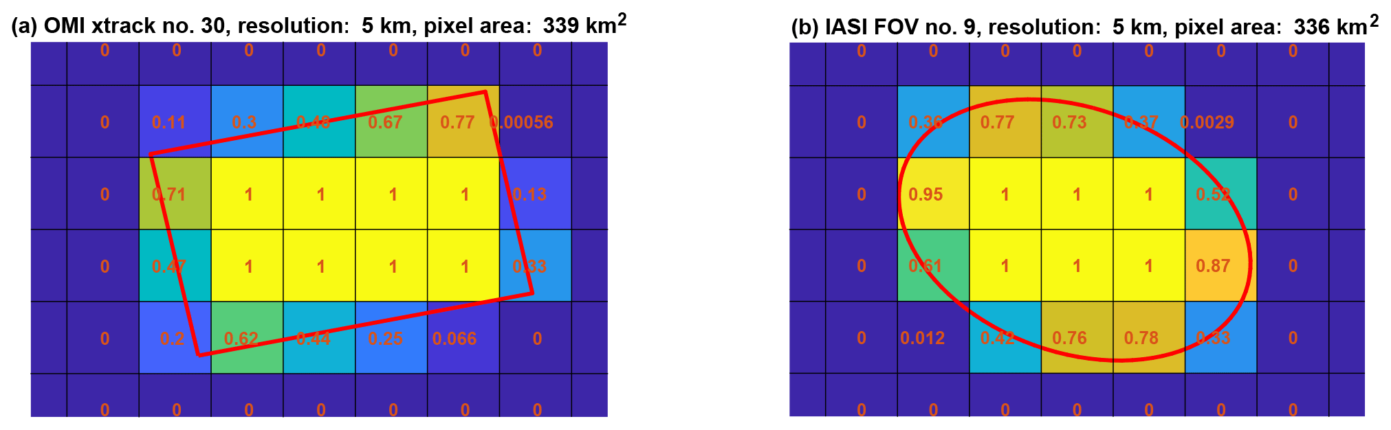
Figure 3Tessellation process for OMI (a) and IASI (b) pixels. The IASI pixel is approximated by a 100-vertex polygon. The overlapping area (S(i,j)) between satellite pixel i and grid cell j is labeled at grid cell center, normalized by grid cell area (25 km2). Across-track: xtrack.
4.1 Satellite observations as sensitivity distributions
The tessellation approach discussed in Sect. 3.3 inherently assumes that the satellite observation is uniformly sensitive to the scene inside the pixel polygon and has no sensitivity outside it. However, depending on target grid size and the spatial response function of specific satellite observations, this may be too strong of an assumption. For example, Schreier et al. (2010) characterized the complex spatial response function of the AIRS instrument and used it to improve the comparison of radiances measured by AIRS and MODIS. de Graaf et al. (2016) and Sihler et al. (2017) derived an in-flight spatial response function of OMI using collocated MODIS radiance. The operational Sentinel-5 Precursor, Sentinel-5, and Sentinel-4 cloud processors also rely on the spatial response functions of the imaging grating spectrometers to accurately calculate the cloud coverage within each FOV using collocated high-resolution cloud imagers (Siddans, 2017).
For imaging grating spectrometers like OMI, the spatial response function depends on the diffraction of the fore optics, the instantaneous field of view (i.e., the instantaneous projection of the slit on the ground from the point of view of a native detector pixel), the numbers of across- and along-track bins, and the along-track movement of subsatellite point during the integration time. The satellite movement only affects the along-track direction, generally making the spatial response in the along-track direction smoother than that in the across-track direction. de Graaf et al. (2016) and Sihler et al. (2017) fitted the OMI spatial response function using a 2-D super Gaussian function to parameterize the different smoothness in the along- and across-track directions. To standardize the representation of spatial response functions for diverse satellite sensors, we generalize the 2-D super Gaussian function as
where
In these equations, x and y are distances to the center of ground FOV in orthogonal directions, usually transformed by geometric projections of the across- and along-track directions. FWHMx and FWHMy are full widths at half maximum of the spatial response function, S(x,y), in the directions of x and y. The three exponential terms, k1, k2, and k3, control the distribution of spatial response, as illustrated by Fig. 4. When k3=1 (Fig. 4a and c), Eq. (5) becomes the 2-D super Gaussian function used by de Graaf et al. (2016) and Sihler et al. (2017) to characterize the OMI spatial response:
For OMI, k1∼4 and k2∼2 (de Graaf et al., 2016).
For FTS systems with stop-and-stare sampling, like IASI and CrIS, the spatial response function (also known as point spread function by the community) is more simply defined by the circular aperture and some diffraction around the edge. The nadir FOV is circular with no difference between across- and along-track directions, and hence the spatial response function can be characterized by a 1-D super Gaussian function rotating around the nadir point. This rotating super Gaussian function is another special case of the generalized 2-D super Gaussian (Eq. 5) with and wx=wy:
The smoothness of the rotating super Gaussian is controlled by only one exponent, which equals to 2×k3. The elongated spatial response functions for off-nadir angles can be readily characterized by different values for wx and wy (Fig. 4a–b). The spatial response function of IASI is rather sharp at the edge with little variation at the top, close to a super Gaussian with an exponent of ∼18 (CNES, 2015). The spatial response function of CrIS is relatively smoother at the edge, best fit by a super Gaussian with an exponent of ∼8 (Wang et al., 2013). Details on the spatial response functions of IASI and CrIS can be found in Appendix A.
In the generalized 2-D super Gaussian function (Eq. 5), k1×k3 and k2×k3 are the exponents in the x and y directions, respectively, and determine the sharpness of the spatial response in the corresponding direction. An exponent of 2 leads to a standard Gaussian function; the larger exponents produce a top-hat shape, converging to a boxcar shape when the exponent approaches infinity (Beirle et al., 2017). Redistributing the contributions from k1/k2 and k3 makes hybrid spatial response functions that may have sharp edges in sensitivity but rounded corners in space, as in the case of OMPS (Glen Jaross, personal communication, 2017). The difference between this hybrid case and conventional 2-D super Gaussian is illustrated by Fig. 4c–d.
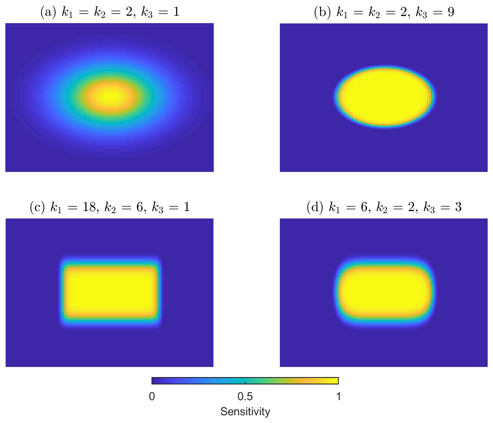
Figure 4(a) Standard 2-D Gaussian function. It is both a rotating super Gaussian with an exponent of 2 and a 2-D super Gaussian function with the x and y direction exponents equal to 2. (b) Rotating super Gaussian with an exponent (2×k3) of 18. (c) 2-D super Gaussian function with an exponent of 18 in the x direction and an exponent of 6 in the y direction. (d) A hybrid case between a rotating super Gaussian and a 2-D super Gaussian, featuring rounded corners. In all cases, FWHM. The grid size is 5 % of FWHMy.
The projection of a rectangular FOV for imaging grating spectrometers like OMI on the surface at large viewing angles leads to distorted quadrilateral footprints, as shown by the polygon ABCD in Fig. 5a. To account for this effect, a geometric transformation function is determined by the OMI pixel corner points (ABCD in Fig. 5a) and the corresponding rectangle (A′B′C′D′ in Fig. 5b) defined by the distances between the middle points of opposing edges of the OMI pixel quadrilateral. The spatial response function is first calculated according to Eq. (5) with FWHMx = and FWHMy = as shown in Fig. 5b and then projected to match the OMI pixel corners ABCD (Fig. 5a) using the geometric transformation function. This algorithm is implemented using both the OpenCV library in Python and the Image Processing Toolbox in MATLAB.
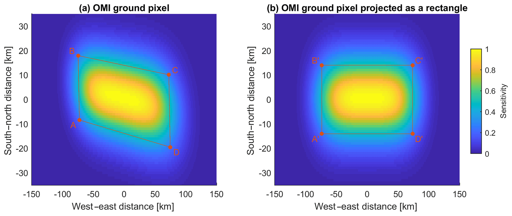
Figure 5(a) OMI pixel corners (ABCD) for across-track position 60 out of 1–60 and spatial response function with k1=4, k2=2, and k3=1. (b) The same OMI pixel transformed to a rectangle () and the corresponding transformed spatial response function. The horizontal and vertical axes are in different scales to demonstrate that the OMI pixel is not exactly a parallelogram. As a result, the geometric transformation function is projective (not exactly affine).
The proposed oversampling approach represents each satellite observation as a sensitive distribution, instead of a point or a polygon. If the true satellite spatial response function is used as the sensitive distribution, this approach is the theoretically optimal solution to the oversampling problem, and is hence referred to as “physical oversampling” hereafter. It follows the same equations as the tessellation approach as in Eqs. (1)–(4), except that the fractional overlapping area S(i,j) is generalized to the integration of the spatial response function of satellite observation i, , over the grid cell j:
where the denominator is the grid cell area. Similar to the tessellation approach, S(i,j) is always a dimensionless number between 0 and 1. By normalizing the grid cell area, this accurate form of S(i,j) can be directly replaced by approximating values such as evaluated at the grid center. is just the normalized spatial response function for observation i so that its spatial integration is unity. If the spatial response is uniform inside the pixel polygon and zero outside the polygon, this integration of the spatial response function within the grid cell is equivalent to the fractional overlapping area used in the tessellation approach. As such, the tessellation is just the extreme case where the spatial response function is a perfect 2-D boxcar. This corresponds to and in Eq. (5).
This physical oversampling approach can also be considered as a spatial interpolation method as discussed in Sect. 3.1 because the spatial response function can be defined beyond the satellite pixel boundaries and theoretically on the entire 2-D space. Moreover, instead of the exact form of spatial response function, the satellite observations can be represented by similar (with the same FWHM) but smoother sensitivity distributions to enhance the quality of the oversampling results. This possibility will be demonstrated in Sect. 5.2.
4.2 Balancing the errors from tessellation and discretization of spatial response
The tessellation approach is perfect if the spatial response of satellite observation is a boxcar, but otherwise it will introduce some error in the oversampled results (referred to as “tessellation error” hereafter). When the satellite spatial response function is smooth (instead of a boxcar), the exact solution is to calculate S(i,j) as the integration of the spatial response of satellite observation i over the area covered by the target grid cell j (Eq. 10). It is computationally demanding to numerically integrate the spatial response of all satellite pixels over each grid cell. To simplify it, one may discretize the spatial response function to the target oversampling grid and use the spatial response value at the grid center to approximate the integration. As such, the spatial response function only needs to be evaluated once per pixel per grid cell. To improve this simple discretization scheme, we calculate a weighted average of the spatial response values at the grid center and grid corners (Yang and Wolfe, 2001). Because the grid corners are shared by neighboring grid cells, this approach only doubles the spatial response calculation but significantly reduces the error induced by discretization (“discretization error” hereafter). Appendix B gives a detailed comparison of different discretization schemes.
The satellite sensors have very different spatial responses. The target grid size for level 3 data ranges from 0.25∘ (∼25 km) for many global operational products to 0.01∘ (∼1 km) for regional oversampling. The discretization error decreases as the size of the target grid cells becomes finer and the spatial response of satellite observations becomes better resolved. At any fixed target grid size, spatial response functions with smoother edges are better approximated by the discretization scheme. As such, it is essential to balance the tessellation and discretization errors based on the target grid cell size and the smoothness of the satellite spatial response so that the most accurate and efficient approximating method can be chosen.
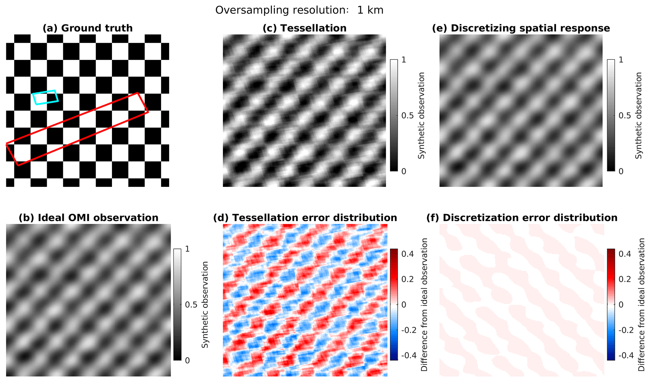
Figure 6Oversampling a synthetic checkerboard pattern, shown in panel (a), at a spatial scale smaller than the OMI pixels to a grid size of 1 km. The pattern in panel (a) is the ground truth of the concentration distribution. The ideal OMI observation in panel (b) is generated using spatial response function defined in Fig. 5 at very fine grids and then co-added back to 1 km. The pattern in panel (b) represents the ideal observation by OMI because no errors are introduced during the oversampling process. Panel (c) shows the result from the tessellation method (assuming S(i,j) is equal to the overlapping area between satellite pixel i and grid cell j). Panel (d) shows the difference between tessellation and the ideal observation. The values in panel (d) are equal to the values in panel (c) minus the values in panel (b). Panels (e, f) show the oversampling result by discretizing the spatial response function and its difference from the ideal observation. The values in panel (f) are equal to the values in panel (e) minus the values in panel (b).
Figure 6 compares the tessellation and discretization errors when oversampling synthetic OMI observations to a grid of 1 km (∼0.01∘). A checkerboard pattern is used as the “true” concentration distribution (alternating values of zeros and ones with a spatial period of 20 km × 20 km, as shown in Fig. 6a; it also shows OMI pixel polygons at across-track position no. 1 in red and across-track position no. 30 in cyan). Synthetic OMI observations are generated by sampling the checkerboard pattern using the OMI spatial response function, simplified using Eq. (8) with k1=4, k2=2 and discretized at a very fine grid (0.05 km, or ∼0.0005∘) so that the spatial response distribution is always fully resolved. The locations of OMI observations are from the real OMI NO2 products (Krotkov et al., 2017), filtered by cloud fraction <25 % and solar zenith angle <75∘ for 2005–2006. Instead of NO2 columns, the synthetic OMI observations at these locations are oversampled. The oversampled area is in the north midlatitude (∼40∘Ṅ). In Fig. 6b, the oversampling is conducted at a native grid size (0.05 km), and then the result is block-averaged to the 1 km target grid size to represent ideal OMI observations, as in Eq. (10). One should note that this discretization at 0.05 km is used to get the true map of OMI observation where the discretization error is negligible. It is unnecessary to oversample at this fine grid in general. Figure 6c and e show the results for tessellation and discretization of the spatial response at 1 km grid, where S(i,j) is approximated by fractional overlapping area and the discretization scheme, respectively. They both reproduce the checkerboard pattern in general, but the tessellation method generates errors up to 40 % (Fig. 6d) relative to the peak-to-trough value of the ideal observation because the OMI spatial response is smooth (Fig. 5) instead of boxcar. In contrast, the discretization error is much smaller (Fig. 6f) because of the small size of the target grid cells (1 km).
The analysis for Fig. 6 is repeated for a range of target grid sizes (1–50 km, or about 0.01–0.5∘) and different smoothness of the spatial response functions using the same OMI observation locations. The spatial response function is assumed to be 2-D super Gaussian (Eq. 8). The exponent in the along-track direction (k2) is tuned from 2 to 64, whereas the exponent in the across-track direction (k1) is set to be 2×k2. Figure 7a shows, for satellite observations with a quadrilateral FOV, the contour of the ratio between the discretization error and the tessellation error, calculated as the root-mean-squares of the differences between the ideal observation and the simplifications using tessellation and spatial response discretization, respectively. The contour line of unity divides the regimes where tessellation and discretization errors are dominant: discretization of the spatial response is more accurate for fine-grid oversampling of satellite observations with smooth spatial responses (small k1 and k2); tessellation is more accurate for coarser target grids and sharper spatial responses. Tessellation is perfect if k1 and k2 both approach infinity. The case of OMI (k1=4, k2=2) lies at the left edge (red vertical dashed line in Fig. 7a), and its intersect with the unity contour line is located at the target grid size of ∼16 km. In other words, it is beneficial to explicitly consider the spatial response of OMI observation for target oversampling grids finer than ∼16 km (about 0.15∘).
Similarly, Fig. 7b shows the ratios between discretization and tessellation errors for satellite observations with circular FOVs. The pixel dimensions and locations of IASI observations for 2015–2016 are used with standard data screening, and the spatial response function is assumed to be a rotating super Gaussian (Eq. 9). The exponential term (equal to 2×k3) varies from 2 to 64. When characterizing the IASI spatial response as a rotating super Gaussian function, the exponent is about 18, intersecting the unity contour line at the target grid size of ∼2 km. If the IASI instrument had the same spatial response as CrIS (the exponent is about 8), the intersect would be at the target grid size of ∼4 km. The results would be very similar when using the CrIS observation locations instead of IASI because the exact locations of any observations are averaged out and the IASI and CrIS pixel sizes are similar.
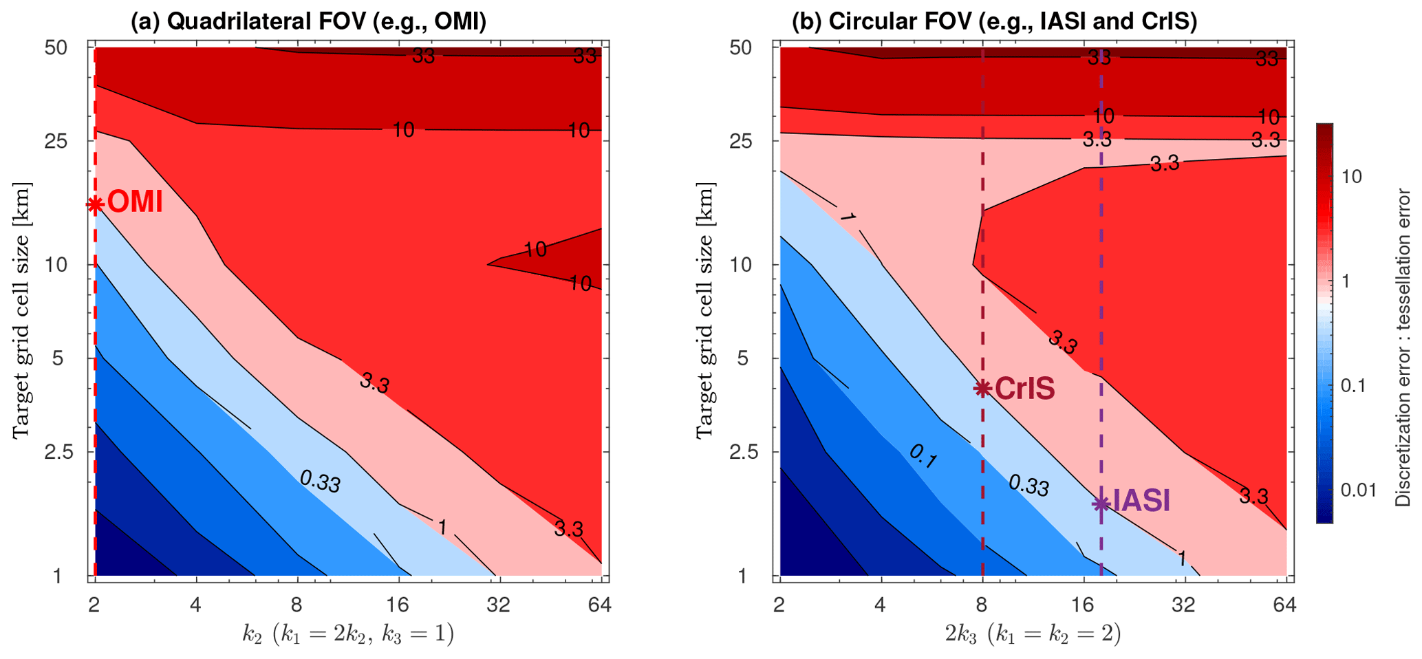
Figure 7(a) The ratio between discretization and tessellation errors for different combinations of spatial response function shapes and target grid size. The unity contour line delineates the regime where the tessellation error is larger than the discretization error (blueish contours) and the regime where the discretization error is larger than tessellation error (reddish contours). The red vertical dashed line indicates the approximate spatial response for OMI. The red star marks the threshold target grid size where the tessellation and discretization errors are equal for OMI. (b) Similar to panel (a) but the IASI pixel shapes and locations are used instead of OMI. The spatial response function exponents for CrIS and IASI and their intersects with the unity contour line are marked.
As shown by Fig. 7, the balance between tessellation and discretization errors depends on both the target grid size and the deviation of satellite spatial response function from an ideal 2-D boxcar shape. The uncertainty in the knowledge of the spatial response functions is not considered here, but the spatial response function can be characterized prelaunch and validated on orbit (Schreier et al., 2010; Sihler et al., 2017; de Graaf et al., 2016). For all three cases, the tessellation error significantly outweighs the discretization error at 1 km oversampling grid size by a factor of 4 for IASI and over 200 for OMI. Therefore, we recommend discretization of the spatial response function at a 1 km (or 0.01∘) grid for regional scale oversampling of OMI, IASI, and CrIS data and then co-adding to coarser grids if necessary. The threshold grid size where tessellation and discretization errors balance also depends on the ground size of satellite FOV. For the OMI successor missions with significantly smaller pixels (e.g., TROPOMI, TEMPO), the threshold grid size is expected to be finer.
4.3 Spatial resolution and spatial sampling
The difference between resolution and sampling density for 1-D spectral data has been thoroughly discussed in the literature (Chance et al., 2005). However, for 2-D, spatially resolved data, it is common to refer to both the sizes of the level 2 pixels and the size of the level 3 grid as the spatial “resolution” of the data. To avoid confusion, it is emphasized here that the true spatial resolution is limited by the sizes of level 2 pixels. The size of level 3 grid only determines the density of spatial sampling, which does little to enhance the true resolving power of the data after reaching a certain point. For example, the oversampling results using synthetic OMI data at 1 vs. 0.05 km grids are very similar (Fig. 6). Nonetheless, it is still beneficial to oversample, i.e., make level 3 grid size significantly smaller than level 2 pixel sizes, as demonstrated by Fig. 8. As the ground truth, an array of 2-D Gaussian functions are generated with FWHM ranging from 1 to 16 km (the second column of Fig. 8) and peak height of unity, and this true field of concentration is measured by an imaginary sensor whose spatial response function is a 2-D super Gaussian (Eq. 8) with FWHM = 10 km and (the first column and the white boxes inserted in the third column). The third column shows the oversampling results using 10 000 randomly located observations. The fine structures in the ground truth are clearly smoothed, limited by the spatial resolution that is inherent to the level 2 pixel sizes (10 km). However, by oversampling at a fine grid (0.2 km for the first row vs. 5 km for the second row), the spatial gradients are better recovered, and spatial features finer than individual level 2 pixels can be identified. Additionally, the details in the spatial response function is better resolved with a finer target grid, which is particularly beneficial when collocating with higher resolution measurements (e.g., a cloud imager). As such, although the spatial resolving power is ultimately determined by the spatial extent of satellite pixels, the physical oversampling approach helps in enhancing the visualization of spatial gradient and the identification of emission sources.
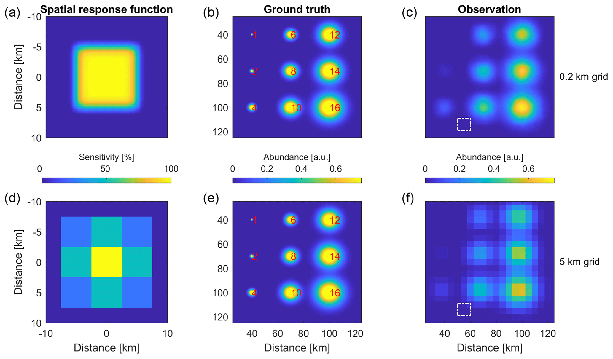
Figure 8First column: spatial response function of an imaginary sensor discretized at 0.2 km (a–c) and 5 km (d–f) grids. Second column: ground truth spatial distribution generated as an array of 2-D Gaussian functions of same height (the top and bottom panels are the same). The FWHM of each Gaussian is labeled. Third column: physical oversampling results using 10 000 randomly generated observations and discretized at 0.2 km (a–c) and 5 km (d–f) grids. The pixel size, which determines the spatial resolution, is labeled as the inserted white boxes.
5.1 Physical oversampling using OMI data
Figure 9 compares the drop-in-the-box method, point oversampling, tessellation, and physical oversampling using OMI NO2 tropospheric vertical column density (TVCD) within a 200 km × 200 km square centered around a power plant in Arizona. The first column shows the simple drop-in-the-box method on a 10 km grid. The second column averages OMI observations within a 12 km radius of each grid center. These two approaches assume OMI observations as points without consideration of pixel geometry and retrieval uncertainties. The third column shows results using the tessellation approach, and the fourth column shows the physical oversampling using the OMI spatial response functions as a 2-D super Gaussian function with k1=4 and k2=2. The target grid size is 1 km for the last three approaches. The first and third rows show the oversampled results (C(j) in Eq. 1) using 5 days (1–5 July 2005) and 5 months (May–September 2005) of data, respectively. The second and fourth rows show the corresponding numbers of pixels included in the averaging for each grid cell (D(j) in Eq. 4). For the drop-in-the-box approach, the total number of satellite observations included for each grid cell is much smaller and shown with a different color scale for the 5-month averaging.
The drop-in-the-box approach shows significant data gaps (5-day averaging) and high level of noise (5-month averaging), even when its target grid is 10 times coarser than the other oversampling approaches. There are two gaps where no observation is available for point oversampling over the 5 days (column 2, rows 1–2 in Fig. 9), which is an example of false negatives as these gaps are actually covered by OMI pixels (column 3, rows 1–2 in Fig. 9). The physical oversampling in the fourth column consistently shows the smoothest results with clear identification of the point source at the center of the domain, because the spatial response function of OMI is properly incorporated. The oversampled NO2 TVCD is biased high for the point oversampling approach because all observations within the averaging radius are averaged equally, but larger observation values generally are associated with larger uncertainties. The results from tessellation become increasingly similar to those from physical oversampling for longer averaging times, because the tessellation error is randomly distributed and will eventually be averaged out. The physical oversampling also does not require more computational resources than point oversampling and tessellation, making it suitable for a wide range of spatial scales and target grids.

Figure 9Level 3 results using the drop-in-the-box method (10 km grid, a, e, i, m), point oversampling (averaging radius: 12 km, 1 km grid, b, f, j, n), tessellation (pixel corners from the OMPIXCOR product, 1 km grid, c, g, k, o), and physical oversampling (2-D super Gaussian with k1=4 and k2=2, 1 km grid, d, h, l, p). The domain size is 200 km × 200 km. The first and third rows show the oversampled NO2 TVCD for 5 days and 5 months, and the second and fourth rows show the corresponding numbers of OMI observations used in the averaging for each grid cell. Note that panel (m) is on a different color scale than the other panels in the same row.
5.2 Physical oversampling using IASI data with smoother spatial sensitivity distributions
Although the physical oversampling using the true satellite spatial response functions produces the optimal estimation, the result is sometimes noisy and even unphysical, especially when the observations are noisy and sparse. In these cases, some spatial interpolation or smoothing methods are often needed. In addition to the specialized interpolation and smoothing methods discussed in Sect. 3.1, some smoothing can be applied within the oversampling framework. For example, the level of smoothing can be adjusted by the averaging radius in the point oversampling approach. Barkley et al. (2017) used a Gaussian filter to smooth tessellation results for OMI HCHO and CHOCHO products. When using the generalized 2-D super Gaussian function to characterize the satellite spatial response function (Eq. 5), it is also simple to tune the exponents (k3 in the cases of circular FOVs such as IASI and CrIS and k1 and k2 in the cases of quadrilateral FOVs such as OMI) so that the assumed satellite spatial sensitivity distribution is smoother than the true spatial response function. This often leads to better visualization and identification of local hot spots, especially for products with a high noise level or sparse spatial sampling. The advantage of this approach is that the smoothing is applied at the satellite pixel level (level 2) instead of grid level (level 3), so the geometry and error information for each satellite observation are preserved.
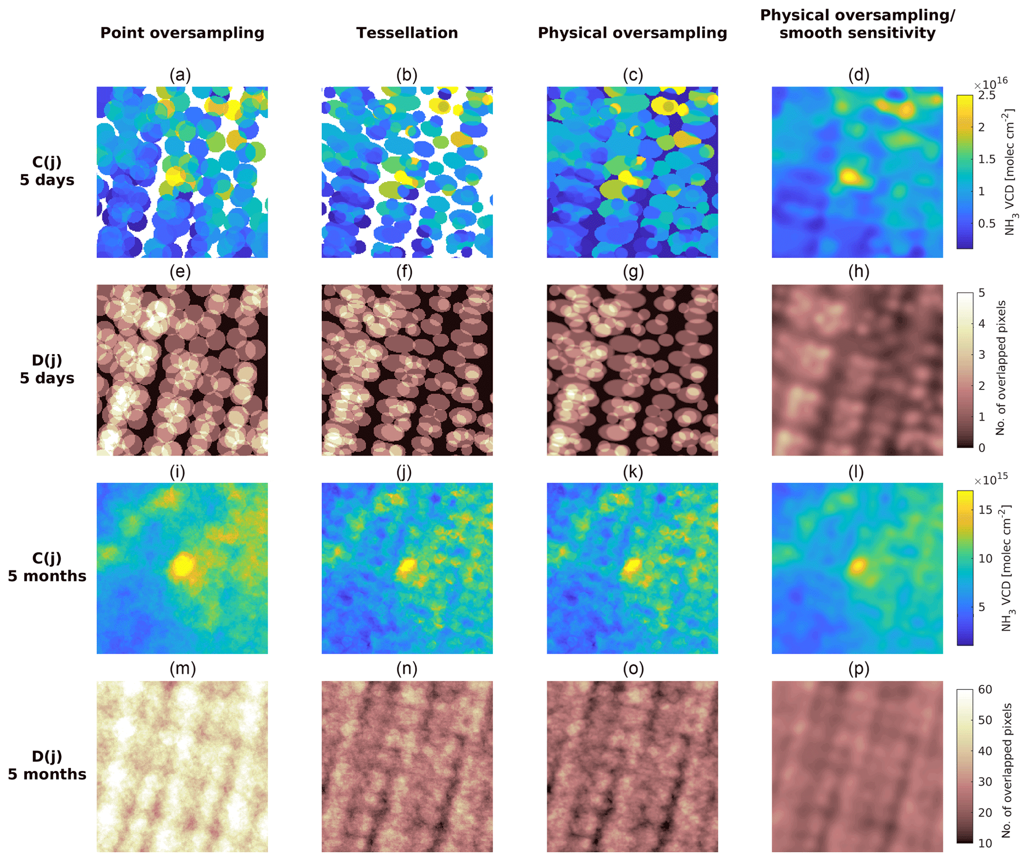
Figure 10Similar to Fig. 9 using IASI NH3 total column product for 2015. The drop-in-the-box approach is not included. Instead, the physical oversampling results using a smoother version of the IASI spatial response function are shown in panels (d, h, l, p). The true IASI spatial response function has much sharper edges than OMI, such that the physical oversampling results (c, g, k, o) are very similar to tessellation results (b, f, j, n).
Figure 10 shows similar oversampling results as Fig. 9, but using IASI NH3 total column density data (Van Damme et al., 2017) for 2015 in eastern Colorado, centered around a large cattle feedlot. The drop-in-the-box approach is not shown for IASI. The results from point oversampling, tessellation, and physical oversampling to a 1 km grid are presented in the first three columns. The true IASI spatial response functions have rather sharp edges (see Appendix A), so the physical oversampling shown in the third column of Fig. 10 is very similar to tessellation shown in the second column. Although this is the optimal estimation based on the physics of IASI observation, the spatial gradients are hard to identify for 5-day averaging and noisy for 5-month averaging. Instead of applying smoothing after the oversampling process, the fourth column uses a smooth spatial sensitivity distribution of a 2-D standard Gaussian function (2k3=2, rather than the true IASI spatial response function with 2k3∼18). As illustrated by the first row in Fig. 10, the physical oversampling using smoother spatial sensitivity distributions provides the best results by clearly identifying the central point source using only sparse (5-day) data. The third row in Fig. 10 demonstrates that with 5 months of averaging, the local NH3 gradients are well resolved. The point oversampling using a 12 km radius overly smooths the results, making the central hot spot artificially larger, whereas the general spatial gradients are still noisy (column 1, row 3). The overall number of IASI observations used in point oversampling is also significantly higher than tessellation and physical oversampling, as shown by the fourth row. This is because the 12 km averaging circle is much larger than most IASI footprints, and hence many IASI observations are double counted as false positives. The smoothing based on physical oversampling is much more effective in suppressing the noise, and the spatial gradients are adequately preserved (column 4, row 3). This is because each satellite FOV keeps the same FWHM and overall weight, and only the distribution of sensitivity becomes more spread out.
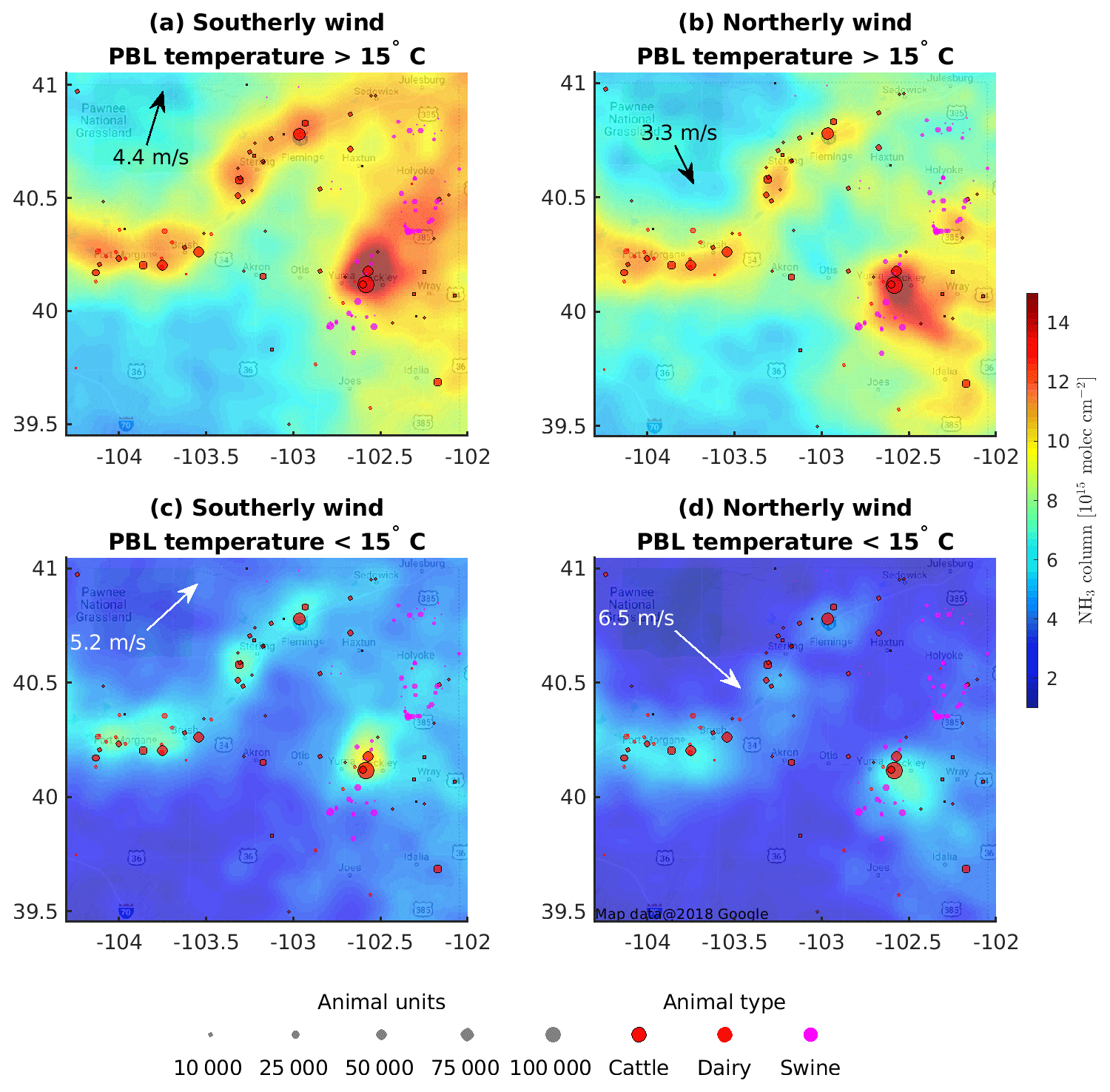
Figure 11Physical oversampling results using IASI-A NH3 total columns under southerly wind (a, c) and northerly wind (b, d) and high PBL temperature (>15 ∘C, a, b) and low PBL temperature (<15 ∘C, c, d). The text arrows show the average wind speed and wind direction at the locations and times of all IASI observations in each category. The size and location of large CAFOs are overlaid.
Oversampling based on Eqs. (1)–(3) also provides a flexible way to categorize the results according to environmental and temporal variables. The conventional way is to save the averaging weights for each level 2 observation (i.e., the level 2G product, where level 2 pixels are assigned to points of the latitude and longitude grid), but the averaging weights can only be defined for a specific grid. When representing each level 2 observation as a spatial sensitivity distribution (the actual instrument spatial response function or a smoother version of it), A(j) and B(j) can be calculated at fine spatial and temporal grids and then aggregated spatially and/or temporally. The level 3 map C(j) is just the grid-by-grid ratio of the aggregated A(j) and B(j). Similarly, A(j) and B(j) can be calculated according to environmental variables such as wind and temperature at fine intervals and binned to coarser categories as needed. Figure 11 shows the physical oversampling of NH3 total column under southerly winds (meridional wind component >0, panels a and c) and northerly winds (meridional wind component <0, panels b and d) and high PBL temperature (>15 ∘C, panels a and b) and low PBL temperature (<15 ∘C, panels c and d). Here the PBL temperature is the average air temperature from the surface to the top of the PBL, weighted by pressure. The average wind speed and wind direction under each category are labeled in the corresponding panels. IASI-A daytime data from 2008 to 2017 over northeastern Colorado are included in the oversampling, and a 2-D standard Gaussian is used as the spatial sensitivity distribution to smooth the results. The 3-D wind field, atmospheric temperature, surface pressure, and PBL height are interpolated from the North American Regional Reanalysis (Mesinger et al., 2006) from their native resolutions of 32 km and 3 h to the IASI pixel locations and overpass time. Using the concentrated animal feeding operation (CAFO) locations (colored dots; data courtesy of Daniel Bon, Colorado Department of Public Health and Environment) as a spatial reference, the downwind dispersion of the total NH3 column under different wind directions is clearly seen. The close match between large cattle CAFOs and the NH3 hot spots seen from space confirms that they are the dominant source of atmospheric NH3 in this region. The overall abundance of NH3 is significantly higher at warmer temperatures, in agreement with the previous in situ quantification of CAFO NH3 emissions in the same region (Sun et al., 2015b).
A physics-based approach is developed to oversample diverse satellite observational products to high-resolution destination grids. It represents each FOV as a sensitivity distribution on the ground, which is physically a more realistic representation of satellite observations. This sensitivity distribution can be determined by the spatial response function of each satellite sensor. We propose a generalized 2-D super Gaussian function that can standardize the spatial response functions of many satellite sensors with distinct observation mechanisms and viewing geometries. This generalized 2-D super Gaussian function can be reduced to a rotating super Gaussian to characterize the circular FOV of IASI and CrIS or a 2-D super Gaussian to characterize the quadrilateral FOV of OMI and its successors. It can also represent hybrid cases where the FOV is quadrilateral but with rounded corners. When the shape-determining exponents in the generalized 2-D super Gaussian function approach infinity, the FOV is equivalent to a polygon, as assumed in the tessellation approach.
Synthetic OMI and IASI observations were generated assuming the spatial response functions are perfectly known to compare the tessellation error and the discretization error. The balance between these two error sources depends on the target grid size, the ground size of FOV, and the smoothness of spatial response functions. The proposed oversampling approach is generally more accurate for fine-grid oversampling of satellite observations with smooth spatial responses, whereas tessellation is more accurate for coarse grids and sharper spatial responses. For OMI, CrIS, and IASI, the threshold target grid size where both errors are equal are at ∼16, ∼4, and ∼2 km, respectively. Therefore, it is recommended to oversample to 1 km (0.01∘) and then co-add to coarser grids if necessary for regional studies. The tessellation may be more desirable for generating global level 3 products with coarse grids. The generalized 2-D super Gaussian function also enables smoothing of the level 3 results by decreasing the shape-determining exponents, useful for high noise levels or sparse satellite datasets. This smoothing performed at each observation is more physically realistic than arbitrarily tuning the averaging radius and the spatial filtering of the level 3 map as the weightings of level 2 pixels are unchanged.
The new physical oversampling approach is applied to OMI NO2 products and IASI NH3 products, showing substantially improved visualization of trace gas distribution and local gradients. With proper consideration of the spatial response functions, this approach can be applied to multiple previous, current, and future satellite datasets, which will help to create long-term consistent data records for atmospheric composition.
A MATLAB implementation of the physical oversampling is available at https://github.com/Kang-Sun-CfA/Oversampling_matlab/, last access: 5 December 2018 (Sun, 2018).
The spatial response functions of IASI are tabulated at https://iasi.cnes.fr/en/IASI/A_caract_instr.htm, last access: 10 December 2017, for each of its four detector pixels. They are very close to ideal circular FOV with some smoothing at the edge and weak non-homogeneity at the top response, as shown by Fig. A1.

Figure A1IASI spatial response functions (also known as point spread functions) defined at the viewing angular space. The corresponding ground distance at nadir is shown in the axis on the right. The IASI orbit height is assumed to be 817 km above the ground.
Figure A2 shows a rotating super Gaussian function (Eq. 9) fitted to the tabulated spatial response function at detector pixel no. 2 and the fitting residual. With only two parameters (the width and exponent of the super Gaussian), the spatial response function can be well reconstructed by the rotating super Gaussian function.
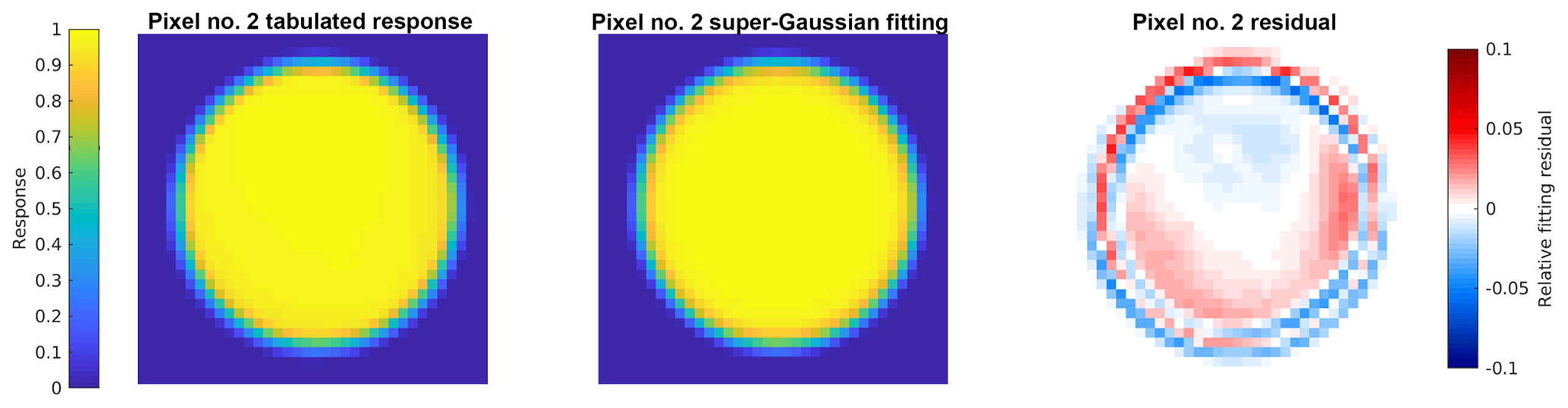
Figure A2Fitting a tabulated IASI spatial response function for pixel no. 2 using rotating super Gaussian. The fitted exponent is 18.5.
Figure A3a shows the fitting of the across-track cross section of the spatial response function of IASI detector pixel no. 2 using a 1-D super Gaussian function. The FWHM is 11.6 km on the ground and the exponent is ∼18. The detailed information on the spatial response of CrIS detectors is proprietary, but Wang et al. (2013) provides the spatial response values at a few angles; i.e., the angles of 1.2380, 1.1000, 0.9420, and 0.8735∘ correspond to 3 %, 10 %, 50 %, and 70 % of the peak response. Based on this information, a 1-D super Gaussian can be fitted with FWHM=13.6 km on the ground and an exponent of 7.93, as shown by Fig. A3b. The CrIS orbit height is assumed to be 824 km above the ground.
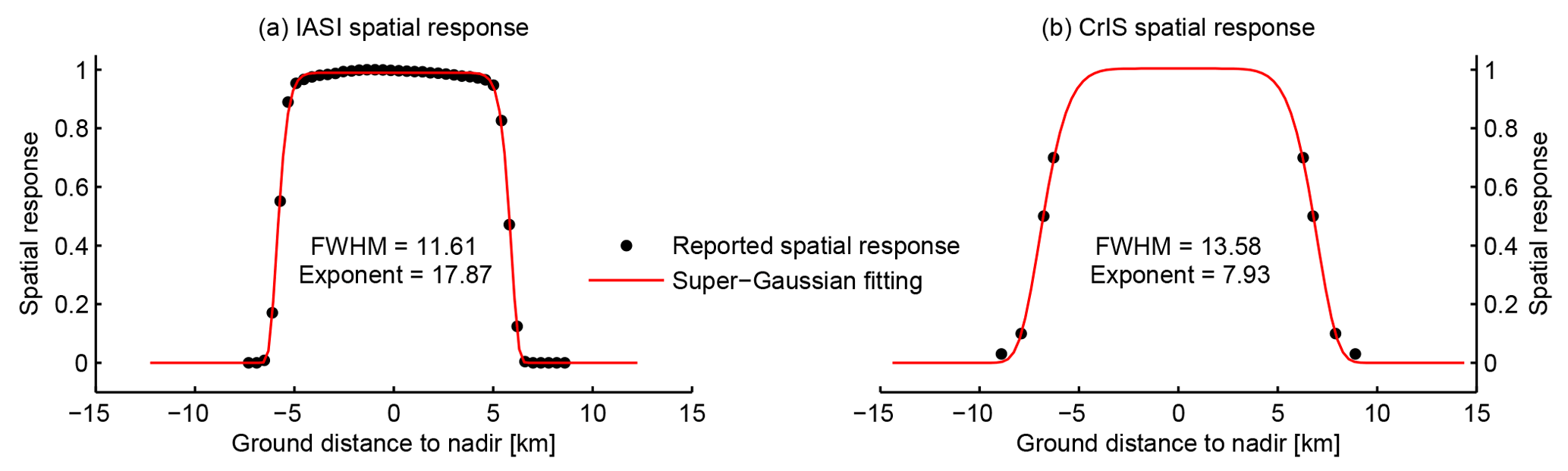
Figure A3Slices of spatial response functions for IASI (a) and CrIS (b). Super Gaussian functions are fitted with the exponent ∼18 for IASI and ∼8 for CrIS. The spatial response functions are projected on ground to reflect actual nadir pixel sizes.
To compare different discretization schemes, we first construct an ideal spatial response function using OMI pixel boundaries but sharper edges (k1=12, k2=6, see Fig. B2a) and zoom in to a single grid cell of 5 km × 5 km (Fig. B1a). The true value of S(i,j) should be the integration of the spatial response function over the grid cell area as in Eq. (10). A simple discretization scheme is to use the spatial response value at the grid center, C (Fig. B1b):
where S(C) denotes the evaluation of continuous spatial response function S(x,y) at the coordinates of the grid center C. A more advanced discretization scheme is to calculate the spatial response values at both the grid center and the grid corners ABDE (Fig. B1c) and approximate the integration as the sum of the volumes of four triangular prisms (i.e., ABC, BDC, DEC, and EAC):
Hence it is a weighted average with the weight for grid center twice that of the weight for grid corners. For completeness, the assumption of tessellation is also shown in Fig. B1d, where spatial response is assumed to be unity inside the pixel boundary and zero outside. S(i,j) is calculated as the fractional area covered by the portion of pixel polygon within the grid cell.
In Fig. B2, both discretization schemes and tessellation are applied to calculate S(i,j) for all grid cells near the satellite FOV. Figure B2b–d shows the distribution of errors from these three approximation methods, where the true S(i,j) is the numerical integration of the high-resolution spatial response function shown in Fig. B2a. The errors in both discretization schemes (discretization only at grid center, Fig. B2b, and weighted averaging of grid center and grid corners, Fig. B2c) and the tessellation error are shown as the root-mean-square of the error distribution. The discretization scheme using both grid center and grid corner values significantly reduces the error, which in this case is also lower than the tessellation error. For a realistic OMI spatial response function (k1=4, k2=2), the discretization errors in both cases are significantly lower than the tessellation error at this grid size (5 km).
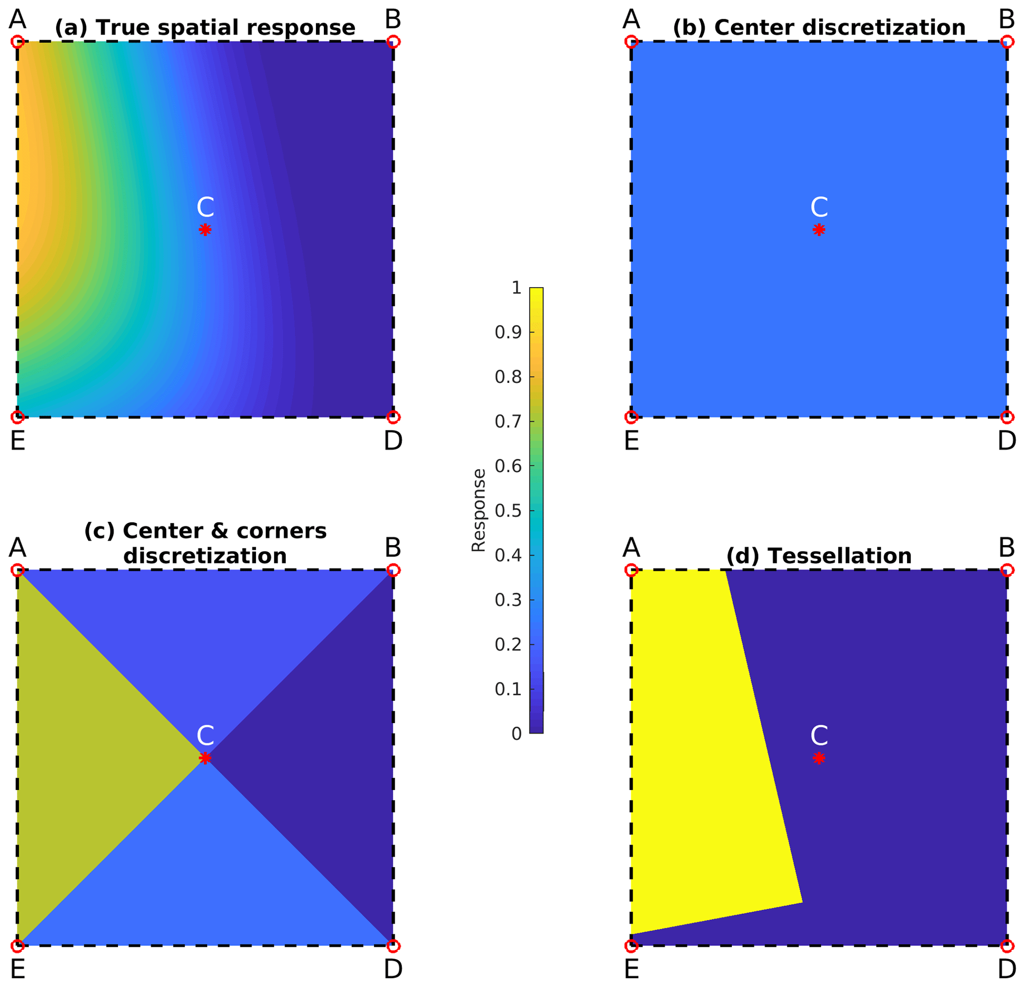
Figure B1(a) An ideal spatial response function constructed using OMI across-track no. 30 pixel boundary and relatively sharp edges (k1=12, k2=6, k3=1). Only the overlapping portion with a 5 km × 5 km grid cell (square ABDE) is shown. C is the grid center. (b) Simple discretization scheme, where the grid cell value is approximated by the spatial response at central position C. (c) The spatial response is discretized at both grid center and grid corners. See text for details. (d) Tessellation, where the spatial response is assumed to be unity inside the pixel boundary and zero outside. The polygons are color-coded by the spatial response values.
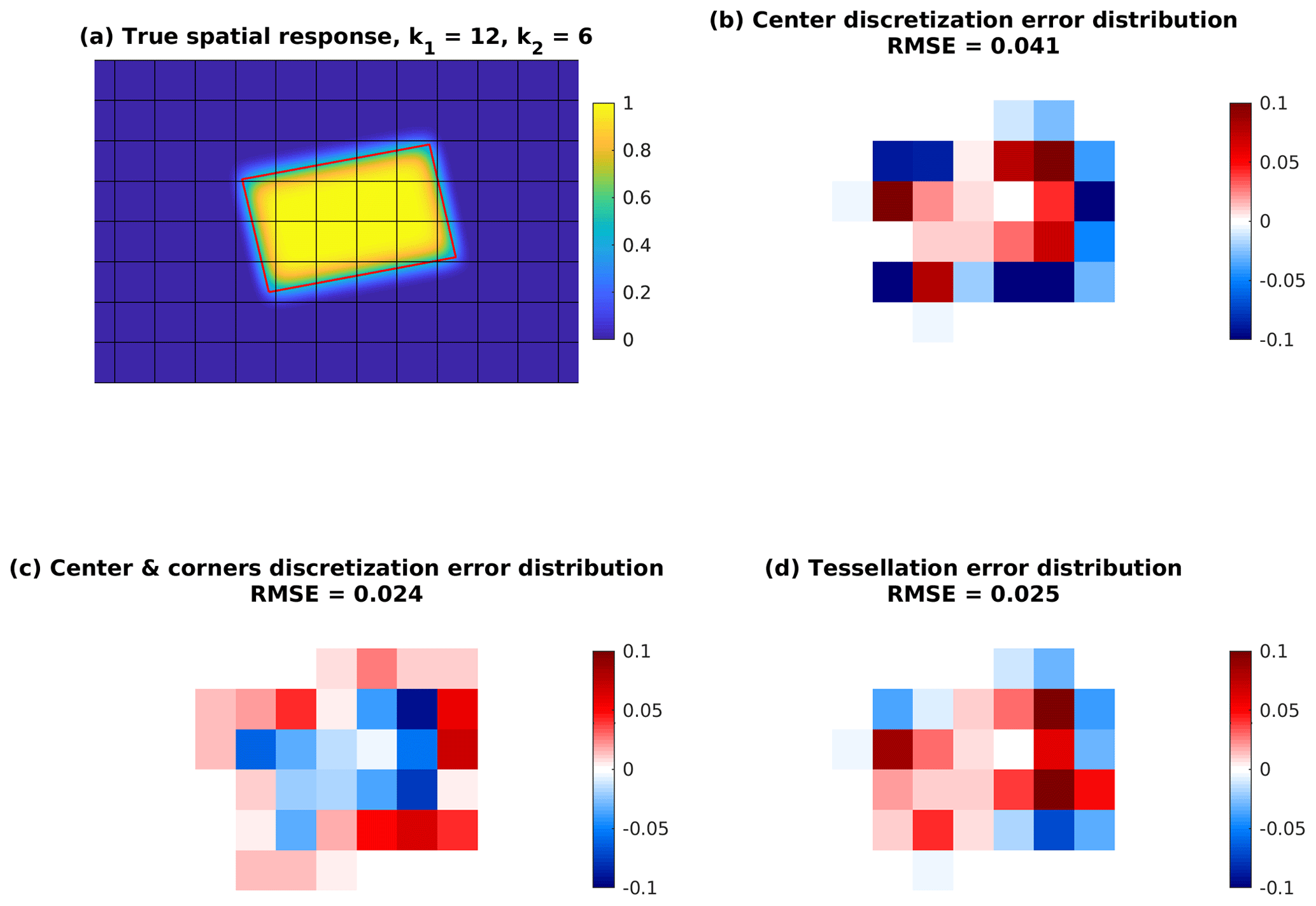
Figure B2(a) An ideal spatial response function constructed using OMI across-track no. 30 pixel boundary (red rectangle) and relatively sharp edges (k1=12, k2=6, k3=1). The destination grid of 5 km × 5 km is also shown. (b) Errors induced by discretization only at grid centers (discretized values − true values). The true value for each 5 km × 5 km grid is calculated by numerical integration using the high-resolution spatial response shown in panel (a). (c) Errors induced by discretization at both grid centers and grid corners. (d) Tessellation errors. RMSE is the root-mean-square of the error distribution.
KS, LZ, KY, and GH developed and implemented the oversampling algorithms. KCP provided expertise on the CrIS instrument and products. CCM, KC, GGA, and XL provided expertise on the OMI instrument and products. LC, PFC, MVD, and MZ provided expertise on the IASI instrument and products. KS collected the data, analyzed the results, and wrote the manuscript. All authors contributed to interpretations and edited the manuscript.
The authors declare that they have no conflict of interest.
We acknowledge support from NASA (sponsor contract numbers NNX14AF16G and NNX14AF56G), the RENEW
Institute and School of Engineering and Applied Science at the University at
Buffalo, and Smithsonian Institution subaward SV8-8802. We thank John Houck
at the SAO; Thomas Kurosu at JPL; Holger Sihler at MPI-C; Glen Jaross at
NASA; Rui Wang, Xuehui Guo, and Da Pan at Princeton University; and Likun Wang
at University of Maryland for helpful discussions. We thank the OMI
science team for making the OMI NO2 data available at
https://disc.gsfc.nasa.gov/datasets/OMNO2_V003/summary, last access: 1 July 2018, and the IASI science
team for making the IASI NH3 retrieval available at
http://iasi.aeris-data.fr/NH3, last access: 1 October 2018. Lieven Clarisse is a research associate with
the Belgian F.R.S-FNRS and acknowledges the support.
Edited by: Jun Wang
Reviewed by: two anonymous referees
Aumann, H. H., Chahine, M. T., Gautier, C., Goldberg, M. D., Kalnay, E., McMillin, L. M., Revercomb, H., Rosenkranz, P. W., Smith, W. L., Staelin, D. H., Strow, L. L., and Susskind, J.: AIRS/AMSU/HSB on the Aqua mission: design, science objectives, data products, and processing systems, IEEE T. Geosci. Remote, 41, 253–264, https://doi.org/10.1109/TGRS.2002.808356, 2003. a
Baek, B. H., Aneja, V. P., and Tong, Q.: Chemical coupling between ammonia, acid gases, and fine particles, Environ. Pollut., 129, 89–98, 2004. a
Bak, J., Liu, X., Kim, J.-H., Haffner, D. P., Chance, K., Yang, K., and Sun, K.: Characterization and correction of OMPS nadir mapper measurements for ozone profile retrievals, Atmos. Meas. Tech., 10, 4373–4388, https://doi.org/10.5194/amt-10-4373-2017, 2017. a
Barkley, M. P., González Abad, G., Kurosu, T. P., Spurr, R., Torbatian, S., and Lerot, C.: OMI air-quality monitoring over the Middle East, Atmos. Chem. Phys., 17, 4687–4709, https://doi.org/10.5194/acp-17-4687-2017, 2017. a
Beirle, S., Boersma, K. F., Platt, U., Lawrence, M. G., and Wagner, T.: Megacity emissions and lifetimes of nitrogen oxides probed from space, Science, 333, 1737–1739, 2011. a
Beirle, S., Lampel, J., Lerot, C., Sihler, H., and Wagner, T.: Parameterizing the instrumental spectral response function and its changes by a super-Gaussian and its derivatives, Atmos. Meas. Tech., 10, 581–598, https://doi.org/10.5194/amt-10-581-2017, 2017. a
Borsdorff, T., Aan de Brugh, J., Hu, H., Aben, I., Hasekamp, O., and Landgraf, J.: Measuring Carbon Monoxide With TROPOMI: First Results and a Comparison With ECMWF-IFS Analysis Data, Geophys. Res. Lett., 45, 2826–2832, https://doi.org/10.1002/2018GL077045, 2018. a
Bovensmann, H., Burrows, J., Buchwitz, M., Frerick, J., Noël, S., Rozanov, V., Chance, K., and Goede, A.: SCIAMACHY: Mission objectives and measurement modes, J. Atmos. Sci., 56, 127–150, 1999. a
Bowman, K. W., Rodgers, C. D., Kulawik, S. S., Worden, J., Sarkissian, E., Osterman, G., Steck, T., Lou, M., Eldering, A., Shephard, M., Worden, H., Lampel, M., Clough, S., Brown, P., Rinsland, C., Gunson, M., and Beer, R.: Tropospheric emission spectrometer: Retrieval method and error analysis, IEEE T. Geosci. Remote, 44, 1297–1307, https://doi.org/10.1109/TGRS.2006.871234, 2006. a
Buchwitz, M., de Beek, R., Burrows, J. P., Bovensmann, H., Warneke, T., Notholt, J., Meirink, J. F., Goede, A. P. H., Bergamaschi, P., Körner, S., Heimann, M., and Schulz, A.: Atmospheric methane and carbon dioxide from SCIAMACHY satellite data: initial comparison with chemistry and transport models, Atmos. Chem. Phys., 5, 941–962, https://doi.org/10.5194/acp-5-941-2005, 2005. a
Burrows, J. P., Weber, M., Buchwitz, M., Rozanov, V., Ladstätter-Weißenmayer, A., Richter, A., DeBeek, R., Hoogen, R., Bramstedt, K., Eichmann, K.-U., Eisinger, M., and Perner, D.: The global ozone monitoring experiment (GOME): Mission concept and first scientific results, J. Atmos. Sci., 56, 151–175, 1999. a
Chance, K., Kurosu, T. P., and Sioris, C. E.: Undersampling correction for array detector-based satellite spectrometers, Appl. Optics, 44, 1296–1304, 2005. a
Chan Miller, C., Gonzalez Abad, G., Wang, H., Liu, X., Kurosu, T., Jacob, D. J., and Chance, K.: Glyoxal retrieval from the Ozone Monitoring Instrument, Atmos. Meas. Tech., 7, 3891–3907, https://doi.org/10.5194/amt-7-3891-2014, 2014. a
Clarisse, L., Shephard, M. W., Dentener, F., Hurtmans, D., Cady-Pereira, K., Karagulian, F., Van Damme, M., Clerbaux, C., and Coheur, P.-F.: Satellite monitoring of ammonia: A case study of the San Joaquin Valley, J. Geophys. Res.-Atmos., 115, D13, https://doi.org/10.1029/2009JD013291, 2010. a
Clerbaux, C., Boynard, A., Clarisse, L., George, M., Hadji-Lazaro, J., Herbin, H., Hurtmans, D., Pommier, M., Razavi, A., Turquety, S., Wespes, C., and Coheur, P.-F.: Monitoring of atmospheric composition using the thermal infrared IASI/MetOp sounder, Atmos. Chem. Phys., 9, 6041–6054, https://doi.org/10.5194/acp-9-6041-2009, 2009. a, b
CNES: IASI Instrument Characteristics, available at: https://iasi.cnes.fr/en/IASI/A_caract_instr.htm (last access: 10 December 2017), 2015. a
Dammers, E., Shephard, M. W., Palm, M., Cady-Pereira, K., Capps, S., Lutsch, E., Strong, K., Hannigan, J. W., Ortega, I., Toon, G. C., Stremme, W., Grutter, M., Jones, N., Smale, D., Siemons, J., Hrpcek, K., Tremblay, D., Schaap, M., Notholt, J., and Erisman, J. W.: Validation of the CrIS fast physical NH3 retrieval with ground-based FTIR, Atmos. Meas. Tech., 10, 2645–2667, https://doi.org/10.5194/amt-10-2645-2017, 2017. a
de Foy, B., Krotkov, N. A., Bei, N., Herndon, S. C., Huey, L. G., Martínez, A.-P., Ruiz-Suárez, L. G., Wood, E. C., Zavala, M., and Molina, L. T.: Hit from both sides: tracking industrial and volcanic plumes in Mexico City with surface measurements and OMI SO2 retrievals during the MILAGRO field campaign, Atmos. Chem. Phys., 9, 9599–9617, https://doi.org/10.5194/acp-9-9599-2009, 2009. a
de Foy, B., Lu, Z., Streets, D. G., Lamsal, L. N., and Duncan, B. N.: Estimates of power plant NOx emissions and lifetimes from OMI NO2 satellite retrievals, Atmos. Environ., 116, 1–11, https://doi.org/10.1016/j.atmosenv.2015.05.056, 2015. a, b
de Graaf, M., Sihler, H., Tilstra, L. G., and Stammes, P.: How big is an OMI pixel?, Atmos. Meas. Tech., 9, 3607–3618, https://doi.org/10.5194/amt-9-3607-2016, 2016. a, b, c, d, e, f, g
Drummond, J. R., Zou, J., Nichitiu, F., Kar, J., Deschambaut, R., and Hackett, J.: A review of 9-year performance and operation of the MOPITT instrument, Adv. Space Res., 45, 760–774, https://doi.org/10.1016/j.asr.2009.11.019, 2010. a
Duncan, B. N., Lamsal, L. N., Thompson, A. M., Yoshida, Y., Lu, Z., Streets, D. G., Hurwitz, M. M., and Pickering, K. E.: A space-based, high-resolution view of notable changes in urban NOx pollution around the world (2005–2014), J. Geophys. Res.-Atmos., 121, 976–996, https://doi.org/10.1002/2015JD024121, 2016. a, b
Eldering, A., O'Dell, C. W., Wennberg, P. O., Crisp, D., Gunson, M. R., Viatte, C., Avis, C., Braverman, A., Castano, R., Chang, A., Chapsky, L., Cheng, C., Connor, B., Dang, L., Doran, G., Fisher, B., Frankenberg, C., Fu, D., Granat, R., Hobbs, J., Lee, R. A. M., Mandrake, L., McDuffie, J., Miller, C. E., Myers, V., Natraj, V., O'Brien, D., Osterman, G. B., Oyafuso, F., Payne, V. H., Pollock, H. R., Polonsky, I., Roehl, C. M., Rosenberg, R., Schwandner, F., Smyth, M., Tang, V., Taylor, T. E., To, C., Wunch, D., and Yoshimizu, J.: The Orbiting Carbon Observatory-2: first 18 months of science data products, Atmos. Meas. Tech., 10, 549–563, https://doi.org/10.5194/amt-10-549-2017, 2017. a
Fioletov, V., McLinden, C., Krotkov, N., Moran, M., and Yang, K.: Estimation of SO2 emissions using OMI retrievals, Geophys. Res. Lett., 38, 21, https://doi.org/10.1029/2011GL049402, 2011. a
Fioletov, V., McLinden, C. A., Kharol, S. K., Krotkov, N. A., Li, C., Joiner, J., Moran, M. D., Vet, R., Visschedijk, A. J. H., and Denier van der Gon, H. A. C.: Multi-source SO2 emission retrievals and consistency of satellite and surface measurements with reported emissions, Atmos. Chem. Phys., 17, 12597–12616, https://doi.org/10.5194/acp-17-12597-2017, 2017. a
Fioletov, V. E., McLinden, C. A., Krotkov, N., and Li, C.: Lifetimes and emissions of SO2 from point sources estimated from OMI, Geophys. Res. Lett., 42, 1969–1976, 2015. a
Geddes, J. A., Martin, R. V., Boys, B. L., and van Donkelaar, A.: Long-term trends worldwide in ambient NO2 concentrations inferred from satellite observations, Environ. Health Persp., 124, 281–289, https://doi.org/10.1289/ehp.1409567, 2016. a
González Abad, G., Liu, X., Chance, K., Wang, H., Kurosu, T. P., and Suleiman, R.: Updated Smithsonian Astrophysical Observatory Ozone Monitoring Instrument (SAO OMI) formaldehyde retrieval, Atmos. Meas. Tech., 8, 19–32, https://doi.org/10.5194/amt-8-19-2015, 2015. a
Han, Y., Revercomb, H., Cromp, M., Gu, D., Johnson, D., Mooney, D., Scott, D., Strow, L., Bingham, G., Borg, L., Chen, Y., DeSlover, D., Esplin, M., Hagan, D., Jin, X., Knuteson, R., Motteler, H., Predina, J., Suwinski, L., Taylor, J., Tobin, D., Tremblay, D., Wang, C., Wang, L., Wang, L., and Zavyalov, V.: Suomi NPP CrIS measurements, sensor data record algorithm, calibration and validation activities, and record data quality, J. Geophys. Res.-Atmos., 118, 12–734, https://doi.org/10.1002/2013JD020344, 2013. a
Hu, H., Landgraf, J., Detmers, R., Borsdorff, T., Aan de Brugh, J., Aben, I., Butz, A., and Hasekamp, O.: Toward Global Mapping of Methane With TROPOMI: First Results and Intersatellite Comparison to GOSAT, Geophys. Res. Lett., 45, 3682–3689, https://doi.org/10.1002/2018GL077259, 2018. a
Jacob, D. J., Turner, A. J., Maasakkers, J. D., Sheng, J., Sun, K., Liu, X., Chance, K., Aben, I., McKeever, J., and Frankenberg, C.: Satellite observations of atmospheric methane and their value for quantifying methane emissions, Atmos. Chem. Phys., 16, 14371–14396, https://doi.org/10.5194/acp-16-14371-2016, 2016. a
Kim, H. C., Lee, P., Judd, L., Pan, L., and Lefer, B.: OMI NO2 column densities over North American urban cities: the effect of satellite footprint resolution, Geosci. Model Dev., 9, 1111–1123, https://doi.org/10.5194/gmd-9-1111-2016, 2016. a
Kort, E. A., Frankenberg, C., Costigan, K. R., Lindenmaier, R., Dubey, M. K., and Wunch, D.: Four corners: The largest US methane anomaly viewed from space, Geophys. Res. Lett., 41, 6898–6903, 2014. a
Krotkov, N. A.: OMI/Aura NO2 Cloud-Screened Total and Tropospheric Column L3 Global Gridded V3, https://doi.org/10.5067/Aura/OMI/DATA3007, 2013. a
Krotkov, N. A., Lamsal, L. N., Celarier, E. A., Swartz, W. H., Marchenko, S. V., Bucsela, E. J., Chan, K. L., Wenig, M., and Zara, M.: The version 3 OMI NO2 standard product, Atmos. Meas. Tech., 10, 3133–3149, https://doi.org/10.5194/amt-10-3133-2017, 2017. a, b, c
Kuhlmann, G., Hartl, A., Cheung, H. M., Lam, Y. F., and Wenig, M. O.: A novel gridding algorithm to create regional trace gas maps from satellite observations, Atmos. Meas. Tech., 7, 451–467, https://doi.org/10.5194/amt-7-451-2014, 2014. a
Kurosu, T. P. and Celarier, E. A.: OMI/Aura Global Ground Pixel Corners 1-Orbit L2 Swath 13×24 km V003, https://doi.org/10.5067/Aura/OMI/DATA2020, 2010. a
Lamsal, L. N., Duncan, B. N., Yoshida, Y., Krotkov, N. A., Pickering, K. E., Streets, D. G., and Lu, Z.: US NO2 trends (2005–2013): EPA Air Quality System (AQS) data versus improved observations from the Ozone Monitoring Instrument (OMI), Atmos. Environ., 110, 130–143, 2015. a
Levelt, P. F., Joiner, J., Tamminen, J., Veefkind, J. P., Bhartia, P. K., Stein Zweers, D. C., Duncan, B. N., Streets, D. G., Eskes, H., van der A, R., McLinden, C., Fioletov, V., Carn, S., de Laat, J., DeLand, M., Marchenko, S., McPeters, R., Ziemke, J., Fu, D., Liu, X., Pickering, K., Apituley, A., González Abad, G., Arola, A., Boersma, F., Chan Miller, C., Chance, K., de Graaf, M., Hakkarainen, J., Hassinen, S., Ialongo, I., Kleipool, Q., Krotkov, N., Li, C., Lamsal, L., Newman, P., Nowlan, C., Suleiman, R., Tilstra, L. G., Torres, O., Wang, H., and Wargan, K.: The Ozone Monitoring Instrument: overview of 14 years in space, Atmos. Chem. Phys., 18, 5699–5745, https://doi.org/10.5194/acp-18-5699-2018, 2018. a, b
Li, C., Krotkov, N. A., Carn, S., Zhang, Y., Spurr, R. J. D., and Joiner, J.: New-generation NASA Aura Ozone Monitoring Instrument (OMI) volcanic SO2 dataset: algorithm description, initial results, and continuation with the Suomi-NPP Ozone Mapping and Profiler Suite (OMPS), Atmos. Meas. Tech., 10, 445–458, https://doi.org/10.5194/amt-10-445-2017, 2017a. a
Li, J. and Heap, A. D.: Spatial interpolation methods applied in the environmental sciences: A review, Environ. Modell. Softw., 53, 173–189, https://doi.org/10.1016/j.envsoft.2013.12.008, 2014. a
Li, Y., Thompson, T. M., Van Damme, M., Chen, X., Benedict, K. B., Shao, Y., Day, D., Boris, A., Sullivan, A. P., Ham, J., Whitburn, S., Clarisse, L., Coheur, P.-F., and Collett Jr., J. L.: Temporal and spatial variability of ammonia in urban and agricultural regions of northern Colorado, United States, Atmos. Chem. Phys., 17, 6197–6213, https://doi.org/10.5194/acp-17-6197-2017, 2017b. a
Liu, F., Beirle, S., Zhang, Q., Dörner, S., He, K., and Wagner, T.: NOx lifetimes and emissions of cities and power plants in polluted background estimated by satellite observations, Atmos. Chem. Phys., 16, 5283–5298, https://doi.org/10.5194/acp-16-5283-2016, 2016. a
Liu, X., Chance, K., Sioris, C. E., Kurosu, T. P., Spurr, R. J. D., Martin, R. V., Fu, T.-M., Logan, J. A., Jacob, D. J., Palmer, P. I., Newchurch, M. J., Megretskaia, I. A., and Chatfield, R. B.: First directly retrieved global distribution of tropospheric column ozone from GOME: Comparison with the GEOS-CHEM model, J. Geophys. Res.-Atmos., 111, D2, https://doi.org/10.1029/2005JD006564, 2006. a
Martin, R. V.: Satellite remote sensing of surface air quality, Atmos. Environ., 42, 7823–7843, 2008. a
McLinden, C. A., Fioletov, V., Boersma, K. F., Krotkov, N., Sioris, C. E., Veefkind, J. P., and Yang, K.: Air quality over the Canadian oil sands: A first assessment using satellite observations, Geophys. Res. Lett., 39, 4, https://doi.org/10.1029/2011GL050273, 2012. a, b
McLinden, C. A., Fioletov, V., Shephard, M. W., Krotkov, N., Li, C., Martin, R. V., Moran, M. D., and Joiner, J.: Space-based detection of missing sulfur dioxide sources of global air pollution, Nat. Geosci., 9, 496–500, 2016. a
Mesinger, F., DiMego, G., Kalnay, E., Mitchell, K., Shafran, P. C., Ebisuzaki, W., Jović, D., Woollen, J., Rogers, E., Berbery, E. H., Ek, M. B., Fan, Y., Grumbine, R., Higgins, W., Li, H., Lin, Y., Manikin, G., Parrish, D., and Shi, W.: North American Regional Reanalysis, B. Am. Meteorol. Soc., 87, 343–360, https://doi.org/10.1175/BAMS-87-3-343, 2006. a
Munro, R., Lang, R., Klaes, D., Poli, G., Retscher, C., Lindstrot, R., Huckle, R., Lacan, A., Grzegorski, M., Holdak, A., Kokhanovsky, A., Livschitz, J., and Eisinger, M.: The GOME-2 instrument on the Metop series of satellites: instrument design, calibration, and level 1 data processing – an overview, Atmos. Meas. Tech., 9, 1279–1301, https://doi.org/10.5194/amt-9-1279-2016, 2016. a
Paulot, F. and Jacob, D. J.: Hidden cost of U.S. agricultural exports: particulate matter from ammonia emissions., Environ. Sci. Technol., 48, 903–8, https://doi.org/10.1021/es4034793, 2014. a
Rodriguez, J. V., Seftor, C. J., Wellemeyer, C. G., and Chance, K.: An overview of the nadir sensor and algorithms for the NPOESS ozone mapping and profiler suite (OMPS), in: Optical Remote Sensing of the Atmosphere and Clouds III, International Society for Optics and Photonics, Hangzhou, China, 4891, 65–76, 2003. a
Russell, A. R., Valin, L. C., Bucsela, E. J., Wenig, M. O., and Cohen, R. C.: Space-based Constraints on Spatial and Temporal Patterns of NOx Emissions in California, 2005–2008, Environ. Sci. Technol., 44, 3608–3615, https://doi.org/10.1021/es903451j, 2010. a
Russell, A. R., Valin, L. C., and Cohen, R. C.: Trends in OMI NO2 observations over the United States: effects of emission control technology and the economic recession, Atmos. Chem. Phys., 12, 12197–12209, https://doi.org/10.5194/acp-12-12197-2012, 2012. a
Schreier, M., Kahn, B., Eldering, A., Elliott, D., Fishbein, E., Irion, F., and Pagano, T.: Radiance comparisons of MODIS and AIRS using spatial response information, J. Atmos. Ocean. Tech., 27, 1331–1342, 2010. a, b
Shephard, M. W. and Cady-Pereira, K. E.: Cross-track Infrared Sounder (CrIS) satellite observations of tropospheric ammonia, Atmos. Meas. Tech., 8, 1323–1336, https://doi.org/10.5194/amt-8-1323-2015, 2015. a, b
Shephard, M. W., Cady-Pereira, K. E., Luo, M., Henze, D. K., Pinder, R. W., Walker, J. T., Rinsland, C. P., Bash, J. O., Zhu, L., Payne, V. H., and Clarisse, L.: TES ammonia retrieval strategy and global observations of the spatial and seasonal variability of ammonia, Atmos. Chem. Phys., 11, 10743–10763, https://doi.org/10.5194/acp-11-10743-2011, 2011. a
Siddans, R.: S5p-NPP cloud processor ATBD (Report), Rutherford Appleton Laboratory, Didcot, UK, 2017. a
Sihler, H., Lübcke, P., Lang, R., Beirle, S., de Graaf, M., Hörmann, C., Lampel, J., Penning de Vries, M., Remmers, J., Trollope, E., Wang, Y., and Wagner, T.: In-operation field-of-view retrieval (IFR) for satellite and ground-based DOAS-type instruments applying coincident high-resolution imager data, Atmos. Meas. Tech., 10, 881–903, https://doi.org/10.5194/amt-10-881-2017, 2017. a, b, c, d, e
Spurr, R.: Area-weighting tessellation for nadir-viewing spectrometers, Internal Technical Note, Harvard-Smithsonian Centre for Astrophysics, Cambridge, MA, USA, 2003. a
Streets, D. G., Canty, T., Carmichael, G. R., de Foy, B., Dickerson, R. R., Duncan, B. N., Edwards, D. P., Haynes, J. A., Henze, D. K., and Houyoux, M. R.: Emissions estimation from satellite retrievals: A review of current capability, Atmos. Environ., 77, 1011–1042, 2013. a
Suleiman, R. M., Chance, K., Liu, X., González Abad, G., Kurosu, T. P., Hendrick, F., and Theys, N.: OMI total bromine monoxide (OMBRO) data product: Algorithm, retrieval and measurement comparisons, Atmos. Meas. Tech. Discuss., https://doi.org/10.5194/amt-2018-1, in review, 2018. a
Sun, K.: Matlab code for OMI oversampling, https://github.com/Kang-Sun-CfA/Oversampling_matlab/, last access: 5 December 2018. a
Sun, K., Cady-Pereira, K., Miller, D. J., Tao, L., Zondlo, M., Nowak, J., Neuman, J. A., Mikoviny, T., Muller, M., Wisthaler, A., Scarino, A. J., and Hostetler, C.: Validation of TES ammonia observations at the single pixel scale in the San Joaquin Valley during DISCOVER-AQ, J. Geophys. Res.-Atmos., 120, 5140–5154, https://doi.org/10.1002/2014JD022846, 2015a. a
Sun, K., Tao, L., Miller, D. J., Zondlo, M. A., Shonkwiler, K. B., Nash, C., and Ham, J. M.: Open-path eddy covariance measurements of ammonia fluxes from a beef cattle feedlot, Agric. Forest Meteorol., 213, 193–202, 2015b. a
Tadić, J. M., Qiu, X., Yadav, V., and Michalak, A. M.: Mapping of satellite Earth observations using moving window block kriging, Geosci. Model Dev., 8, 3311–3319, https://doi.org/10.5194/gmd-8-3311-2015, 2015. a
Tadić, J. M., Qiu, X., Miller, S., and Michalak, A. M.: Spatio-temporal approach to moving window block kriging of satellite data v1.0, Geosci. Model Dev., 10, 709–720, https://doi.org/10.5194/gmd-10-709-2017, 2017. a
Valin, L. C., Russell, A. R., and Cohen, R. C.: Variations of OH radical in an urban plume inferred from NO2 column measurements, Geophys. Res. Lett., 40, 1856–1860, https://doi.org/10.1002/grl.50267, 2013. a
Van Damme, M., Clarisse, L., Heald, C. L., Hurtmans, D., Ngadi, Y., Clerbaux, C., Dolman, A. J., Erisman, J. W., and Coheur, P. F.: Global distributions, time series and error characterization of atmospheric ammonia (NH3) from IASI satellite observations, Atmos. Chem. Phys., 14, 2905–2922, https://doi.org/10.5194/acp-14-2905-2014, 2014. a, b
Van Damme, M., Whitburn, S., Clarisse, L., Clerbaux, C., Hurtmans, D., and Coheur, P.-F.: Version 2 of the IASI NH3 neural network retrieval algorithm: near-real-time and reanalysed datasets, Atmos. Meas. Tech., 10, 4905–4914, https://doi.org/10.5194/amt-10-4905-2017, 2017. a, b, c, d
Veefkind, J. P., Aben, I., McMullan, K., Förster, H., de Vries, J., Otter, G., Claas, J., Eskes, H. J., de Haan, J. F., Kleipool, Q., van Weele, M., Hasekamp, O., Hoogeveen, R., Landgraf, J., Snel, R., Tol, P., Ingmann, P., Voors, R., Kruizinga, B., Vink, R., Visser, H., and Levelt, P. F.: TROPOMI on the ESA Sentinel-5 Precursor: A GMES mission for global observations of the atmospheric composition for climate, air quality and ozone layer applications, Remote Sens. Environ., 120, 70–83, https://doi.org/10.1016/j.rse.2011.09.027, 2012. a
Wang, L., Tremblay, D. A., Han, Y., Esplin, M., Hagan, D. E., Predina, J., Suwinski, L., Jin, X., and Chen, Y.: Geolocation assessment for CrIS sensor data records, J. Geophys. Res.-Atmos., 118, 12690–12704, https://doi.org/10.1002/2013JD020376, 2013. a, b
Warner, J. X., Wei, Z., Strow, L. L., Dickerson, R. R., and Nowak, J. B.: The global tropospheric ammonia distribution as seen in the 13-year AIRS measurement record, Atmos. Chem. Phys., 16, 5467–5479, https://doi.org/10.5194/acp-16-5467-2016, 2016. a
Warner, J. X., Dickerson, R. R., Wei, Z., Strow, L. L., Wang, Y., and Liang, Q.: Increased atmospheric ammonia over the world's major agricultural areas detected from space, Geophys. Res. Lett., 44, 2875–2884, https://doi.org/10.1002/2016GL072305, 2017. a
Wenig, M. O., Cede, A., Bucsela, E., Celarier, E., Boersma, K., Veefkind, J., Brinksma, E., Gleason, J., and Herman, J.: Validation of OMI tropospheric NO2 column densities using direct-Sun mode Brewer measurements at NASA Goddard Space Flight Center, J. Geophys. Res.-Atmos., 113, D16, https://doi.org/10.1029/2007JD008988, 2008. a
Whitburn, S., Van Damme, M., Kaiser, J. W., Van Der Werf, G. R., Turquety, S., Hurtmans, D., Clarisse, L., Clerbaux, C., and Coheur, P.-F.: Ammonia emissions in tropical biomass burning regions: Comparison between satellite-derived emissions and bottom-up fire inventories, Atmos. Environ., 121, 42–54, 2015. a
Whitburn, S., Van Damme, M., Clarisse, L., Bauduin, S., Heald, C., Hadji-Lazaro, J., Hurtmans, D., Zondlo, M., Clerbaux, C., and Coheur, P.-F.: A flexible and robust neural network IASI-NH3 retrieval algorithm, J. Geophys. Res.-Atmos., 121, 6581–6599, 2016a. a, b, c
Whitburn, S., Van Damme, M., Clarisse, L., Turquety, S., Clerbaux, C., and Coheur, P.-F.: Doubling of annual ammonia emissions from the peat fires in Indonesia during the 2015 El Niño, Geophys. Res. Lett., 43, 11007–11014, https://doi.org/10.1002/2016GL070620, 2016b. a
Yang, K. and Wolfe, R.: MODIS level 2 grid with the ISIN map projection, in: Geoscience and Remote Sensing Symposium, 2001, IGARSS'01, IEEE 2001 International, IEEE, Sydney, NSW, Australia, 7, 3291–3293, 2001. a
Yoshida, Y., Ota, Y., Eguchi, N., Kikuchi, N., Nobuta, K., Tran, H., Morino, I., and Yokota, T.: Retrieval algorithm for CO2 and CH4 column abundances from short-wavelength infrared spectral observations by the Greenhouse gases observing satellite, Atmos. Meas. Tech., 4, 717–734, https://doi.org/10.5194/amt-4-717-2011, 2011. a
Zhu, L., Jacob, D. J., Mickley, L. J., Marais, E. A., Cohan, D. S., Yoshida, Y., Duncan, B. N., Abad, G. G., and Chance, K. V.: Anthropogenic emissions of highly reactive volatile organic compounds in eastern Texas inferred from oversampling of satellite (OMI) measurements of HCHO columns, Environ. Res. Lett., 9, 114004, https://doi.org/10.1088/1748-9326/9/11/114004, 2014. a, b
Zhu, L., Jacob, D. J., Kim, P. S., Fisher, J. A., Yu, K., Travis, K. R., Mickley, L. J., Yantosca, R. M., Sulprizio, M. P., De Smedt, I., González Abad, G., Chance, K., Li, C., Ferrare, R., Fried, A., Hair, J. W., Hanisco, T. F., Richter, D., Jo Scarino, A., Walega, J., Weibring, P., and Wolfe, G. M.: Observing atmospheric formaldehyde (HCHO) from space: validation and intercomparison of six retrievals from four satellites (OMI, GOME2A, GOME2B, OMPS) with SEAC4RS aircraft observations over the southeast US, Atmos. Chem. Phys., 16, 13477–13490, https://doi.org/10.5194/acp-16-13477-2016, 2016. a
Zhu, L., Jacob, D. J., Keutsch, F. N., Mickley, L. J., Scheffe, R., Strum, M., González Abad, G., Chance, K., Yang, K., Rappenglück, B., Millet, D. B., Baasandorj, M., Jaeglé, L., and Shah, V.: Formaldehyde (HCHO) as a hazardous air pollutant: mapping surface air concentrations from satellite and inferring cancer risks in the United States, Environ. Sci. Technol., 51, 5650–5657, https://doi.org/10.1021/acs.est.7b01356, 2017a. a, b, c, d, e
Zhu, L., Mickley, L. J., Jacob, D. J., Marais, E. A., Sheng, J., Hu, L., Abad, G. G., and Chance, K.: Long-term (2005-2014) trends in formaldehyde (HCHO) columns across North America as seen by the OMI satellite instrument: Evidence of changing emissions of volatile organic compounds, Geophys. Res. Lett., 44, 7079–7086, https://doi.org/10.1002/2017GL073859, 2017b. a
Zoogman, P., Liu, X., Suleiman, R., Pennington, W., Flittner, D., Al-Saadi, J., Hilton, B., Nicks, D., Newchurch, M., Carr, J., Janz, S., Andraschko, M., Arola, A., Baker, B., Canova, B., Chan Miller, C., Cohen, R. C., Davis, J., Dussault, M., Edwards, D., Fishman, J., Ghulam, A., González Abad, G., Grutter, M., Herman, J., Houck, J., Jacob, D., Joiner, J., Kerridge, B., Kim, J., Krotkov, N., Lamsal, L., Li, C., Lindfors, A., Martin, R., McElroy, C., McLinden, C., Natraj, V., Neil, D., Nowlan, C., O'Sullivan, E., Palmer, P., Pierce, R., Pippin, M., Saiz-Lopez, A., Spurr, R., Szykman, J., Torres, O., Veefkind, J., Veihelmann, B., Wang, H., Wang, J., and Chance, K.: Tropospheric emissions: monitoring of pollution (TEMPO), J. Quant. Spectrosc. Ra., 186, 17–39, 2017. a
- Abstract
- Introduction
- Satellite observations
- Existing gridding methods
- Proposed method
- Applications to satellite datasets
- Conclusions
- Code availability
- Appendix A: Spatial response functions of IASI and CrIS as rotating super Gaussian functions
- Appendix B: Comparison of discretization schemes
- Author contributions
- Competing interests
- Acknowledgements
- References