the Creative Commons Attribution 4.0 License.
the Creative Commons Attribution 4.0 License.
 | 18 Dec 2018
Lidar temperature series in the middle atmosphere as a reference data set – Part 2: Assessment of temperature observations from MLS/Aura and SABER/TIMED satellites
Alain Hauchecorne
Philippe Keckhut
Sophie Godin-Beekmann
Sergey Khaykin
Emily M. McCullough
We have compared 2433 nights of Rayleigh lidar temperatures measured at L'Observatoire de Haute Provence (OHP) with co-located temperature measurements from the Microwave Limb Sounder (MLS) and the Sounding of the Atmosphere by Broadband Emission Radiometry instrument (SABER). The comparisons were conducted using data from January 2002 to March 2018 in the geographic region around the observatory (43.93∘ N, 5.71∘ E). We have found systematic differences between the temperatures measured from the ground-based lidar and those measured from the satellites, which suggest non-linear distortions in the satellite altitude retrievals. We see a winter stratopause cold bias in the satellite measurements with respect to the lidar (−6 K for SABER and −17 K for MLS), a summer mesospheric warm bias (6 K near 60 km), and a vertically structured bias for MLS (−4 to 4 K). We have corrected the stratopause height of the satellite measurements using the lidar temperatures and have seen an improvement in the comparison. The winter relative cold bias between the lidar and SABER has been reduced to 1 K in both the stratosphere and mesosphere and the summer mesospheric warm bias is reduced to 2 K. Stratopause altitude corrections have reduced the relative cold bias between the lidar and MLS by 4 K in the early autumn and late spring but were unable to address the apparent vertical oscillations in the MLS temperature profiles.
- Article
(6134 KB) - Companion paper
- BibTeX
- EndNote


Satellite atmospheric measurements are vital for providing global assessments of long-term atmospheric temperature trends. However, particular care must be taken to validate each new satellite as well as provide periodic ground checks for the entire instrument lifetime in order to counter drifts in calibration and local measurement time (Wuebbles et al., 2016). Changes in satellite measurements can occur over the course of a mission due to instrument degradation, calibration uncertainties, orbit changes, and errors and/or assumptions in the forward model parameters. Additionally, most mission planning agencies have guidelines which require that satellite programs conduct formal validation studies to ensure accuracy and stability of the measurements (Council, 2007).
1.1 Lidar as a validation tool
Rayleigh lidar remote sounding of atmospheric density and temperature is an excellent tool for use in validating satellite measurements over a specified geographic area and vertical range. Lidars can make routine high-resolution measurements over a large portion of the middle atmosphere in regions which are notoriously difficult for other techniques to measure routinely or precisely. There are two key strengths in the Rayleigh lidar technique which set it apart from other atmospheric sounders.
The first is the ability to retrieve an absolute temperature profile from a measured relative density profile with very high spatio-temporal accuracy and precision.
Second, lidars measure range by measuring the time required for a backscattered photon to return to the station and be recorded by the photon counting electronics. The current L'Observatoire de Haute Provence (OHP) lidar uses a Licel digital recorder and has a sampling of 40 MHz, which corresponds to a vertical resolution of 7.5 m. The uncertainty on the sampling rate is negligible; however, there is the possibility of trigger delay and jitter in the counting electronics of 50±12.5 ns (Licel, 2018), contributing a maximum possible uncertainty of 18.25±3.25 m in the raw lidar measurement. This error is constant with altitude, which allows us to sample the upper middle atmosphere with the same range-resolved confidence as the lower middle atmosphere and troposphere. In contrast, passive remote sensors such as limb scanning satellites can suffer biases at high altitudes due to radiometric and spectral calibration, field-of-view and antenna transmission efficiency, and satellite pointing uncertainty, as well as biases introduced by the forward model (Schwartz et al., 2008). Additionally, many satellites like the Microwave Limb Sounder (MLS) are optimized for tropospheric and lower stratospheric measurements and conduct faster scans with fewer channels at higher altitudes (Livesey et al., 2006). These different biases can exist simultaneously in both the retrievals of temperature and pressure and can be considered, in part, as distortions in the altitude vector when compared to lidar measurements.
1.2 Previous lidar–satellite temperature studies
Previous studies comparing ground-based lidar and satellite measurements of temperature have often used sodium (Na) resonance lidars to compare the lidar-derived neutral temperature between 85 and 105 km to satellite temperatures in the mesopause region. Studies of this sort have generally shown good agreement between ground and satellite observations (Xu et al., 2006). Due to the strength of Na lidars in the upper mesosphere they naturally lend themselves well to studies of tides and wave-breaking dynamics.
Coincident with this work, Dawkins et al. (2018) submitted a comparison of temperature profiles from nine different metal resonance lidars with temperature profiles from SABER from 75 to 105 km. At all sites they found that SABER temperatures were cooler than the lidar temperatures by −9.9 (±9.7) K at 80 km. The study used coincidence criteria of ±15∘ longitude, ±5∘ latitude, and ±30 min between the lidar and satellite profiles. A weak and unexplained mesospheric summer bias was also reported. In the supplemental material to Dawkins et al. (2018) a sensitivity study was done for SABER overpasses as a function of season and size of the co-location area. They found no significant differences between the co-location area of ±5 latitude and ±15∘ longitude used in the study and other reasonably similar definitions.
A study by Yuan et al. (2010) compared Na lidar and SABER temperatures in the context of a 6-year tidal analysis. They found semi-annual disagreements in the tidal amplitude around the spring and autumn equinoxes, with a maximum difference of 12 K near 90 km occurring in February. Several explanations and partial corrections were offered but the phenomenon is robust and the authors concluded that further study was required to fully resolve the temperature discrepancy. Studies have also been done comparing temperatures calculated from the Rayleigh lidar technique and those derived from SABER and MLS observations. Taori et al. (2011, 2012a, b) comprise an excellence series of publications using multiple instruments to measure the atmospheric temperature from 40 to 100 km. These works found good agreement between the lidar and SABER up to 65 km and significant initialization errors in the lidar of up to 25 K near 90 km. We have partially accounted for this initialization-induced lidar warm bias in the companion paper (Wing et al., 2018). Our work here offers two improvements on these three publications. Firstly, we have not focused as much on case studies but rather on the statistics of nearly a decade of lidar–satellite inter-comparisons. Secondly, we have conducted our comparisons on a 1 km grid in an effort to match small-scale features in the temperature profiles.
A good lidar to satellite temperature comparison was done by Siva Kumar et al. (2003) using 240 nights of lidar temperatures, temperatures from UARS, and model temperatures from CIRA-86 and MSIS-90. They compared monthly and seasonal averages and found significant semi-annual temperature anomalies in the region of 45–50 km in February–March and September–October as well as initialization-related biases above 70 km. A second study by the same authors compared 14 years of monthly average lidar temperatures to temperatures from the satellites SABER, HALOE, COSMIC, and CHAMP (Sivakumar et al., 2011). As with the previous study temperature anomalies of 3–5 K were identified in the region near the stratopause. The differences were attributed to monthly averaging and slight differences in measurement time and location of the lidar and satellites. The approach employed in our work is to make comparisons of nightly averages and then study the monthly median of the temperature differences – an approach which will allow for finer temporal precision.
Another study which compares 120 nights of Rayleigh lidar temperatures measured over Beijing to temperatures from SABER over the course of 1 year found good agreement between monthly average temperature profiles (Yue et al., 2014). This study found wintertime temperature anomalies in the stratopause region and attempted to account for these features by fitting an annual, semi-annual, and 3-month sinusoid to the data. The objective of our study is similar to that of Yue et al. (2014) insofar as we are interested in the time evolution of lidar–satellite temperature comparisons and identifying potential seasonal or decadal trends. However, we are seeking to make nightly temperature comparisons between lidar and two satellites, SABER and MLS, over multiple years without assuming large contributions from the annual oscillation (AO) or its harmonics. Our study uses more than 9 times as many coincident measurements and spans the entire SABER data record.
Further study of seasonal temperature anomalies between ground-based lidar and SABER was done by (Dou et al., 2009) comparing 2332 nights of lidar data from six different sites in the Network for the Detection of Composition Change (NDACC) to zonally averaged temperature profiles from SABER. This study found a 2–5 K systematic bias in the stratopause region and concluded that this result may be due to either a bias in SABER, tidal aliasing, or sporadic aerosols. Additionally, the study found systematic temperature differences in the upper mesosphere which were attributed to tidal aliasing, bias in the SABER temperature retrieval, or temperature differences due to the AO. In our work we use a smaller geographic window and not a zonal average temperature to compare more truly co-incident measurements. In addition, we limit the time difference between the lidar and satellite measurements to minimize possible tidal contributions.
1.3 Alternative measurement techniques
Other current measurement techniques for atmospheric temperature in this region of the atmosphere include the following.
- a.
Rocketsondes were used during the early satellite era to make in situ measurements of the middle atmosphere, but this technique has many well-known limitations and requires large corrections and uncertainties in the upper mesosphere (Johnson and Gelman, 1985).
- b.
Meteor radar techniques provide an estimation of the temperature at 90 km and can operate on a near-continuous basis, but they require several a priori assumptions and must be calibrated with data from an independent source (Meek et al., 2013).
- c.
Satellites, like MLS and SABER, provide globally distributed temperature measurements at several pressure levels throughout the vertical atmospheric column (Mertens et al., 2001; Waters et al., 2006). Satellite-based measurements provide a very good global view of the Earth's middle atmosphere, but can suffer from calibration errors, temporal coverage gaps, and problems with vertical resolution.
- d.
OH airglow imagers (Pautet et al., 2014) provide high spatio-temporal resolution 2-D images of temperature perturbations derived from OH emissions near 87 km. These instruments can provide excellent measurements with a wide field of view over a geographic area, but cannot yield vertical profiles of temperature.
- e.
Ground-based resonance Doppler and Boltzmann lidars can derive temperatures from sodium, iron, and other meteoric metal layers in the upper mesosphere and lower thermosphere (UMLT; 80–115 km) (Chu et al., 2002). These techniques are not only useful in deriving temperature profiles but are also well situated for studies of other middle atmospheric phenomena such as gravity waves and noctilucent clouds. These lidars are restricted to measuring in the altitude band defined by the distribution of each metallic layer.
Considered together, this suite of remote sensing techniques can provide a comprehensive view of the middle atmosphere. The inclusion of Rayleigh lidar data into multi-sensor studies of the middle atmosphere provides an important local ground truthing perspective which helps to refine the global view offered by other techniques.
1.4 Outline of this work
In this work we give a brief description of the instruments involved in the study (Sect. 2), a definition of the geographic area under consideration, and several criteria for determining coincidence between lidar and satellite measurement profiles (Sect. 3). In Sect. 4 we directly compare temperature profiles from MLS and SABER to the lidar temperatures and show a monthly median difference climatology and note several systematic differences. Section 5 details a procedure to correct the satellite temperature profiles based on the height of the stratopause in the lidar data. Finally, Sect. 6 shows an improved lidar–satellite monthly median difference climatology based on the altitude-corrected satellite data.
The Observatoire de Haute Provence (OHP) Rayleigh lidars have been in operation in southern France since 1978 and routinely produce nightly average temperature profiles of the upper stratosphere and lower mesosphere. The details of the Rayleigh lidar algorithm and the OHP lidar specifications are presented in the companion publication (Wing et al., 2018).
SABER is a broadband radiometer aboard NASA's TIMED (Thermosphere Ionosphere Mesosphere Energetics Dynamics) satellite and makes temperature measurements based on CO2 limb radiances from 20 to 120 km. SABER has a vertical resolution of 2 km and random temperature errors of less than 0.5 K below 55 km, 1 K at 70 km, and 5 K at 100 km (Remsberg et al., 2008). TIMED does not have a sun-synchronous orbit and does not pass though our OHP comparison area at a fixed local time. This makes finding temporally coincident measurements with the lidar relatively easy. We are using version 2.0 of the published SABER temperatures. Further information for SABER/TIMED can be found in Mertens et al. (2001).
MLS is an microwave spectrometer aboard the Aura satellite and makes temperature measurements based on emissions from O2. Further information can be found in Waters et al. (2006). MLS vertical averaging kernels have a full width at half maximum (FWHM) of 8 km at 30 km, 9 km at 45 km, and 14 km at 80 km, and a temperature resolution which goes from 1.4 K near 30 km to 3.5 K above 80 km (Schwartz et al., 2008). We are using version 4.0 of the published MLS temperatures. MLS is a sun-synchronous satellite which passes OHP around 01:00 UTC and is generally temporally coincident with the last hour or so of lidar measurements.
Defining coincident measurements between satellites and lidars can be difficult due to temporal and spatial offsets, differences in viewing geometry, and different approaches to smoothing. Studies such as García-Comas et al. (2014) have defined short time windows over a 1000 km square surrounding the observatory as sufficient for coincidence, while others such as Yue et al. (2014) have chosen to approach the problem by looking at monthly averages over a much narrower latitude band.
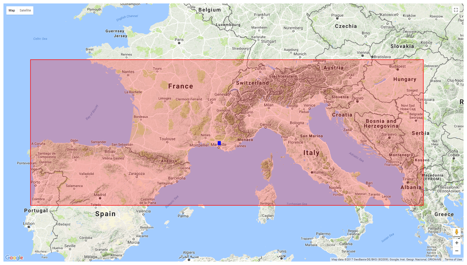
Figure 1Area defined for coincident measurements 40∘ N, 9∘ E to 48∘ N, 21∘ E. L'Observatoire de Haute Provence in blue at 43.93∘ N, 5.71∘ E (data: Google Maps, 2017).
For this study we wanted to compare temperature profiles measured from two different satellites in the region geographically near the lidar to minimize latitudinal variations in the temperature and within a small time frame to minimize the contribution of tides, tidal harmonics, and gravity wave effects. This desire for close spatio-temporal matching was balanced against the need for a sufficiently large number of comparisons as to produce results which are statistically significant and useful. Ultimately, we decided on a geographic window of ±4∘ latitude and ±15∘ longitude similar to the analysis done by Dou et al. (2009). We reasoned that the UMLT structure would vary with latitude to a greater degree than with longitude and that the longitudinal separation between consecutive SABER satellite passes gives a natural bound on the longitude. The contemporaneous work by Dawkins et al. (2018) includes a sensitivity study on the choice of longitudinal co-location limits. Their final choice for a spatial coincidence (±5∘ latitude, ±15∘ longitude) is comparable to our study which employs ±4∘ latitude, ±15∘ longitude. Figure 1 shows the geographic extent of our study.
The minimum length of an OHP nightly lidar temperature measurement is 4 h. We chose to use a ±4 h window around the lidar measurement as the temporal limit for coincidence with a satellite pass. This gives us a roughly 12 h window centred around the middle of the lidar measurement. Our choice was influenced by a desire to minimize the effect of the 12 h tidal harmonic. Authors of previous work making comparisons between satellites were able to take advantage of daytime satellite overpasses and chose to work within a ±2 h window (Hoppel et al., 2008). French and Mulligan (2010) conducted a comparison between an OH spectrometer (in conjunction with a sodium lidar) and SABER at ±15 min and ±8 h and found no significant difference. However, it must be noted that this study was conducted at a latitude of 69∘ S and the comparison may not hold in the mid-latitudes.
Here we demonstrate the directly calculated temperature biases between OHP and both SABER and MLS, which are present before we carry out the adjustment for satellite altitude offsets which are discussed in Sect. 5. An example of all three temperature profiles for the night of the 25 July 2012 is shown in Fig. 2. In this comparison the lidar profile was produced over 4 h and has a vertical resolution of 150 m from 30 to above 90 km. The large temperature uncertainty above 70 km is a result of the fine vertical resolution required to capture the mesospheric inversion layer present near 77 km.
4.1 Comparison OHP lidar and SABER
From 2002 to 2018 there were 1100 coincident measurements of sufficient quality between OHP lidars and SABER. Figure 3a shows the monthly median temperature differences between the lidar and SABER, while Fig. 3b shows the mean seasonal temperature bias with altitude.
Figure 3a contains the monthly median temperature differences between an OHP lidar temperature profile and a SABER temperature profile. After 2010 there are several time periods during which the Lidar Température et Aérosol (LTA) was not in routine operation or was in the process of being upgraded. To fill in these data gaps we have used temperature profiles derived from the ozone differential absorption lidar (DIAL), also referred to as Lidar Ozone Stratosphérique (LiO3S), which is described and validated for temperature in Wing et al. (2018). Given that the main scientific interest of LiO3S is stratospheric ozone, the noise floor of the raw lidar signal occurs at a lower altitude than for LTA for similar vertical integration. To produce temperature profiles which extend into the mesosphere, we use a coarser vertical resolution and a minimum altitude of 30 km, and often stop the temperature profile below 80 km if the temperature error becomes excessive.

Figure 2Example of co-located temperature profiles from the OHP lidar (green), SABER (blue), MLS (red), and MSIS (black).
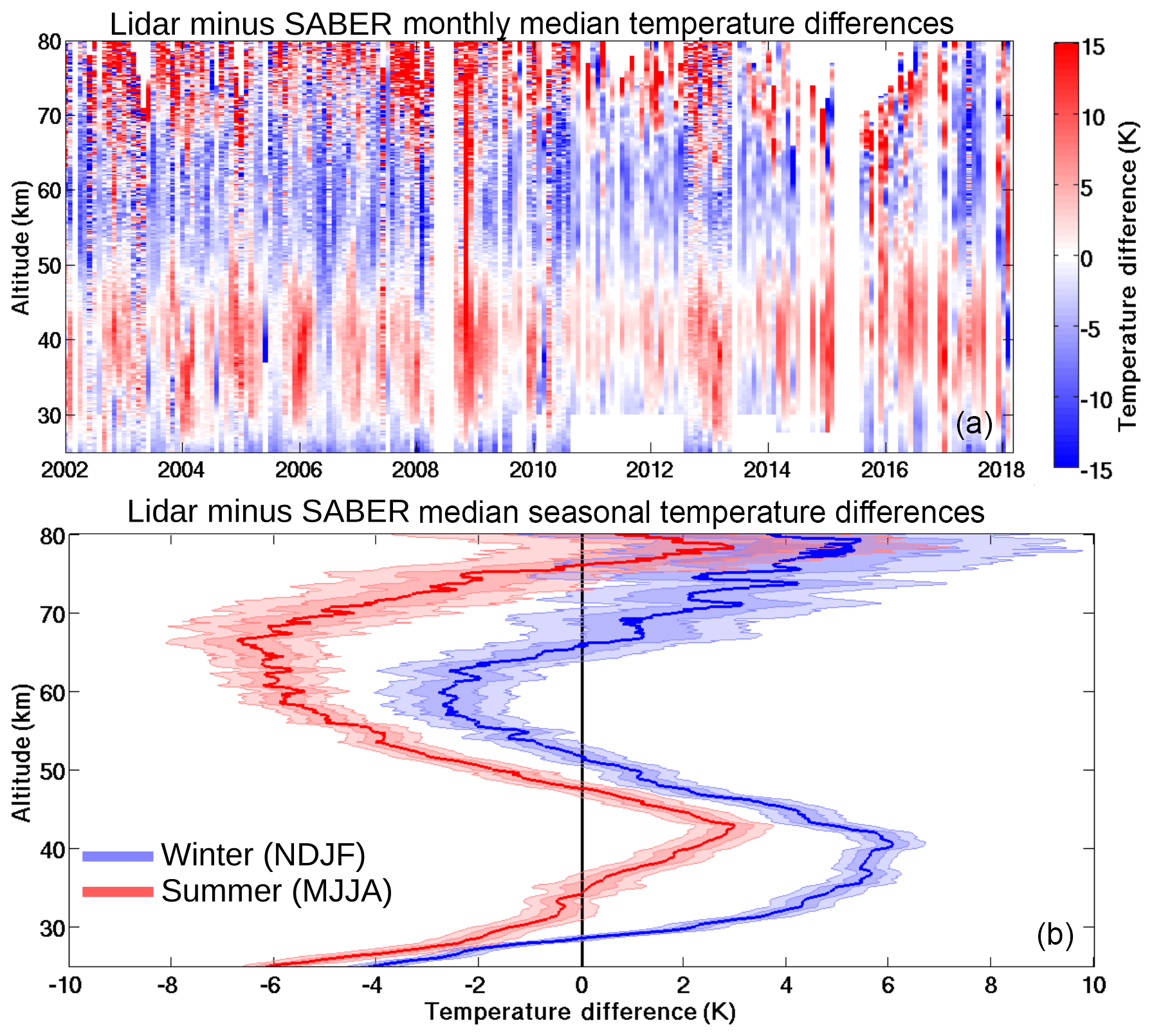
Figure 3The 16-year systematic comparison of OHP lidars and SABER temperatures. The monthly median temperature differences between the lidar and SABER are shown in panel (a). Red indicates that the lidar is warmer than SABER and blue that the lidar is colder. There are 1100 nights of coincident measurements in the colour plot. Panel (b) is a seasonal ensemble of lidar minus SABER temperature differences. The summer (May, June, July, August) ensemble in red includes 306 nights of coincident measurements, and the winter (November, December, January, February) ensemble in blue includes 397 nights of coincident measurements. Shaded errors represent 1 and 2 standard deviations.
Figure 3a shows a relative warm bias for the lidars with respect to SABER above 70 km. Discrepancies in this region are likely due to lidar initialization errors and background uncertainty, which we have attempted to minimize in the companion publication (Wing et al., 2018). There is also an evident seasonal relative warm bias in the winter stratosphere between 30 and 50 km – a region where lidar uncertainties in both altitude and temperature are well described (Leblanc et al., 2016a, b). Figure 3b shows a very distinctive “S” shape of the bias in both the winter and summer ensembles, which is indicative of a vertical offset between the lidar and satellite measurements. The basic S-shaped bias was identified in studies of synthetic lidar data as being due to vertical offsets between lidar instruments (Leblanc et al., 1998). Unfortunately, this offset is neither constant from night to night, nor constant with altitude, as evidenced by the elongated and distorted nature of the S shape.
If we bin all the temperature differences by month we can clearly see that there is a winter stratospheric warm bias below 45 km and a pronounced summer cold bias in the mesosphere between 50 and 70 km, as shown in Fig. 4.
4.2 Comparison OHP lidar and MLS
From 2004 to 2018 there were 1741 coincident measurements of sufficient quality between OHP lidars and MLS. Figure 5a shows the monthly median temperature differences between the lidar and MLS, while Fig. 5b shows the mean seasonal temperature bias with altitude.
As was the case with the lidar–SABER comparison, in Fig. 5a, we see a lidar warm bias above 70 km and a strong winter stratospheric warm bias near 45 km. In this comparison the stratospheric warm bias appears to have a downward phase migration as the winter progresses. In the corresponding panel, Fig. 5b, we see very pronounced summer time systematic differences which alternate from warm to cold throughout the stratosphere and mesosphere. The winter ensemble shows a very large lidar warm bias near the stratopause.
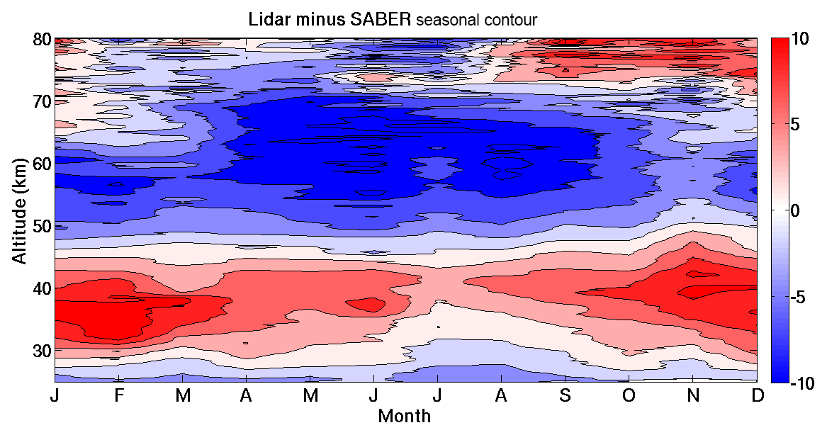
Figure 4Monthly median temperature difference between lidar and SABER temperature measurements. Red indicates regions where the lidar measures warmer temperatures than SABER and blue regions where the lidar measures colder temperatures than SABER.
Following the same procedure of binning lidar–MLS temperature differences by month, we see a very pronounced downward phase progression of the winter stratospheric warm bias from 45 km in January descending down to 40 km in February and March. Additionally, there is an evident layered cold bias in the summer stratosphere and mesosphere. The three layers appear near 37, 53, and 68 km in Fig. 6.
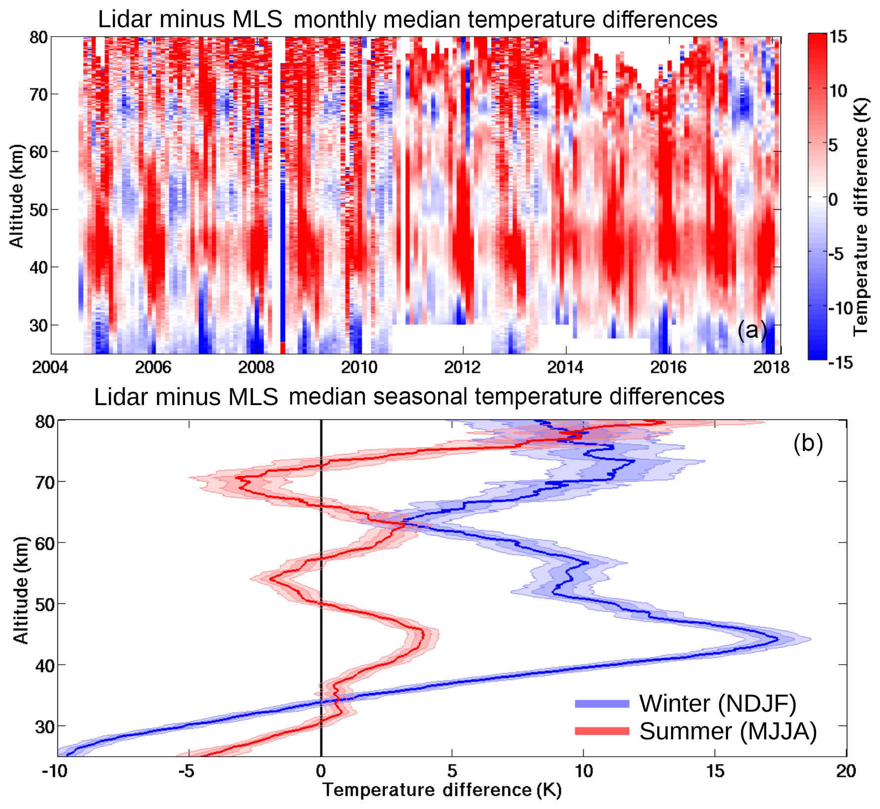
Figure 5The 14-year systematic comparison of OHP lidars and MLS temperatures. The monthly median temperature differences between the lidars and MLS are shown in panel (a). There are 1741 nights of coincident measurements. Panel (b) is a seasonal ensemble of lidar minus MLS temperature differences. The summer (May, June, July, August) ensemble in red includes 554 nights of coincident measurements and the winter (November, December, January, February) ensemble in blue includes 653 nights of coincident measurements. Shaded errors represent 1 and 2 standard deviations.
We investigated a possible vertical offset between the lidar and satellite measurements to determine whether this could be contributing to the temperature biases seen in Sect. 4.
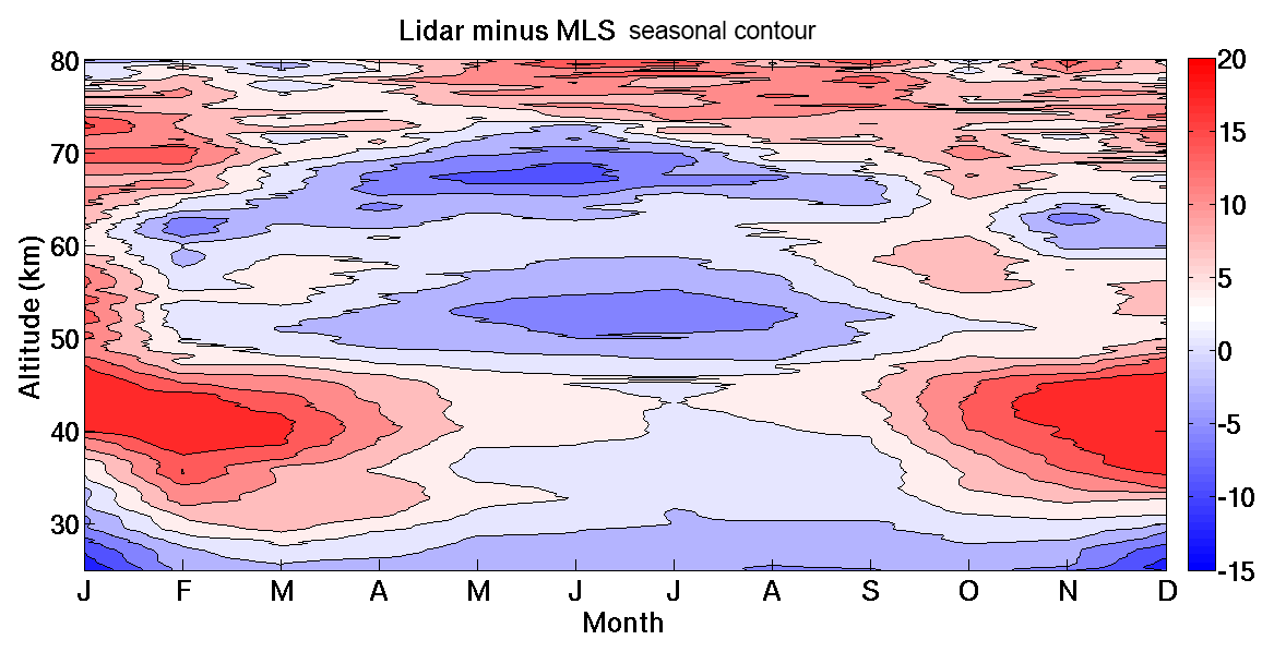
Figure 6Monthly median temperature difference between lidar and MLS temperature measurements. Red indicates regions where the lidar measures warmer temperatures than MLS and blue regions where the lidar measures colder temperatures than MLS.
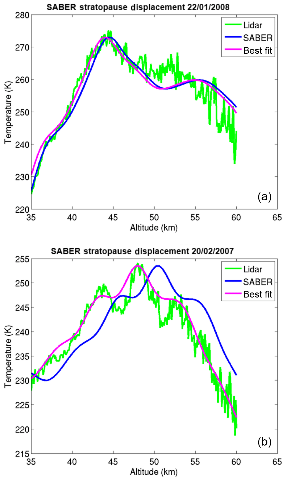
Figure 7Panel (a) shows a case in which the lidar and SABER were well aligned in altitude. Panel (b) shows a case in which a vertical displacement of the SABER profile ameliorated the agreement with the lidar measurement.
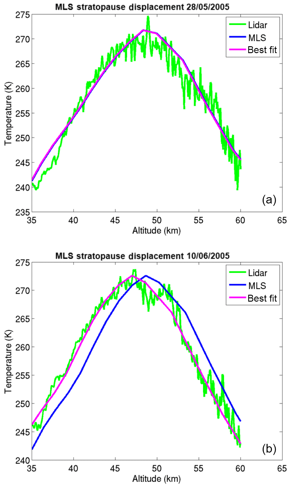
Figure 8Panel (a) shows a case in which the lidar and MLS were well aligned in altitude. Panel (b) shows a case in which a vertical displacement of the MLS profile ameliorated the agreement with the lidar measurement.
5.1 Method to determine the vertical offset between measurements
Matching the two temperature profiles exactly in amplitude and altitude requires a unique altitude-dependent correction factor for each comparison. However, we can make a rough estimate of the average vertical offset between the two measurements by focusing on the region of the stratopause which generally has a defined altitude and a clear structure. We used a simple least-squares method to best estimate the vertical offset that would minimize the temperature differences between the lidar measurement and the satellite measurement. Two examples of this offset calculation for SABER are shown in Fig. 7 and two examples for MLS are shown in Fig. 8. The examples in these figures show nights during which the lidar and satellite temperatures are in good agreement or can be brought into good agreement by applying a small vertical displacement. However, it is important to note that there are examples of lidar–satellite temperature measurements which cannot be brought into good agreement with small vertical displacements. Two such examples can be found in Fig. 9. These examples of poor agreement are almost exclusively found in winter on nights during which the stratopause is greatly disturbed.
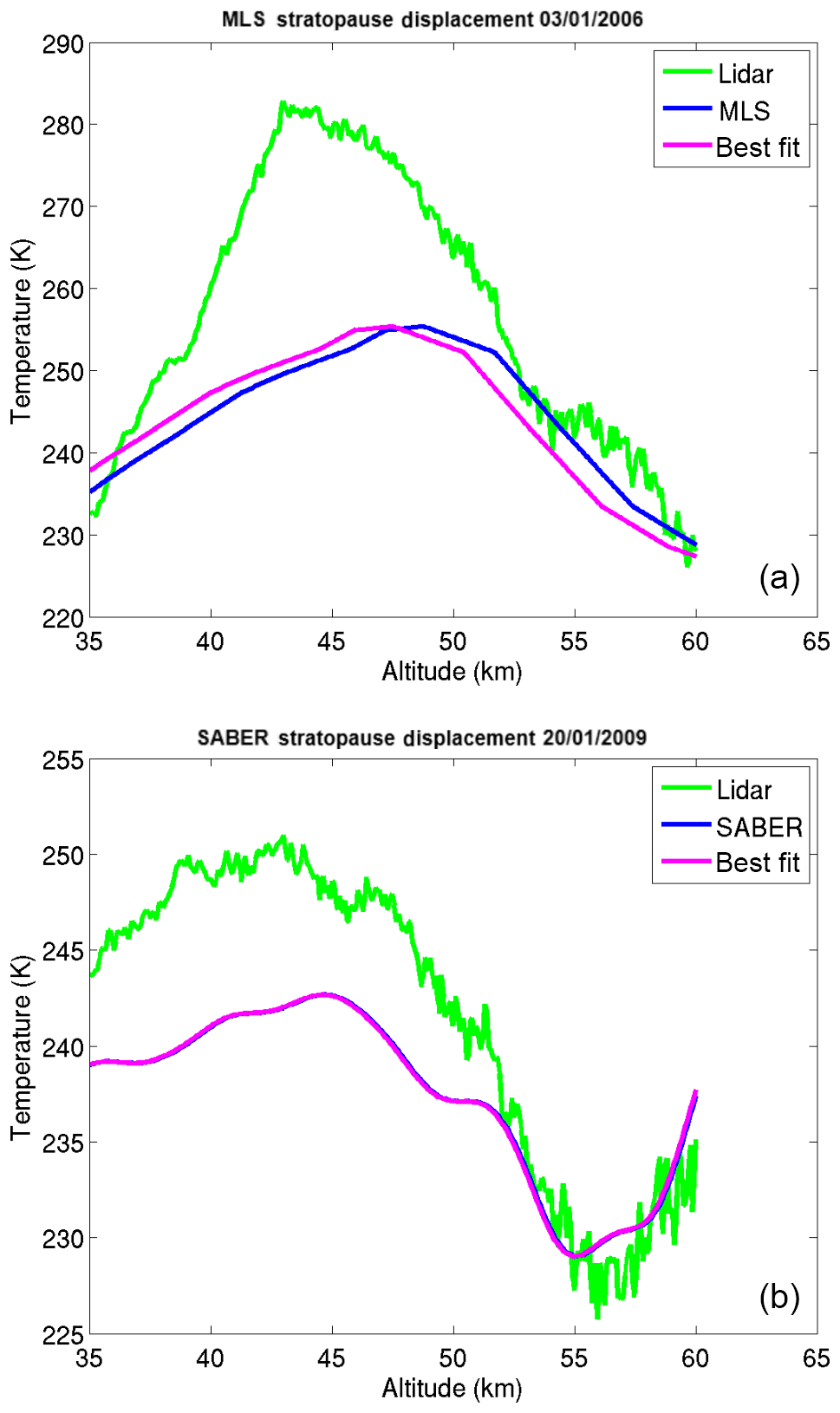
Figure 9Two examples of poor matches between lidar and satellite temperature profiles (MLS, a; SABER, b). These mismatches mainly occur between late November and early April on nights during which the stratosphere was disturbed and experiencing a warming.
5.2 Trends in vertical offset between lidar and satellites
We calculated an offset for every coincident measurement between the lidars and SABER and the lidars and MLS. The monthly average of this altitude offset value is represented in Fig. 10 as a green line for years during which the comparisons were primarily between LTA and the satellites and as a blue line for years during which LiO3S temperatures were used. The green and blue shaded regions are the respective standard deviations. Given the reduced vertical resolution of the temperature profiles from LiO3S, the least-squares minimized correction for stratopause height is less sensitive to small- and medium-scale fluctuations in the temperature profiles, such as the triple peak structure seen in Fig. 7b. As a result, comparisons between LiO3S and both satellites (blue curve in Fig. 10) tend toward the mean altitude displacement. This effect is more pronounced when comparing with SABER, which has a finer vertical resolution, than when comparing with MLS which has a coarser vertical resolution. There is a clear, but imperfect, seasonality to these altitude displacements.
Superimposing the traces shown in Fig. 10 onto the colour plots in Figs. 3 and 5 shows a clear correlation between lidar–satellite temperature anomalies and mean monthly altitude displacement between the lidar and satellite temperature profiles, as shown in Fig. 11.

Figure 10Panel (a) features the monthly average displacement of SABER measurements with respect to the OHP lidars (green for LTA and blue for LiO3S). The standard deviation is given as the shaded area. The mean offset (magenta) is 1446 m with a standard error of 49 m. Panel (b) shows the same analysis with the monthly average MLS displacement. The mean value is 911 m with a standard error of 90 m.
We have attempted to make a more accurate comparison of the lidar and satellite temperatures by using the stratopause height as a common altitude reference. We recalculated the lidar–satellite temperature differences shown in Figs. 4 and 6 after displacing the satellite measurement by a scalar value. Each satellite measurement was shifted vertically according to the lidar-derived stratospheric displacements shown in Fig. 10.
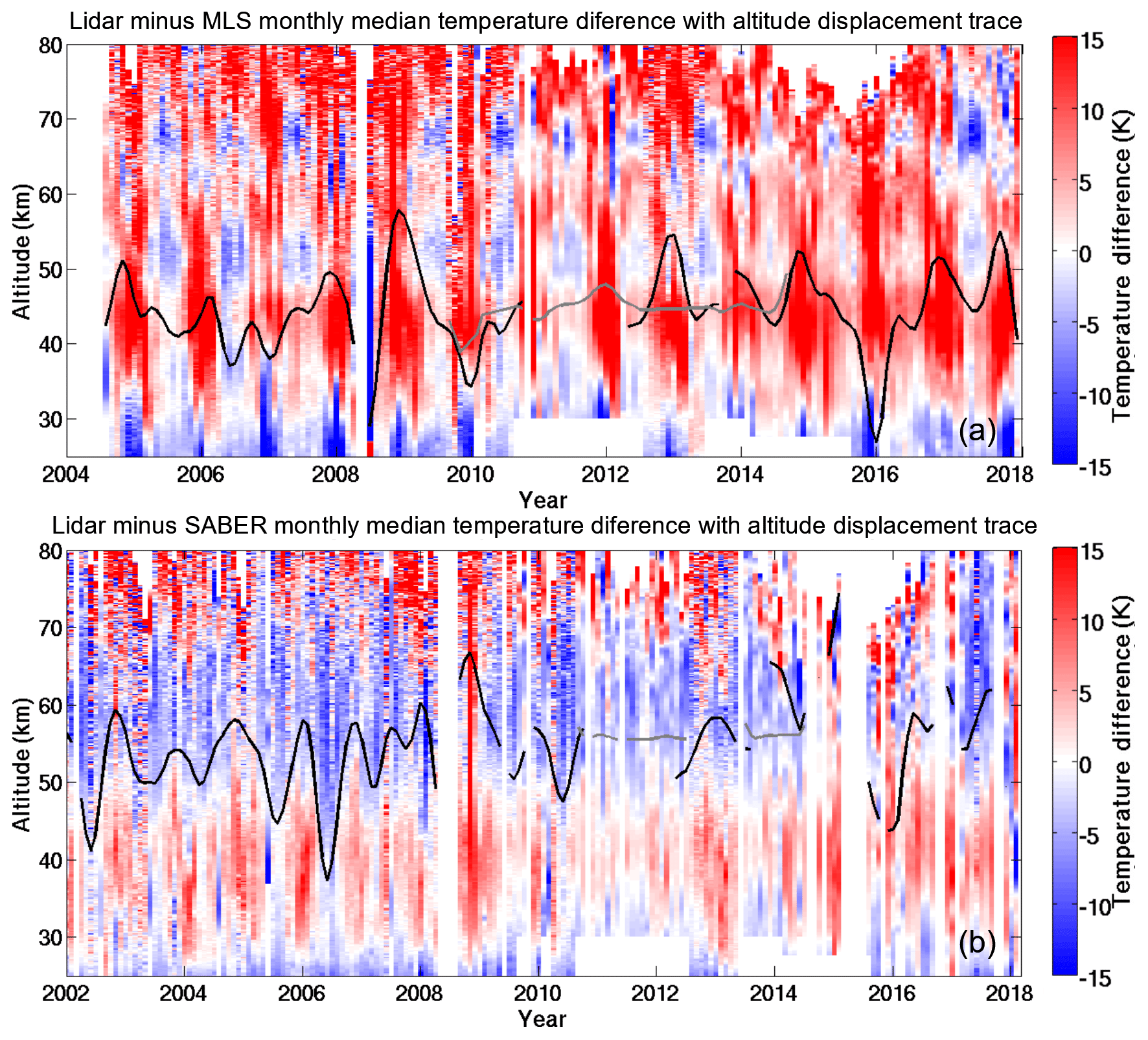
Figure 11Panel (a) features the monthly median temperature differences between the lidar and MLS seen in Fig. 5, with the estimated vertical displacement of the stratopause height overlaid. Panel (b) features the monthly median temperature differences between the lidar and SABER seen in Fig. 3, with the estimated vertical displacement of the stratopause height overlaid. The black line represents comparisons between LTA and the satellite, and the grey line represents comparisons between LiO3S and the satellite.
In Fig. 12 we see that by displacing the SABER temperature profiles so that the stratopause height is the same in both the lidar and satellite measurements we have reduced the maximum wintertime stratospheric warm bias from approximately 8 to 4 K. The summer time mesospheric cold bias of −10 K has likewise been reduced by between 4 and 6 K depending on altitude and season. The remaining bias in both the stratosphere and mesosphere cannot be further minimized by a simple vertical shift. The altitude-dependent correction which would be required to correct the temperature lapse rate is beyond the scope of this work.
In Fig. 13 we see that displacing the MLS temperature profiles was less successful than in the case of the SABER measurements. We have reduced the magnitude of beginning and end of wintertime stratospheric warm bias by up to 5 K during the months of March, April, October, and November, but the correction does not completely eliminate the issue. Additionally, we have an improvement of 5 K in the biased layer at 65 km. However, the horizontal layering inherent in the MLS temperature data makes determining a scalar correction even more challenging than in the case of SABER.
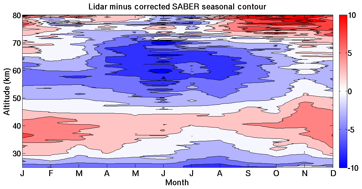
Figure 12Corrected seasonal temperature differences between the lidar and the vertically displaced SABER temperatures. The magnitude of the temperature differences is reduced in both the stratosphere and mesosphere over the majority of the altitude range when compared to a similar uncorrected temperature difference contour seen in Fig. 4.
We have replotted the seasonal ensemble temperature difference curves shown in Figs. 3b (lidar–SABER) and 5b (lidar–MLS) alongside the ensemble temperature differences after we applied the correction for stratopause height. Figure 14a shows the ensemble temperature difference for all 1741 lidar–MLS temperature comparisons before correction (red) and after correction (magenta). The prominent warm bias near 45 km has been reduced from 8 to 6 K but the cold biases at 53, and 68 km are made worse by the correction. To understand this result we can look at the seasonal dependence of the applied correction. Figure 14c is the summer ensemble temperature difference (MJJA) consisting of 554 lidar–MLS temperature comparisons before correction (red) and after correction (magenta). There is marginal improvement after correction below 55 km, but the change is not significant at 2σ and the structure of the temperature bias remains unchanged. Figure 14e is the winter ensemble temperature difference (NDJF) consisting of 653 lidar–MLS temperature comparisons before correction (blue) and after correction (magenta). There is significant improvement of 4 K in the large cold bias at 45 km. The corrected lidar–MLS comparison is also significantly worse near the cold bias at 63 km.

Figure 13Corrected seasonal temperature differences between the lidar and the vertically displaced MLS temperatures. The structured nature of the temperature bias seen in Fig. 6 remains unchanged by the vertical correction.
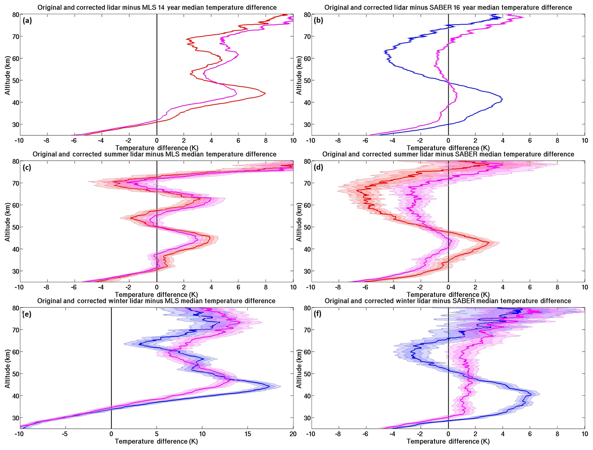
Figure 14Ensemble for lidar minus MLS temperature differences are in the left column (a, c, e) and lidar minus SABER are in the right column (b, d, f). Ensembles for all profiles are in the top row (a, b), summer (MJJA) profiles in the middle row (c, d), and winter (NDJF) in the bottom row (e, f). The uncorrected ensembles are in red and blue, and the ensembles after correction of the satellite stratopause altitude are in magenta. Panel (a) shows the median temperature difference for 1741 lidar minus MLS temperature profiles from 2004 to 2018, panel (c) shows the 554 lidar–MLS comparisons occurring during the summer (MJJ), and panel (e) shows the 653 lidar–MLS comparisons occurring during the winter (NDJF). Panel (b) shows the median temperature profiles from 2002 to 2018, panel (d) shows the 306 lidar–SABER comparisons occurring during the summer (MJJA), and panel (f) shows the 397 lidar–SABER comparisons occurring during the winter (NDJF).
Figure 14b shows the ensemble temperature difference for all 1100 lidar–SABER temperature comparisons before correction (blue) and after correction (magenta). The stratopause height correction has reduced the stratospheric warm bias from 4 K to less than 1 K and has reduced the mesospheric cold bias from −4 to −1 K. The warm bias above 70 km has been slightly increased. Figure 14d is the summer ensemble temperature difference (MJJA) consisting of 306 lidar–SABER temperature comparisons before correction (red) and after correction (magenta). There is a significant 3 K reduction in the warm bias at 45 km and a significant reduction in the mesospheric cold bias from −6 to −3 K. Figure 14f is the winter ensemble temperature difference (NDJF) consisting of 397 lidar–SABER temperature comparisons before correction (blue) and after correction (magenta). By applying the altitude correction we have eliminated the S shape in the temperature difference curve between 30 and 60 km. There is a significant 1 K constant warm bias that remains after correction. Above 70 km there is no statistically significant change.
7.1 The need for vertical altitude correction of satellite data
Improved observations of stratospheric and mesospheric temperature profiles and dynamical phenomena are required to advance our understanding of the middle atmosphere. The process of ground to satellite measurement comparison and validation is a vital ongoing scientific activity. By comparing long-term, stable, continuous, high-quality temperature measurements, such as those made by the lidars at OHP, to other data sets we can help to identify potential issues with calibration or retrieval algorithms.
We have presented individual cases in Figs. 7 and 8 in which both MLS and SABER temperature profiles benefited from a slight vertical displacement based on lidar-derived stratopause height. While this scalar adjustment does not correct for non-linear distortions in the altitude vector, it can significantly reduce the magnitude of the temperature bias in the stratosphere and lower mesosphere, as seen in Fig. 14a and b. This technique does not seem to work well when the stratopause is highly disturbed, as can be seen in the two wintertime examples in Fig. 9. The implications of satellite underestimation of sudden stratospheric warming events is of particular concern for reanalysis projects attempting to model middle atmosphere dynamics. However, using lidar data to supplement the satellite record, these fast dynamical processes can be better resolved.
An additional point about vertical resolutions should be made before further interpreting the results of our lidar–satellite temperature comparison. As was noted in Sect. 2 both MLS and SABER measure radiances on a pressure grid with reported vertical averaging kernels, whereas the lidar measures temperature on a fixed geometric altitude grid. SABER has a relatively small and uniform vertical resolution with a FWHM of 2 km, and MLS has a somewhat lower vertical resolution in the middle atmosphere, which increases with height, reaching a FWHM of 15 km at the top of our comparison region at 80 km. To make a fair comparison we have reduced the lidar vertical resolution to accommodate the satellites. There are considerations to keep in mind when comparing the results of the lidar–SABER and lidar–MLS temperature biases. The first is the effect that vertical resolution has on the temperature difference profile. SABER has a smaller FWHM and is therefore much more likely to reproduce the small-scale variations seen in the lidar data. This means that sharp features like the stratopause can easily be used as a tool for detecting possible bias. In contrast, MLS has a much wider FWHM, which means that we expect much less vertical fidelity in the lidar comparison. The lower vertical resolution should act to smooth out the temperature peaks and valleys in a way that may not correspond to the higher resolution ground-based measurements.
7.2 Temperature biases between OHP lidar and SABER
In the companion publication (Wing et al., 2018) we attempted to reduce the magnitude of the initialization-induced lidar warm bias, which is often reported above 70 km. We have reduced the bias by up to 5 K near 85 km and nearly 20 K at 90 km. Some residual systematic warm bias still remains between the lidar satellite comparisons in this publication.
The average 9.9±9.7 K bias at 80 km reported by Dawkins et al. (2018) using nine different metal layer resonance lidars compares favourably to our ensemble bias of 5 K at 80 km Fig. 14b. Given that the resonance lidars do not initialize their temperatures using the same inversion algorithm as the Rayleigh lidars, and that the resonance lidars have a minimum uncertainty near 85 km, perhaps our Rayleigh temperatures are not as influenced by our choice of the a priori density as we initially thought. Further work needs to be done on the topic of initialization-related bias to fully address the effects of noise and a priori choice on high-altitude Rayleigh lidar retrievals. However, we are encouraged by our results and cannot discount the possibility that some of the remaining temperature difference is due to errors or bias in the satellite altitudes.
When considering the residual temperature differences between the OHP lidars and SABER after the altitude correction based on lidar-derived stratopause height, we can see that much of the seasonally varying bias in the stratosphere and mesosphere has been reduced. We are still left with a general summertime cold bias over most of the atmospheric column, except near 45 km, which now achieves a maximum of −4 K in the June mesosphere. We cannot explain this bias from the perspective of the lidar data as nothing in our range resolution changes, our data acquisition cadence and measurement duration are very similar (Wing et al., 2018), and we are well into the linear region of lidar count rates and are not influenced by our a priori or saturated count rates. It is possible that there could be a tidal contribution as summer time lidar measurements start a bit later than wintertime measurements due to a shorter astronomical night. However, given that our criteria for coincidence were chosen to minimize the effects of the first few tidal harmonics, this seems unlikely. It is also possible that there is a seasonally dependent bias in the choice of a priori estimates used in the satellite retrieval of the geopotential height, which could influence the satellite altitude vector.
The cold bias seen below 30 km is most likely due to possible contamination in the lidar data from aerosols and saturation in the low-gain Rayleigh channel. Current OHP lidar measurements use Raman scatter data to correct for these effects and produce temperature profiles down to 5 km. However, these Raman data are not available for the entire 2002 to 2018 analysis period so we have opted not to include them in this work.
7.3 Temperature biases between OHP lidar and MLS
As with the comparison between the lidar and SABER, the lidar and MLS comparison has a pronounced warm bias above 70 km, which is in keeping with previous studies. However, the magnitude and extent of this warm bias in MLS are much more pronounced than in the SABER comparison plot. Much of this difference is due to the reduced vertical resolution of MLS at these high altitudes. This holds true particularly when comparing lower vertical resolution lidar data to MLS.
The lidar MLS comparison has a wintertime stratospheric warm bias which is not much reduced by simply shifting the location of the MLS stratopause (Fig. 14e). We have reduced the magnitude of the difference by 4 K, but the stratopause altitude correction was markedly less successful than in the case with SABER. It is almost universally the case that sudden stratospheric warmings seen by the lidar are missed or smoothed over in the corresponding MLS measurement. Figure 9a is very much a typical comparison for periods when the stratosphere is highly disturbed. There is a limit to how much can be done to improve the lidar–MLS comparison using a simple scalar correction.
The vertical structure which dominates much of the middle portion of the lidar MLS comparison is also difficult to account for. The structure is particularly evident in Fig. 14c and is nearly insensitive to our applied altitude correction. There is nothing in the lidar technique that could explain this pattern. A similar horizontal banding pattern is seen in the comparison of MLS to the European Centre for Medium-range Weather Forecasts (ECMWF) assimilation in the MLS geopotential validation paper (Schwartz et al., 2008). The effect is most likely an artefact introduced in some stage of the satellite retrieval. Studies like ours provide a perfect opportunity to incorporate lidar information into the satellite retrieval and improve the satellite data products. Given the confidence we have in the fixed width and amplitude of the vertical kernels in the lidar measurement, a lidar altitude and temperature vector could be used to recalculate the MLS geopotential and temperature profiles to help identify the source of this artefact.
It is also important to acknowledge that simply correcting for stratopause height offset was counterproductive for our lidar–MLS comparisons above 50 km, as seen in Fig. 14a. It is likely that any potential lidar-derived correction for MLS will be more complex than a simple scalar offset. Such a correction may even have different functional forms in the stratosphere and mesosphere.
7.4 Comparison with previous work
We can compare our results to a few of the studies involving Rayleigh lidar cited in the Introduction; however, it is important to note a few caveats. The methodologies of the different studies vary significantly and a direct comparison between our work and previous studies is fraught with confounding variables, differences in sampling size, and statistics. As a brief reminder, our work was done in a 30∘ by 8∘ geographic box centred on the OHP and had a temporal coincidence window of 12 h. We then made nightly average temperature differences between the lidar and satellites and presented the monthly medians of those temperature differences over the span of each satellite (2002–present for SABER and 2004–present for MLS).
The two studies by Sivakumar (Sivakumar et al., 2011; Siva Kumar et al., 2003) made use of monthly averaged lidar and SABER temperatures and found semi-annual temperature anomalies of 3–5 K in the stratopause region during February–March and September–October, which was attributed to averaging and possibly the annual oscillation. We have shown a similar temperature difference in the stratopause of 4 K in the summer before altitude corrections, reduced to zero bias after altitude correction, and 6 K in the winter before altitude corrections, reduced to 1 K after altitude correction. We have correlated this temperature bias directly to a vertical displacement of the satellite altitude with respect to the lidar altitude and not to the annual oscillation. Further work must be done to explore the possibility of North Atlantic Oscillation or annual oscillation effects, but a quick correlation of relative vertical displacement is seen in Fig. 10 and a monthly average AO phase shows an R-squared value of only 0.04 for SABER and 0.03 for MLS. There are isolated periods of up to a year for which it seems like the correlations are significant; however, it is clear that over a period of nearly a decade, the AO phase and wintertime stratospheric temperature anomalies are not correlated.
The study by Yue et al. (2014) compared 120 nights of lidar temperatures to SABER monthly average temperatures and found wintertime temperature anomalies in the stratopause region of 5 K. The stratospheric warm bias was attributed to tides; however, this explanation cannot explain the seasonal nature of this bias found in this work, nor can it explain why a simple vertical displacement of the satellite stratopause height offers a suitable correction. Subsequent to this work, Hauchecorne et al. (2018) published a temperature data set derived from GOMOS stellar occultation measurements, which were validated using Rayleigh lidar. In this paper, the tidal contribution to the lidar–satellite temperature bias in the stratosphere is estimated to be less than 2 K, based on tidal characteristics extracted from the Global Scale Wave Model for tides.
The same 2–5 K stratopause temperature bias was found by Dou et al. (2009). This study used 2332 nights of lidar data from six different NDACC lidars and compared them with the zonal mean temperatures from SABER. The bias was attributed to possible tidal aliasing or aerosol contamination. In Part 1 of this paper we note that contamination by aerosols is not significant above 30 or 35 km and that aerosols cannot be responsible for lidar temperature bias in the stratopause. As was stated in the previous paragraph, Hauchecorne et al. (2018) estimate an upper limit on the effect of tidal aliasing for a small geographic area of less than 2 K. It is possible that tides could play a larger role when comparing measurements from a localized lidar ground site to a zonal average temperature from a satellite. The altitude corrections shown in the present paper account for all 4 K of temperature bias in summer and 5 of 6 K of bias during winter. This type of correction may account fully for the stratopause temperature bias reported by Dou et al. (2009).
In summary, previous studies have shown a consistent systematic temperature bias of 2 to 5 K between different independent lidars and SABER near the stratopause. Tides, aerosols, planetary oscillations, and satellite calibration errors were all given as possible sources of error when accounting for this discrepancy. Our study has shown that the temperature bias has a clear seasonality, with the largest temperature differences occurring in the winter months. We have also shown that a simple vertical correction of the satellite temperatures based on the height of the stratopause, as measured by the lidar, significantly reduces the bias.
We can draw the following conclusions from the comparison of the lidar and satellite temperature measurements.
-
We have found the same systematic 5–15 K warm bias in the lidar–satellite comparisons above 70 km found in studies like García-Comas et al. (2014), Taori et al. (2011, 2012a, b), Dou et al. (2009), Remsberg et al. (2008), Yue et al. (2014), Dawkins et al. (2018), and Sivakumar et al. (2011). We have attempted to carefully account for the background-induced warm bias in high-altitude Rayleigh lidar temperatures. We believe that the algorithm set out in the companion publication (Wing et al., 2018) is robust and accounts for many of the uncertainties in the lidar initialization process. However, we are as yet unable to determine to what extent the a priori estimate warms the lidar temperature retrieval at these heights.
-
We have seen a layered summer stratosphere–mesosphere cold bias in lidar–MLS seasonal temperature comparisons with peak differences at 37, 50, and 65 km. There is nothing in the lidar data or retrieval algorithm which could account for this structure. The results of this study will be useful for any future satellite validation studies in the style of Schwartz et al. (2008) for which lidar data could be used as a reference data set. In particular, lidar–satellite bias study results are useful for the ongoing NASA project “The Mesospheric and Upper Stratospheric Temperature and Related Datasets” (MUSTARD), which seeks to merge historic and ongoing satellite data sets.
-
The persistent summertime cold bias between the lidar and SABER results from a disagreement in the thermal lapse rate above and below the stratopause, which is independent of the scalar stratopause height offset. Given that lapse rate is a fundamental geophysical parameter further work, must be done to explore possible errors in vertical resolution and altitude definition.
-
The periods of greatest lidar–satellite temperature disagreement are found during times when the middle atmosphere is highly disturbed. In particular, the amplitude of stratospheric warming events can be underestimated and features like double stratopauses can be missed in the satellite measurements.
We have shown that ground-based lidars can provide reliable and consistent temperature measurements over decades. This kind of high vertical resolution temperature database is useful, both as a validation source for other instruments and for fundamental geophysical research.
The data used in this paper were obtained as part of the Network for the Detection of Atmospheric Composition Change (NDACC; see http://www.ndsc.ncep.noaa.gov/data/, last access: 17 December 2018), the SABER data centre (see http://saber.gats-inc.com/data.php, last access: 17 December 2018), and the MLS data centre (see https://mls.jpl.nasa.gov, last access: 17 December 2018) and are publicly available.
RW conceived of the presented idea, wrote the required codes, reprocessed the data, performed the computations, and wrote the manuscript. AH and PK supervised the work, provided access to LTA data, and offered scientific insight. SGB provided access to LiO3S data and offered scientific insight. SK helped supervise the work and offered scientific insight. EMM edited the drafts, provided key criticisms to improve the work, helped refine the ideas in the manuscript, and provided scientific insight. All authors discussed the results and contributed to the final paper.
The authors declare that they have no conflict of interest.
This work is supported by the project Atmospheric dynamics Research
InfraStructure Project (ARISE 2) funded by the European Union's
Horizon 2020 Research and Innovation programme under grant agreement no. 653980. French NDACC activities are supported by Institut National des
Sciences de l'Univers/Centre National de la Recherche Scientifique
(INSU/CNRS), Université de Versailles Saint-Quentin-en-Yvelines (UVSQ),
and Centre National d'Études Spatiales (CNES). The authors would also like
to thank the technicians at La Station Géophysique Gérard Mégie
at OHP.
Edited by: Markus Rapp
Reviewed by: two anonymous referees
Chu, X., Pan, W., Papen, G. C., Gardner, C. S., and Gelbwachs, J. A.: Fe Boltzmann Temperature Lidar: Design, Error Analysis, and Initial Results at the North and South Poles, Appl. Optics, 41, 4400–4410, https://doi.org/10.1364/AO.41.004400, 2002. a
Council, N. R.: Earth Science and Applications from Space: National Imperatives for the Next Decade and Beyond, The National Academies Press, Washington, DC, https://doi.org/10.17226/11820, available at: https://www.nap.edu/catalog/11820/earth-science-and-applications-from-space-national-imperatives-for-the (last access: 28 May 2018), 2007. a
Google Maps: Observatoire de Haute Provence (CNRS) Kernel Description, available at: https://www.google.fr/maps/place/Observatoire+de+Haute+Provence+(CNRS)/@43.9236737,5.7183398, last access: 30 November 2017. a
Dawkins, E. C. M., Feofilov, A., Rezac, L., Kutepov, A. A., Janches, D., Höffner, J., Chu, X., Lu, X., Mlynczak, M. G., and Russell, J.: Validation of SABER v2.0 Operational Temperature Data With Ground-Based Lidars in the Mesosphere-Lower Thermosphere Region (75–105 km), J. Geophys. Res.-Atmos., 123, 9916–9934, https://doi.org/10.1029/2018JD028742, 2018. a, b, c, d, e
Dou, X., Li, T., Xu, J., Liu, H.-L., Xue, X., Wang, S., Leblanc, T., McDermid, I. S., Hauchecorne, A., Keckhut, P., Bencherif, H., Heinselman, C., Steinbrecht, W., Mlynczak, M. G., and Russell, J. M.: Seasonal oscillations of middle atmosphere temperature observed by Rayleigh lidars and their comparisons with TIMED/SABER observations, J. Geophys. Res.-Atmos., 114, D20103, https://doi.org/10.1029/2008JD011654, 2009. a, b, c, d, e
French, W. J. R. and Mulligan, F. J.: Stability of temperatures from TIMED/SABER v1.07 (2002–2009) and Aura/MLS v2.2 (2004–2009) compared with OH(6–2) temperatures observed at Davis Station, Antarctica, Atmos. Chem. Phys., 10, 11439–11446, https://doi.org/10.5194/acp-10-11439-2010, 2010. a
García-Comas, M., Funke, B., Gardini, A., López-Puertas, M., Jurado-Navarro, A., von Clarmann, T., Stiller, G., Kiefer, M., Boone, C. D., Leblanc, T., Marshall, B. T., Schwartz, M. J., and Sheese, P. E.: MIPAS temperature from the stratosphere to the lower thermosphere: Comparison of vM21 with ACE-FTS, MLS, OSIRIS, SABER, SOFIE and lidar measurements, Atmos. Meas. Tech., 7, 3633–3651, https://doi.org/10.5194/amt-7-3633-2014, 2014. a, b
Hauchecorne, A., Blanot, L., Wing, R., Keckhut, P., Khaykin, S., Bertaux, J.-L., Meftah, M., Claud, C., and Sofieva, V.: A new MesosphEO dataset of temperature profiles from 35 to 85 km using Rayleigh scattering at limb from GOMOS/ENVISAT daytime observations, Atmos. Meas. Tech. Discuss., https://doi.org/10.5194/amt-2018-241, in review, 2018. a, b
Hoppel, K. W., Baker, N. L., Coy, L., Eckermann, S. D., McCormack, J. P., Nedoluha, G. E., and Siskind, D. E.: Assimilation of stratospheric and mesospheric temperatures from MLS and SABER into a global NWP model, Atmos. Chem. Phys., 8, 6103–6116, https://doi.org/10.5194/acp-8-6103-2008, 2008. a
Johnson, K. W. and Gelman, M. E.: Trends in upper stratospheric temperatures as observed by rocketsondes (1965–1983), International Council of Scientific Unions Handbook for MAP, International Council of Scientific Unions, Urbana, IL, USA, 18, 1985. a
Leblanc, T., McDermid, I. S., Hauchecorne, A., and Keckhut, P.: Evaluation of optimization of lidar temperature analysis algorithms using simulated data, J. Geophys. Res.-Atmos., 103, 6177–6187, https://doi.org/10.1029/97JD03494, 1998. a
Leblanc, T., Sica, R. J., van Gijsel, J. A. E., Godin-Beekmann, S., Haefele, A., Trickl, T., Payen, G., and Gabarrot, F.: Proposed standardized definitions for vertical resolution and uncertainty in the NDACC lidar ozone and temperature algorithms – Part 1: Vertical resolution, Atmos. Meas. Tech., 9, 4029–4049, https://doi.org/10.5194/amt-9-4029-2016, 2016a. a
Leblanc, T., Sica, R. J., van Gijsel, J. A. E., Haefele, A., Payen, G., and Liberti, G.: Proposed standardized definitions for vertical resolution and uncertainty in the NDACC lidar ozone and temperature algorithms – Part 3: Temperature uncertainty budget, Atmos. Meas. Tech., 9, 4079–4101, https://doi.org/10.5194/amt-9-4079-2016, 2016b. a
Licel: Licel Data Sheet Kernel Description, available at: https://http://licel.com/transdat.htm#DNL, last access: 8 August 2018. a
Livesey, N. J., Snyder, W. V., Read, W. G., and Wagner, P. A.: Retrieval algorithms for the EOS Microwave limb sounder (MLS), IEEE T. Geosci. Remote, 44, 1144–1155, https://doi.org/10.1109/TGRS.2006.872327, 2006. a
Meek, C. E., Manson, A. H., Hocking, W. K., and Drummond, J. R.: Eureka, 80∘ N, SKiYMET meteor radar temperatures compared with Aura MLS values, Ann. Geophys., 31, 1267–1277, https://doi.org/10.5194/angeo-31-1267-2013, 2013. a
Mertens, C. J., Mlynczak, M. G., López-Puertas, M., Wintersteiner, P. P., Picard, R. H., Winick, J. R., Gordley, L. L., and Russell, J. M.: Retrieval of mesospheric and lower thermospheric kinetic temperature from measurements of CO2 15 µm Earth Limb Emission under non-LTE conditions, Geophys. Res. Lett., 28, 1391–1394, https://doi.org/10.1029/2000GL012189, 2001. a, b
Pautet, P.-D., Taylor, M. J., Pendleton, W. R., Zhao, Y., Yuan, T., Esplin, R., and McLain, D.: Advanced mesospheric temperature mapper for high-latitude airglow studies, Appl. Optics, 53, 5934–5943, https://doi.org/10.1364/AO.53.005934, 2014. a
Remsberg, E. E., Marshall, B. T., Garcia-Comas, M., Krueger, D., Lingenfelser, G. S., Martin-Torres, J., Mlynczak, M. G., Russell, J. M., Smith, A. K., Zhao, Y., Brown, C., Gordley, L. L., Lopez-Gonzalez, M. J., Lopez-Puertas, M., She, C.-Y., Taylor, M. J., and Thompson, R. E.: Assessment of the quality of the Version 1.07 temperature-versus-pressure profiles of the middle atmosphere from TIMED/SABER, J. Geophys. Res.-Atmos., 113, D17101, https://doi.org/10.1029/2008JD010013, 2008. a, b
Schwartz, M. J., Lambert, A., Manney, G. L., Read, W. G., Livesey, N. J., Froidevaux, L., Ao, C. O., Bernath, P. F., Boone, C. D., Cofield, R. E., Daffer, W. H., Drouin, B. J., Fetzer, E. J., Fuller, R. A., Jarnot, R. F., Jiang, J. H., Jiang, Y. B., Knosp, B. W., Krüger, K., Li, J. F., Mlynczak, M. G., Pawson, S., Russell, J. M., Santee, M. L., Snyder, W. V., Stek, P. C., Thurstans, R. P., Tompkins, A. M., Wagner, P. A., Walker, K. A., Waters, J. W., and Wu, D. L.: Validation of the Aura Microwave Limb Sounder temperature and geopotential height measurements, J. Geophys. Res.-Atmos., 113, D15S11, https://doi.org/10.1029/2007JD008783, 2008. a, b, c, d
Siva Kumar, V., Rao, P. B., and Krishnaiah, M.: Lidar measurements of stratosphere-mesosphere thermal structure at a low latitude: Comparison with satellite data and models, J. Geophys. Res.-Atmos., 108, 4342, https://doi.org/10.1029/2002JD003029, 2003. a, b
Sivakumar, V., Vishnu Prasanth, P., Kishore, P., Bencherif, H., and Keckhut, P.: Rayleigh LIDAR and satellite (HALOE, SABER, CHAMP and COSMIC) measurements of stratosphere-mesosphere temperature over a southern sub-tropical site, Reunion (20.8∘ S; 55.5∘ E): climatology and comparison study, Ann. Geophys., 29, 649–662, https://doi.org/10.5194/angeo-29-649-2011, 2011. a, b, c
Taori, A., Dashora, N., Raghunath, K., Russell, J. M., and Mlynczak, M. G.: Simultaneous mesosphere-thermosphere-ionosphere parameter measurements over Gadanki (13.5∘ N, 79.2∘ E): First results, J. Geophys. Res.-Space, 116, A07308, https://doi.org/10.1029/2010JA016154, 2011. a, b
Taori, A., Jayaraman, A., Raghunath, K., and Kamalakar, V.: A new method to derive middle atmospheric temperature profiles using a combination of Rayleigh lidar and O2 airglow temperatures measurements, Ann. Geophys., 30, 27–32, https://doi.org/10.5194/angeo-30-27-2012, 2012a. a, b
Taori, A., Kamalakar, V., Raghunath, K., Rao, S., and Russell, J.: Simultaneous Rayleigh lidar and airglow measurements of middle atmospheric waves over low latitudes in India, J. Atmos. Sol.-Terr., 78–79, 62–69, https://doi.org/10.1016/j.jastp.2011.06.012, 2012b. a, b
Waters, J. W., Froidevaux, L., Harwood, R. S., Jarnot, R. F., Pickett, H. M., Read, W. G., Siegel, P. H., Cofield, R. E., Filipiak, M. J., Flower, D. A., Holden, J. R., Lau, G. K., Livesey, N. J., Manney, G. L., Pumphrey, H. C., Santee, M. L., Wu, D. L., Cuddy, D. T., Lay, R. R., Loo, M. S., Perun, V. S., Schwartz, M. J., Stek, P. C., Thurstans, R. P., Boyles, M. A., Chandra, K. M., Chavez, M. C., Chen, G.-S., Chudasama, B. V., Dodge, R., Fuller, R. A., Girard, M. A., Jiang, J. H., Jiang, Y., Knosp, B. W., LaBelle, R. C., Lam, J. C., Lee, K. A., Miller, D., Oswald, J. E., Patel, N. C., Pukala, D. M., Quintero, O., Scaff, D. M., Snyder, W. V., Tope, M. C., Wagner, P. A., and Walch, M. J.: The Earth observing system microwave limb sounder (EOS MLS) on the aura Satellite, IEEE T. Geosci. Remote, 44, 1075–1092, https://doi.org/10.1109/TGRS.2006.873771, 2006. a, b
Wing, R., Hauchecorne, A., Keckhut, P., Godin-Beekmann, S., Khaykin, S., McCullough, E. M., Mariscal, J.-F., and d'Almeida, É.: Lidar temperature series in the middle atmosphere as a reference data set – Part 1: Improved retrievals and a 20-year cross-validation of two co-located French lidars, Atmos. Meas. Tech., 11, 5531–5547, https://doi.org/10.5194/amt-11-5531-2018, 2018. a, b, c, d, e, f, g
Wuebbles, D., Fahey, D., and Hibbard, K.: The Climate Science Special Report (CSSR) of the Fourth National Climate Assessment (NCA4), in: AGU Fall Meeting Abstracts, 12–16 December 2016, San Francisco, CA, USA, 2016. a
Xu, J., She, C. Y., Yuan, W., Mertens, C., Mlynczak, M., and Russell, J.: Comparison between the temperature measurements by TIMED/SABER and lidar in the midlatitude, J. Geophys. Res.-Space, 111, A10S09, https://doi.org/10.1029/2005JA011439, 2006. a
Yuan, T., She, C.-Y., Krueger, D., Reising, S. C., Zhang, X., and Forbes, J.: A collaborative study on temperature diurnal tide in the midlatitude mesopause region (41∘ N, 105∘ W) with Na lidar and TIMED/SABER observations, J. Atmos. Sol.-Terr., 72, 541–549, https://doi.org/10.1016/j.jastp.2010.02.007, 2010. a
Yue, C., Yang, G., Wang, J., Guan, S., Du, L., Cheng, X., and Yang, Y.: Lidar observations of the middle atmospheric thermal structure over north China and comparisons with TIMED/SABER, J. Atmos. Sol.-Terr., 120, 80–87, https://doi.org/10.1016/j.jastp.2014.08.017, 2014. a, b, c, d, e
- Abstract
- Introduction
- Instrumentation
- Comparison parameters
- Temperature comparisons without considering vertical offset
- Minimizing temperature difference between lidar and satellites with a vertical offset
- Recalculated lidar–satellite temperature differences
- Discussion
- Conclusions
- Data availability
- Author contributions
- Competing interests
- Acknowledgements
- References