the Creative Commons Attribution 3.0 License.
the Creative Commons Attribution 3.0 License.
Intercalibration between HIRS/2 and HIRS/3 channel 12 based on physical considerations
Kostas Eleftheratos
Robert Sausen
High-resolution Infrared Radiation Sounder (HIRS) brightness temperatures at channel 12 (T12) can be used to assess the water vapour content of the upper troposphere. The transition from HIRS/2 to HIRS/3 in 1999 involved a shift in the central wavelength of channel 12 from 6.7 to 6.5 µm, causing a discontinuity in the time series of T12. To understand the impact of this change in the measured brightness temperatures, we have performed radiative transfer calculations for channel 12 of HIRS/2 and HIRS/3 instruments, using a large set of radiosonde profiles of temperature and relative humidity from three different sites. Other possible changes within the instrument, apart from the changed spectral response function, have been assumed to be of minor importance, and in fact, it was necessary to assume as a working hypothesis that the spectral and radiometric calibration of the two instruments did not change during the relatively short period of their common operation. For each radiosonde profile we performed two radiative transfer calculations, one using the HIRS/2 channel response function of NOAA 14 and one using the HIRS/3 channel response function of NOAA 15, resulting in negative differences of T12 (denoted as ) ranging between −12 and −2 K. Inspection of individual profiles for large, medium and small values of ΔT12 pointed to the role of the mid-tropospheric humidity. This guided us to investigate the relation between ΔT12 and the channel 11 brightness temperatures which are typically used to detect signals from the mid-troposphere. This allowed us to construct a correction for the HIRS/3 T12, which leads to a pseudo-channel 12 brightness temperature as if a HIRS/2 instrument had measured it. By applying this correction we find an excellent agreement between the original HIRS/2 T12 and the HIRS/3 data inferred from the correction method with R=0.986. Upper-tropospheric humidity (UTH) derived from the pseudo HIRS/2 T12 data compared well with that calculated from intersatellite-calibrated data, providing independent justification for using the two intercalibrated time series (HIRS/2 and HIRS/3) as a continuous HIRS time series for long-term UTH analyses.
- Article
(1102 KB) -
Supplement
(245 KB) - BibTeX
- EndNote


Climate variability studies require the analysis of long homogeneous time series of climate data. For example, a long time series which can be used to study the variability of upper-tropospheric water vapour can be derived from the brightness temperature measurements of the High-resolution Infrared Radiation Sounder (HIRS) instrument aboard the National Oceanic and Atmospheric Administration (NOAA) polar orbiting satellites. The HIRS measurements started in mid-1979 and are still ongoing. They provide a unique long-term data set (covering nearly 4 decades) that can be exploited in climate research. When NOAA launched the weather satellite NOAA 15 in 1998, it was equipped similarly to all its precursors with a HIRS instrument. This 20-channel instrument provides information on temperature and humidity in the troposphere, where channels 10 to 12 are sensitive to water vapour at different altitude bands (lower to upper troposphere, Soden and Bretherton, 1996). Unfortunately, with the launch of NOAA 15 the central frequency in channel 12 has moved from 6.7 to 6.5 µm. This is quite a large change, because it means that the channel has its maximum sensitivity about 1 km higher (and accordingly several degrees colder) than channel 12 of all previous satellites.
With that change, i.e. the transition from HIRS/2 on the older NOAA satellites to HIRS/3 on NOAA 15, the channel 12 time series became inhomogeneous. Shi and Bates (2011) performed an intercalibration based on statistics of differences between the brightness temperatures measured by subsequent HIRS instruments (technically a regression of first kind). The intercalibration solved the problem of a broken time series for some of the statistics of the data, e.g. for the mean values. The intercalibrated time series was used for several studies (e.g. Gierens et al., 2014; Chung et al., 2016). Yet problems remained in the lower tail of the distribution of brightness temperatures, that is, at the lowest values of brightness temperatures, as has been detected by Gierens and Eleftheratos (2017, in the following cited as GE17).
However, the question arises as to whether it is sufficient to solve a physical problem (i.e. the different altitudes of peak sensitivity of the channel 12 on HIRS/2 and HIRS/3) with a purely statistical method. Hence, GE17 posed the following question.
“Is it justified at all to combine all HIRS T12 (the brightness temperature measured by channel 12) data into a single time series when it is a matter of fact that HIRS 2 and HIRS 3/4 sense different layers of the upper troposphere, layers that overlap heavily but whose centres are more than one kilometre apart vertically?”
In fact, this question can be broken down into sub-questions. (1) Under which circumstances is the Shi and Bates (2011) intercalibration justified or not? (2) Which assumptions have to be made about the structure of temperature and moisture profiles? The present paper deals with these questions. Fortunately it turns out that it is possible and justified to combine the channel 12 time series on physical reasoning providing a homogeneous time series of 35+ years that can be used for climatological studies. In this paper we demonstrate that independent tests based on results from radiative transfer calculations lead to a comparison between NOAA 14 and NOAA 15 channel 12 brightness temperatures that is very similar to the same comparison performed with the intercalibrated data from Shi and Bates (2011). For these tests we assume that other potential sources of brightness temperature differences (spectral and radiometric calibration) are of minor importance compared to the effect of radiation physics. With this in mind we may say that our new procedure based on physics of radiative transfer corroborates the statistically based procedure of Shi and Bates (2011) and this is good news.
The present paper is organised as follows. First, the radiative transfer model and its set-up is introduced in Sect. 2. Section 3 presents radiative transfer calculations for channel 12 on NOAA 14 and NOAA 15, using radiosonde profiles with high vertical resolution. From these calculations we find that certain profile characteristics in the mid-troposphere yield either relatively small or relatively large differences between the computed channel 12 brightness temperatures. In Sect. 4, HIRS channel 11 radiative transfer calculations are applied to get one more piece of information on these profile characteristics. It turns out that the channel 12 brightness temperature differences are linearly correlated with the channel 11 brightness temperatures. A bilinear regression is performed, resulting in a superposition of HIRS/3 channel 11 and 12 brightness temperatures from NOAA 15 that produces a pseudo-channel 12 brightness temperature as if it was measured by the HIRS/2 instrument on NOAA 14. A discussion of the method and an application to real HIRS data from NOAA 14 and NOAA 15 are presented in Sect. 5, where we show that the comparison of the original NOAA 14 channel 12 brightness temperature with the pseudo-channel 12 brightness temperature from NOAA 15 is quite similar in its statistical properties to a corresponding comparison using the intercalibrated data. The concluding Sect. 6 summarises the logic of the procedure and gives an outlook.
In order to analyse the differences between channels 12 of HIRS/2 on NOAA 14 and of HIRS/3 on NOAA 15, respectively, we perform radiative transfer calculations using the channel 12 spectral response functions of the two instruments applied to a large set of atmospheric profiles of temperature and relative humidity. These functions are shown in Fig. 1. In particular, for each profile we perform two runs of the libRadtran radiative transfer code (Emde et al., 2016), one for channel 12 on NOAA 14 and one for channel 12 on NOAA 15; i.e. we calculate the channel 12 brightness temperatures T12∕15 and T12∕14, which would have been measured by NOAA 15 and NOAA 14, respectively. We then calculate the brightness temperature differences and analyse how a given difference depends on the given profile characteristics. The channel spectral response functions have been obtained from EUMETSAT's NWP SAF 1.
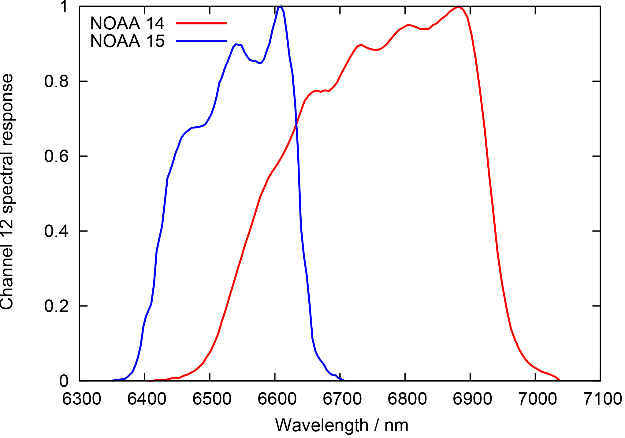
Figure 1Channel 12 spectral response functions of the HIRS 2 instrument on NOAA 14 and the HIRS 3 instrument on NOAA 15.
LibRadtran is used with the following set-up: we use the DISORT radiative transfer solver (Stamnes et al., 1988) with 16 discrete angles and the representative wavelengths band parameterisation (reptran, Gasteiger et al., 2014) with fine resolution (1 cm−1). We assume a ground albedo of zero and cloud-free scenes (as brightness temperatures from the Shi and Bates data set are cloud cleared, see Shi and Bates, 2011). The background profiles of the absorbing gases are taken from implemented standard atmosphere profiles (Anderson et al., 1986), whereby the appropriate profile is automatically selected from the geographical position and the time to which the radiosonde profile refers. We calculate the channel-integrated brightness temperatures at the top of the atmosphere for nadir and 30∘ off-nadir directions for these profiles.
The atmospheric profiles of temperature and relative humidity (with respect to liquid water) are taken from large sets of radiosonde data with high vertical resolution. (1) We use the set of profiles from the German weather observatory Lindenberg (52.21∘ N, 14.12∘ E, Spichtinger et al., 2003), similarly to earlier satellite studies (Gierens et al., 2004; Gierens and Eleftheratos, 2016). We use this set of more than 1500 profiles to derive a regression-based solution (our training data set). (2) To see whether there are also systematic differences between latitude zones radiosonde profiles from Sodankylä, Finland (67.37∘ N, 26.60∘ E) and Manus, Papua New Guinea (2.06∘ S, 146.93∘ E) are used. These weather observatories belong to the Global Climate Observing System (GCOS) Reference Upper-Air Network (GRUAN). The data and products of the GRUAN network are quality-controlled as described by Immler et al. (2010); Dirksen et al. (2014). We use 1 year of profiles from both stations: 2013 for Manus and 2014 for Sodankylä. These profiles were used for testing the regression that we derived from the Lindenberg profiles. The GRUAN profiles have a very high vertical resolution – too high for the radiative transfer calculation. Thus, only every 10th record has been used from the surface to 90 hPa. At higher altitudes (mainly in the dry stratosphere) we have replaced the radiosonde data by data from the standard atmospheres implemented in libRadtran.
Figure 2 displays the pseudo-channel 12 brightness temperatures for T12∕15 against the corresponding brightness temperature differences (NOAA 15 minus NOAA 14), ΔT12, computed with libRadtran for the Sodankylä and the Manus profiles. T12∕15 and ΔT12 are presented for nadir and 30∘ off-nadir directions. As expected, the brightness temperatures for the two considered viewing directions differ, and their difference is rather constantly about 1 to 2 K. More precisely, the summary statistics for the two locations are as follows. At Sodankylä the mean difference at nadir is −6.7 ± 1.2 K, and the mean difference at 30∘ is −6.7 ± 1.3 K. At Manus the mean difference at both nadir and at 30∘ are −7.1 ± 0.9 K. It is thus sufficient to only use the nadir radiances for further analyses. It can be noted that T12∕15 varies between 225 and 242 K for the Sodankylä profiles, while the corresponding ΔT12 ranges between −12 and −3 K. There is no obvious correlation between ΔT12 and T12∕15. For Manus, the data pairs show values of T12∕15 from roughly 229 to 241 K and brightness temperature differences ranging from −10 to −5 K. Again there is no obvious correlation between the brightness temperatures themselves and the corresponding differences.

Figure 2Scatter plot of brightness temperatures calculated with a radiative transfer model using radiosonde profiles from Sodankylä, Finland (a) and Manus, Papua New Guinea (b). The abscissa represents the brightness temperature obtained with a channel 12 spectral response function for HIRS/3 on NOAA 15. The ordinate represents the difference between this brightness temperature and a corresponding one computed using the channel 12 spectral response function for HIRS/2 on NOAA 14. The calculations have been performed for both nadir and 30∘ off-nadir viewing directions.
Figure 3a displays the corresponding results for the radiosonde profiles from Lindenberg. The data pairs form two groups: a large patch at low T12∕15 and a “tail” at small ΔT12 but higher T12∕15. This tail has been discarded from further analysis since inspection of the corresponding profiles showed that the relative humidity sensor was obviously malfunctioning in the middle and upper troposphere (and in the stratosphere), indicating zero relative humidity. 1558 profiles out of the total 1660 profiles remain for the analysis. Figure 3b shows the same data without the mentioned tail represented as a 2-D histogram. The data at the maximum frequency (dark blue) have a brightness temperature difference of about −7 K. Only a small set of the data pairs has K and an even smaller set has K.
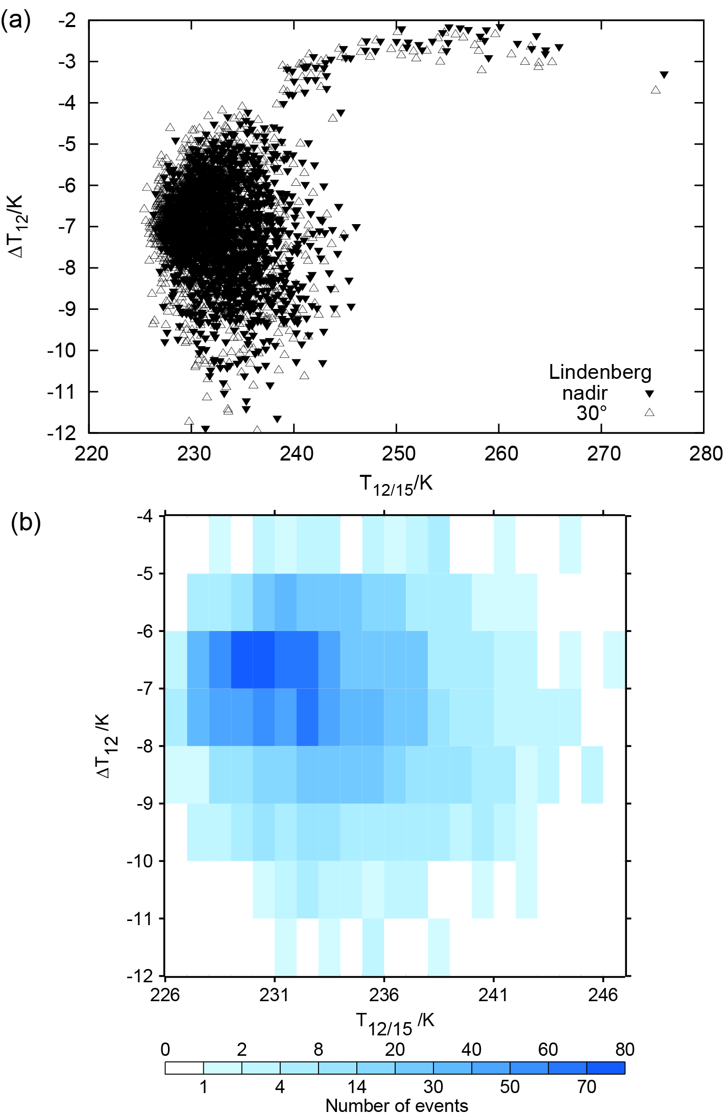
Figure 3(a) Scatter plot as in Fig. 2 and (b) corresponding 2-D histogram for channel 12 brightness temperatures computed using radiosonde profiles from Lindenberg, Germany. Note the tail of high values in the scatter plot results from profiles with a malfunctioning RH instrument. These 102 profiles have been discarded from further analysis. The 2-D frequency histogram does not contain them anymore. Calculations have been performed for nadir and 30∘ off-nadir directions, but the off-nadir results are only shown in the scatter plot.
At this point it is useful to recall that the weighting functions of the two considered channels peak at altitudes about 1 km apart because the water vapour optical thickness is larger at the central frequency of channel 12 on HIRS/3 than that on HIRS/2. The vertical distance of 1 km implies an air temperature difference of about 6.5 K on average in the upper troposphere, and this explains that an average ΔT12 of about the same value is found in the radiative transfer calculations. A similar (average) correction of 8 K has been derived by Shi and Bates (2011) and used by Chung et al. (2016).
Now the question arises of how characteristics of humidity profiles are reflected in the brightness temperature differences. Figure 4 shows three sets of relative humidity profiles: 5 profiles with K (panel a), 6 profiles with −7.21 K < K (panel b) and 20 profiles with a small difference, K (panel c). Note that relative humidity values are reported as integers in our data set, which explains the somewhat angular structure of some of the profiles.
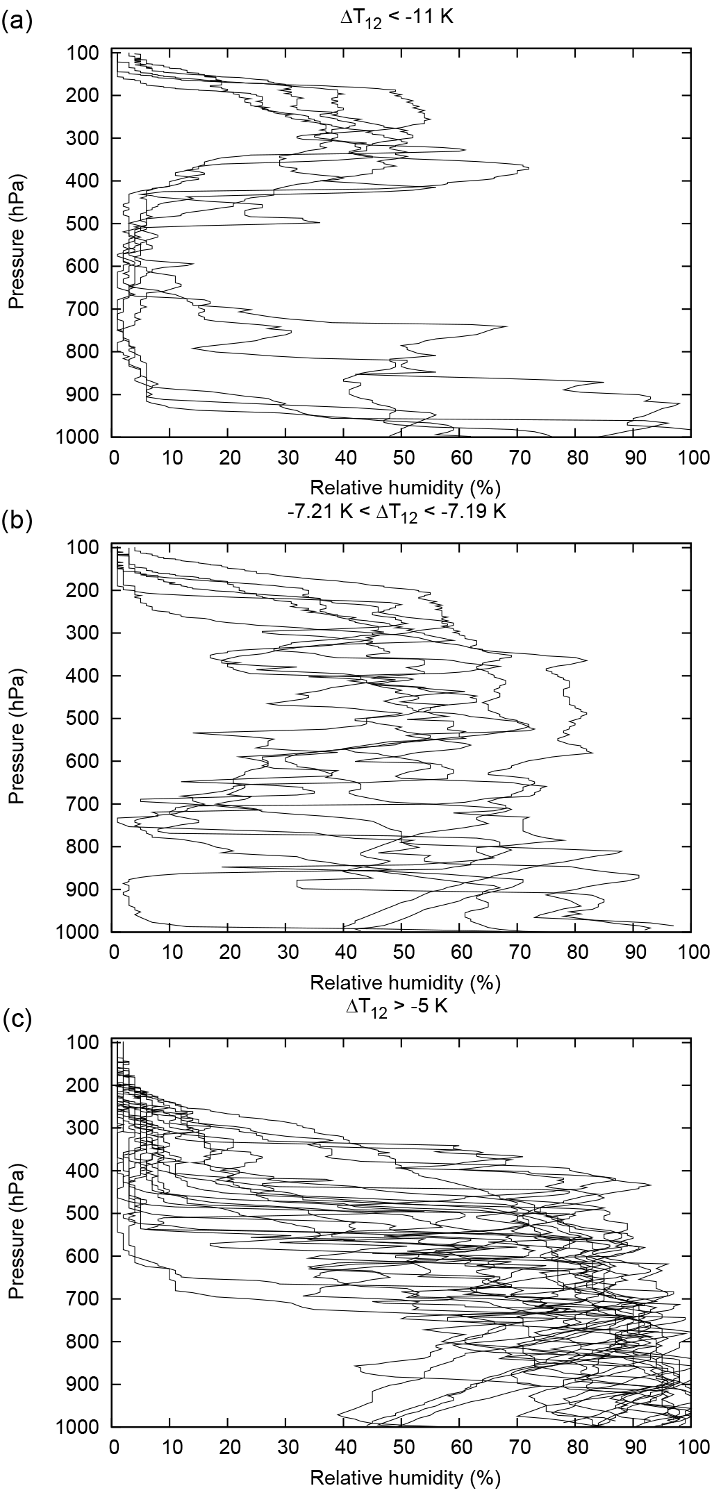
Figure 4Lindenberg radiosonde profiles of relative humidity vs. pressure altitude that lead to brightness temperature differences in extreme ranges (a, c, values indicated in the figures) and to values near to the mean (b). The profiles are obtained from the following launches (format yymmddhh): 00042806, 00122312, 01011506, 01021717, 01030712 (a); 00070112, 00111618, 00112318, 00123012, 01021612, 01040218 (b); 00021306, 00021312, 00021406, 00022100, 00022106, 00052912, 00053018, 00060706, 00071506, 00080112, 00080200, 00111606, 00121606, 01020118, 01020218, 01022206, 01022218, 01022306, 01022312, 01022400 (c).
The first set of profiles with K is characterised by high values of RH in the upper troposphere (200 to 400 hPa) and a very dry mid-troposphere (450 to 650 hPa). Accordingly, channel 12 on NOAA 15 (ch. 12/15) gets more radiance from the upper levels than channel 12 on NOAA 14 (ch. 12/14) because it is more sensitive there. In turn, ch. 12/14 cannot balance this deficit in the mid-tropospheric levels since it is too dry at this altitude. The result is a large negative difference in brightness temperatures. The profiles with K are in turn characterised by a mid-troposphere that has much higher relative humidity than the upper troposphere. Under this circumstance the peak of the ch. 12/15 weighting function approaches the peak of the ch. 12/14 weighting function; that is, the brightness temperatures become more similar. Finally, an average brightness temperature difference is found for profiles without a strong humidity contrast between the upper and the mid-tropospheric levels, as shown in Fig. 4b.
This analysis shows that one can understand from consideration of the underlying radiation physics why the brightness temperature differences sometimes obtain large or relatively small values and why the average difference is of the order of −7 K. It is, however, clear that this additional knowledge is not available when satellite data analysis is confined to channel 12 only. To exploit this knowledge one needs further pieces of information, in particular on the humidity in the mid-tropospheric levels. Fortunately, this knowledge is available from the same HIRS instruments, from channel 11 (see, e.g. Soden and Bretherton, 1996).
4.1 Regression using HIRS/3 channels 11 and 12
HIRS/3 channel 11 is centred at a wavelength of 7.3 µm. While the strong water vapour ν2 vibration–rotation band has its peak line strengths at about the channel 12 wavelength (≈6.5 µm), channel 11 is centred on the long-wave side of this band, off the peak with lower line strengths, and thus channel 11 is characteristic of the water vapour in lower levels than channel 12. In a standard midlatitude summer atmosphere channel 11 peaks at about 5 km altitude (see Fig. 2 of Gierens and Eleftheratos, 2016).
Using the channel spectral response function for channel 11 on NOAA 15, radiative transfer calculations have been performed for the radiosonde profiles used above. Figure 5 shows the resulting brightness temperatures, T11∕15, plotted against the previously computed ΔT12 for the set of Lindenberg profiles. As expected, T11∕15 is generally higher than the channel 12 brightness temperatures because it characterises the temperature in the mid-troposphere where the channel 11 weighting function peaks. T11∕15 ranges from 248 to 268 K for the Lindenberg profiles. Figure 5 also shows a linear correlation between ΔT12 and T11∕15, although with a large scatter. The linear Pearson correlation coefficient is −0.68. Its square is 0.46, that is, variations of T11∕15 represent almost half of the variations in ΔT12. The remaining scatter is not surprising given the tremendous variability of relative humidity profiles. One additional piece of information is clearly insufficient to capture all this variability. Nevertheless, the correlation is clearly visible. We have made use of it to construct a correction to the HIRS/3 measured channel 12 brightness temperatures, a correction that leads to a pseudo-channel 12 brightness temperature as if a HIRS/2 instrument had measured it.
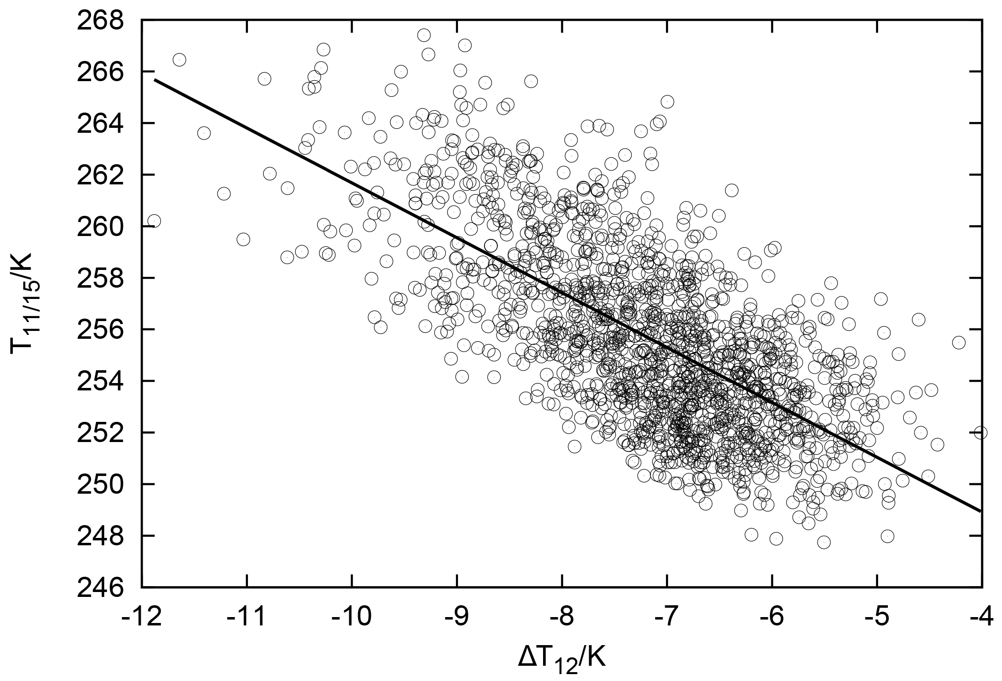
Figure 5Scatter plot showing a linear correlation for the difference between channel 12 brightness temperatures (NOAA 15 minus NOAA 14) and the NOAA 15 channel 11 brightness temperature computed using the Lindenberg profiles. The linear Pearson correlation coefficient is −0.68.
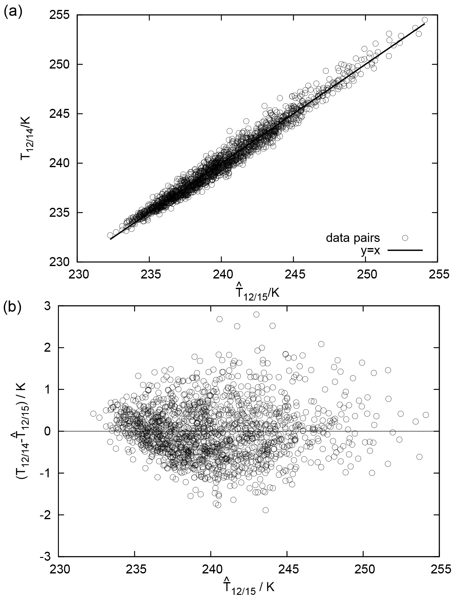
Figure 6(a) Scatter plot showing a linear correlation between a linear superposition of channel 11 and 12 brightness temperatures from NOAA 15 (abscissa, ) with the corresponding channel 12 brightness temperature for the same profile but computed with the NOAA 14 channel response function. Note that the fit line has slope 1.000 and the intercept is close to zero (). The linear correlation is R=0.986. All data are computed using the Lindenberg profiles. (b) The same data, plotted with the difference in on the y axis.
For this purpose we try a bilinear regression 2 of the following kind:
Here, is the desired pseudo-channel 12 brightness temperature that is equivalent to a HIRS/2 measurement. In other words it is the T12∕15 that would have been measured by a HIRS/2 instrument. For the calculation of only the nadir brightness temperatures have been retained as it seems that the off-nadir directions do not yield differing information. The two data vectors containing the brightness temperatures of channels 11 and 12 are linearly correlated with R=0.71, but they point in different directions; that is, they are not co-linear. Regression thus yields a unique result, namely
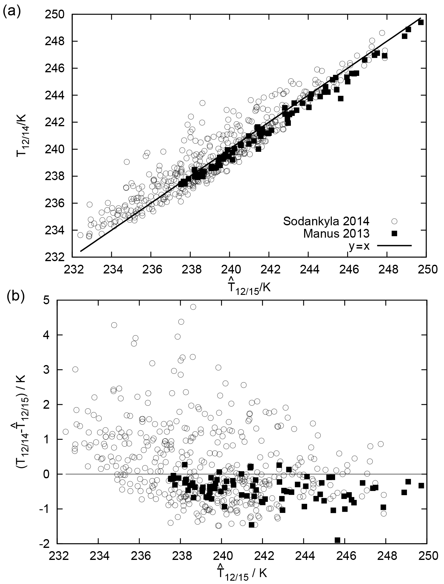
Figure 7(a) Test of the superposition method using radiosonde profiles from the two GRUAN stations Sodankylä, Finland, and Manus, Papua New Guinea. The diagonal line (y=x) is included to check the result: it is not a fit. (b) The same data, plotted with the difference in on the y axis.
The 1 σ uncertainty estimates of the parameters b,c are both ±0.01. The corresponding data pairs are shown in Fig. 6. The slope and intercept of the regression (black line in panel a) are 1.000 and , respectively, and the linear correlation between the linear superposition of channel 11 and 12 brightness temperatures and that of the pseudo-channel 12 brightness temperature is 0.986. Panel (b) shows the same data but with the difference between regressand and regressor on the y axis. Maximum deviations from the zero line are about +3 and −2 K. Mean and standard deviation of the residuals are 0.0±0.6 K.
4.2 Test with independent radiosonde profiles
Using the linear superposition of channel 11 and 12 brightness temperatures for the considered atmospheric profiles from the two GRUAN stations, Sodankylä and Manus, leads to the data pairs shown in Fig. 7. The black diagonal line in this figure is not the result of a best fit or a regression, but is y=x, plotted to guide the eye in checking the result. The residual means () and their standard deviations are 0.3±1.3 K for Sodankylä and K for Manus. Again, we see that the regression using just one additional piece of information is not able to provide a complete correction with an average residual of zero. At least these residuals are much smaller than the original differences between T12∕14 and T12∕15 shown in Fig. 2. Obviously, the superposition methods works well for these data, representing a polar and an equatorial atmosphere.
5.1 Superposition of weighting functions
The superposition of channels 11 and 12 is equivalent to a superposition of their weighting functions. Fig. 8 gives an example. The weighting functions are generic functions, as in Gierens and Eleftheratos (2016), assuming a water vapour scale height of 2 km and peak altitudes of 8.5 km for ch. 12/15 (red curve), 7.5 km for ch. 12/14 (black) and 5 km for ch. 11/15 (blue). The black curve with circles represents the superposition of channels 11 and 12 on NOAA 15 with the weights b and c derived above. The superposition curve (its upper tail, its peak and about half of its lower tail) is between the corresponding channel 12 weighting functions. We note here that the superposition weighting function has some weight at lower altitudes where both channel 12 weighting functions are already very low. Overall, we see that the superposition method eventually brings the pseudo-channel 12 brightness temperature of NOAA 15 closer to the level of the corresponding channel 12 brightness temperature of NOAA 14.
Figure 8 (and actual weighting functions shown in the Supplement, Fig. S1) shows that there is some possibility that channel 11 sees the ground when the atmosphere is quite dry. In such cases, which might occur at high latitudes, the superposition will not work. High brightness temperatures in both channels 10 and 11 could indicate such an event. Indeed, the (high-latitude) Sodankylä data show larger scatter in Fig. 7 than the (equatorial) data from Manus, which might result from unwanted ground influence at the high-latitude station.
An interesting alternative interpretation of the coefficients resulting from the bilinear regression may derive from the following consideration: it is possible to rewrite Eq. (1) as a weighted mean of three temperatures:
From this interpretation and Eq. (2) follows and it turns out that T0=241.6 K, which is remarkably close to 240 K, the T0 used as a reference in the retrieval schemes developed by Soden and Bretherton (1993), Stephens et al. (1996) and Jackson and Bates (2001). At the altitude where the channel 12 weighting function peaks the temperature is, on average, close to T0. The remarkable fact is that the regression results just in this T0 for the constant part and not anything else – a finding that could not be expected a priori.
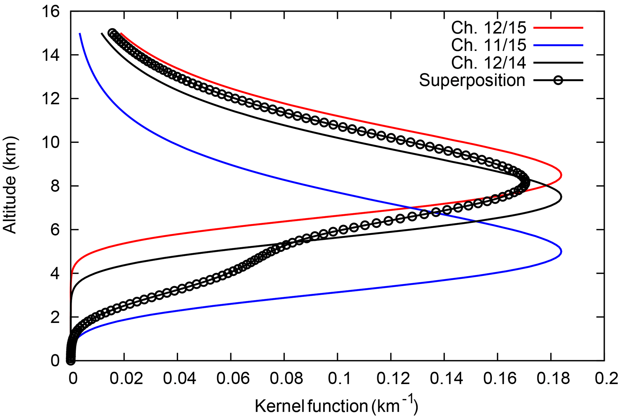
Figure 8Examples of weighting functions for channels 11 and 12 on NOAA 15 (blue and red), their superposition (black with circles) and channel 12 on NOAA 14 (black).
5.2 Application to real data
For the same set of 1004 days of common operation of NOAA 14 and NOAA 15 as used in GE17, we have compared the channel 12 brightness temperatures and daily averages on a 2.5∘ × 2.5∘ grid in the northern midlatitudes, 30 to 70∘ N. Differing from the previous paper, we use the original non-intercalibrated brightness temperatures. For NOAA 15 we compute the linear superposition derived above, that is, , while for NOAA 14 we use T12,14. The 2-D histogram of these data pairs is shown in Fig. 9. It is remarkable how similar this histogram is to a corresponding one shown as Fig. 2 in GE17, which displays the intercalibrated data. The ordinary least squares linear fit through the new data pairs (solid line) has the equation:
with a slightly smaller slope and a slightly larger intercept than in GE17 using the intercalibrated data pairs (0.8290 and 41.63, respectively). These coefficients have been determined using a non-linear least-squares Marquardt–Levenberg algorithm (Press et al., 1989, chap. 14.4). The slope has a 1σ uncertainty of 0.001. Because the linear least squares fit suffers from regression dilution when errors of the regressor () are not taken into account, we also compute the bivariate regression (dash-dotted), which has the equation:
and this has a slightly smaller slope and larger intercept than the corresponding fit through the intercalibrated data (which has 0.994 and 2.007, respectively). As such the quoted uncertainty of the slope coefficient (0.001) refers only to the ordinary least squares fit. The difference between the slope coefficients of the ordinary and bivariate regression is considerably larger than the error estimate given above (i.e. 0.8025 vs. 0.9256). If we take this difference as a measure of uncertainty of the slope parameter, then the differences between the present parameters and those in GE17 (i.e. 0.8025 vs. 0.8290 for the ordinary least squares and 0.9256 vs. 0.994 for the bivariate regression) are relatively small. In this sense we may state that this comparison remarkably shows that two essentially different methods used to treat the HIRS 2 to HIRS 3 transition lead to very similar results.
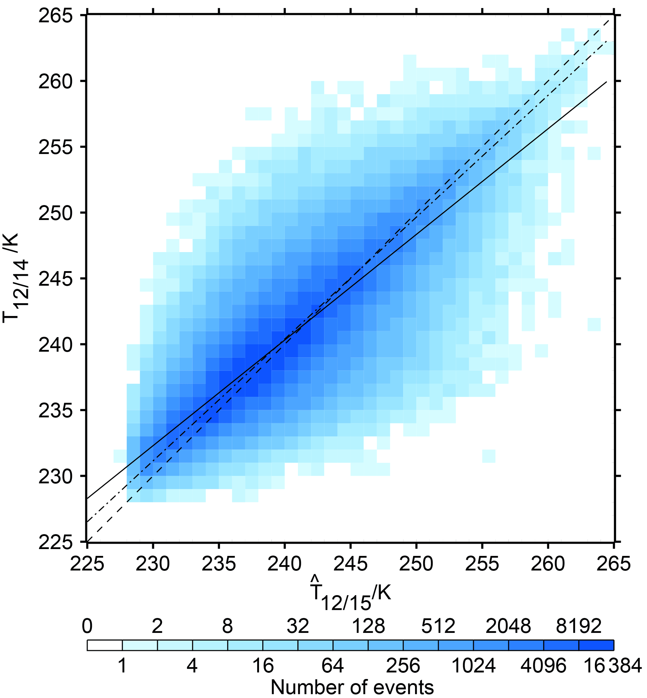
Figure 92-D histogram of brightness temperatures, displaying on the abscissa and T12∕14 on the ordinate axes. The data are from 1004 common days of operation of NOAA 14 and NOAA 15. The dashed diagonal line represents x=y, the solid line is the best fit according to an ordinary least squares regression and the dashed–dotted line is the bivariate regression line.
In pursuit of the goal to study changes in upper-tropospheric humidity with respect to ice (UTHi) we applied the retrieval formula of Jackson and Bates (2001) to and to T12,14 of the common 1004 days. A density plot of the corresponding data pairs of UTHi is displayed in Fig. 10. Obviously the result is not satisfying; the plot closely resembles the corresponding scatter of data pairs produced from the intercalibrated data (Shi and Bates, 2011) that are shown in Fig. 1 of GE17. Unfortunately the superposition method does not solve the problem of a considerable overestimation of the number of supersaturation events recorded with HIRS 3 and 4 instruments and it seems that the pseudo-channel 12 data have to be treated with the cdf-matching technique developed by GE17 in the same way as the intercalibrated data. This is beyond the scope of the present paper.
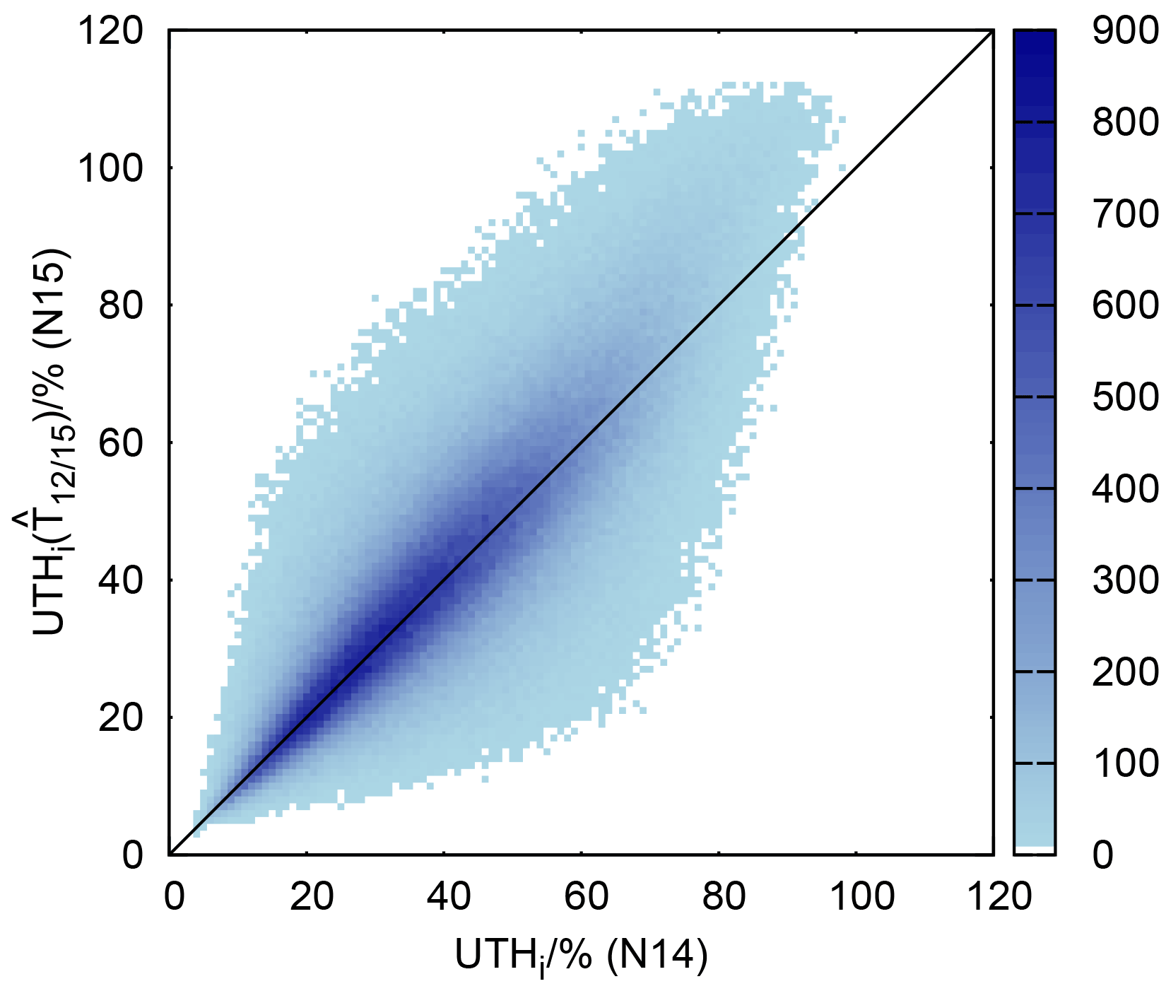
Figure 10Heat map displaying UTHi computed using on the ordinate against values computed from the original T12∕14 on the abscissa. Obviously the problem concerning the excess of supersaturation cases in the NOAA 15 data remains even with this new kind of data treatment. The colour scale shows the number of events in each 1 % × 1 % pixel.
The new method is an independent approach for an intercalibrated HIRS channel 12 data set, based on results of radiative transfer calculations, classification of profile characteristics and a superposition with information delivered by channel 11. The intercalibration of Shi and Bates (2011) is instead based on pixelwise direct corrections, where the brightness temperature-dependent corrections are determined from regressions of the first kind between subsequent satellite pairs. As Figs. 9 and 10 show, both methods seem to produce very similar results. The statistically based method of Shi and Bates (2011) is thus supported by an independent method, and results obtained from data intercalibrated with either method should be more trustworthy. We thus consider our question from the beginning to be answered positively: whether combining HIRS 2 and HIRS 3 data into a single time series is justified. Although both methods produce similar results, as we see in Fig. 10, neither method of intercalibration solves the problems with the discrepancy in the range of high UTHi values which results from a corresponding discrepancy at the low tail of channel 12 brightness temperatures (see GE17). It is probable that this problem does not originate from the intercalibration procedure, since for the radiative transfer calculation it makes no difference whether the humidity profile contains a very humid upper troposphere with supersaturated layers or not. In each case it provides the corresponding brightness temperature. It is more probable that the problem with the lower tail of the T12 distribution comes from the retrieval method, which is based on linearisations around certain “tangential points”, thermodynamic properties typical of the upper troposphere (e.g. the T0=240 K mentioned above) and that this linear approach is not completely sufficient in cases in which actual properties are too far away from the tangential points.
The procedure we have developed in the present paper follows these steps:
-
The difference, , calculated with libRadtran for a set of radiosonde profiles, ranges from −12 to −4 K, with most cases around −7 K, which fits to the approximately 1 km altitude difference between the peaks of the channel 12 weighting functions of HIRS/2 and HIRS/3.
-
It turns out that the shape of the RH profile determines whether ΔT12 is close to one of the extremes or close to the average. It is particularly the shape of the humidity profile in the lower to mid-troposphere that plays a role here.
-
Take channel 11 brightness temperatures as a proxy of that part of the profile, as that channel measures the humidity in the lower to mid-troposphere.
-
Indeed, and fortunately, T11∕15 is correlated to ΔT12; thus it can be used to identify in which cases ΔT12 is large, average or small.
-
Thus it is possible to find a correction to T12∕15 such that the result is close to (with a mean residual difference of about 1 K) the brightness temperature that N14 would have measured if it had seen the same scene. This correction is a linear superposition of T12∕15 and T11∕15, measured by the same HIRS instrument.
Application of this superposition method to real data of 1004 common days of operation of NOAA 14 and NOAA 15, comparing T12∕14 with the pseudo-channel 12 brightness temperature of NOAA 15, , yields a 2-D distribution that is very similar to the corresponding distribution obtained with the intercalibrated brightness temperatures from Shi and Bates (2011). Comparing the corresponding values of UTHi again yields a 2-D distribution very similar to that obtained from the intercalibrated data. From these findings we conclude that our method, which is based on radiative transfer calculations, i.e. physics, produces very similar results with the Shi and Bates statistical intercalibration method. The justification to use the intercalibrated channel 12 time series including its early HIRS 2 and later HIRS 3 and 4 phases is thus corroborated.
Note that this paper only shows the principle of method, how a pseudo HIRS/2 channel 12 brightness temperature can be computed from later HIRS versions, involving channels 11 and 12. As all HIRS instruments have slightly different channel spectral response functions, the regression parameters (a, b, c) will differ from one instrument pair to the other. They will also depend on which HIRS/2 instrument serves as reference. In this paper we used HIRS/2 on NOAA 14, but it certainly makes sense to additionally use HIRS/2 on NOAA 12 as Shi and Bates (2011) based their intercalibration on that satellite. This work is beyond the scope of the current paper and left for future exercise. We also note that this analysis represents a relatively short period in the lifetime of two HIRS instruments and that their spectral and radiometric calibration was assumed to be constant over this period.
The libRadtran radiative transfer software package is freely available under the GNU General Public License from http://www.libradtran.org/doku.php.
The GRUAN radiosonde data are available from the GRUAN websites. The special Lindenberg radiosonde data set is available from the first author on request. The NOAA satellite data are available from NOAA public websites.
The supplement related to this article is available online at: https://doi.org/10.5194/amt-11-939-2018-supplement.
KG made the radiative transfer calculations and the analyses. KG and RS discussed the procedures and the statistical methods. KE prepared the satellite data in a useful form. All authors contributed to the text.
The authors declare no competing interests.
The authors thank the LibRadtran developer team for providing the
radiative transfer code and Luca Bugliaro for checking the first
author's set-up of the radiative transfer job. We are grateful to all
the people who provided the data used in this paper, who are
colleagues from NOAA, the GRUAN network and DWD. Christoph Kiemle
read the pre-final version of the manuscript and made good
suggestions for improvement and further discussion. Thanks for this!
The article processing charges for this open-access
publication were covered by a Research
Centre of the Helmholtz Association.
Edited by: Isaac Moradi
Reviewed by: two
anonymous referees
Anderson, G., Clough, Kneizys, F., Chetwynd, J., and Shettle, E.: AFGL atmospheric constituent profiles (0–120 km), Tech. Rep. Tech. Rep. AFGL-TR-86-0110, Air Force Geophys. Lab., Hanscom Air Force Base, Bedford, Mass., 1986. a
Chung, E.-S., Soden, B., Huang, X., Shi, L., and John, V.: An assessment of the consistency between satellite measurements of upper tropospheric water vapor, J. Geophys. Res., 121, 2874–2887, https://doi.org/10.1002/2015JD024496, 2016. a, b
Dirksen, R. J., Sommer, M., Immler, F. J., Hurst, D. F., Kivi, R., and Vömel, H.: Reference quality upper-air measurements: GRUAN data processing for the Vaisala RS92 radiosonde, Atmos. Meas. Tech., 7, 4463–4490, https://doi.org/10.5194/amt-7-4463-2014, 2014. a
Emde, C., Buras-Schnell, R., Kylling, A., Mayer, B., Gasteiger, J., Hamann, U., Kylling, J., Richter, B., Pause, C., Dowling, T., and Bugliaro, L.: The libRadtran software package for radiative transfer calculations (version 2.0.1), Geosci. Model Dev., 9, 1647–1672, https://doi.org/10.5194/gmd-9-1647-2016, 2016. a
Gasteiger, J., Emde, C., Mayer, B., Buehler, S., and Lemke, O.: Representative wavelengths absorption parameterization applied to satellite channels and spectral bands, J. Quant. Spectrosc. Ra., 148, 99–115, 2014. a
Gierens, K. and Eleftheratos, K.: Upper tropospheric humidity changes under constant relative humidity, Atmos. Chem. Phys., 16, 4159–4169, https://doi.org/10.5194/acp-16-4159-2016, 2016. a, b, c
Gierens, K. and Eleftheratos, K.: Technical note: On the intercalibration of HIRS channel 12 brightness temperatures following the transition from HIRS 2 to HIRS 3/4 for ice saturation studies, Atmos. Meas. Tech., 10, 681–693, https://doi.org/10.5194/amt-10-681-2017, 2017. a
Gierens, K., Kohlhepp, R., Spichtinger, P., and Schroedter-Homscheidt, M.: Ice supersaturation as seen from TOVS, Atmos. Chem. Phys., 4, 539–547, https://doi.org/10.5194/acp-4-539-2004, 2004. a
Gierens, K., Eleftheratos, K., and Shi, L.: Technical Note: 30 years of HIRS data of upper tropospheric humidity, Atmos. Chem. Phys., 14, 7533–7541, https://doi.org/10.5194/acp-14-7533-2014, 2014. a
Immler, F. J., Dykema, J., Gardiner, T., Whiteman, D. N., Thorne, P. W., and Vömel, H.: Reference Quality Upper-Air Measurements: guidance for developing GRUAN data products, Atmos. Meas. Tech., 3, 1217–1231, https://doi.org/10.5194/amt-3-1217-2010, 2010. a
Jackson, D. and Bates, J.: Upper tropospheric humidity algorithm assessment, J. Geophys. Res., 106, 32259–32270, 2001. a, b
Press, W., Flannery, B., Teukolsky, S., and Vetterling, W.: Numerical recipes, Cambridge University Press, Cambridge, UK, 1989. a
Shi, L. and Bates, J.: Three decades of intersatellite–calibrated High–Resolution Infrared Radiation Sounder upper tropospheric water vapor, J. Geophys. Res., 116, D04108, https://doi.org/10.1029/2010JD014847, 2011. a, b, c, d, e, f, g, h, i, j, k
Soden, B. and Bretherton, F.: Upper tropospheric relative humidity from the GOES 6.7 µm channel: Method and climatology for July 1987, J. Geophys. Res., 98, 16669–16688, 1993. a
Soden, B. and Bretherton, F.: Interpretation of TOVS water vapor radiances in terms of layer–averaged relative humidities: Method and climatology for the upper, middle, and lower troposphere, J. Geophys. Res., 101, 9333–9343, 1996. a, b
Spichtinger, P., Gierens, K., Leiterer, U., and Dier, H.: Ice supersaturation in the tropopause region over Lindenberg, Germany, Meteorol. Z., 12, 143–156, 2003. a
Stamnes, K., Tsay, S.-C., Wiscombe, W., and Jayaweera, K.: Numerically stable algorithm for discrete ordinate method radiative transfer in multiple scattering and emitting layered media, Appl. Optics, 27, 2502–2509, 1988. a
Stephens, G., Jackson, D., and Wittmeyer, I.: Global observations of upper–tropospheric water vapor derived from TOVS radiance data, J. Climate, 9, 305–326, 1996. a
Satellite Application Facility (SAF) for numerical weather prediction (NWP) https://nwpsaf.eu/site/software/rttov/download/coefficients/spectral-response-functions, last access in March 2017
The regression
has been performed using IDL (Interactive Data Language) routine
REGRESS.
- Abstract
- Introduction
- Radiative transfer simulations of channel 12 radiation for HIRS/2 and HIRS/3
- Discussion of radiative transfer results
- Construction of a pseudo HIRS/2 channel 12
- Discussion
- Conclusions
- Code availability
- Data availability
- Author contributions
- Competing interests
- Acknowledgements
- References
- Supplement