the Creative Commons Attribution 4.0 License.
the Creative Commons Attribution 4.0 License.
 | 02 Jan 2019
Improved aerosol correction for OMI tropospheric NO2 retrieval over East Asia: constraint from CALIOP aerosol vertical profile
Mengyao Liu
K. Folkert Boersma
Gaia Pinardi
Yang Wang
Julien Chimot
Thomas Wagner
Pinhua Xie
Henk Eskes
Michel Van Roozendael
François Hendrick
Pucai Wang
Ting Wang
Yingying Yan
Lulu Chen
Ruijing Ni
Satellite retrieval of vertical column densities (VCDs) of tropospheric nitrogen dioxide (NO2) is critical for NOx pollution and impact evaluation. For regions with high aerosol loadings, the retrieval accuracy is greatly affected by whether aerosol optical effects are treated implicitly (as additional “effective” clouds) or explicitly, among other factors. Our previous POMINO algorithm explicitly accounts for aerosol effects to improve the retrieval, especially in polluted situations over China, by using aerosol information from GEOS-Chem simulations with further monthly constraints by MODIS/Aqua aerosol optical depth (AOD) data. Here we present a major algorithm update, POMINO v1.1, by constructing a monthly climatological dataset of aerosol extinction profiles, based on level 2 CALIOP/CALIPSO data over 2007–2015, to better constrain the modeled aerosol vertical profiles.
We find that GEOS-Chem captures the month-to-month variation in CALIOP aerosol layer height (ALH) but with a systematic underestimate by about 300–600 m (season and location dependent), due to a too strong negative vertical gradient of extinction above 1 km. Correcting the model aerosol extinction profiles results in small changes in retrieved cloud fraction, increases in cloud-top pressure (within 2 %–6 % in most cases), and increases in tropospheric NO2 VCD by 4 %–16 % over China on a monthly basis in 2012. The improved NO2 VCDs (in POMINO v1.1) are more consistent with independent ground-based MAX-DOAS observations (R2=0.80, NMB = −3.4 %, for 162 pixels in 49 days) than POMINO (R2=0.80, NMB = −9.6 %), DOMINO v2 (R2=0.68, NMB = −2.1 %), and QA4ECV (R2=0.75, NMB = −22.0 %) are. Especially on haze days, R2 reaches 0.76 for POMINO v1.1, much higher than that for POMINO (0.68), DOMINO v2 (0.38), and QA4ECV (0.34). Furthermore, the increase in cloud pressure likely reveals a more realistic vertical relationship between cloud and aerosol layers, with aerosols situated above the clouds in certain months instead of always below the clouds. The POMINO v1.1 algorithm is a core step towards our next public release of the data product (POMINO v2), and it will also be applied to the recently launched S5P-TROPOMI sensor.


Air pollution is a major environmental problem in China. In particular, China has become the world's largest emitter of nitrogen oxides (NOx = NO+NO2) due to its rapid economic growth, heavy industries, coal-dominated energy sources, and relatively weak emission control (Zhang et al., 2009; Lin et al., 2014a; Cui et al., 2016; Stavrakou et al., 2016). Tropospheric vertical column densities (VCDs) of nitrogen dioxide (NO2) retrieved from the Ozone Monitoring Instrument (OMI) on board the Earth Observing System (EOS) Aura satellite have been widely used to monitor and analyze NOX pollution over China because of their high spatiotemporal coverage (e.g., Zhao and Wang, 2009; Lin et al., 2010; Miyazaki and Eskes, 2013; Verstraeten et al., 2015). However, NO2 retrieved from OMI and other spaceborne instruments is subject to errors in the conversion process from radiance to VCD, particularly with respect to the calculation of tropospheric air mass factor (AMF) that is used to convert tropospheric slant column density (SCD) to VCD (e.g., Boersma et al., 2011; Bucsela et al., 2013; Lin et al., 2015; Lorente et al., 2017).
Most current-generation NO2 algorithms do not explicitly account for the effects of aerosols on NO2 AMFs and on prerequisite cloud parameter retrievals. These retrievals often adopt an implicit approach wherein cloud algorithms retrieve “effective cloud” parameters that include the optical effects of aerosols. This implicit method is based on aerosols exerting an effect on the top-of-atmosphere radiance level, whereas the assumed cloud model does not account for the presence of aerosols in the atmosphere (Stammes et al., 2008; P. Wang et al., 2008; Wang and Stammes, 2014; Veefkind et al., 2016). In the absence of clouds, an aerosol optical thickness of 1 is then interpreted as an effective cloud fraction of ±0.10, and the value also depends on the aerosol properties (scattering or absorbing), true surface albedo, and geometry angles (Chimot et al., 2016) with an effective cloud pressure closely related to the aerosol layer, at least for aerosols of predominantly scattering nature (e.g., Boersma et al., 2004, 2011; Castellanos et al., 2014, 2015). However, in polluted situations with high aerosol loadings and more absorbing aerosol types, which often occur over China and many other developing regions, the implicit method can result in considerable biases (Castellanos et al., 2014, 2015; Kanaya et al., 2014; Lin et al., 2014b; Chimot et al., 2016).
Lin et al. (2014b, 2015) established the POMINO NO2 algorithm, which builds on the DOMINO v2 algorithm (for OMI NO2 slant columns and stratospheric correction), but improves upon it through a more sophisticated AMF calculation over China. In POMINO, the effects of aerosols on cloud retrievals and NO2 AMFs are explicitly accounted for. In particular, daily information on aerosol optical properties such as aerosol optical depth (AOD), single scattering albedo (SSA), phase function, and vertical extinction profiles is taken from nested Asian GEOS-Chem v9-02 simulations. The modeled AOD at 550 nm is further constrained by MODIS/Aqua monthly AOD, with the correction applied to other wavelengths based on modeled aerosol refractive indices (Lin et al., 2014b). However, the POMINO algorithm does not include an observation-based constraint on the vertical profile of aerosols, whose altitude relative to NO2 has strong and complex influences on NO2 retrieval (Leitão et al., 2010; Lin et al., 2014b; Castellanos et al., 2015). This study improves upon the POMINO algorithm by incorporating CALIOP monthly climatology of aerosol vertical extinction profiles to correct for model biases.
The CALIOP lidar, carried on the sun synchronous CALIPSO satellite, has been acquiring global aerosol extinction profiles since June 2006 (Winker et al., 2010). CALIPSO and Aura are both parts of the National Aeronautics and Space Administration (NASA) A-Train constellation of satellites. The overpass time of CALIOP/CALIPSO is only 15 min later than OMI/Aura. In spite of issues with the detection limit, radar ratio selection, and cloud contamination that cause some biases in CALIOP aerosol extinction vertical profiles (Koffi et al., 2012; Winker et al., 2013; Amiridis et al., 2015), comparisons of aerosol extinction profiles between ground-based lidar and CALIOP show good agreements (Kim et al., 2009; Misra et al., 2012; Kacenelenbogen et al., 2014). However, CALIOP is a nadir-viewing instrument that measures the atmosphere along the satellite ground track with a narrow field of view. This means that the daily geographical coverage of CALIOP is much smaller than that of OMI. Thus previous studies often used monthly or seasonal regional mean CALIOP data to study aerosol vertical distributions or to evaluate model simulations (Chazette et al., 2010; Sareen et al., 2010; Johnson et al., 2012; Koffi et al., 2012; Ma and Yu, 2014).
There are a few CALIOP level 3 gridded datasets, such as LIVAS (Amiridis et al. 2015) and the NASA official level 3 monthly dataset (Winker et al., 2013, last access: March 2017). However, LIVAS is an annual average day–night combined product, not suitable to be applied to OMI NO2 retrievals (around early afternoon and in need of a higher temporal resolution than annual mean). The horizontal resolution (2∘ long × 5∘ lat) of the NASA official product is much coarser than OMI footprints and the GEOS-Chem model resolution.
Here we construct a custom monthly climatology of aerosol vertical extinction profiles based on 9 years (2007–2015) worth of CALIOP version 3 level 2 532 nm data. On a climatological basis, we use the CALIOP monthly data to adjust GEOS-Chem profiles in each grid cell for each day of the same month in any year. We then use the corrected GEOS-Chem vertical extinction profiles in the retrievals of cloud parameters and NO2. Finally, we evaluate our updated POMINO retrieval (hereafter referred to as POMINO v1.1), our previous POMINO product, DOMINO v2, and the newly released Quality Assurance for Essential Climate Variables product (QA4ECV; see Appendix A), using ground-based MAX-DOAS NO2 column measurements at three urban/suburban sites in East China for the year of 2012 and several months in 2008–2009.
Section 2 describes the construction of CALIOP aerosol extinction vertical profile monthly climatology, the POMINO v1.1 retrieval approach, and the MAX-DOAS data. It also presents the criteria for comparing different NO2 retrieval products and for selecting coincident OMI and MAX-DOAS data. Section 3 compares our CALIOP climatology with NASA's official level 3 CALIOP dataset and GEOS-Chem simulation results. Sections 4 and 5 compare POMINO v1.1 to POMINO to analyze the influence of improved aerosol vertical profiles on retrievals of cloud parameters and NO2 VCDs, respectively. Section 6 evaluates POMINO, POMINO v1.1, DOMINO v2, and QA4ECV NO2 VCD products using the MAX-DOAS data. Section 7 concludes our study.
2.1 CALIOP monthly mean extinction profile climatology
CALIOP is a dual-wavelength polarization lidar measuring attenuated backscatter radiation at 532 and 1064 nm since June 2006. The vertical resolution of aerosol extinction profiles is 30 m below 8.2 km and 60 m up to 20.2 km (Winker et al., 2013), with a total of 399 sampled altitudes. The horizontal resolution of CALIOP scenes is 335 m along the orbital track and is given over a 5 km horizontal resolution in level 2 data.
As detailed in Appendix B, we use the daily all-sky version 3 CALIOP level 2 aerosol profile product (https://search.earthdata.nasa.gov/search?q=CALIOP aerosol&ok=CALIOP, last access: April 2017) aerosol at 532 nm from 2007 to 2015 to construct a monthly level 3 climatological dataset of aerosol extinction profiles over China and nearby regions. This dataset is constructed on the GEOS-Chem model grid (0.667∘ long × 0.5∘ lat) and vertical resolution (47 layers, with 36 layers or so in the troposphere). The ratio of climatological monthly CALIOP to monthly GEOS-Chem profiles represents the scaling profile to adjust the daily GEOS-Chem profiles in the same month (see Sect. 2.2)
2.2 POMINO v1.1 retrieval approach
The NO2 retrieval consists of three steps. First, the total NO2 SCD is retrieved using the differential optical absorption spectroscopy (DOAS) technique (for the 405–465 nm spectral window in the case of OMI). The uncertainty of the SCD is determined by the appropriateness of the fitting technique, the instrument noise, the choice of fitting window, and the orthogonality of the absorbers' cross sections (Bucsela et al., 2006; Lerot et al., 2010; Richter et al., 2011; van Geffen et al., 2015; Zara et al., 2018). The NO2 SCD in DOMINO v2 has a bias at about 0.5–1.3 ×10¹⁵ molec. cm−2 (Dirksen et al., 2011; Belmonte Rivas et al., 2014; Marchenko et al., 2015; van Geffen et al., 2015; Zara et al., 2018), which can be reduced by improving wavelength calibration and including O2–O2 and liquid water absorption in the fitting model (van Geffen et al., 2015; Zara et al., 2018). The tropospheric SCD is then obtained by subtracting the stratospheric SCD from the total SCD. The bias in the total SCD is mostly absorbed by this stratospheric separation step, which may not propagate into the tropospheric SCD (van Geffen et al., 2015). The last step converts the tropospheric SCD to VCD by using the tropospheric AMF (VCD = SCD/AMF). The tropospheric AMF is calculated at 438 nm by using look-up tables (in most retrieval algorithms) or online radiative transfer modeling (in POMINO) driven by ancillary parameters, which act as the dominant source of errors in retrieved NO2 VCD data over polluted areas (Boersma et al., 2007; Lin et al., 2014b, 2015; Lorente et al., 2017).
Our POMINO algorithm focuses on the tropospheric AMF calculation over China and nearby regions, taking the tropospheric SCD (Dirksen et al., 2011) from DOMINO v2 (Boersma et al., 2011). POMINO improves upon the DOMINO v2 algorithm in the treatment of aerosols, surface reflectance, online radiative transfer calculations, spatial resolution of NO2, temperature and pressure vertical profiles, and consistency between cloud and NO2 retrievals (Lin et al., 2014b, 2015). In brief, we use the parallelized LIDORT-driven AMFv6 package to derive both cloud parameters and tropospheric NO2 AMFs for individual OMI pixels online (rather than using a look-up table). NO2 vertical profiles, aerosol optical properties, and aerosol vertical profiles are taken from the nested GEOS-Chem model over Asia (0.667∘ long × 0.5∘ lat before May 2013 and 0.3125∘ long × 0.25∘ lat afterwards), and pressure and temperature profiles are taken from the GEOS-5- and GEOS-FP-assimilated meteorological fields that drive GEOS-Chem simulations. Model aerosols are further adjusted by satellite data (see below). We adjust the pressure profiles based on the difference in elevation between the pixel center and the matching model grid cell (Zhou et al., 2010). We also account for the effects of surface bidirectional reflectance distribution function (BRDF) (Zhou et al., 2010; Lin et al., 2014b) by taking three kernel parameters (isotropic, volumetric, and geometric) from the MODIS MCD43C2 dataset (https://search.earthdata.nasa.gov/search?q=MODIS MCD43C2&ok=MODIS 20MCD43C2, last access: December 2015) at 440 nm (Lucht et al., 2000).
As a prerequisite to the POMINO NO2 retrieval, clouds are retrieved through the O2–O2 algorithm (Acarreta et al., 2004; Stammes et al., 2008) with O2–O2 SCDs from OMCLDO2, and with pressure, temperature, surface reflectance, aerosols, and other ancillary information consistent with the NO2 retrieval. Note that the treatment of cloud scattering (as an “effective” Lambertian reflector, as in other NO2 algorithms) is different from the treatment of aerosol scattering and absorption (vertically resolved based on the Mie scheme).
POMINO uses the temporally and spatially varying aerosol information, including AOD, SSA, phase function, and vertical profiles from GEOS-Chem simulations. POMINO v1.1 (this work) further uses CALIOP data to constrain the shape of the aerosol vertical extinction profile. We run the model at a resolution of 0.3125∘ long × 0.25∘ lat before May 2013 and 0.667∘ long × 0.5∘ lat afterwards, as determined by the resolution of the driving meteorological fields. We then regrid the finer-resolution model results to 0.667∘ long × 0.5∘ lat, to be consistent with the CALIOP data grid. We then sample the model data at times and locations with valid CALIOP data at 532 nm to establish the model monthly climatology.
For any month in a grid cell, we divide the CALIOP monthly climatology of aerosol extinction profile shape by model climatological profile shape to obtain a unitless scaling profile (Eq. 1) and apply this scaling profile to all days of that month in all years (Eq. 2). Such a climatological adjustment is based on the assumption that systematic model limitations are month dependent and persist over the years and days (e.g., a too strong vertical gradient; see Sect. 3.3). Although this monthly adjustment means discontinuity on the day-to-day basis (e.g., from the last day of a month to the first day of the next month), such discontinuity does not significantly affect the NO2 retrieval, based on our sensitivity test.
In Eqs. (1) and (2), EC represents the CALIOP climatological aerosol extinction coefficient, EG the GEOS-Chem extinction, EGr the post-scaling model extinction, and R the scaling profile. The subscript i denotes a grid cell, k a vertical layer, d a day, m a month, and y a year. Note that in Eq. (1), the extinction coefficient at each layer is normalized relative to the maximum value of that profile. This procedure ensures that the scaling is based on the relative shape of the extinction profile and is thus independent of the accuracies of CALIOP and GEOS-Chem AOD. We keep the absolute AOD value of GEOS-Chem unchanged in this step.
In POMINO, the GEOS-Chem AOD values are further constrained by a MODIS/Aqua Collection 5.1 monthly AOD dataset (https://search.earthdata.nasa.gov/search?q=MODIS AOD&ok=MODIS AOD, last access: December 2016) compiled on the model grid (Lin et al., 2014b, 2015). POMINO v1.1 uses the Collection 5.1 AOD data before May 2013 and Collection 6 data afterwards. For adjustment, model AODs are projected to a 0.667∘ long × 0.5∘ lat grid and then sampled at times and locations with valid MODIS data (Lin et al., 2015). As shown in Eq. (3), τM denotes MODIS AOD, τG GEOS-Chem AOD, and τMr post-adjustment model AOD. The subscript i denotes a grid cell, d a day, m a month, and y a year. This AOD adjustment ensures that in any month, monthly mean GEOS-Chem AOD is the same as MODIS AOD while the modeled day-to-day variability is kept.
Equations (4–5) show the complex effects of aerosols in calculating the AMF for any pixel. The AMF is the linear sum of tropospheric layer contributions to the slant column weighted by the vertical sub-columns (Eq. 4). The box AMF, amfk, describes the sensitivity of NO2 SCD to layer k, and xa,k represent the sub-column of layer k from the a priori NO2 profile. The variable l represents the first integrated layer, which is the layer above the ground for clear sky, or the layer above cloud top for cloudy sky. The variable t represents the tropopause layer. POMINO assumes the independent pixel approximation (IPA) (Boersma et al., 2002; Martin, 2002). This means that the calculated AMF for any pixel consists of a fully cloudy-sky portion (AMFclr) and a fully clear-sky portion (AMFcld), with weights based on the cloud radiance fraction (CRF , where Iclr and Icld are radiance from the clear-sky part and fully cloudy part of the pixel, respectively) (Eq. 5). AMFcld is affected by above-cloud aerosols, and AMFclr is affected by aerosols in the entire column. Also, aerosols affect the retrieval of CRF. Thus, the improvement of aerosol vertical profile in POMINO v1.1 affects all three quantities in Eq. (5) and thus leads to complex impacts on retrieved NO2 VCD.
2.3 OMI pixel selection to evaluate POMINO v1.1, POMINO, DOMINO v2, and QA4ECV
We exclude OMI pixels affected by row anomaly (Schenkeveld et al., 2017) or with high albedo caused by icy/snowy ground. To screen out cloudy scenes, we choose pixels with a CRF below 50 % (effective cloud fraction is typically below 20 %) in POMINO.
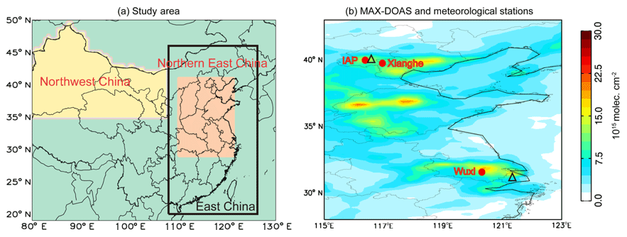
Figure 1(a) The three study areas include northern East China, northwest China, and East China. (b) MAX-DOAS measurement sites (red dots) and corresponding meteorological stations (black triangle) overlaid on POMINO v1.1 NO2 VCDs in August 2012.
The selection of CRF threshold influences the validity of pixels. The effective CRF in DOMINO implicitly includes the influence of aerosols. In POMINO, the aerosol contribution is separated from that of the clouds, resulting in a lower CRF than for DOMINO. The CRF differs insignificantly between POMINO and POMINO v1.1 because the same AOD and other non-aerosol ancillary parameters are used in the retrieval process. Using the CRF from POMINO instead of DOMINO or QA4ECV for cloud screening means that the number of valid pixels in DOMINO increases by about 25 %, particularly because many more pixels with high pollutant (aerosol and NO2) loadings are now included. This potentially reduces the sampling bias (Lin et al., 2014b, 2015), and the ensemble of pixels now includes scenes with high “aerosol radiative fractions”. Further research is needed to fully understand how much these high-aerosol scenes may be subject to the same screening issues as the cloudy scenes. Nevertheless, the limited evidence here and in Lin et al. (2014b, 2015) suggests that including these high-aerosol scenes does not affect the accuracy of NO2 retrieval.
Table 1MAX-DOAS measurement sites and corresponding meteorological stations.
2.4 MAX-DOAS data
We use MAX-DOAS measurements at three suburban or urban sites in East China, including one urban site at the Institute of Atmospheric Physics (IAP) in Beijing (116.38∘ E, 39.38∘ N), one suburban site in Xianghe County (116.96∘ E, 39.75∘ N) to the south of Beijing, and one urban site in Wuxi City (120.31∘ E, 31.57∘ N) in the Yangtze River Delta (YRD). Figure 1 shows the locations of these sites overlaid with POMINO v1.1 NO2 VCDs in August 2012. Table 1 summarizes the information of MAX-DOAS measurements.
The instruments in IAP and in Xianghe were designed at BIRA-IASB (Clémer et al., 2010). Such an instrument is a dual-channel system composed of two thermally regulated grating spectrometers, covering the ultraviolet (300–390 nm) and visible (400–720 nm) wavelengths. It measures scattered sunlight every 15 min at nine elevation angles: 2, 4, 6, 8, 10, 12, 15, 30, and 90∘. The telescope of the instrument is pointed to the north. The data are analyzed following Hendrick et al. (2014). The Xianghe suburban site is influenced by pollution from the surrounding major cities like Beijing and Tianjin. At Xianghe, MAX-DOAS data have been continuously available since early 2011, and data in 2012 are used here for comparison with OMI products. At IAP, MAX-DOAS data are available in 2008 and 2009 (Table 1); thus for comparison purposes we process OMI products to match the MAX-DOAS times.
Located on the roof of an 11-story building, the instrument at Wuxi was developed by the Anhui Institute of Optics and Fine Mechanics (AIOFM) (Wang et al., 2015, 2017a). Its telescope is pointed to the north and records at five elevation angles (5, 10, 20, 30, and 90∘). Wuxi is a typical urban site affected by heavy NOx and aerosol pollution. The measurements used here are analyzed in Wang et al. (2017a). Data are available in 2012 for comparison with OMI products.
When comparing the four OMI products against MAX-DOAS observations, temporal and spatial inconsistency in sampling is inevitable. The spatial inconsistency, together with the substantial horizontal inhomogeneity in NO2, might be more important than the influence of temporal inconsistency (Wang et al., 2017b). The influence of the horizontal inhomogeneity was suggested to be about 10 %–30 % for MAX-DOAS measurements in Beijing (Ma et al., 2013; Lin et al., 2014b) and 10 %–15 % for less polluted locations like Tai'an, Mangshan, and Rudong (Irie et al., 2012). Following previous studies, we average MAX-DOAS data within 1 h of the OMI overpass time, and we select OMI pixels within 25 km of a MAX-DOAS site whose viewing zenith angle is below 30∘. To exclude local pollution events near the MAX-DOAS site (such as the abrupt increase in NO2 caused by the pass of consequent vehicles during a very short period), the standard deviation of MAX-DOAS data within 1 h should not exceed 20 % of their mean value (Lin et al., 2014b). We elect not to spatially average the OMI pixels because they can reflect the spatial variability in NO2 and aerosols.
We further exclude MAX-DOAS data in cloudy conditions, as clouds can cause large uncertainties in MAX-DOAS and OMI data. To find the actual cloudy days, we use MODIS/Aqua cloud fraction data, MODIS/Aqua level 3 corrected reflectance (true color) data at 1∘ × 1∘ resolution, and current weather data observed from the nearest ground meteorological station (indicated by the black triangles in Fig. 1b). Since there is only one meteorological station available near the Beijing area, it is used for both IAP and Xianghe MAX-DOAS sites. We first use MODIS/Aqua corrected reflectance (true color) to distinguish clouds from haze. For cloudy days determined by the reflectance checking, we examine both the MODIS/Aqua cloud fraction data and the meteorological station cloud records, considering that MODIS/Aqua cloud fraction data may be missing or have a too coarse of a horizontal resolution to accurately interpret the cloud conditions at the MAX-DOAS site. We exclude MAX-DOAS NO2 data if the MODIS/Aqua cloud fraction is larger than 60 % and the meteorological station reports a “broken” (cloud fraction ranges from five-eighths to seven-eighths) or “overcast” (full cloud cover) sky. For the three MAX-DOAS sites together, this leads to 49 days with valid data out of 64 days with pre-screening data.
We note here that using cloud fraction data from MODIS/Aqua or MAX-DOAS (for Xianghe only, see Gielen et al., 2014) alone to screen cloudy scenes may not be appropriate on heavy-haze days. For example, on 8 January 2012, MODIS/Aqua cloud fraction is about 70 %–80 % over the North China Plain and MAX-DOAS at Xianghe suggests the presence of thick clouds. However, both the meteorological station and MODIS/Aqua corrected reflectance (true color) products suggest that the North China Plain was covered by a thick layer of haze. Consequently, this day was excluded from the analysis.
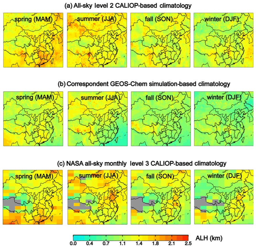
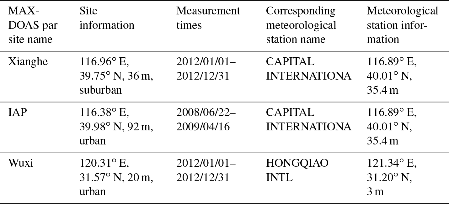
Figure 2Seasonal spatial patterns of ALH climatology at 532 nm on a 0.667∘ long × 0.50∘ lat grid based on (a) our compiled all-sky level 2 CALIOP data, (b) corresponding GEOS-Chem simulations, and (c) NASA all-sky monthly level 3 CALIOP dataset.
3.1 CALIOP monthly climatology
The aerosol layer height (ALH) is a good indicator to what extent aerosols are mixed vertically (Castellanos et al., 2015). As defined in Eq. A1 in Appendix B, the ALH is the average height of aerosols weighted by vertically resolved aerosol extinction. Figure 2a shows the spatial distribution of our CALIOP ALH climatology in each season. At most places, the ALH reaches a maximum in spring or summer and a minimum in fall or winter. The lowest ALH in fall and winter can be attributed to heavy near-surface pollution and weak vertical transport. The high values in summer are related to strong convective activities. Over the north, the high values in spring are partly associated with Asian dust events, due to high surface winds and dry soil in this season (Huang et al., 2010; Wang et al., 2010; Proestakis et al., 2018), which also affects the oceanic regions via atmospheric transport. The springtime high ALH over the south may be related to the transport of carbonaceous aerosols from Southeast Asian biomass burning (Jethva et al., 2016). Averaged over the domain, the seasonal mean ALHs are 1.48, 1.43, 1.27, and 1.18 km in spring, summer, fall, and winter.
Figure 3Regional mean ALH monthly climatology over (a) northern East China, (b) northwest China, and (c) East China. The error bars stand for 1 standard deviation for spatial variability.
Figure 3a, b further show the climatological monthly variations in ALH averaged over northern East China (the anthropogenic source region shown in orange in Fig. 1a) and northwest China (the dust source region shown in yellow in Fig. 1a). The two regions exhibit distinctive temporal variations. Over northern East China, the ALH reaches a maximum in April (∼1.53 km) and a minimum in December (∼1.14 km). Over northwest China, the ALH peaks in August (∼1.59 km) because of the strongest convection (Zhu et al., 2013), although the springtime ALH is also high.
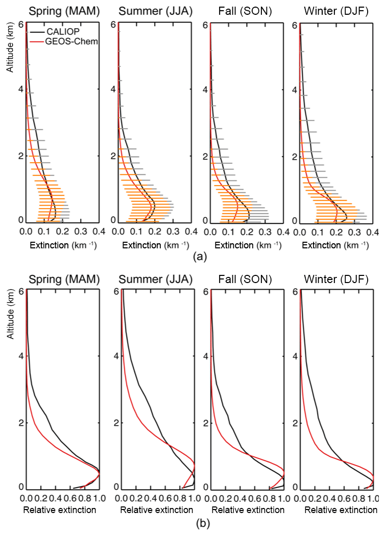
Figure 4(a) Seasonal climatological aerosol extinction profiles and (b) corresponding relative extinction profiles (normalized to maximum extinction values) in spring (MAM), summer (JJA), fall (SON), and winter (DJF) over northern East China. Model results (in red) are prior to MODIS/Aqua-based AOD adjustment. Error bars in (a) represent 1 standard deviation across all grid cells in each season.
Figure 4a shows the climatological seasonal regional average vertical profiles of aerosol extinction over northern East China. Here, the aerosol extinction increases from the ground level to a peak at about 300–600 m (season dependent), above which it decreases gradually. The height of peak extinction is lowest in winter, consistent with a stagnant atmosphere, thin mixing layer, and increased emissions (from residential and industrial sectors). The large error bars (horizontal lines in different layers, standing for 1 standard deviation) indicate strong spatiotemporal variability in aerosol extinction.
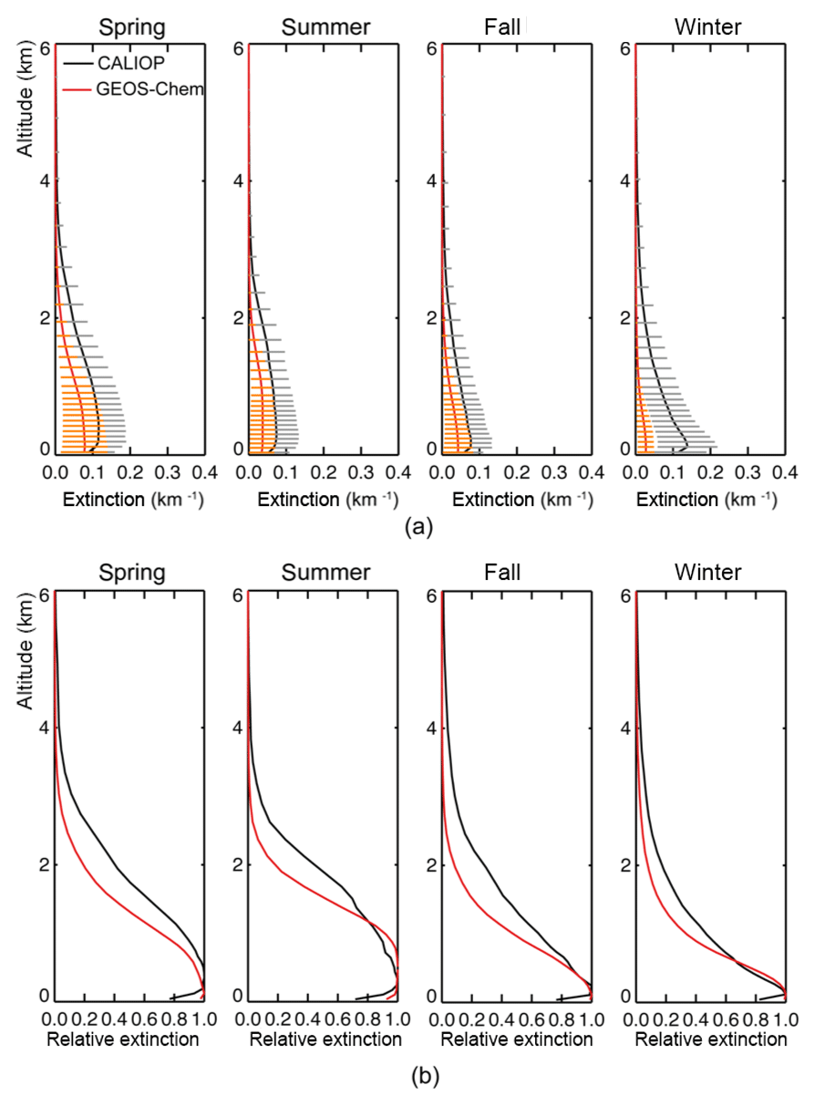
Over northwest China (Fig. 5a), the column total aerosol extinction is much smaller than that over northern East China (Fig. 4a), due to lower anthropogenic sources and dominant natural dust emissions. Vertically, the decline of extinction from the peak-extinction height to 2 km is also much more gradual than the decline over northern East China, indicating stronger lifting of surface emitted aerosols. In winter, the column total aerosol extinction is close to the high value in dusty spring, whereas the vertical gradient of extinction is strongest among the seasons. This reflects the high anthropogenic emissions in parts of northwest China, which have been rapidly increasing in the 2000s due to relatively weak emission control supplemented by growing activities of relocation of polluted industries from the eastern coastal regions (Zhao et al., 2015; Cui et al., 2016).
Overall, the spatial and seasonal variations in CALIOP aerosol vertical profiles are consistent with changes in meteorological conditions, anthropogenic sources, and natural emissions. The data will be used to evaluate and adjust GEOS-Chem simulation results in Sect. 3.2. A comparison of our CALIOP dataset with NASA's official level 3 data is presented in Appendix C.
3.2 Evaluation of GEOS-Chem aerosol extinction profiles
Figure 2b shows the spatial distribution of seasonal ALHs simulated by GEOS-Chem. The model captures the spatial and seasonal variations in CALIOP ALH (Fig. 2a) to some degree, with an underestimate by about 0.3 km on average. The spatial correlation between CALIOP (Fig. 2a) and GEOS-Chem (Fig. 2b) ALH is 0.37 in spring, 0.57 in summer, 0.40 in fall, and 0.44 in winter. The spatiotemporal consistency and underestimate are also clear from the regional mean monthly ALH data in Fig. 3 – the temporal correlation between GEOS-Chem and CALIOP ALH is 0.90 in northern East China and 0.97 in northwest China.
Figures 4a and 5a show the GEOS-Chem-simulated 2007–2015 monthly climatological vertical profiles of aerosol extinction coefficient over northern East China and northwest China, respectively. Over northern East China (Fig. 4a), the model (red line) captures the vertical distribution of CALIOP extinction (black line) below the height of 1 km, despite a slight underestimate in the magnitude of extinction and an overestimate in the peak-extinction height. From 1 to 5 km above the ground, the model substantially overestimates the rate of decline in extinction coefficient with increasing altitude. Across the seasons, GEOS-Chem underestimates the magnitude of aerosol extinction by up to 37 % (depending on the height). Over northwest China (Fig. 5a), GEOS-Chem has an underestimate in all seasons, with the largest bias by about 80 % in winter likely due to underestimated water-soluble aerosols and dust emissions (J. Wang et al., 2008; Li et al., 2016).
Since the POMINO v1.1 algorithm uses MODIS AOD to adjust model AOD, it only uses the CALIOP aerosol extinction profile shape to adjust the modeled shape (Eqs. 1 and 2). Figures 4a and 5b show the vertical shapes of aerosol extinction, averaged across all profiles in each season over northern East China and northwest China, respectively. Over northern East China (Fig. 4b), GEOS-Chem underestimates the CALIOP values above 1 km by 52 %–71 %. This underestimate leads to a lower ALH, consistent with the finding by van Donkelaar et al. (2013) and Lin et al. (2014b). Over northwest China (Fig. 5b), the model also underestimates the CALIOP values above 1 km by 50 %–62 %. These results imply the importance of correcting the modeled aerosol vertical shape prior to cloud and NO2 retrievals.
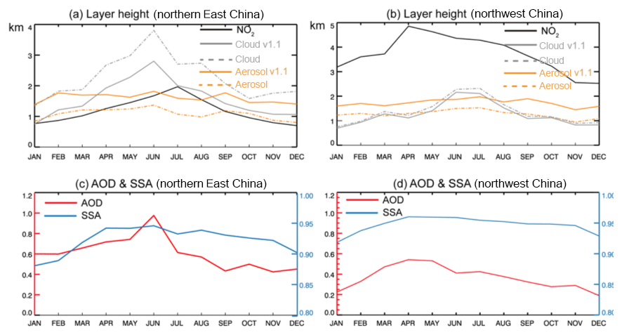
Figure 6Monthly variations in ALH, CTH, and NLH over (a) northern East China and (b) northwest China in 2012. Data are averaged across all pixels in each month and region. The grey and orange solid lines denote POMINO v1.1 results, while the corresponding dashed lines denote POMINO. (c–d) Corresponding monthly AOD and SSA.
Figure 6a, b show the monthly average ALH and cloud-top height (CTH, corresponding to cloud pressure, CP) over northern East China and northwest China in 2012. In order to discuss the CTH, only cloudy days are analyzed here, by excluding days with zero cloud fraction (CF = 0, clear-sky cases) in POMINO. Although clear sky is used sometimes in the literature to represent low cloud coverage (e.g., CF < 0.2 or CRF < 0.5; Boersma et al., 2011; Chimot et al., 2016), here it strictly means CF = 0 while cloudy sky means CF > 0. About 62.7 % of days contain non-zero fractions of clouds over northern East China, and the number is 59.1 % for northwest China. The CF changes from POMINO to POMINO v1.1 (i.e., after aerosol vertical profile adjustment) are negligible (within ±0.5 %, not shown) due to the same values of AOD and SSA used in both products. This is because overall CF is mostly driven by the continuum reflectance at 475 nm (mainly determined by AOD and surface reflectance, which remain unchanged), which is insensitive to the aerosol profile but CTH is driven by the O2–O2 SCD, which is itself impacted by ALH.
Figure 6a, b show that over the two regions, the CTH varies notably from one month to another, whereas the ALH is much more stable across the months. Over northern East China, the ALH increases by 0.52 km from POMINO (orange dashed line) to POMINO v1.1 (orange solid line) due to the CALIOP-based monthly climatological adjustment. The increase in ALH means a stronger “shielding” effect of aerosols on the O2–O2 absorbing dimer, which, in turn, results in a reduced CTH by 0.69 km on average. For POMINO over northern East China (Fig. 6a), the retrieved clouds usually extend above the aerosol layer, i.e., the CTH (grey dashed line) is much larger than the ALH (orange dashed line). Using the CALIOP climatology in POMINO v1.1 results in the ALH higher than the CTH in fall and winter. The more elevated ALH is consistent with the finding of Jethva et al. (2016) that a significant amount of absorbing aerosol resides above clouds over northern East China based on 11-year (2004–2015) OMI near-UV observations.
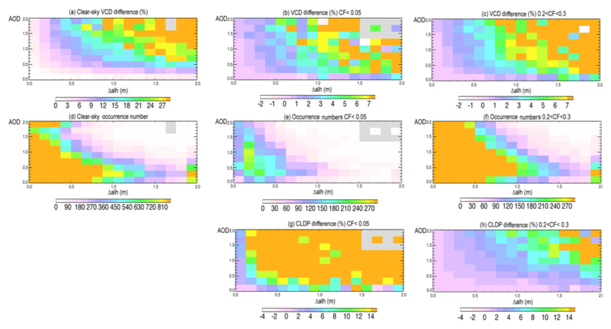
Figure 7Percentage changes in VCD from POMINO to POMINO v1.1 ([POMINO v1.1–POMINO]/POMINO) for each bin of ΔALH (bin size = 0.2 km) and AOD (bin size = 0.1) across pixels in 2012 over northern East China, for (a) cloud-free sky (CF = 0 in POMINO), (b) slightly cloudy sky, and (c) modestly cloudy sky. (d–f) The number of occurrences corresponding to (a–c). (g, h) Similar to (b, c) but for the percentage changes in cloud-top pressure (CP).
The CTH in northwest China is much lower than in northern East China (Fig. 6a versus Fig. 7b). This is because the dominant type of actual clouds is (optically thin) cirrus over western China (Wang et al., 2014), which is interpreted by the O2–O2 cloud retrieval algorithm as reduced CTH (with cloud base from the ground). The reduction in CTH from POMINO to POMINO v1.1 over northwest China is also smaller than the reduction over northern East China, albeit with a similar enhancement in ALH, due to lower aerosol loadings (Fig. 6c versus Fig. 6d).
Figure 7g, h present the relative change in CP from POMINO to POMINO v1.1 as a function of AOD (binned at an interval of 0.1) and changes in ALH from POMINO to POMINO v1.1 (ΔALH, binned every 0.2 km) across all pixels in 2012 over northern East China. Results are separated for low cloud fraction (CF < 0.05 in POMINO, Fig. 7g) and modest cloud fraction (0.2 < CF < 0.3, Fig. 7h). The median of the CP changes for pixels within each AOD and ΔALH bin is shown. Figure 7e, f present the corresponding numbers of occurrence under the two cloud conditions.
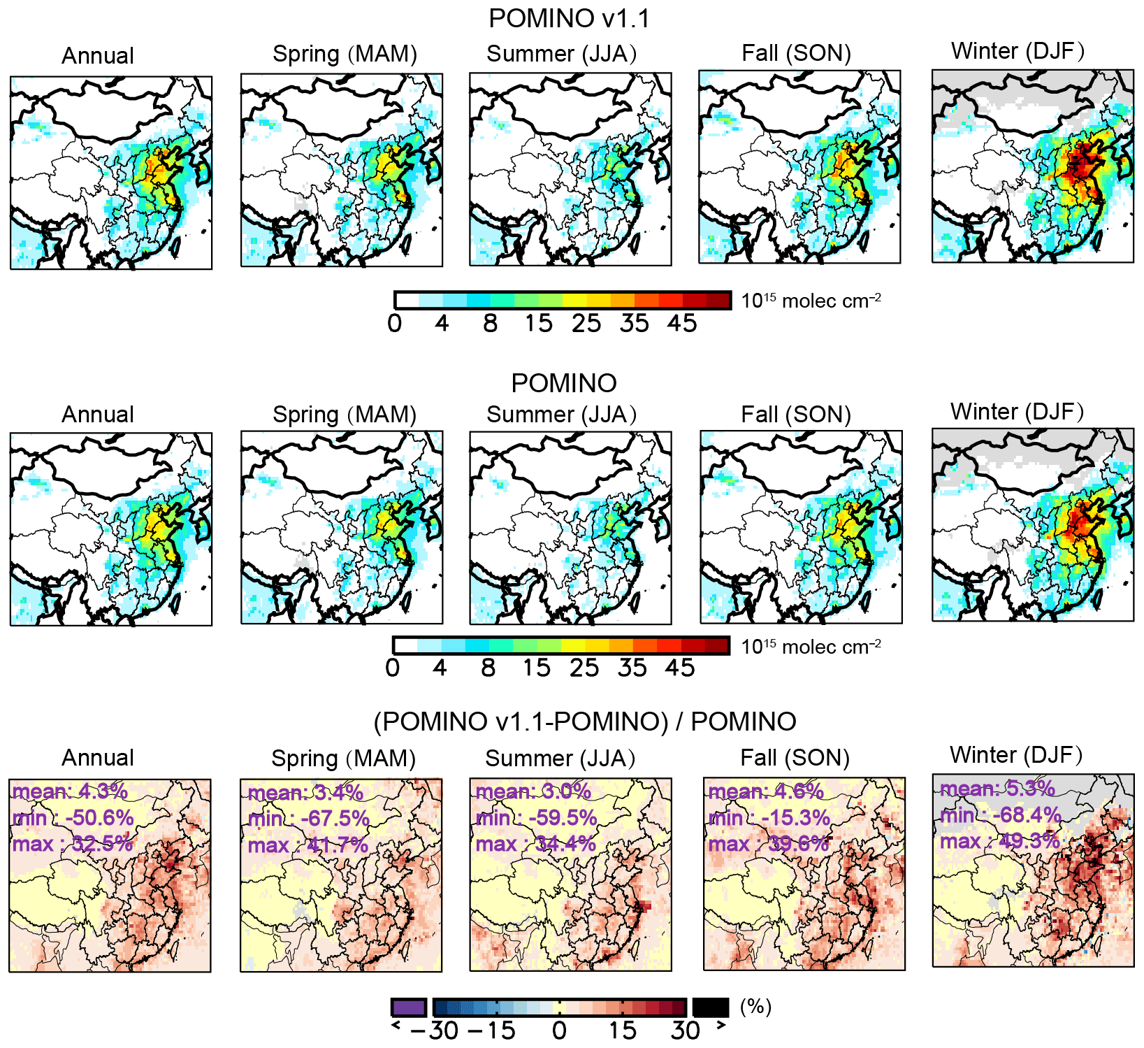
Figure 8Seasonal spatial distribution of tropospheric NO2 VCD in 2012 for (a) POMINO v1.1, (b) POMINO, and (c) their relative difference.
Figure 7 shows that over northern East China, the increase in ALH is typically within 0.6 km for the case of CF < 0.05 (Fig. 7e), and the corresponding increase in CP is within 6 % (Fig. 7g). In this case, the average CTH (2.95 km in POMINO versus 1.58 km in POMINO v1.1) becomes much lower than the average ALH (1.06 km in POMINO versus 1.98 km in POMINO v1.1). For the case with CF between 0.2 and 0.3, the increase in ALH is within 1.2 km for most scenes (Fig. 7f), which leads to a CP change of 2 % (Fig. 7h), much smaller than the CP change for CF < 0.05 (Fig. 7g). This is partly because the larger the CF is, the smaller a change in CF is required to compensate for the ΔALH in the O2–O2 cloud retrieval algorithm. Furthermore, with 0.2 < CF < 0.3, the mean value of CTH is much higher than ALH in both POMINO (2.76 km for CTH versus 1.13 km for ALH) and POMINO v1.1 (2.60 km for CTH versus 2.09 km for ALH); thus a large portion of clouds are above aerosols so that the change in CP is less sensitive to ΔALH. We find that the summertime data contribute the highest portion (36.5 %) to the occurrences for 0.2 < CF < 0.3.
For northwest China (not shown), the dependence of CP changes on AOD and ΔALH is similar to that for northern East China. In particular, the CP change is within 10 % on average for the case of CF < 0.05 and 1.5 % for the case of 0.2 < CF < 0.3.
Figure 7a presents the percentage changes in clear-sky NO2 VCD from POMINO to POMINO v1.1 as a function of binned AOD and ΔALH over northern East China. Here, clear-sky pixels are chosen based on CF = 0 in POMINO. In any AOD bin, an increase in ΔALH leads to an enhancement in NO2. And for any ΔALH, the change in VCD is greater (smaller) when AOD becomes larger (smaller), which indicates that the NO2 retrieval is more sensitive to ALH in high-aerosol-loading cases. Clearly, the change in NO2 is not a linear function of AOD and ΔALH.
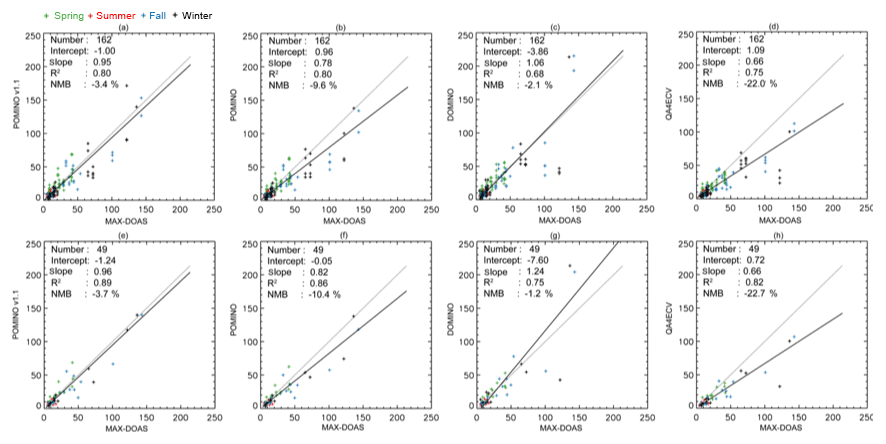
Figure 9(a–d) Scatter plot for NO2 VCDs (1015 molec. cm−2) between MAX-DOAS and each of the three OMI products. Each “+” corresponds to an OMI pixel, as several pixels may be available in a day. (e–h) Similar to (a–d) but after averaging over all OMI pixels in the same day, such that each “+” represents a day. Also shown are the statistic results from the RMA regression. The solid black line indicates the regression curve and the grey dotted line depicts the 1:1 relationship.
For cloudy scenes (Fig. 7b, c, cloud data are based on POMINO), the change in NO2 VCD is less sensitive to AOD and ΔALH. This is because the existence of clouds limits the optical effect of aerosols on tropospheric NO2. Figure 6a presents the nitrogen layer height (NLH, defined as the average height of model-simulated NO2 weighted by its volume mixing ratio in each layer) in comparison to the ALH and height of the cloud layer top (CLH) over northern East China. The figure shows that the POMINO v1.1 CTH is higher than the NLH in all months and higher than the ALH in warm months, which means there is a shielding effect on both NO2 and aerosols.
Over northwest China (not shown), the changes in clear-sky NO2 VCD are within 9 % for most cases, which are much smaller than over East China (within 18 %). This is because the NLH is much higher than the CLH and ALH (Fig. 6b) in absence of surface anthropogenic emissions.
We convert the valid pixels into monthly mean level 3 value datasets on a 0.25∘ long × 0.25∘ lat grid. Figure 8a, b compare the seasonal spatial variations in NO2 VCD in POMINO v1.1 and POMINO in 2012. In both products, NO2 peaks in winter due to the longest lifetime and highest anthropogenic emissions (Lin, 2012). NO2 also reaches a maximum over northern East China as a result of substantial anthropogenic sources. From POMINO to POMINO v1.1, the NO2 VCD increases by 3.4 % (−67.5 %–41.7 %) in spring for the domain average (range), 3.0 % (−59.5 %–34.4 %) in summer, 4.6 % (−15.3 %–39.6 %) in fall, and 5.3 % (−68.4 %–49.3 %) in winter. The NO2 change is highly dependent on the location and season. The increase over northern East China is largest in winter, wherein the positive value for ΔALH implies that elevated aerosol layers shield the NO2 absorption.
Table 2Pixel-based evaluation of OMI NO2 products with respect to MAX-DOAS for 162 pixels on 49 days.
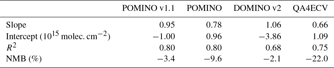
We use MAX-DOAS data, after cloud screening (Sect. 2.4), to evaluate DOMINO v2, QA4ECV, POMINO, and POMINO v1.1. The scatter plots in Fig. 9a–d compare the NO2 VCDs from 162 OMI pixels on 49 days with their MAX-DOAS counterparts. The statistical results are shown in Table 2 as well. Different colors differentiate the seasons. The high values of NO2 VCD (> 30 ×1015 molec. cm−2) occur mainly in fall (blue) and winter (black). POMINO v1.1 and POMINO capture the day-to-day variability in MAX-DOAS data, i.e., R2=0.80 for both products. The normalized mean bias (NMB) of POMINO v1.1 relative to MAX-DOAS data (−3.4 %) is smaller than the NMB of POMINO (−9.6 %). Also, the reduced major axis (RMA) regression shows that the slope for POMINO v1.1 (0.95) is closer to unity than the slope for POMINO (0.78). When all OMI pixels in a day are averaged (Fig. 9e, f), the correlation across the total of 49 days further increases for both POMINO v1.1 (R2=0.89) and POMINO (R2=0.86), whereas POMINO v1.1 still has a lower NMB (−3.7 %) and better slope (0.96) than POMINO (−10.4 % and 0.82, respectively). These results suggest that correcting aerosol vertical profiles, at least on a climatology basis, already leads to a significantly improved NO2 retrieval from OMI.
Table 3Pixel-based evaluation of OMI NO2 products with respect to MAX-DOAS for 27 pixels on 11 haze daysa.

a The haze days are determined when the ground meteorological station data and MODIS/Aqua corrected reflectance (true color) data both indicate a haze day. Averages across the pixels are as follows: AOD = 1.13 (median = 1.10), SSA = 0.90 (0.91), MAX-DOAS NO2 molec. cm−2, and CF = 0.06 (0.03).
Figure 9 shows that DOMINO v2 is correlated with MAX-DOAS (R2=0.68 in Fig. 9c and 0.75 in Fig. 9g) but not as strong as POMINO and POMINO v1.1 for all days. The discrepancy between DOMINO v2 and MAX-DOAS is particularly large for very high NO2 values (> 70×1015 molec. cm−2). The R2 for QA4ECV (0.75 in Fig. 9d and 0.82 in Fig. 9h) is slightly better than DOMINO, but the NMB is higher (−22.0 % and −22.7 %) and the slope drops to 0.66. These results are consistent with the finding of Lin et al. (2014b, 2015) that explicitly including aerosol optical effects improves the NO2 retrieval.
Table 4Evaluation of OMI NO2 products with respect to MAX-DOAS of 36 pixels on 18 cloud-free daysa.
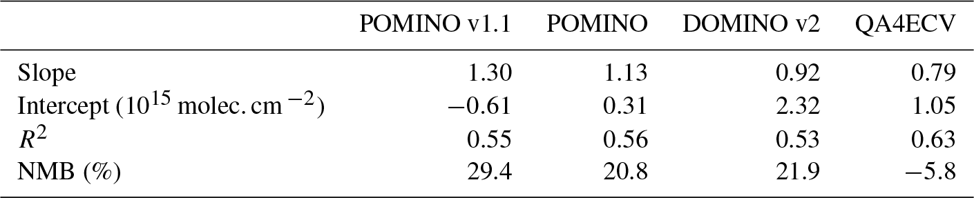
a CF = 0 in POMINO product. Averages across the pixels are as follows: AOD = 0.60 (median = 0.47), SSA = 0.90 (0.91), and MAX-DOAS NO2 molec. cm−2.
Table 3 further shows the comparison statistics for 11 haze days. The haze days are determined when both the ground meteorological station data and MODIS/Aqua corrected reflectance (true color) data indicate a haze day. The table also lists AOD, SSA, CF, and MAX-DOAS NO2 VCD as averaged over all haze days. A large amount of absorbing aerosol occurs on these haze days (AOD = 1.13, SSA = 0.90). The average MAX-DOAS NO2 VCD reaches 51.9×10¹⁵ molec. cm−2. Among the four satellite products, POMINO v1.1 has the highest R2 (0.76) and the lowest bias (4.4 %) with respect to MAX-DOAS, whereas DOMINO v2 and QA4ECV reproduce the variability to a limited extent (R2=0.38 and 0.34, respectively). This is consistent with the previous finding that the accuracy of DOMINO v2 is reduced for polluted, aerosol-loaded scenes (Boersma et al., 2011; Kanaya et al., 2014; Lin et al., 2014b; Chimot et al., 2016).
Table 4 shows the comparison statistics for 18 cloud-free days (CF = 0 in POMINO, and AOD = 0.60 on average). Here, POMINO v1.1, POMINO, and DOMINO v2 do not show large differences in R2 (0.53–0.56) and NMB (20.8 %–29.4 %) with respect to MAX-DOAS. QA4ECV has a higher R2 (0.63) and a lower NMB (−5.8 %), presumably reflecting the improvements in this (EU) consortium approach, at least in mostly cloud-free situations. However, the R2 values for POMINO and POMINO v1.1 are much smaller than the R2 values on haze days, whereas the opposite changes are true for DOMINO v2 and QA4ECV. Thus, for this limited set of data, the changes from DOMINO v2 and QA4ECV to POMINO and POMINO v1.1 mainly reflect the improved aerosol treatment in hazy scenes. Further research may use additional MAX-DOAS datasets to evaluate the satellite products more systematically.
This paper improves upon our previous POMINO algorithm (Lin et al., 2015) to retrieve the tropospheric NO2 VCDs from OMI by compiling a 9-year (2007–2015) CALIOP monthly climatology of aerosol vertical extinction profiles to adjust GEOS-Chem aerosol profiles used in the NO2 retrieval process. The improved algorithm is referred to as POMINO v1.1. Compared to monthly climatological CALIOP data over China, GEOS-Chem simulations tend to underestimate the aerosol extinction above 1 km, as characterized by an underestimate in ALH by 300–600 m (seasonal and location dependent). Such a bias is corrected in POMINO v1.1 by dividing, for any month and grid cell, the CALIOP monthly climatological profile by the model climatological profile to obtain a scaling profile and then applying the scaling profile to model data on all days of that month in all years.
The aerosol extinction profile correction leads to an insignificant change in CF from POMINO to POMINO v1.1 since the AOD and surface reflectance are unchanged. In contrast, the correction results in a notable increase in CP (i.e., a decrease in CTH), due to lifting of aerosol layers. The CP changes are generally within 6 % for scenes with a low cloud fraction (CF < 0.05 in POMINO) and within 2 % for scenes with a modest cloud fraction (0.2 < CF < 0.3 in POMINO).
The NO2 VCDs increase from POMINO to POMINO v1.1 in most cases due to lifting of aerosol layers that enhances the shielding of NO2 absorption. The NO2 VCD increases by 3.4 % (−67.5 %–41.7 %) in spring for the domain average (range), 3.0 % (−59.5 %–34.4 %) in summer, 4.6 % (−15.3 %–39.6 %) in fall, and 5.3 % (−68.4 %–49.3 %) in winter. The NO2 changes are highly season and location dependent and are most significant for wintertime in northern East China.
Further comparisons with independent MAX-DOAS NO2 VCD data for 162 OMI pixels on 49 days show good performance of both POMINO v1.1 and POMINO in capturing the day-to-day variation in NO2 (R2=0.80, n=162), compared to DOMINO v2 (R2=0.67) and the new QA4ECV product (R2=0.75). The NMB is smaller in POMINO v1.1 (−3.4 %) than in POMINO (−9.6 %), with a slightly better slope (0.804 versus 0.784). On hazy days with high aerosol loadings (AOD = 1.13 on average), POMINO v1.1 has the highest R2 (0.76) and the lowest bias (4.4 %) whereas DOMINO and QA4ECV have difficulty in reproducing the day-to-day variability in MAX-DOAS NO2 measurements (R2=0.38 and 0.34, respectively). The four products show small differences in R2 on clear-sky days (CF = 0 in POMINO, AOD = 0.60 on average), among which QA4ECV shows the highest R2 (0.63) and lowest NMB (−5.8 %), presumably reflecting the improvements in less polluted places such as Europe and the US. Thus the explicit aerosol treatment (in POMINO and POMINO v1.1) and the aerosol vertical profile correction (in POMINO v1.1) improve the NO2 retrieval, especially in hazy cases.
The POMINO v1.1 algorithm is a core step towards our next public release of data product, POMINO v2. The v2 product will contain a few additional updates, including but not limited to using MODIS Collection 6 merged 10 km level 2 AOD data that combine the Dark Target (Levy et al., 2013) and Deep Blue (Sayer et al., 2014) products, as well as MODIS MCD43C2 Collection 6 daily BRDF data. Meanwhile, the POMINO algorithm framework is being applied to the recently launched TROPOMI instrument that provides NO2 information at a much higher spatial resolution (3.5×7 km2). A modified algorithm can also be used to retrieve sulfur dioxide, formaldehyde, and other trace gases from TROPOMI, for which purposes our algorithm will be available to the community on a collaborative basis. Future research can correct the SSA and NO2 vertical profile to further improve the retrieval algorithm and can use more comprehensive independent data to evaluate the resulting satellite products.
DOMINO v2 NO2 Level-2 data are available at http://www.temis.nl/airpollution/no2col/data/omi/data_v2/ (European Space Agency, 2018); QA4ECV NO2 Level-2 data at http://www.temis.nl/qa4ecv/no2col/data/omi/v1/ (European Space Agency, 2018); and POMINO v2 NO2 Level-2 and Level-3 data at https://www.amazon.com/clouddrive/share/zyC4mNEyRfRk0IX114sR51lWTMpcP1d4SwLVrW55iFG/folder/S7IR7WSLSPikdLT_jsNX8g?_encoding=UTF8&*Version*=1&*entries*=0&mgh=1 (ACM group at Peking University, 2018). POMINO NO2 v1.1 Level-2 data are available upon request. MODIS C5.1 AOD Level-2 data https://doi.org/10.1029/2006JD007815 (NASA Goddard Space Flight, 2018); CALIOP v3 Level-2 aerosol extinction profile data https://doi.org/10.1175/2010BAMS3009.1 (NASA Goddard Space Flight, 2018); CALIOP Level-3 aerosol extinction profile data https://doi.org/10.5194/acp-13-3345-2013 (NASA Goddard Space Flight, 2018). MAX-DOAS data are available through contact with the various data owners.
The QA4ECV NO2 product (http://www.qa4ecv.eu/, last access: May 2018) builds on a (EU) consortium approach to retrieve NO2 from GOME, SCIAMACHY, GOME-2, and OMI. The main contributions are provided by BIRA-IASB, the University of Bremen (IUP), MPIC, KNMI, and Wageningen University. Uncertainties in spectral fitting for NO2 SCDs and in AMF calculations were evaluated by Zara et al. (2018) and Lorente et al. (2017), respectively. QA4ECV contains improved SCD NO2 data (Zara et al., 2018). Our test suggests that using the QA4ECV SCD data instead of DOMINO SCD data would reduce the underestimate against MAX-DOAS VCD data from 3.7 % to 0.2 %, a relatively minor improvement. Lorente et al. (2017) showed that across the above algorithms, there is a structural uncertainty by 42 % in the NO2 AMF calculation over polluted areas. By comparing to our POMINO product, Lorente et al. also showed that the choice of aerosol correction may introduce an additional uncertainty by up to 50 % for situations with high polluted cases, consistent with Lin et al. (2014b, 2015) and the findings here. For a complete description of the QA4ECV algorithm improvements, and quality assurance, please see Boersma et al. (2018).
Table A1Number of CALIOP observations in a grid cell (0.667∘ × 0.5∘).
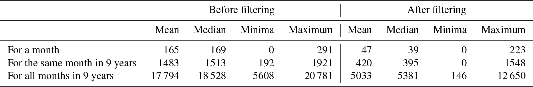
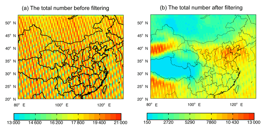
Figure A1The total number of CALIOP level 2 aerosol extinction profiles at 532 nm used to derive our climatological (2007–2015) dataset on a 0.667∘ long × 0.5∘ lat grid (a) before and (b) after filtering.
We use the all-sky level 2 CALIOP data to construct the level 3 monthly climatology. We choose the all-sky product instead of clear-sky data since previous studies indicate that the climatological aerosol extinction profiles are affected insignificantly by the presence of clouds (Koffi et al., 2012; Winker et al., 2013). As we use this climatological data to adjust GEOS-Chem results, choosing all-sky data improves consistency with the model simulation when doing the daily correction.
To select valid pixels, we follow the data quality criteria by Winker et al. (2013) and Amiridis et al. (2015). Only the pixels with cloud–aerosol discrimination (CAD) scores between −20 and −100 with an extinction quality control (QC) flag valued at 0, 1, 18, and 16 are selected. We further discard samples with an extinction uncertainty of 99.9 km−1, which is indicative of unreliable retrieval. We only accept extinction values falling in the range from 0.0 to 1.25, according to CALIOP observation thresholds. Previous studies showed that weakly scattering edges of icy clouds are sometimes misclassified as aerosols (Winker et al., 2013). To eliminate contamination from icy clouds we exclude the aerosol layers above the cloud layer (with layer-top temperature below 0∘) when both of them are above 4 km (Winker et al., 2013).
After the pixel-based screening, we aggregate the CALIOP data at the model grid (0.667∘ long × 0.5∘ lat) and vertical resolution (47 layers, with 36 layers or so in the troposphere). For each grid cell, we choose the CALIOP pixels within 1.5∘ of the grid cell center. CALIOP level 2 data are always presented at the fixed 399 altitudes above sea level. To account for the difference in surface elevation between a CALIOP pixel and the respective model grid cell, we convert the altitude of the pixel to a height above the ground, by using the surface elevation data provided in CALIOP. We then horizontally and vertically average the profiles of all pixels within one model grid cell and layer. We do the regridding day by day for all grid cells to ensure that GEOS-Chem and CALIOP extinction profiles are coincident spatially and temporally. Finally, we compile a monthly climatological dataset by averaging over 2007–2015.
Figure A1 shows the number of aerosol extinction profiles in each grid cell and months that are used to compile the CALIOP climatology, both before and after data screening. Table A1 presents additional information on monthly and yearly bases. On average, there are 165 and 47 aerosol extinction profiles per month per grid cell before and after screening, respectively. In the final 9-year monthly climatology, each grid cell has about 420 aerosol extinction profiles on average, about 28 % of the prior-screening profiles. Figure A1 shows that the number of valid profiles decreases sharply over the Tibet Plateau and at higher latitudes (> 43∘ N) due to complex terrain and icy/snowy ground.
As discussed above, we choose the CALIOP pixels within 1.5∘ of a grid cell center. We test this choice by examining the ALH produced for that grid cell. The ALH is defined as the extinction-weighted height of aerosols (see Eq. A1, where n denotes the number of tropospheric layers, εi the aerosol extinction at layer i, and Hi the layer center height above the ground). We find that choosing pixels within 1.0∘ of a grid cell center leads to a noisier horizontal distribution of ALH, owing to the small footprint of CALIOP. Conversely, choosing 2.0∘ leads to a too smooth spatial gradient of ALH with local characteristics of aerosol vertical distributions largely lost. We thus decide that 1.5∘ is a good balance between noise and smoothness.
Certain grid cells do not contain sufficient valid observations for some months of the climatological dataset. We fill in missing monthly values of a grid cell using valid data in the surrounding grid cells (within ∼100 km). If the 25 grid cells do not have enough valid data, we use those in the surrounding grid cells (within ∼150 km). A similar procedure is used by Lin et al. (2014b, 2015) to fill in missing values in the gridded MODIS AOD dataset.
For each grid cell in each month, we further correct singular values in the vertical profile. In a month, if a grid cell i has an ALH outside mean ± 1σ of its surrounding 25 or 49 grid cells, we select i's surrounding grid cell j whose ALH is the median of i's surrounding grid cells, and we use j's profile to replace i's. Whether 25 or 49 surrounding grid cells are chosen depends on the number of valid pixels shown in Fig. A1b. If the number of valid pixels in i is below mean–1σ of all grid cells in the whole domain, which is often the case for Tibetan grid cells, we use i's surrounding 49 grid cells; otherwise we use i's surrounding 25 grid cells.
We compare our gridded climatological profiles to NASA CALIOP version 3 level 3 all-sky monthly profiles at 532 nm (Winker et al., 2013). The NASA level 3 data have a horizontal resolution of 2∘ lat × 5∘ long and a vertical resolution of 60 m (from −0.5 to 12 km above sea level). We combine NASA monthly data over 2007–2015 to construct a monthly climatology for comparison with our own compilation. We only choose aerosol extinction data in the troposphere with an error less than 0.15 (the valid range given in the CALIOP dataset). If the number of valid monthly profiles in a grid cell is less than five (i.e., for the same month in 5 out of the 9 years), then we exclude data in that grid cell; see the dark gray grid cells in Fig. 2c.
Several methodological differences exist between generating our and NASA CALIOP datasets. First, the two datasets have different horizontal resolutions. Also, we sample all valid CALIOP pixels within 1.5∘ of a grid cell center, whereas the NASA dataset samples all valid pixels within a grid cell. In addition, our CALIOP dataset involves several steps of horizontal interpolation, for purposes of subsequent cloud and NO2 retrievals, which is not performed in the NASA dataset. In addition, we match CALIOP data vertically to the GEOS-Chem vertical resolution, whereas the NASA dataset maintains the original resolution.
Figure 2c shows the spatial distribution of ALH in all seasons based on NASA CALIOP level 3 all-sky monthly climatology. The horizontal resolution of NASA data is much coarser than ours, and NASA data are largely missing over the southwest with complex terrains. We choose to focus on the comparison over East China (the black box in Fig. 1a). Over East China, the two climatology datasets generally exhibit similar spatial patterns of ALH in all seasons (Fig. 2a, c). The NASA dataset suggests higher ALHs than ours over East China, especially in summer, due mainly to differences in the sampling and regridding processes. Figure 3c further compares the monthly variation in ALH between our (black line with error bars) and NASA (blue filled triangles) datasets averaged over East China. The two datasets are consistent in almost all months, indicating that their regional differences are largely smoothed out by spatial averaging.
ML and JL conceived the research. ML, JL and KF designed the research. ML performed the research. GP, YW, ThW, PX, MVR, FH, PW and TiW provided MAX-DOAS data. HE and JC contributed to CALIOP data processing. ML, JL and KF analyzed the results with comments from YY, LC and RN. ML, JL and KF wrote the paper with input from all authors.
The authors declare that they have no conflict of interest.
This research is supported by the National Natural Science Foundation of
China (41775115), the 973 program (2014CB441303), the Chinese Scholarship
Council, and the EU FP7 QA4ECV project (grant no. 607405).
Edited by: Diego Loyola
Reviewed by: two
anonymous referees
Acarreta, J. R., De Haan, J. F., and Stammes, P.: Cloud pressure retrieval using the O2-O2 absorption band at 477 nm, J. Geophys. Res., 109, D05204, https://doi.org/10.1029/2003JD003915, 2004.
ACM group at Peking University: POMINO v2 NO2 Level-2 and Level-3 data, available at: https://www.amazon.com/clouddrive/share/zyC4mNEyRfRk0IX114sR51lWTMpcP1d4SwLVrW55iFG/folder/S7IR7WSLSPikdLT_jsNX8g?_encoding=UTF8&*Version*=1&*entries*=0&mgh=1, last access: 20 December 2018.
Amiridis, V., Marinou, E., Tsekeri, A., Wandinger, U., Schwarz, A., Giannakaki, E., Mamouri, R., Kokkalis, P., Binietoglou, I., Solomos, S., Herekakis, T., Kazadzis, S., Gerasopoulos, E., Proestakis, E., Kottas, M., Balis, D., Papayannis, A., Kontoes, C., Kourtidis, K., Papagiannopoulos, N., Mona, L., Pappalardo, G., Le Rille, O., and Ansmann, A.: LIVAS: a 3-D multi-wavelength aerosol/cloud database based on CALIPSO and EARLINET, Atmos. Chem. Phys., 15, 7127–7153, https://doi.org/10.5194/acp-15-7127-2015, 2015.
Belmonte Rivas, M., Veefkind, P., Boersma, F., Levelt, P., Eskes, H., and Gille, J.: Intercomparison of daytime stratospheric NO2 satellite retrievals and model simulations, Atmos. Meas. Tech., 7, 2203–2225, https://doi.org/10.5194/amt-7-2203-2014, 2014.
Boersma, K. F., Bucsela, E. J., Brinksma, E. J., and Gleason, J. F.: NO2, in: OMI Algorithm Theoretical Basis Document, vol. 4, OMI Trace Gas Algorithms, ATB-OMI-04, Version 2.0, edited by: Chance, K., NASA Distrib. Active Archive Cent., Greenbelt, Md., August, 13–36, 2002.
Boersma, K. F., Eskes, H. J., and Brinksma, E. J.: Error analysis for tropospheric NO2 retrieval from space, J. Geophys. Res.-Atmos., 109, D04311, https://doi.org/10.1029/2003JD003962, 2004.
Boersma, K. F., Eskes, H. J., Veefkind, J. P., Brinksma, E. J., van der A, R. J., Sneep, M., van den Oord, G. H. J., Levelt, P. F., Stammes, P., Gleason, J. F., and Bucsela, E. J.: Near-real time retrieval of tropospheric NO2 from OMI, Atmos. Chem. Phys., 7, 2103–2118, https://doi.org/10.5194/acp-7-2103-2007, 2007.
Boersma, K. F., Eskes, H. J., Dirksen, R. J., van der A, R. J., Veefkind, J. P., Stammes, P., Huijnen, V., Kleipool, Q. L., Sneep, M., Claas, J., Leitão, J., Richter, A., Zhou, Y., and Brunner, D.: An improved tropospheric NO2 column retrieval algorithm for the Ozone Monitoring Instrument, Atmos. Meas. Tech., 4, 1905–1928, https://doi.org/10.5194/amt-4-1905-2011, 2011.
Boersma, K. F., Eskes, H. J., Richter, A., De Smedt, I., Lorente, A., Beirle, S., van Geffen, J. H. G. M., Zara, M., Peters, E., Van Roozendael, M., Wagner, T., Maasakkers, J. D., van der A, R. J., Nightingale, J., De Rudder, A., Irie, H., Pinardi, G., Lambert, J.-C., and Compernolle, S.: Improving algorithms and uncertainty estimates for satellite NO2 retrievals: Results from the Quality Assurance for Essential Climate Variables (QA4ECV) project, Atmos. Meas. Tech. Discuss., https://doi.org/10.5194/amt-2018-200, in review, 2018.
Bucsela, E. J., Celarier, E. A., Wenig, M. O., Gleason, J. F., Veefkind, J. P., Boersma, K. F., and Brinksma, E. J.: Algorithm for NO2 vertical column retrieval from the ozone monitoring instrument, IEEE T. Geosci. Remote, 44, 1245–1258, https://doi.org/10.1109/TGRS.2005.863715, 2006.
Bucsela, E. J., Krotkov, N. A., Celarier, E. A., Lamsal, L. N., Swartz, W. H., Bhartia, P. K., Boersma, K. F., Veefkind, J. P., Gleason, J. F., and Pickering, K. E.: A new stratospheric and tropospheric NO2 retrieval algorithm for nadir-viewing satellite instruments: applications to OMI, Atmos. Meas. Tech., 6, 2607–2626, https://doi.org/10.5194/amt-6-2607-2013, 2013.
Castellanos, P., Boersma, K. F., and van der Werf, G. R.: Satellite observations indicate substantial spatiotemporal variability in biomass burning NOx emission factors for South America, Atmos. Chem. Phys., 14, 3929–3943, https://doi.org/10.5194/acp-14-3929-2014, 2014.
Castellanos, P., Boersma, K. F., Torres, O., and de Haan, J. F.: OMI tropospheric NO2 air mass factors over South America: effects of biomass burning aerosols, Atmos. Meas. Tech., 8, 3831–3849, https://doi.org/10.5194/amt-8-3831-2015, 2015.
Chazette, P., Raut, J.-C., Dulac, F., Berthier, S., Kim, S.-W., Royer, P., Sanak, J., Loaëc, S., and Grigaut-Desbrosses, H.: Simultaneous observations of lower tropospheric continental aerosols with a ground-based, an airborne, and the spaceborne CALIOP lidar system, J. Geophys. Res., 115, D00H31, https://doi.org/10.1029/2009JD012341, 2010.
Chimot, J., Vlemmix, T., Veefkind, J. P., de Haan, J. F., and Levelt, P. F.: Impact of aerosols on the OMI tropospheric NO2 retrievals over industrialized regions: how accurate is the aerosol correction of cloud-free scenes via a simple cloud model?, Atmos. Meas. Tech., 9, 359–382, https://doi.org/10.5194/amt-9-359-2016, 2016.
Clémer, K., Van Roozendael, M., Fayt, C., Hendrick, F., Hermans, C., Pinardi, G., Spurr, R., Wang, P., and De Mazière, M.: Multiple wavelength retrieval of tropospheric aerosol optical properties from MAXDOAS measurements in Beijing, Atmos. Meas. Tech., 3, 863–878, https://doi.org/10.5194/amt-3-863-2010, 2010.
Cui, Y., Lin, J., Song, C., Liu, M., Yan, Y., Xu, Y., and Huang, B.: Rapid growth in nitrogen dioxide pollution over Western China, 2005–2013, Atmos. Chem. Phys., 16, 6207–6221, https://doi.org/10.5194/acp-16-6207-2016, 2016.
Dirksen, R. J., Boersma, K. F., Eskes, H. J., Ionov, D. V., Bucsela, E. J., Levelt, P. F., and Kelder, H. M.: Evaluation of stratospheric NO2 retrieved from the Ozone Monitoring Instrument: Intercomparison, diurnal cycle, and trending, J. Geophys. Res., 116, D08305, https://doi.org/10.1029/2010JD014943, 2011.
European Space Agency: DOMINO v2 NO2 Level-2 data, available at: http://www.temis.nl/airpollution/no2col/data/omi/data_v2/, last access: 20 December 2018.
European Space Agency: QA4ECV NO2 Level-2 data, available at: http://www.temis.nl/qa4ecv/no2col/data/omi/v1/, last access: 20 December 2018.
Gielen, C., Van Roozendael, M., Hendrick, F., Pinardi, G., Vlemmix, T., De Bock, V., De Backer, H., Fayt, C., Hermans, C., Gillotay, D., and Wang, P.: A simple and versatile cloud-screening method for MAX-DOAS retrievals, Atmos. Meas. Tech., 7, 3509–3527, https://doi.org/10.5194/amt-7-3509-2014, 2014.
Hendrick, F., Müller, J.-F., Clémer, K., Wang, P., De Mazière, M., Fayt, C., Gielen, C., Hermans, C., Ma, J. Z., Pinardi, G., Stavrakou, T., Vlemmix, T., and Van Roozendael, M.: Four years of ground-based MAX-DOAS observations of HONO and NO2 in the Beijing area, Atmos. Chem. Phys., 14, 765–781, https://doi.org/10.5194/acp-14-765-2014, 2014.
Huang, Z., Huang, J., Bi, J., Wang, G., Wang, W., Fu, Q., Li, Z., Tsay, S.-C., and Shi, J.: Dust aerosol vertical structure measurements using three MPL lidars during 2008 China-U.S. joint dust field experiment, J. Geophys. Res.-Atmos., 115, D00K15, https://doi.org/10.1029/2009JD013273, 2010.
Irie, H., Boersma, K. F., Kanaya, Y., Takashima, H., Pan, X., and Wang, Z. F.: Quantitative bias estimates for tropospheric NO2 columns retrieved from SCIAMACHY, OMI, and GOME-2 using a common standard for East Asia, Atmos. Meas. Tech., 5, 2403–2411, https://doi.org/10.5194/amt-5-2403-2012, 2012.
Jethva, H., Torres, O., and Changwoo, A.: A ten-year global record of absorbing aerosols above clouds from OMI's near-UV observations, Proc. SPIE 9876, Remote Sensing of the Atmosphere, Clouds, and Precipitation VI, 9876, 1A, https://doi.org/10.1117/12.2225765, 2016.
Johnson, M. S., Meskhidze, N., and Praju Kiliyanpilakkil, V.: A global comparison of GEOS-Chem-predicted and remotely-sensed mineral dust aerosol optical depth and extinction profiles, J. Adv. Model. Earth Sy., 4, M07001, https://doi.org/10.1029/2011MS000109, 2012.
Kacenelenbogen, M., Redemann, J., Vaughan, M. A., Omar, A. H., Russell, P. B., Burton, S., Rogers, R. R., Ferrare, R. A., and Hostetler, C. A.: An evaluation of CALIOP/CALIPSO's aerosol-above-cloud detection and retrieval capability over North America, J. Geophys. Res.-Atmos., 119, 230–244, https://doi.org/10.1002/2013JD020178, 2014.
Kanaya, Y., Irie, H., Takashima, H., Iwabuchi, H., Akimoto, H., Sudo, K., Gu, M., Chong, J., Kim, Y. J., Lee, H., Li, A., Si, F., Xu, J., Xie, P.-H., Liu, W.-Q., Dzhola, A., Postylyakov, O., Ivanov, V., Grechko, E., Terpugova, S., and Panchenko, M.: Long-term MAX-DOAS network observations of NO2 in Russia and Asia (MADRAS) during the period 2007–2012: instrumentation, elucidation of climatology, and comparisons with OMI satellite observations and global model simulations, Atmos. Chem. Phys., 14, 7909–7927, https://doi.org/10.5194/acp-14-7909-2014, 2014.
Kim, S.-W., Heckel, A., Frost, G. J., Richter, A., Gleason, J., Burrows, J. P., McKeen, S., Hsie, E.-Y., Granier, C., and Trainer, M.: NO2 columns in the western United States observed from space and simulated by a regional chemistry model and their implications for NOx emissions, J. Geophys. Res., 114, D11301, https://doi.org/10.1029/2008JD011343, 2009.
Koffi, B., Schulz, M., Bréon, F.-M., Griesfeller, J., Winker, D., Balkanski, Y., Bauer, S., Berntsen, T., Chin, M., Collins, W. D., Dentener, F., Diehl, T., Easter, R., Ghan, S., Ginoux, P., Gong, S., Horowitz, L. W., Iversen, T., Kirkevåg, A., Koch, D., Krol, M., Myhre, G., Stier, P., and Takemura, T.: Application of the CALIOP layer product to evaluate the vertical distribution of aerosols estimated by global models: AeroCom phase I results, J. Geophys. Res.-Atmos., 117, D10201, https://doi.org/10.1029/2011JD016858, 2012.
Leitão, J., Richter, A., Vrekoussis, M., Kokhanovsky, A., Zhang, Q. J., Beekmann, M., and Burrows, J. P.: On the improvement of NO2 satellite retrievals – aerosol impact on the airmass factors, Atmos. Meas. Tech., 3, 475–493, https://doi.org/10.5194/amt-3-475-2010, 2010.
Lerot, C., Stavrakou, T., De Smedt, I., Müller, J.-F., and Van Roozendael, M.: Glyoxal vertical columns from GOME-2 backscattered light measurements and comparisons with a global model, Atmos. Chem. Phys., 10, 12059–12072, https://doi.org/10.5194/acp-10-12059-2010, 2010.
Levy, R. C., Mattoo, S., Munchak, L. A., Remer, L. A., Sayer, A. M., Patadia, F., and Hsu, N. C.: The Collection 6 MODIS aerosol products over land and ocean, Atmos. Meas. Tech., 6, 2989–3034, https://doi.org/10.5194/amt-6-2989-2013, 2013.
Li, S., Yu, C., Chen, L., Tao, J., Letu, H., Ge, W., Si, Y., and Liu, Y.: Inter-comparison of model-simulated and satellite-retrieved componential aerosol optical depths in China, Atmos. Environ., 141, 320–332, https://doi.org/10.1016/j.atmosenv.2016.06.075, 2016.
Lin, J., Pan, D., Davis, S. J., Zhang, Q., He, K., Wang, C., Streets, D. G., Wuebbles, D. J., and Guan, D.: China's international trade and air pollution in the United States, P. Natl. Acad. Sci. USA, 111, 1736–1741, https://doi.org/10.1073/pnas.1312860111, 2014a.
Lin, J.-T., McElroy, M. B., and Boersma, K. F.: Constraint of anthropogenic NOx emissions in China from different sectors: a new methodology using multiple satellite retrievals, Atmos. Chem. Phys., 10, 63–78, https://doi.org/10.5194/acp-10-63-2010, 2010.
Lin, J.-T.: Satellite constraint for emissions of nitrogen oxides from anthropogenic, lightning and soil sources over East China on a high-resolution grid, Atmos. Chem. Phys., 12, 2881–2898, https://doi.org/10.5194/acp-12-2881-2012, 2012.
Lin, J.-T., Martin, R. V., Boersma, K. F., Sneep, M., Stammes, P., Spurr, R., Wang, P., Van Roozendael, M., Clémer, K., and Irie, H.: Retrieving tropospheric nitrogen dioxide from the Ozone Monitoring Instrument: effects of aerosols, surface reflectance anisotropy, and vertical profile of nitrogen dioxide, Atmos. Chem. Phys., 14, 1441–1461, https://doi.org/10.5194/acp-14-1441-2014, 2014b.
Lin, J.-T., Liu, M.-Y., Xin, J.-Y., Boersma, K. F., Spurr, R., Martin, R., and Zhang, Q.: Influence of aerosols and surface reflectance on satellite NO2 retrieval: seasonal and spatial characteristics and implications for NOx emission constraints, Atmos. Chem. Phys., 15, 11217–11241, https://doi.org/10.5194/acp-15-11217-2015, 2015.
Lorente, A., Folkert Boersma, K., Yu, H., Dörner, S., Hilboll, A., Richter, A., Liu, M., Lamsal, L. N., Barkley, M., De Smedt, I., Van Roozendael, M., Wang, Y., Wagner, T., Beirle, S., Lin, J.-T., Krotkov, N., Stammes, P., Wang, P., Eskes, H. J., and Krol, M.: Structural uncertainty in air mass factor calculation for NO2 and HCHO satellite retrievals, Atmos. Meas. Tech., 10, 759–782, https://doi.org/10.5194/amt-10-759-2017, 2017.
Lucht, W., Schaaf, C. B., and Strahler, A. H.: An algorithm for the retrieval of albedo from space using semiempirical BRDF models, IEEE T. Geosci. Remote, 38, 977–998, https://doi.org/10.1109/36.841980, 2000.
Ma, J. Z., Beirle, S., Jin, J. L., Shaiganfar, R., Yan, P., and Wagner, T.: Tropospheric NO2 vertical column densities over Beijing: results of the first three years of ground-based MAX-DOAS measurements (2008–2011) and satellite validation, Atmos. Chem. Phys., 13, 1547–1567, https://doi.org/10.5194/acp-13-1547-2013, 2013.
Ma, X. and Yu, F.: Seasonal variability of aerosol vertical profiles over east US and west Europe: GEOS-Chem/APM simulation and comparison with CALIPSO observations, Atmos. Res., 140–141, 28–37, https://doi.org/10.1016/j.atmosres.2014.01.001, 2014.
Marchenko, S., Krotkov, N. A., Lamsal, L. N., Celarier, E. A., Swartz, W. H., and Bucsela, E. J.: Revising the slant column density retrieval of nitrogen dioxide observed by the Ozone Monitoring Instrument, J. Geophys. Res.-Atmos., 120, 5670–5692, https://doi.org/10.1002/2014JD022913, 2015.
Martin, R. V.: An improved retrieval of tropospheric nitrogen dioxide from GOME, J. Geophys. Res., 107, 4437, https://doi.org/10.1029/2001JD001027, 2002.
Misra, A., Tripathi, S. N., Kaul, D. S., and Welton, E. J.: Study of MPLNET-Derived Aerosol Climatology over Kanpur, India, and Validation of CALIPSO Level 2 Version 3 Backscatter and Extinction Products, J. Atmos. Ocean. Tech., 29, 1285–1294, https://doi.org/10.1175/JTECH-D-11-00162.1, 2012.
Miyazaki, K. and Eskes, H.: Constraints on surface NOX emissions by assimilating satellite observations of multiple species, Geophys. Res. Lett., 40, 4745–4750, https://doi.org/10.1002/grl.50894, 2013.
NASA Goddard Space Flight: MODIS C5.1 AOD Level-2 data, available at: https://doi.org/10.1029/2006JD007815, last access: 20 December 2018.
NASA Goddard Space Flight Center: CALIOP v3 Level-2 aerosol extinction profile data, available at: https://doi.org/10.1175/2010BAMS3009.1, last access: 20 December 2018.
NASA Goddard Space Flight Center: CALIOP Level-3 aerosol extinction profile data, available at: https://doi.org/10.5194/acp-13-3345-2013, last access: 20 December 2018.
Proestakis, E., Amiridis, V., Marinou, E., Georgoulias, A. K., Solomos, S., Kazadzis, S., Chimot, J., Che, H., Alexandri, G., Binietoglou, I., Daskalopoulou, V., Kourtidis, K. A., de Leeuw, G., and van der A, R. J.: Nine-year spatial and temporal evolution of desert dust aerosols over South and East Asia as revealed by CALIOP, Atmos. Chem. Phys., 18, 1337–1362, https://doi.org/10.5194/acp-18-1337-2018, 2018.
Richter, A., Begoin, M., Hilboll, A., and Burrows, J. P.: An improved NO2 retrieval for the GOME-2 satellite instrument, Atmos. Meas. Tech., 4, 1147–1159, https://doi.org/10.5194/amt-4-1147-2011, 2011.
Sareen, N., Schwier, A. N., Shapiro, E. L., Mitroo, D., and McNeill, V. F.: Secondary organic material formed by methylglyoxal in aqueous aerosol mimics, Atmos. Chem. Phys., 10, 997–1016, https://doi.org/10.5194/acp-10-997-2010, 2010.
Sayer, A. M., Munchak, L. A., Hsu, N. C., Levy, R. C., Bettenhausen, C., and Jeong, M.-J.: MODIS Collection 6 aerosol products: Comparison between Aqua's e-Deep Blue, Dark Target, and “merged” data sets, and usage recommendations, J. Geophys. Res.-Atmos., 119, 13965–13989, https://doi.org/10.1002/2014JD022453, 2014.
Schenkeveld, V. M. E., Jaross, G., Marchenko, S., Haffner, D., Kleipool, Q. L., Rozemeijer, N. C., Veefkind, J. P., and Levelt, P. F.: In-flight performance of the Ozone Monitoring Instrument, Atmos. Meas. Tech., 10, 1957–1986, https://doi.org/10.5194/amt-10-1957-2017, 2017.
Stammes, P., Sneep, M., de Haan, J. F., Veefkind, J. P., Wang, P., and Levelt, P. F.: Effective cloud fractions from the Ozone Monitoring Instrument: Theoretical framework and validation, J. Geophys. Res., 113, D16S38, https://doi.org/10.1029/2007JD008820, 2008.
Stavrakou, T., Müller, J.-F., Bauwens, M., De Smedt, I., Lerot, C., Van Roozendael, M., Coheur, P.-F., Clerbaux, C., Boersma, K. F., van der A, R., and Song, Y.: Substantial Underestimation of Post-Harvest Burning Emissions in the North China Plain Revealed by Multi-Species Space Observations, Sci. Rep., 6, 32307, https://doi.org/10.1038/srep32307, 2016.
van Donkelaar, A., Martin, R. V., Spurr, R. J. D., Drury, E., Remer, L. A., Levy, R. C., and Wang, J.: Optimal estimation for global ground-level fine particulate matter concentrations, J. Geophys. Res.-Atmos., 118, 5621–5636, https://doi.org/10.1002/jgrd.50479, 2013.
van Geffen, J. H. G. M., Boersma, K. F., Van Roozendael, M., Hendrick, F., Mahieu, E., De Smedt, I., Sneep, M., and Veefkind, J. P.: Improved spectral fitting of nitrogen dioxide from OMI in the 405–465 nm window, Atmos. Meas. Tech., 8, 1685–1699, https://doi.org/10.5194/amt-8-1685-2015, 2015.
Veefkind, J. P., de Haan, J. F., Sneep, M., and Levelt, P. F.: Improvements to the OMI O2–O2 operational cloud algorithm and comparisons with ground-based radar–lidar observations, Atmos. Meas. Tech., 9, 6035–6049, https://doi.org/10.5194/amt-9-6035-2016, 2016.
Verstraeten, W. W., Neu, J. L., Williams, J. E., Bowman, K. W., Worden, J. R., and Boersma, K. F.: Rapid increases in tropospheric ozone production and export from China, Nat. Geosci., 8, 690, https://doi.org/10.1038/ngeo2493, 2015.
Wang, J., Jacob, D. J., and Martin, S. T.: Sensitivity of sulfate direct climate forcing to the hysteresis of particle phase transitions, J. Geophys. Res.-Atmos., 113, D11207, https://doi.org/10.1029/2007JD009368, 2008.
Wang, M., Gu, J., Yang, R., Zeng, L. and Wang, S.: Comparison of cloud type and frequency over China from surface, FY-2E, and CloudSat observations, SPIE Asia-Pacific Remote Sensing, 9259, 925913–925914, https://doi.org/10.1117/12.2069110, 2014.
Wang, P. and Stammes, P.: Evaluation of SCIAMACHY Oxygen A band cloud heights using Cloudnet measurements, Atmos. Meas. Tech., 7, 1331–1350, https://doi.org/10.5194/amt-7-1331-2014, 2014.
Wang, P., Stammes, P., van der A, R., Pinardi, G., and van Roozendael, M.: FRESCO+: an improved O2 A-band cloud retrieval algorithm for tropospheric trace gas retrievals, Atmos. Chem. Phys., 8, 6565–6576, https://doi.org/10.5194/acp-8-6565-2008, 2008.
Wang, X., Huang, J., Zhang, R., Chen, B., and Bi, J.: Surface measurements of aerosol properties over northwest China during ARM China 2008 deployment, J. Geophys. Res.–Atmos., 115, D00K27, https://doi.org/10.1029/2009JD013467, 2010.
Wang, Y., Penning de Vries, M., Xie, P. H., Beirle, S., Dörner, S., Remmers, J., Li, A., and Wagner, T.: Cloud and aerosol classification for 2.5 years of MAX-DOAS observations in Wuxi (China) and comparison to independent data sets, Atmos. Meas. Tech., 8, 5133–5156, https://doi.org/10.5194/amt-8-5133-2015, 2015.
Wang, Y., Lampel, J., Xie, P., Beirle, S., Li, A., Wu, D., and Wagner, T.: Ground-based MAX-DOAS observations of tropospheric aerosols, NO2, SO2 and HCHO in Wuxi, China, from 2011 to 2014, Atmos. Chem. Phys., 17, 2189–2215, https://doi.org/10.5194/acp-17-2189-2017, 2017a.
Wang, Y., Beirle, S., Lampel, J., Koukouli, M., De Smedt, I., Theys, N., Li, A., Wu, D., Xie, P., Liu, C., Van Roozendael, M., Stavrakou, T., Müller, J.-F., and Wagner, T.: Validation of OMI, GOME-2A and GOME-2B tropospheric NO2, SO2 and HCHO products using MAX-DOAS observations from 2011 to 2014 in Wuxi, China: investigation of the effects of priori profiles and aerosols on the satellite products, Atmos. Chem. Phys., 17, 5007–5033, https://doi.org/10.5194/acp-17-5007-2017, 2017b.
Winker, D. M., Pelon, J., Coakley, J. A., Ackerman, S. A., Charlson, R. J., Colarco, P. R., Flamant, P., Fu, Q., Hoff, R. M., Kittaka, C., Kubar, T. L., Le Treut, H., Mccormick, M. P., Mégie, G., Poole, L., Powell, K., Trepte, C., Vaughan, M. A., and Wielicki, B. A.: The CALIPSO Mission, B. Am. Meteorol. Soc., 91, 1211–1230, https://doi.org/10.1175/2010BAMS3009.1, 2010.
Winker, D. M., Tackett, J. L., Getzewich, B. J., Liu, Z., Vaughan, M. A., and Rogers, R. R.: The global 3-D distribution of tropospheric aerosols as characterized by CALIOP, Atmos. Chem. Phys., 13, 3345–3361, https://doi.org/10.5194/acp-13-3345-2013, 2013.
Zara, M., Boersma, K. F., De Smedt, I., Richter, A., Peters, E., van Geffen, J. H. G. M., Beirle, S., Wagner, T., Van Roozendael, M., Marchenko, S., Lamsal, L. N., and Eskes, H. J.: Improved slant column density retrieval of nitrogen dioxide and formaldehyde for OMI and GOME-2A from QA4ECV: intercomparison, uncertainty characterisation, and trends, Atmos. Meas. Tech., 11, 4033–4058, https://doi.org/10.5194/amt-11-4033-2018, 2018.
Zhang, Q., Streets, D. G., Carmichael, G. R., He, K. B., Huo, H., Kannari, A., Klimont, Z., Park, I. S., Reddy, S., Fu, J. S., Chen, D., Duan, L., Lei, Y., Wang, L. T., and Yao, Z. L.: Asian emissions in 2006 for the NASA INTEX-B mission, Atmos. Chem. Phys., 9, 5131–5153, https://doi.org/10.5194/acp-9-5131-2009, 2009.
Zhao, C. and Wang, Y.: Assimilated inversion of NOX emissions over east Asia using OMI NO2 column measurements, Geophys. Res. Lett., 36, L06805, https://doi.org/10.1029/2008GL037123, 2009.
Zhao, H. Y., Zhang, Q., Guan, D. B., Davis, S. J., Liu, Z., Huo, H., Lin, J. T., Liu, W. D., and He, K. B.: Assessment of China's virtual air pollution transport embodied in trade by using a consumption-based emission inventory, Atmos. Chem. Phys., 15, 5443–5456, https://doi.org/10.5194/acp-15-5443-2015, 2015.
Zhou, Y., Brunner, D., Spurr, R. J. D., Boersma, K. F., Sneep, M., Popp, C., and Buchmann, B.: Accounting for surface reflectance anisotropy in satellite retrievals of tropospheric NO2, Atmos. Meas. Tech., 3, 1185–1203, https://doi.org/10.5194/amt-3-1185-2010, 2010.
Zhu, W., Xu, C., Qian, X., and Wei, H.: Statistical analysis of the spatial-temporal distribution of aerosol extinction retrieved by micro-pulse lidar in Kashgar, China, Opt. Express, 21, 2531–2537, https://doi.org/10.1364/OE.21.002531, 2013.
- Abstract
- Introduction
- Data and methods
- Monthly climatology of aerosol extinction profiles from CALIOP and GEOS-Chem
- Effects of aerosol vertical profile improvement on cloud retrieval in 2012
- Effects of aerosol vertical profile improvement on NO2 retrieval in 2012
- Evaluating satellite products using MAX-DOAS data
- Conclusions
- Data availability
- Appendix A: Introduction to the QA4ECV product
- Appendix B: Constructing the CALIOP monthly climatology of aerosol extinction vertical profile
- Appendix C: Comparing our and NASA's CALIOP monthly climatology
- Author contributions
- Competing interests
- Acknowledgements
- References