the Creative Commons Attribution 4.0 License.
the Creative Commons Attribution 4.0 License.
 | 18 Feb 2019
A cloud identification algorithm over the Arctic for use with AATSR–SLSTR measurements
Soheila Jafariserajehlou
Linlu Mei
Marco Vountas
Vladimir Rozanov
John P. Burrows
Rainer Hollmann
The accurate identification of the presence of cloud in the ground scenes observed by remote-sensing satellites is an end in itself. The lack of knowledge of cloud at high latitudes increases the error and uncertainty in the evaluation and assessment of the changing impact of aerosol and cloud in a warming climate. A prerequisite for the accurate retrieval of aerosol optical thickness (AOT) is the knowledge of the presence of cloud in a ground scene.
In our study, observations of the upwelling radiance in the visible (VIS), near infrared (NIR), shortwave infrared (SWIR) and the thermal infrared (TIR), coupled with solar extraterrestrial irradiance, are used to determine the reflectance. We have developed a new cloud identification algorithm for application to the reflectance observations of the Advanced Along-Track Scanning Radiometer (AATSR) on European Space Agency (ESA)-Envisat and Sea and Land Surface Temperature Radiometer (SLSTR) on board the ESA Copernicus Sentinel-3A and -3B. The resultant AATSR–SLSTR cloud identification algorithm (ASCIA) addresses the requirements for the study AOT at high latitudes and utilizes time-series measurements. It is assumed that cloud-free surfaces have unchanged or little changed patterns for a given sampling period, whereas cloudy or partly cloudy scenes show much higher variability in space and time. In this method, the Pearson correlation coefficient (PCC) parameter is used to measure the “stability” of the atmosphere–surface system observed by satellites. The cloud-free surface is classified by analysing the PCC values on the block scale 25×25 km2. Subsequently, the reflection at 3.7 µm is used for accurate cloud identification at scene level: with areas of either 1×1 or 0.5×0.5 km2. The ASCIA data product has been validated by comparison with independent observations, e.g. surface synoptic observations (SYNOP), the data from AErosol RObotic NETwork (AERONET) and the following satellite products: (i) the ESA standard cloud product from AATSR L2 nadir cloud flag; (ii) the product from a method based on a clear-snow spectral shape developed at IUP Bremen (Istomina et al., 2010), which we call ISTO; and (iii) the Moderate Resolution Imaging Spectroradiometer (MODIS) products. In comparison to ground-based SYNOP measurements, we achieved a promising agreement better than 95 % and 83 % within ±2 and ±1 okta respectively. In general, ASCIA shows an improved performance in comparison to other algorithms applied to AATSR measurements for the identification of clouds in a ground scene observed at high latitudes.


The large trends in warming over the Arctic in recent decades has received much attention from the global and regional climate change research community (Wendisch et al., 2017; Cohen et al., 2014). A number of studies using global observations and climate models confirm this phenomenon, called Arctic amplification, and provide evidence that its impact extends beyond the Arctic (Kim et al., 2017; Cohen et al., 2014). Though the attribution of the origins of this phenomenon is controversially discussed (Serreze and Barry, 2011; Pithan and Mauritsen, 2014), cloud cover is well known to play a role in the Arctic surface–atmosphere radiation balance (Kellogg, 1975; Curry et al., 1996). The accurate identification of Arctic clouds in the ground scenes of remote-sensing measurements made from space is therefore of intrinsic importance. However, cloud identification and screening over the Arctic is a challenging task, since all developed cloud detection methods encounter many obstacles originating from the unique atmosphere and surface conditions in the Arctic (Curry et al., 1996). The Arctic clouds are mostly optically thin and low with no remarkable contrast in the commonly used visible or thermal or microwave measurements to the underlying surface covered with highly reflecting snow and ice. For example, snow and ice are also cold like clouds: the lack of strong thermal contrast is a limitation in the retrieval of clouds in the thermal infrared (Rossow and Garder, 1993; Curry et al., 1996).
In addition to the importance of clouds to Arctic amplification, errors in the identification of cloud within a ground scene are also one of the major sources of error in retrievals of a variety of data products for both satellite and ground-based measurements at high latitude. For example, the interference of cloud contamination in the aerosol optical thickness (AOT) retrieved by passive satellite remote sensing is a well-known issue (Shi et al., 2014; Várnai and Marshak, 2015; Christensen et al., 2017; Arola et al., 2017). This limits the reliability and usefulness of the AOT products in the assessment of the direct or indirect impact of aerosols in the Earth's energy balance, in particular over the Arctic. To avoid the uncertainty included in AOT products due to significant misclassification of heavy aerosol load as thin clouds (which have similar reflectance properties), the development of an adequate cloud identification algorithm is a prerequisite (Martins et al., 2002; Remer et al., 2012; Wind et al., 2016; Mei et al., 2017a, b; Christensen et al., 2017).
One recent approach to detect cloud-free snow and ice over high latitudes used the spectral shape of clear snow, ISTO (Istomina et al., 2010). The latter analyses the spectral behaviour of each ground scene and identifies clear snow or ice scenes from Advanced Along-Track Scanning Radiometer (AATSR) measurements. Thresholds of the reflectance were empirically determined in seven spectral channels from the VIS to TIR. Defining a reliable threshold which can guarantee a successful separation of cloud and cloud-free regions for the wide range of atmospheric conditions and surface types is a challenging task. This is because of the similarity between spectral reflectance of cloud and snow/ice (Lyapustin et al., 2008). In spite of progress made by this approach, adequate discrimination of thin cloud above ice or snow is an inherent limitation of such threshold-based techniques.
The European Space Agency (ESA) standard cloud product from AATSR is another example of an existing cloud data product over the Arctic. This operational cloud mask is called the Synthesis of ATSR Data Into Sea-Surface Temperature (SADIST) and is based on the latitudinal thresholds for various cloud types (Ghent et al., 2017). SADIST was initially developed for cloud screening over the ocean (Zavody et al., 2000). Birks (2007) modified this method to apply it over land. Later, Kolmonen et al. (2013) reported that the cloud flags included in AATSR product are noticeably restricted and using this cloud product results in aerosol episodes not being observed. SADIST is known to misclassify ice, cloud and open ocean in polar regions. Bulgin et al. (2015) developed a Bayesian approach in ESA's Climate Change Initiative (CCI) project to overcome this limitation (Hollmann et al., 2013). Sobrino et al. (2016) reviewed different cloud-clearing methods including the AATSR operational cloud mask in the framework of Synergistic Use of The Sentinel Missions For Estimating And Monitoring Land Surface Temperature (SEN4LST) project. They highlighted the potential uncertainty in different versions of this product, which result in these errors being propagated in subsequent data products. For example, the AATSR operational cloud mask falsely detects cloud in ∼16 % of the observations. This is attributed to the flagging of land features (such as rivers) incorrectly as cloud (see Sobrino et al., 2013).
To avoid the uncertainty arising from the similarity of spectral characteristics of snow, ice and clouds, we decided to develop an algorithm based on a different strategy, namely the use of time series measurements. The use of abrupt changes of TOA reflectance in time with the aim of cloud identification has been reported previously (Gómez-Chova et al., 2017; Lyapustin et al., 2008). An early example of this idea was proposed for low to midlatitudes by Rossow and Garder (1993) in the International Satellite Cloud Climatology Project (ISCCP). This method later evolved as a part of the MultiAngle Implementation of Atmospheric Correction (MAIAC) algorithm (Lyapusitn et al., 2008). MAIAC is mainly designed for use with observations over land (low to middle latitudes), where the aim is to simultaneously retrieve aerosol and surface properties. However, it has also been utilized by another study to identify snow grain size over Greenland (Lyapustin et al., 2009). Although further optimization for the Arctic region is required and reported, a better performance in comparison to Moderate Resolution Imaging Spectroradiometer (MODIS) cloud mask is reported by Lyapustin et al. (2009).
The central assumption used in these algorithms for cloud identification is that clear-sky reflectance is different to that of clouds, which exhibit, in comparison, high variation as a function of time (Lyapustin et al., 2008; Gómez-Chova et al., 2017). Knowledge of cloud-free scenes within a given time period is achieved from knowledge of the variability of the measured TOA reflectance. Covariance analysis is used to estimate the spatial coherence. This has a long history in remote-sensing studies using time series measurements (Leese et al., 1970; Lyapustin et al., 2008). The covariance computation assumes changes in the textural patterns of the observed scene, which originate from natural and man-made features such as topography, lakes or urban areas (Lyapustin et al., 2008). The use of the covariance analysis, which accounts for geometrical structures, minimizes issues originating from illumination variation and results in the same algorithm being applicable over both dark and bright surfaces (Lyapustin et al., 2008). For these reasons we decided to use the Pearson correlation coefficient (PCC) as a function of covariance value for cloud detection over the Arctic. However, Lyapustin et al. (2008) reported that, in spite of a relatively good performance, the covariance itself is not alone adequate for cloud identification in the case of homogeneous surfaces or thin clouds. Therefore, we decided to use a combination of a PCC analysis and the reflectance of solar radiation at 3.7 µm. The latter utilizes the contrast between cloud and the underlying surface, making it possible to detect cloud-free snow and ice.
Another argument in favour of the use of time series analysis is the availability of multiple images by the AATSR and Sea and Land Surface Temperature Radiometer (SLSTR) sensor over the Arctic. For AATSR the revisit time is 3–4 days over midlatitudes (Kolmonen et al., 2016) but more frequent at higher latitudes, which decreases to 2 days over the Arctic (Soliman et al., 2012; Mei et al., 2013). In addition to multiple imagery over the Arctic, the shorter time interval between satellite overpasses over the same scene provides images with less variability in the observed cloud-free areas which the algorithm looks for. For the two SLSTR, the revisit time is 0.9 days at the equator (Coppo et al., 2010) and this time becomes even shorter at higher latitudes due to orbital convergence.
The AATSR–SLSTR cloud identification algorithm (ASCIA) has been developed as a part of research activities to meet the scientific objectives of Collaborative Research Centers, CRC/Transregio 172 “ArctiC Amplification: Climate Relevant Atmospheric and SurfaCe Processes, and Feedback Mechanisms (AC)3 project (Wendisch et al., 2017). The project aims to identify, investigate and evaluate parameters and feedback mechanisms which contribute to Arctic amplification (Wendisch et al., 2017). Consequently, a long-term data record of AOT and cloud is required. ASCIA will be used to identify cloud-free scenes for AOT retrieval. It will also be applied to the observations acquired by SLSTR on board Sentinel-3A and Sentinel-3B launched in 2016 and 2018 respectively, which provide continuity of the AATSR observations.
A full description of this new cloud identification and its application to AATSR data is presented in the following sections of this paper. First, a brief data description is presented in Sect. 2. The theory and methodology used in our new ASCIA are discussed in detail in Sects. 3 and 4. We evaluated the performance of ASCIA by comparison of the cloud identification with (i) the ESA standard cloud product for AATSR level 2 nadir cloud flag, (ii) the data obtained by applying ISTO to AATSR data, (iii) the MODIS cloud mask, (iv) the surface synoptic observations (SYNOP) and (vi) the AErosol RObotic NETwork (AERONET). The results of the comparisons with these five different sources of cloud data are reported in Sect. 5. A discussion and set of conclusions, drawn from the study, are presented in Sect. 6.
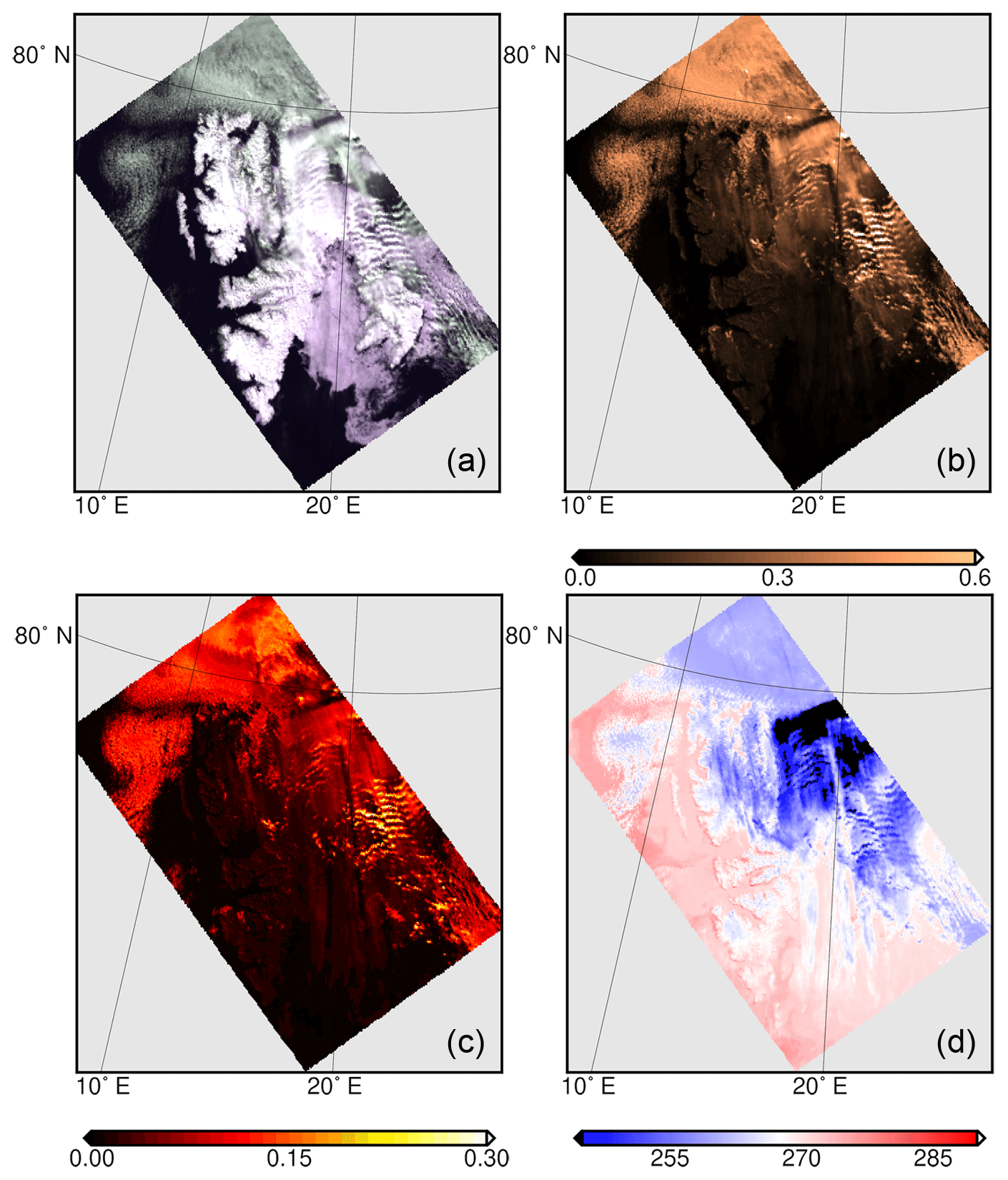
Figure 1(a) The false-colour RGB image of AATSR (using 0.67, 0.87 and 0.55 µm channels) over Svalbard, 10 May 2006, (b) 1.6 µm reflectance, (c) 3.7 µm reflectance, (d) 11 µm brightness temperature.
2.1 AATSR data
The AATSR sensor flown on board polar-orbiting Envisat was primarily designed for measuring sea-surface temperature (SST) with accuracy higher than 0.3 K. As the successor of ATSR-1 and ATSR-2 on European Remote Sensing-1, ERS-1 and ERS-2, AATSR delivered data from March 2002 until Envisat failed in 2012 (http://envisat.esa.int/handbooks/aatsr/CNTR.html, last access: April 2018). The unique design of spectral coverage of AATSR enabled this sensor to measure reflected and emitted radiances in the VIS (0.55, 0.66 µm), NIR (0.87, 1.6 µm) and three TIR channels (3.7, 10.85, 12.00 µm) with spatial resolution of 1×1 km2 at nadir view and swath width of 512 km. In Fig. 1, one example of the AATSR image over Svalbard is shown. It comprises three different wavelengths to highlight the different information, which is retrieved from the wide spectral coverage of this instrument. For example, in the upper-right panel of Fig. 1, the large change in reflectance over snow and ice created a notable contrast between the cloud and the underlying surface at this wavelength compared to that found from the VIS channels used in the R(0.66 µm) G(0.87 µm) B(0.55 µm) image. A similar significant difference between snow/ice and cloud is observed in the reflectance at 3.7 µm, shown in the lower-left panel in Fig. 1. However, at the longer wavelength of 11 µm, thin-cloud patterns appear in the south-western scenes close to and above Svalbard, which have small signatures in the shorter wavelength. Combining the information from the different channels in an appropriate way enables the presence of cloud in the ground scenes to be accurately identified.
The conical imaging geometry of AATSR yields the dual-viewing capability of this sensor. Each scene is imaged twice. The first measurement of the ground scenes is in the forward direction at a viewing angle of 55∘. The second occurs 150 s later at a near-nadir viewing angle. This capability is a design feature of AATSR that delivers an optimal and accurate atmospheric correction and thereby inverts an accurate surface reflectance. The two views theoretically yield independent information about the atmosphere and the surface to be retrieved (http://envisat.esa.int/handbooks/aatsr/CNTR.html). The dual-view approach intrinsically provides more information than the single view for the study of surfaces with complex reflectance characteristics, such as snow and ice (Istomina, 2012). The ASCIA has been applied to AATSR measurements to identify cloud and cloud-free ground scenes.
2.2 SLSTR data
SLSTR on board Sentinel-3A was launched on 16 February in 2016 as the successor to AATSR to provide the continuity of long-term SST measurements. The Sentinel-3B satellite, which contains an identical payload, was also launched by a Rockot/Breeze-KM launch vehicle from the Plesetsk Cosmodrome in northern Russia, on 25 April 2018. The design of the SLSTR instrument has some significant improvements with respect to ATSR (Coppo et al., 2010). For example, the swath widths of single view and dual view were increased from 500 to 1420 and 750 km respectively. This yields global revisit times of 1.9 days at the equator with two satellites and 0.9 day with one satellite. There are measurements of two additional channels in the SWIR, at the wavelengths of 1.37 and 2.25 µm, which are used to provide more accurate cloud, cirrus and aerosol information and used to correct for atmospheric radiative transfer effects in the determination of surface reflectance (Coppo et al., 2010). The Fig. 2 upper right panel shows the use of the new 1.37 µm measurements to detect thin cirrus clouds, which are only weakly identified in reflectance at 3.7 µm, shown in Fig. 2. The current design of ASCIA does not yet include 1.37 µm measurements. This is because the radiance and TOA reflectance at this wavelength are not measured by AATSR. In addition, SLSTR data at this wavelength currently have unresolved calibration issues. Nevertheless, the use of the measurements at this wavelength in thin-cirrus detection should improve the performance of ASCIA in the future. SLSTR also has a higher spatial resolution of 0.5×0.5 km2 in the VIS and SWIR measurements and two channels dedicated to fire detection (Coppo et al., 2010). The use of the observations from SLSTR and AATSR enables a long-term time series of clouds and aerosol parameters to be derived, including AOT over the Arctic. However, there is a ∼4-year gap between the failure of AATSR and the launch of SLSTR. To fill this gap, we will also apply ASCIA to the Advanced Very High Resolution Radiometer (AVHRR) sensor carried by National Oceanic and Atmospheric Administration (NOAA).
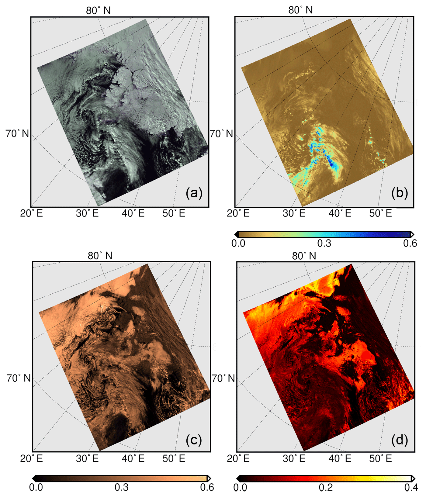
Figure 2(a) The RGB false-colour image (using 0.67, 0.87 and 0.55 µm channels) of SLSTR over Svalbard, 18 April 2017, (b) 1.37 µm reflectance, (c) 1.6 µm reflectance, (d) 3.7 µm reflectance.
2.3 Data used in the cloud identification comparison studies
2.3.1 SYNOP
The SYNOP have been provided by the World Meteorological Organization (WMO) for the purpose of mapping weather information around the world. However, the availability of the data is limited in the Arctic due to the coverage of SYNOP stations in this region. For example, there is almost no observation in the central parts of the Arctic Circle as is shown in Fig. 3. The SYNOP measurements, which are made by an observer or an automated device are available in a standardized layout of numerical code which is called FM-12 by WMO (1995). The SYNOP reports include a variety of meteorological parameters such as temperature, barometric pressure, visibility, etc. as well as cloud amount, which are observed at synoptic hours simultaneously throughout the globe. We used SYNOP cloud fraction, which has a temporal resolution of 1–3 h, to evaluate the performance of our newly developed ASCIA over the Arctic region.

Figure 3SYNOP network coverage over the Arctic, the dark-blue points indicate the location of SYNOP stations.
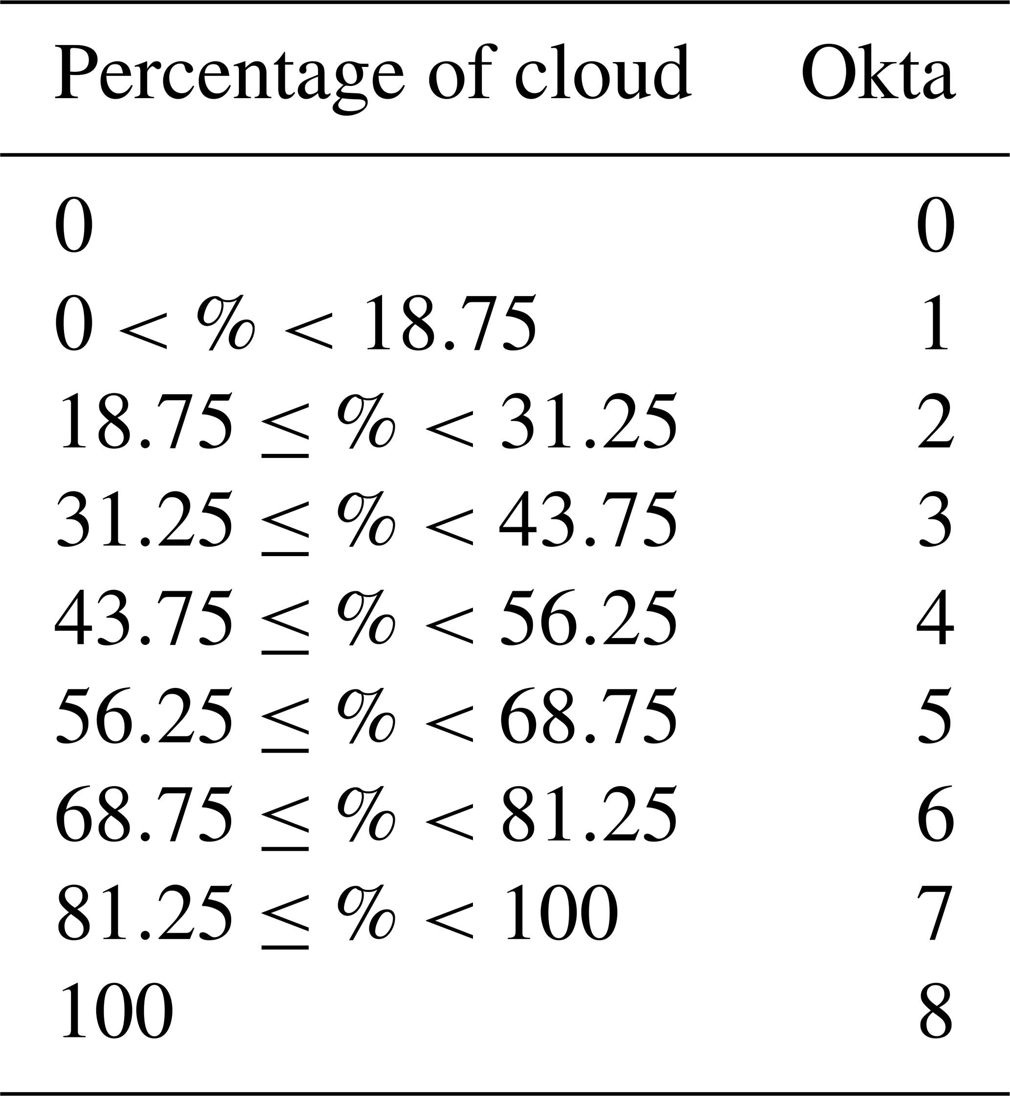
The use of SYNOP measurements to validate a cloud identification algorithm, or for that matter the cloud predicted by a climate model, the fact that the SYNOP cloud fraction is reported using the okta scale, has to be appropriately taken into account. Converting discrete okta values, which range from 0 (completely clear sky) to 8 (completely obscured by clouds), to continuous percentages has been done in different ways by climatologists. A common assumption is that 1 okta equals 12.5 % of cloud coverage (Boers et al., 2010; Kotarba, 2009). For use in this study it was necessary to estimate the error or uncertainty in the okta in measurements. It is assumed that the man-made nature of cloudiness okta estimation has errors of ±1 okta and even larger values of ±2 okta for the non-0 or 8 okta situations (Boers et al., 2010; Werkmeister et al., 2015). Boers et al. (2010) suggested defining a larger range of 18.75 % for 1 okta instead of commonly used value of 12.5 %. We used this approach and defined percentage of cloud values for each okta, which are given in Table 1. More details about the validation procedure are provided in Sect. 5.2.
Table 1Calculation of cloudiness in percentage for corresponding okta values.
2.3.2 AERONET
AERONET is a network of approximately 700 ground-based sun photometers established by National Aeronautics and Space Administration (NASA) and PHOtométrie pour le Traitement Opérationnel de Normalisation Satellitaire (PHOTONS). This globally distributed network aims to provide long-term and continuous measurements of AOT, inversion products and perceptible water in diverse aerosol regimes (Holben et al., 1998). The high temporal resolution of 15 min for these data and expected low accuracy of ∼0.01 to 0.021 (Eck et al., 1999), as well as readily accessible public domain database, provide a suitable data set for aerosol research and characterization.
AERONET data are categorized and available at three levels: level 1.0 (unscreened), level 1.5 (cloud screened and quality controlled) and level 2.0 (quality assured). The data used in this work are selected from level 1.5 to validate cloud identification results from newly developed ASCIA. More details on the validation procedure are discussed in Sect. 5.2.
3.1 Pearson correlation coefficient (PCC)
The PCC was proposed by Pearson (1896) and is used in this study as an indicator of the correlation between sequential AATSR measurements. The PCC is also known as the Pearson product-moment correlation coefficient (PPMCC). It is a standard dimensionless statistical parameter commonly used to measure the strength and direction of the linear association between a pair of variables (Benesty et al., 2009). This parameter has extensively been used in many studies which pursue pattern analysis and recognition.
Our PCC analysis separates the surface reflectance at a given viewing angle, which is stable over short time periods, from the cloud reflectance, which is highly variable over a short time period. To describe the computational procedure developed, we assume x, y to be two random variables. Then the PCC can be written as a function of the covariance of x and y, which is normalized by square root of their variances (Rodgers and Nicewander, 1988; Benesty et al., 2009):
where COV(x,y) is the covariance of variables and σ is the root-mean-square variation of each random variable (Rodgers and Nicewander, 1988; Benesty et al., 2009):
and
where and are the mean values of x and y variables respectively. The correlation coefficient parameter has values between −1 and +1 (Rodgers and Nicewander, 1988). The PCC values were prepared in this study. The association between the two variables is stronger if the absolute value is closer to 1, whereas if two variables are independent or in another word “uncorrelated” PCC value will become 0 (Benesty et al., 2009). As a consequence of the above, the PCC values computed between several data pairs for ground scenes of the same area at different times provide an indication of whether the scene is cloud covered or free of clouds.
For this aim, the use of all seven channels (0.55, 0.66, 0.87, 1.6, 3.7, 11 and 12 µm) was investigated. The visible channels (0.55, 0.66 µm) on their own are not optimal for separating cloud-free scenes from cloudy scenes, in particular for thin clouds. The SWIR and TIR, such as 1.6 µm and beyond, where liquid water and ice absorb provide useful information. There is a large reduction in the reflectance between clear snow/ice and clouds between 0.87 and 1.6 µm (Kokhanovsky, 2006). Our routine takes advantage of this contrast through the PCC calculation. One of the major contributors to error in aerosol retrievals is misclassification of heavy aerosol loads as cloud. Using 1.6 µm reflectance, which is less affected by aerosols than visible wavelengths, in part addresses this issue (Lyapustin et al., 2008).
A second question in PCC analysis (after wavelength selection) is the definition of the optimal size of the block of the ground scene for PCC calculation. In an early version of the current algorithm, we set up 10×10 km2 as the block size. Since aerosol retrieval would be carry out with the same spatial resolution. However, our investigations and previous studies show that 10×10 km2 is not sufficient to capture surface patterns. Thus, blocks of a 25×25 km2 area were used as proposed in previous studies (Lyapustin et al., 2008). The implementation of the PCC analysis as used in this study is discussed in more detail in Sect. 4.
3.2 Reflectance of 3.7 µm thermal infrared channel
The reflectance part of TIR channels at 3.7 and 3.9 µm have been used in different studies to determine cloud properties such as cloud effective radius and thermodynamic phase of the cloud or to discriminate cloud and snow-/ice-covered surfaces (Meirink and van Zadelhoff, 2016; Klüser et al., 2015; Musial et al., 2014; Khlopenkov and Trishchenko, 2007; Pavolonis et al., 2005; Rosenfeld et al., 2004; Spangenberg et al., 2001; Allen et al., 1990). The reason for the wide application of this channel in cloud identification methods is the difference in single-scattering albedo (SSA) at this band compared to shorter VIS and INR wavelengths, which in turn results from the significant sensitivity of SSA to thermodynamic phase and particle size of clouds (Platnick and Fontenla, 2008). For example, the scattering of liquid clouds, having small droplets, is relatively larger than absorption and the ratio of NIR∕VIS reflectance approaches 1. But in the case of large liquid droplets or ice particles, the absorption increases and this ratio is closer to zero (Platnick and Fontenla, 2008). In addition, cloud-free snow reflects at a relatively weak level in comparison to clouds at the 3.7 µm channel (Derrien et al., 1993; Platnick and Fontenla, 2008). Therefore, the contrast due to different physical properties and radiance of snow/ice and cloud at 3.7 µm makes the use of this channel advantageous for the identification of clouds. During the daytime, the measured brightness temperature (BT) at 3.7 µm is determined from the upwelling radiation, which comprises both reflected or scattered solar radiation and the thermal emission from the surface (Musial et al., 2014). To use TOA reflectance at 3.7 µm, procedures are needed to account for and subtract the emission portion of measured BT at 3.7 µm wavelength (Allen et al., 1990). To achieve this goal, independent information about the surface TIR is needed. This is estimated from observations at 11 µm, where absorption by water vapour and other trace gases is small; most objects in regions outside of the tropics can be treated as blackbodies and the measured BT is considered to be in good agreement with real surface temperature (Istomina et al., 2010; Musial et al., 2014).
To do this, we use the method described in Meirink and van Zadelhoff (2016) and Musial et al. (2014), where the reflectance of 3.7 µm can be written as
where R3.7 is the reflectance, i.e. the ratio of scattered radiance to incident solar radiance; L is measured radiance at 3.7 µm, B3.7(T11) is the Planck function radiance (the contribution from thermal emission at 3.7 µm) T11 measurements at 11 µm, F3.7,0 is the solar constant at 3.7 µm and µ0 is the cosine of solar zenith angle.
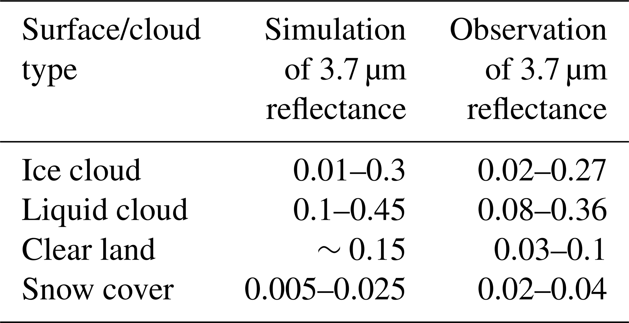
Theoretical reflectance values in the 3.7 µm band, computed by Allen et al. (1990), have been compared to satellite measurements at the same channel from Advanced Very High Resolution Radiometer (AVHRR). The results of this work are summarized in Table 2. According to this study, the reflectance of liquid clouds primarily depends on droplet size and solar zenith angle, whereas for ice clouds, ice particle shape and size distribution are of great importance, along with cloud optical thickness (COT) and sun-satellite geometry. The observed reflectance is reported in a range of 0.08 to 0.36 for liquid clouds and 0.02 to 0.27 for ice clouds (Allen et al., 1990). Arking and Childs (1985) calculated 3.7 µm reflectance for ice clouds, which varies between 0.01 to 0.30 for the COT of 0.1 to 100 and ice crystal effective radius of 2 to 32 µm, solar zenith angle of 60∘. Spangenberg et al. (2001) reported a typical value of 0.04 to 0.4 for clouds. In the case of a snow-covered surface, 3.7 µm reflectance is dependent on many factors including snow grain size, solar zenith angle, liquid water content, snow impurities, etc. Considering the snow grain size of 50 to 200 µm, with a solar zenith angle of 40 to 80∘, the modelled values for snow reflectance varies between 0.005 and 0.025 at 3.7 µm (Allen et al., 1990). However, a range of 0.02 to 0.04 is observed from the satellite measurements over the same wavelength for snow cover. This difference between model calculations and measurements is explained by snow impurities (Allen et al., 1990). For land areas, the 3.7 µm reflectance is impacted by soil type, vegetation type, coverage and moisture content. An average value of 0.15 is derived for clear sky land scenes at 3.7 µm (Allen et al., 1990). In order to use the remarkable contrast between snow cover and clouds in the 3.7 µm channel, two main issues have to be taken into account: (1) the interference between snow and ice-cloud values; (2) the interference between cloud and land reflectance. The latter is easily solved by using information from visible channels with 3.7 µm reflectance. This is because land scenes in polar region are dark in comparison to cloud and snow. The first issue, discriminating ice clouds from snow, is a challenging task. To detect ice clouds, we combined 3.7 µm reflectance with PCC analysis. A full description of this new method is given in Sect. 4.
Table 2Simulated and observed reflectance values at 3.7 µm (Allen et al., 1990).
The ASCIA implementation is initiated by preparing a time series of data. A time span of 1 month for the ground scene was selected. Hagolle et al. (2015) indicated that in Sentinel-2 measurements with revisit time of 5 days, most of the given scenes would be observed cloud-free at least once a month. Consequently, we also assume that every scene of AATSR measurements, which have a higher revisit time of 3 days, will be cloud-free at least once a month.
Depending on the latitude and the time of year, the number of downloaded data varies from 10 to 50 or more over the same scene. AATSR provides more data over higher latitudes, which increase in spring and summer due to longer polar days and solar illumination. The AATSR L1b data are already provided as gridded and calibrated 1×1 km2 scenes. These include geolocation information interpolated from the tie-point scenes, which are equally distributed across a single AATSR image (http://envisat.esa.int/handbooks/aatsr/CNTR.html). Consequently, there is no necessity to regrid them for the georeferencing step. This is considered an advantage, because it preserves the original reflectance value of each scene for the following steps. However, the time series data are acquired by the satellite from different viewing geometries. To compute PCC values over the same areas from different days, ASCIA selects the closest similar scenes using geolocation information provided in the data. The closest distance is often found to be within 0.006∘ and increases to 0.01∘ in the worst case and thus is considered to be of negligible significance. After using this procedure to select the observations, ASCIA comprises two main parts that identify the presence of cloud: (i) a PCC analysis at 1.6 µm and (ii) the use of thresholds for reflectance of 3.7 µm channel.
In the first step, a PCC analysis for a block of ground scenes (25×25 km2) is used to identify cloud and cloud-free blocks, which are assumed to have low and high PCC values respectively. The output of this step is a binary flag at the block level. This serves as input for the second step to produce a binary ground flag at ground scene level (1×1 or 0.5×0.5 km2 depending on spatial resolution of instrument) cloud identification, by using the knowledge of the reflectance of solar radiation in the 3.7 µm channel. The combination of these two constraints is necessary because neither PCC analysis nor reflectance part of 3.7 µm channel are adequate on their own for accurate cloud detection. A high PCC value cannot guarantee the clearness of the whole block of scenes (Lyapustin et al., 2008) because some ground scenes may still contain clouds, which are not enough in number to significantly decrease the PCC value. This case occurs frequently over small or semi-transparent clouds, where the textural pattern of surface is still observable through the clouds (Lyapustin et al., 2008). Small PCC values may be caused by rapid surface change, high aerosol load or a lack of recognizable spatial patterns, which is often the case over homogeneous snow-covered surfaces (Lyapustin et al., 2008). A PCC value of 0.63 is suggested by Lyapustin et al. (2008) to separate cloud-free blocks over midlatitudes. Considering fewer surface patterns in a large area of the Arctic compared to lower latitudes, and our PCC analysis over both middle and high latitudes, we defined a lower threshold for PCC of 0.4 over the Arctic region and found that a PCC of 0.6 is appropriate for midlatitudes based on a number of statistical analyses.
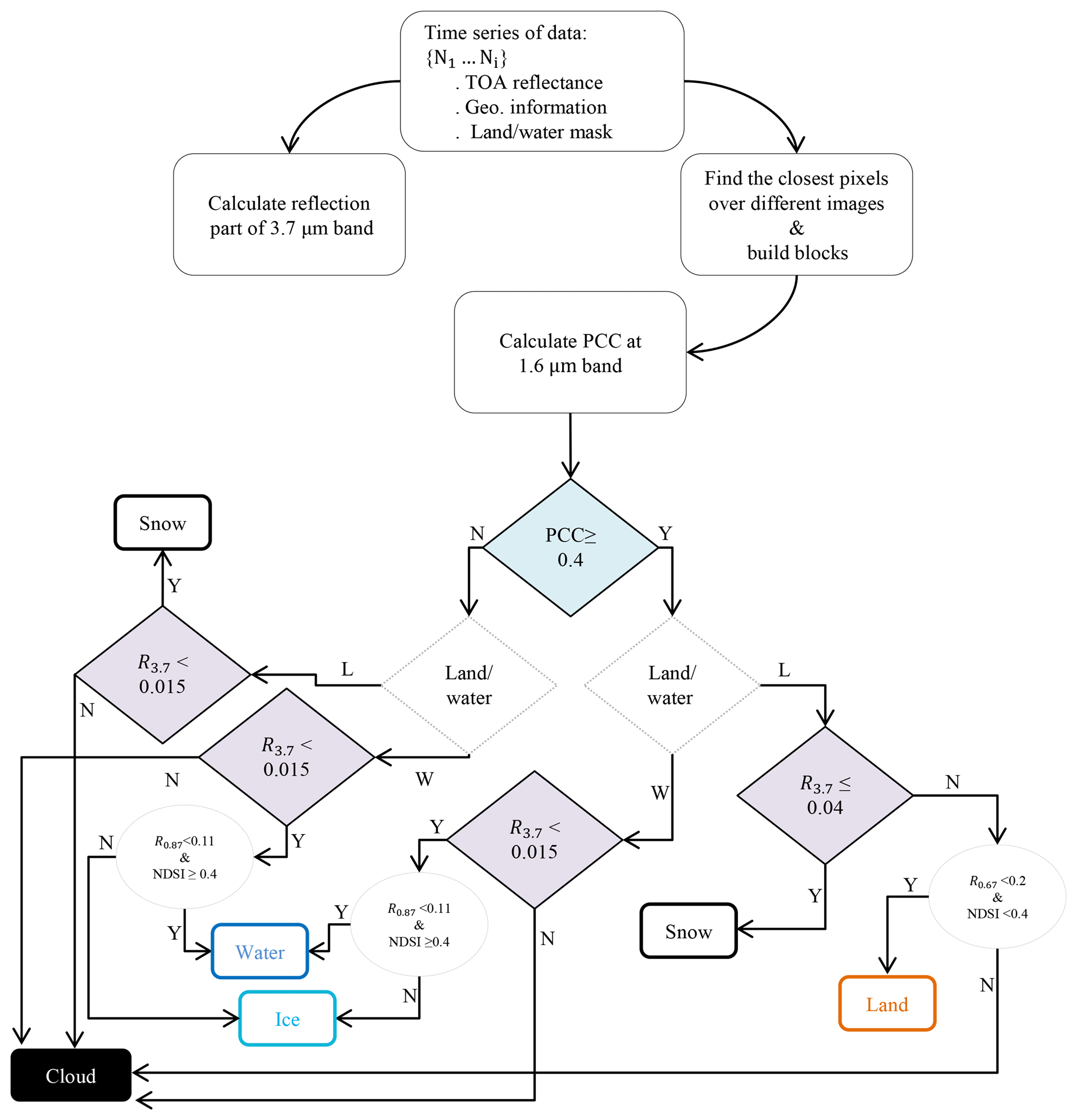
After computing the first binary cloud flag at block level using the last measurement and one previous image, ASCIA keeps the result in memory and repeats the procedure with the second-to-last data. This procedure is iterated until the last measurement of the data series is involved. The final binary blocks are imported in the second step to identify cloudy scenes based on thresholds defined differently for blocks with low and high PCC value. We note that, the snow/ice reflectance in the 3.7 µm channel (∼0.005–0.025) has interference with those of ice clouds (0.01–0.3) at this wavelength. To avoid the uncertainty arising from this problem, we defined the PCC analysis as a decision point of ASCIA requiring further optimized analysis:
- i.
For the high PCC ≥0.4, the whole block is considered to be cloud-free and then ASCIA starts looking for remaining small cloud scenes within a block, i.e. scenes with R3.7 larger than the maximum value observed over snow at 3.7 µm: R3.7>0.04 (Allen et al., 1990).
- ii.
For PCC <0.4, the block is assumed to be cloudy; ASCIA removes all scenes within the block and only keeps scenes which satisfy the R3.7<0.015 test. This threshold is equal to or lower than the lowest observation of ice cloud reflectance at 3.7 µm (Allen et al., 1990).
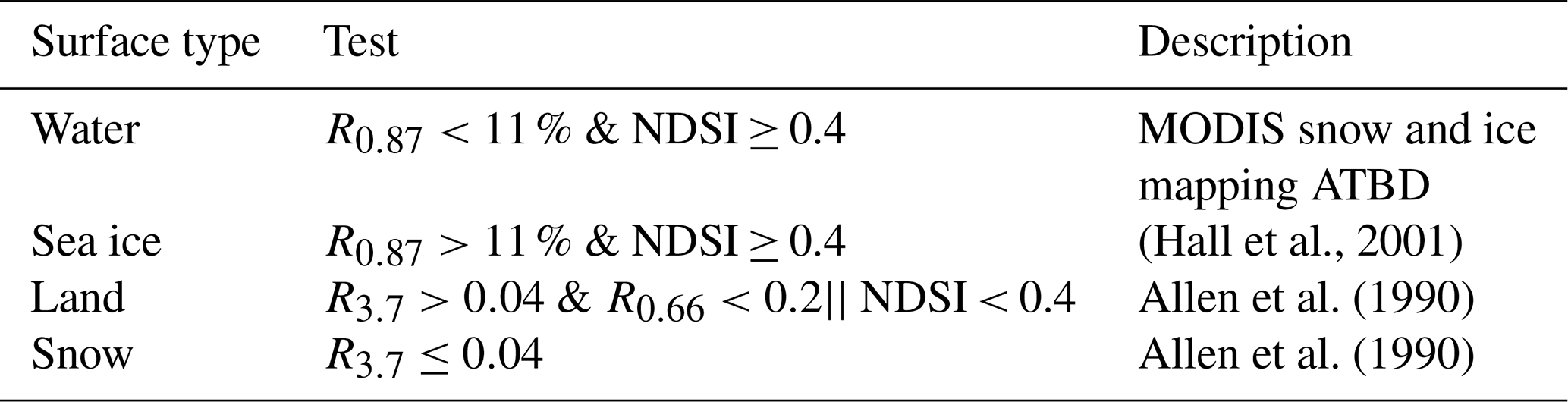
In our method, the PCC analysis constrains the procedure and the strict decision is only made within low PCC blocks. The loss of some clear scenes in low PCC blocks is an unavoidable side effect of using these strict criteria, in particular over land scenes, which have low PCC and high 3.7 µm reflectance values. However, ASCIA detects the presence of thin-cirrus cases with a relatively high confidence level. A schematic flow chart of ASCIA is shown in Fig. 4, with the use of the two main constraints being highlighted. In addition to picking out clear scenes, a simple land classification procedure is undertaken in this step of ASCIA. Snow/ice scenes are identified with low 3.7 µm reflection, whereas land scenes with high reflection are classified with the aid of the darkness test over visible channels. The corresponding thresholds for land classification scheme are described in the Table 3.
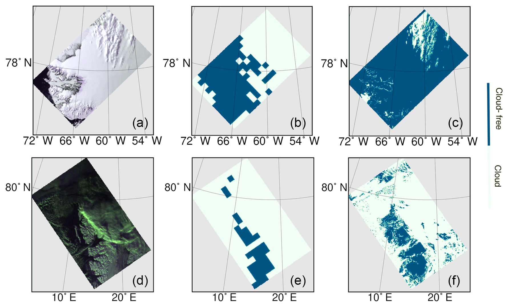
Figure 5Examples of the results of ASCIA on AATSR observations on the scenes over Greenland (a–c) between 75∘ N, 48∘ W; 75∘ N, 75∘ W; 81∘ N, 48∘ W and 81∘ N, 75∘ W, taken on 18 May 2008 and Svalbard (d–f), within 75∘ N, 4∘ E; 75∘ N, 32∘ E; 81∘ N, 4∘ E and 81∘ N, 32∘ E on 1 March 2008. (a, d) RGB false-colour images (using 0.67, 0.87 and 0.55 µm channels), (b, e) cloud detection at block level (25×25 km2), (c, f) cloud detection at scene level (1×1 km2).
Although characterized as land, a scene may include soil, different types of vegetation cover or even melting snow. The latter mixes with soil and becomes dark enough to be filtered out from the snow class. Sea ice is distinguished from water on the basis of its greater brightness; one scene might be white enough to be considered as ice. However, melting or broken ice, as well as new ice, would not be labelled as ice. Snow over sea ice is not distinguished from pure sea ice and both of them are labelled as sea ice. This also means that ice over land is also marked as snow as well as pure snow.
A representative example of the block level (25×25 km2) and scene level (1×1 km2) results of ASCIA applied to AATSR observations is shown in Fig. 5. This example was selected to show the performance of ASCIA in the presence of different surface conditions: (1) one scene is over a combination of fairly homogeneous snow cover, land, ocean, sea ice and cloud scene in the north-west of Greenland, taken on 18 May 2008; (2) another example is over a surface with highly variable topography over Svalbard with relatively higher solar zenith angle (>80∘) on 1 March 2008. As we discussed earlier, the ambiguity of the PCC analysis over homogeneous surfaces on the right and left sides of the AATSR scene in the middle panel of Fig. 5 is compensated in the right panel by using additional information from the 3.7 µm channel.
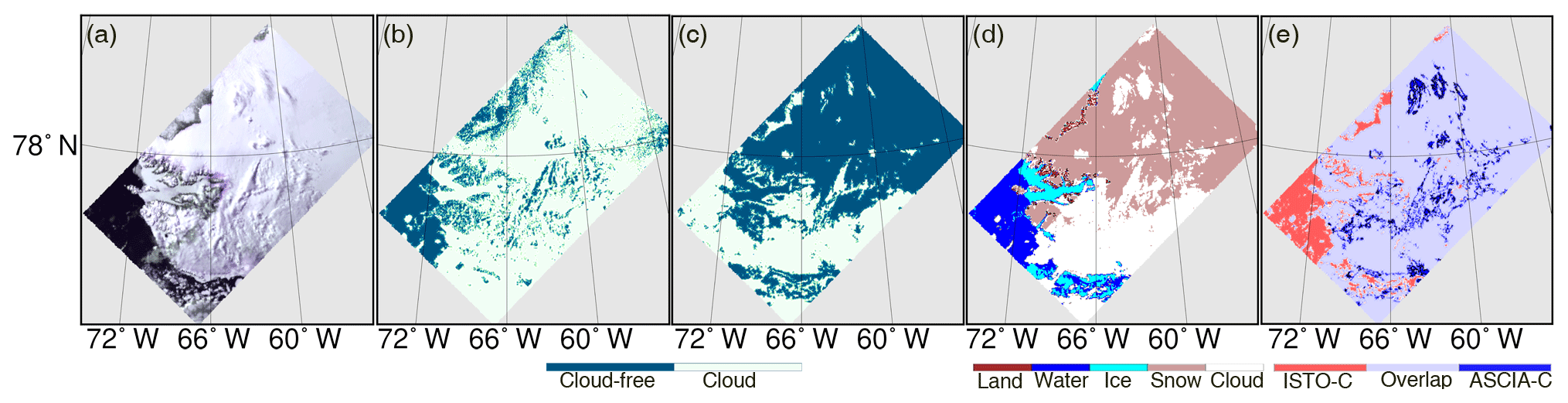
Figure 6(a) The RGB false-colour image (using 0.67, 0.87 and 0.55 µm channels) of AATSR over northern Greenland, 24 May 2008; (b) nadir cloud flag from the AATSR L2 product; (c) cloud detection based on the spectral shape of clear snow; (d) cloud detection of ASCIA and (e) the difference between ISTO and ASCIA.
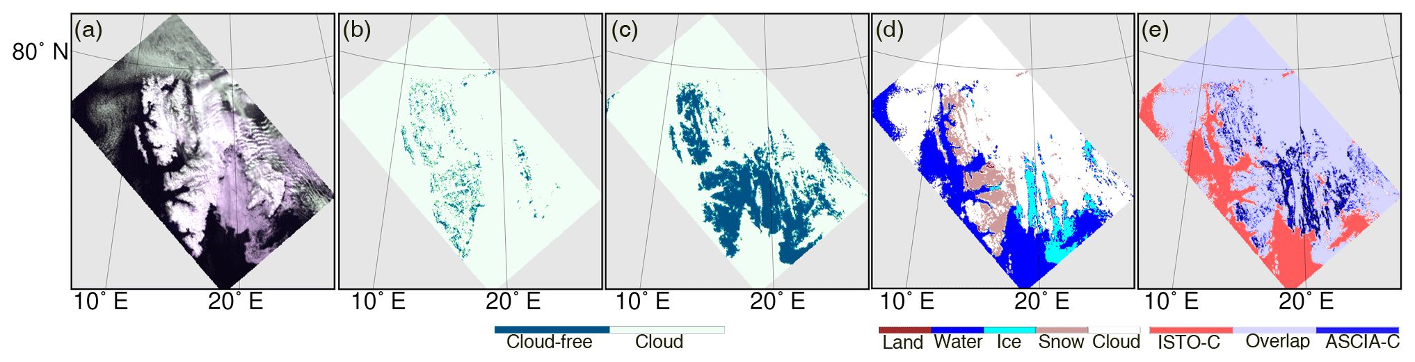
Figure 7(a) The RGB false-colour image (using 0.67, 0.87 and 0.55 µm channels) of AATSR over Svalbard, 10 May 2006; (b) nadir cloud flag from the AATSR L2 product, (c) cloud detection based on the spectral shape of clear snow, (d) cloud detection of ASCIA and (e) the difference between ISTO and ASCIA.
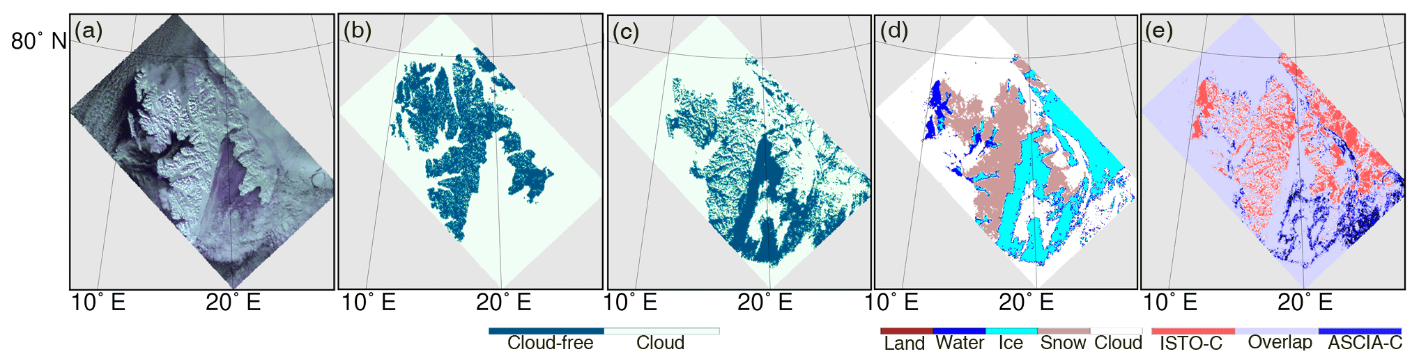
Figure 8(a) The RGB false-colour image (using 0.67, 0.87 and 0.55 µm channels) of AATSR over Svalbard, 18 March 2008; (b) nadir cloud flag from the AATSR L2 product; (c) cloud detection based on the spectral shape of clear snow; (d) cloud detection of ASCIA and (e) the difference between ISTO and ASCIA.
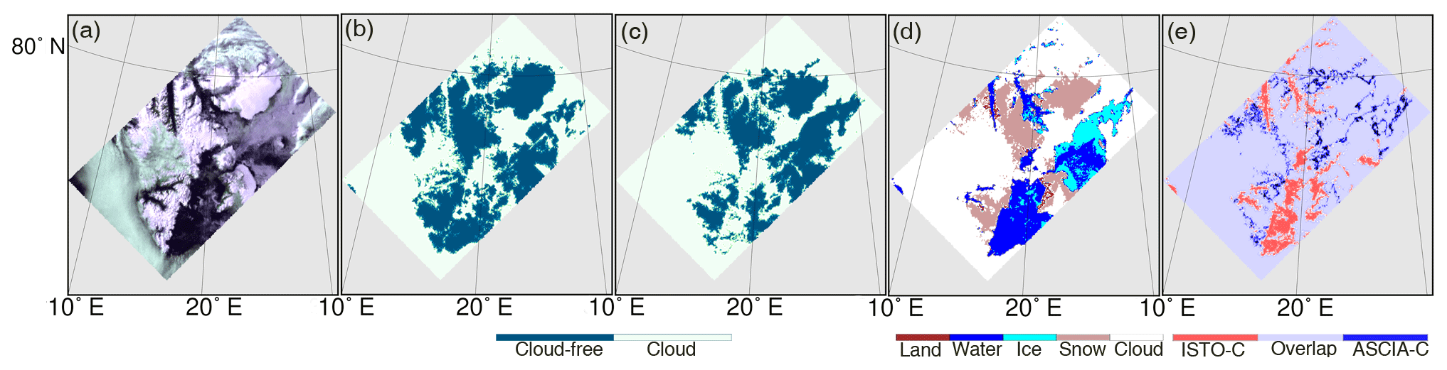
Figure 9(a) The RGB false-colour image (using 0.67, 0.87 and 0.55 µm channels) of AATSR over Svalbard, 6 July 2008; (b) nadir cloud flag from the AATSR L2 product; (c) cloud detection based on the spectral shape of clear snow; (d) cloud detection of ASCIA and (e) the difference between ISTO and ASCIA.
5.1 The comparison of ASCIA products with products from other algorithms using space-borne observation
In this study, we applied our recently developed ASCIA to identify cloud in the scenes using AATSR L1b (TOA reflectance) and SLSTR L1b gridded data. The input file to the process chain is one scene of the AATSR L1b product. The output comprises five classes of surface types, including snow/ice, sea ice, water, cloud and land. The procedure of surface classification is explained in Sect. 4. The location and time of selected case studies are used to show that the identification of cloud by our new ASCIA is adequate. The AATSR data are selected from several years starting from 2006, during strong Arctic haze episode, which originated predominantly from agricultural fires burning in eastern Europe. The event has been reported previously (Law and Stohl, 2007). A second episode in 2008 is also considered, for which validation data are available from SYNOP stations. Three months of data from March, May and July have been acquired over Greenland and Svalbard to assess the performance of ASCIA in a wide range of solar zenith angles (60–85∘), surface and atmospheric conditions observed at high latitudes. In order to take various surface types in the Arctic into account, we selected case studies including highly variable topography and fairly homogeneous snow cover, coast lines, land and ocean along snow and ice-covered surface. The designed criteria for ASCIA are optimized for various regions over the Arctic observed under different solar illumination conditions. Polar night and transition seasons in low light conditions are excluded from our retrievals. The results obtained are compared with (i) the AATSR L2 nadir cloud flag; (ii) those results obtained with ISTO (Istomina et al., 2010) and (iii) MODIS.
As we discussed in Sect. 1, misclassification of thin cirrus cloud with clear snow is reported to be an unresolved problem of ISTO approach. Two representative scenarios of this problem are illustrated in Figs. 6 and 7 over Greenland and Svalbard respectively, in which thin cloud is detected as clear snow by the ISTO method, whereas ASCIA confirmed the presence of cloud. Over a homogeneous surface such as Greenland, the second step of ASCIA is decisive. The lack of structural patterns on the surface leads to low PCC values in the first step and consequently an overestimation of cloudy scenes. However, the reflection part of 3.7 µm could help to label and bring back clear homogeneous surface as cloud-free snow in second step. The right panel in Figs. 6 and 7 shows the difference between the result of ASCIA and ISTO. In this panel, the dark-blue scenes show clouds, which are not detected by ISTO but are by ASCIA. The reddish scenes show cloud-free cases, which ISTO fails to detect, but are correctly labelled by ASCIA as cloud-free. In addition to the edge of clouds, which are difficult to detect over snow and ice, there are a significant number of undetected cloud scenes in ISTO results, which are identified successfully by ASCIA. However, for the rest of these two scenes, the two algorithms show good agreement.
The ESA cloud product from L2 data overestimates cloud, which leads to a loss of clear snow and ice scenes. The tendency of this product to flag clear scenes as cloud is also visible in Figs. 6 and 7. The results in Fig. 8 show undetected clouds as another problem of the AATSR level 2 cloud product, which happens frequently at high solar zenith angles. To have a better understanding of this misclassification, we validated the AATSR L2 nadir cloud flag against SYNOP measurements and the results are described in Sect. 5.2.
Poor performances for cases over the Arctic with high solar zenith are observed in all of the results using ISTO method. Figure 8 is an example for Svalbard in March 2008. Over a highly variable surface type, such as Svalbard, the reflection at 3.7 µm can approach high values such as 0.035, which is similar to that from cloud reflection. In this case, PCC analysis is of great importance for keeping cloud-free snow scenes from the strict criteria of the second step, in particular in cases with higher solar zenith angles. ASCIA in a high PCC block covers a wide range of solar zenith angles (40–80∘) and results in the reflectance of snow/ice being defined between 0.02 and 0.04 in the 3.7 µm channel. In the right panel of Fig. 8, a relatively large number of red scenes are observed, which are falsely detected as cloud by the ISTO method.
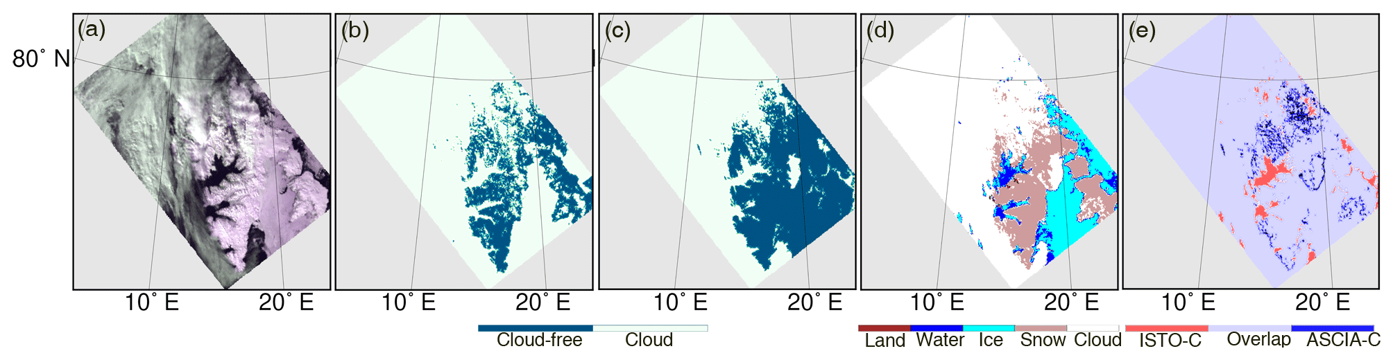
Figure 10(a) The RGB false-colour image (using 0.67, 0.87 and 0.55 µm channels) of AATSR over Svalbard, 3 May 2006; (b) nadir cloud flag from the AATSR L2 product; (c) cloud detection based on the spectral shape of clear snow; (d) cloud detection of ASCIA and (e) the difference between ISTO and ASCIA.
Figure 10 shows one example of a haze event over Svalbard on 3 May 2006. Both the ESA and ISTO cloud products showed good results for this case with the exception of thin-cloud scenes, which are falsely labelled as clear snow by ISTO. The appropriate design and application of PCC analysis over 1.6 µm enables cloud to be discriminated from a heavy aerosol load. However, aerosol loads over cloud could not be separated from cloudy scenes.
The only season in which all three approaches detected clouds with similar success was in July, as shown in Fig. 9. Although ASCIA shows an overall better performance, in particular for thin clouds, the required computational time for cloud detection and surface classification is higher than for the two other methods.
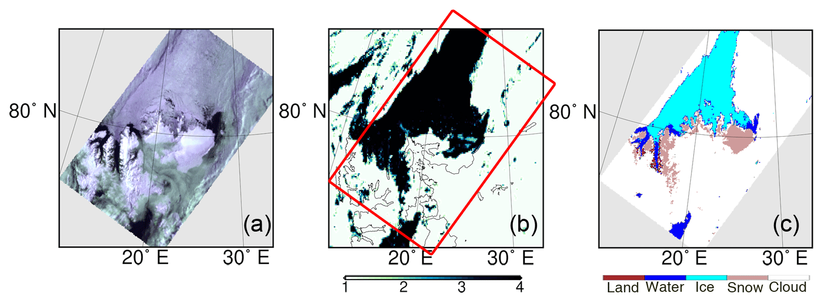
Figure 11(a) RGB false-colour image (using 0.67, 0.87 and 0.55 µm channels) of AATSR over Svalbard, 14 July 2008, 16 h 40 min 45 s, (b) MODIS cloud mask algorithm retrieved data: 1 is cloudy, 2 is probably cloudy, 3 is probably clear, 4 is clear (red rectangle shows the coverage of AATSR) for 16 h 25 min, (c) the results for the cloud detection of ASCIA.

Figure 12(a) RGB false-colour image (using 0.67, 0.87 and 0.55 µm channels) of AATSR over Greenland, 18 May 2008, 23 h 13 min 38 s, (b) MODIS cloud mask: 1 is cloudy, 2 is probably cloudy, 3 is probably clear, 4 is clear (red rectangle shows the coverage of AATSR) for 23 h 5 min, (c) cloud detection of ASCIA.
We also compared our results with those from the MODIS cloud identification algorithm, used for masking cloudy scenes. As an example, Fig. 11 shows the AATSR scene over Svalbard on 14 July 2008, where a large part of the sea ice is covered with thin clouds, which have a small signature in the visible channels. The middle panel shows the MODIS cloud mask for the same area. Although there is a small time difference of 15 min between MODIS and AATSR overpasses, we see that scenes identified as cloudy by ASCIA correspond well with those of MODIS.
Figure 12 shows another example over the north-west of Greenland on 18 May 2008. The thin and broken clouds are well detected over the snow cover by ASCIA, as well as the clouds over the southern part of the scene, which is covered with snow and ocean. As we can see from the comparison between ASCIA and MODIS cloud scene identification, cloudy scenes in the northern part of scene are not captured by the MODIS product, but the presence of clouds is seen in the RGB image in the left panel. We observed other cases with similar differences, especially for thin and broken clouds. There are two potential sources of these differences: (1) time differences, which are 10 min in this case, or (2) an inadequate performance of the MODIS cloud mask over bright surfaces covered by snow and ice.
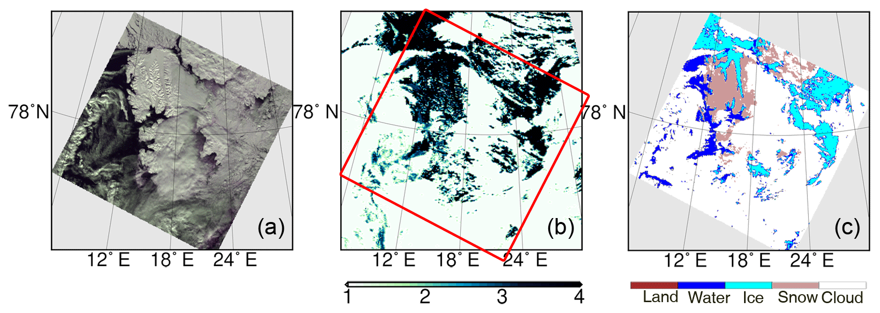
Figure 13(a) The RGB false-colour image (using 0.67, 0.87 and 0.55 µm channels) of SLSTR over Svalbard, 18 April 2017, 10 h 15 min 6 s, (b) MODIS cloud mask: 1 is cloudy, 2 is probably cloudy, 3 is probably clear, 4 is clear (red rectangle shows the coverage of AATSR) for 11 h 30 min, (c) cloud detection of ASCIA.
Due to the loss of Envisat and thus AATSR data in 2012 and the need for long time series of consistent data, we tested ASCIA on the AATSR successor SLSTR as well. Figure 13 shows some results over Svalbard on 18 April 2017. Due to the smaller swath width of AATSR compared to SLSTR, ASCIA is not applied to the full coverage of SLSTR and the selected scene is cropped to have a similar coverage of 500×500 km2. In spite of some unresolved calibration issues in this sensor, the higher spatial resolution in SLSTR clearly helps to improve cloud identification in the first step, because the PCC analysis is more sensitive to smaller changes in 0.5×0.5 km2 scenes compared to 1×1 km2. Moreover, the shorter revisit time of the Sentinel-3 satellite provides more acquired images over the same scene. This results in a larger number of reference images compared to those from Envisat. Overall these effects result in an expected improved performance of ASCIA when applied to SLSTR data compared to when it is applied to AATSR. The comparison of MODIS and ASCIA results indicates that ASCIA detected more cloudy scenes than the MODIS algorithm in agreement with the above.
5.2 The comparison to ground-based measurements: SYNOP and AERONET
In this section, we present a quantitative validation of our ASCIA results by making comparisons with simultaneous ground-based SYNOP and AERONET measurements. The ESA standard cloud product is also compared with these validation data sets. The difference in spatial and temporal resolutions of the new cloud identification data sets and the data sets used to validate this data set have to be taken into account. To define the optimal maximum temporal difference between SYNOP and satellite data, other comparable validation activities used different temporal intervals like 10 min (Werkmeister et al., 2015), 15 min (Musial et al., 2014), 1 h (Dybbroe et al., 2005) and 4 h (Meerkötter et al., 2004). The investigation and results in the previous publications indicate that temporal differences in validation of satellite retrievals against SYNOP depend on meteorological conditions. Allowing only a small temporal difference between measurement data sets (here, SYNOP and ASCIA) ensures an optimal temporal overall but can introduce a significant sampling error due to the small number of scenes for validation (Bojanowski et al., 2014). According to Bojanowski et al. (2014) a temporal difference of 90 min between measurement data sets (SYNOP measurements at a temporal resolution of 3 h and satellite retrievals) minimizes the sampling error. However, a potentially longer temporal difference will introduce an error which should be considered along other sources of uncertainty (different viewing perspective, different spatial footprint, etc.). In this study, the maximum allowed temporal difference between the ASCIA retrievals and SYNOP measurements is less than ±20 min in most cases and generally does not exceed ±45 min. To compare surface measurements from the SYNOP hemispheric view with the cloud identification at a spatial resolution of 1×1 km2, we calculated cloudiness as the percentage of cloudy scenes within a window of 20×20 km2 around each SYNOP station. This is a similar distance to that used in previous studies to validate satellite-based cloud identification SYNOP or similar surface measurements (Kotarba, 2017; Werkmeister et al., 2015; Minnis et al., 2003). The cloud detection data product was then compared to the 3 selected months (March, May and July) of SYNOP observations. These result in 100 measurements over Svalbard and Greenland.

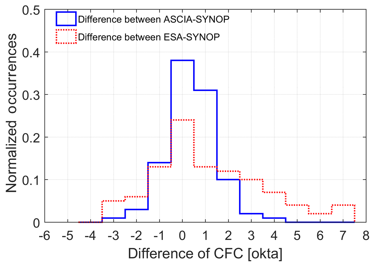
Figure 15Histogram of CFC differences (blue is ASCIA minus SYNOP; red is ESA cloud product minus SYNOP).
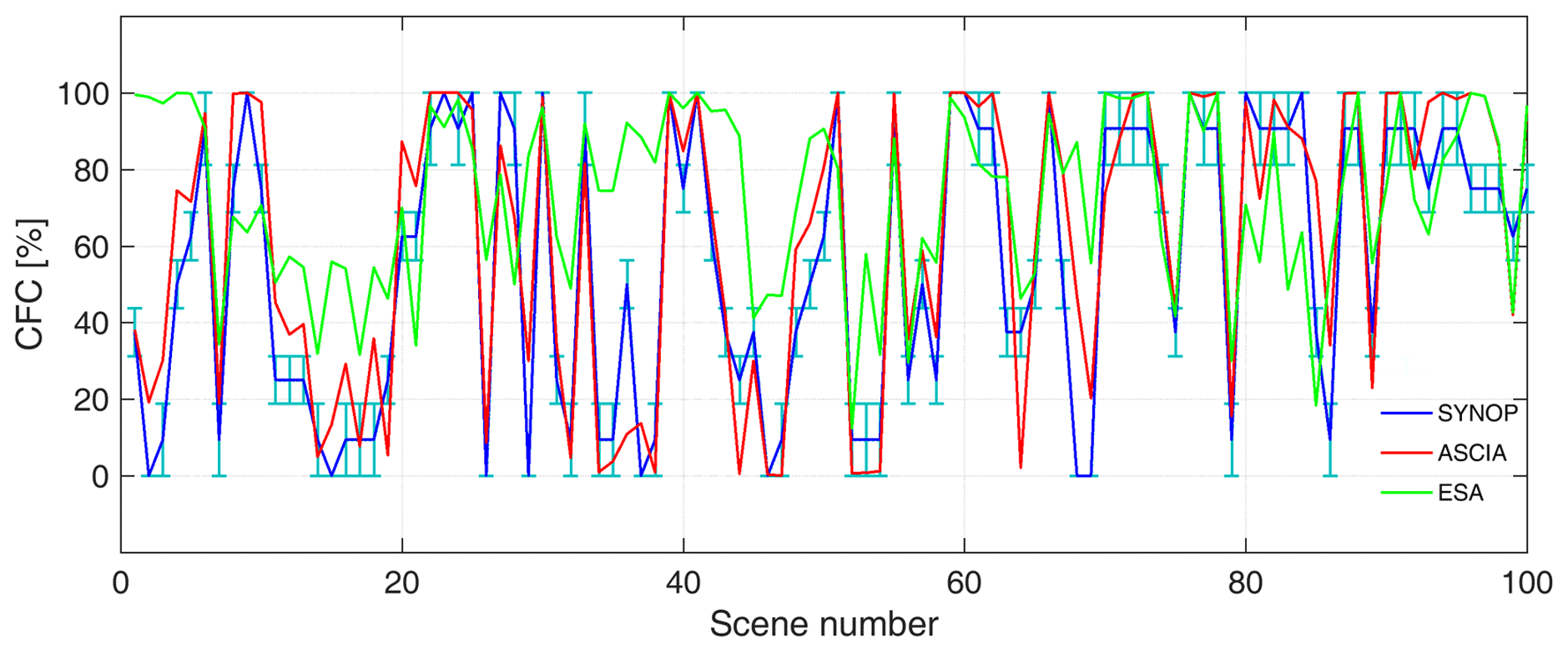
Figure 16CFC in percent by ASCIA (red), SYNOP (blue) and ESA Cloud Product (green) for 100 scenarios in March, May and July 2008 over Svalbard and Greenland. Light-blue error bars show the range of percentage values for each okta from SYNOP measurements.
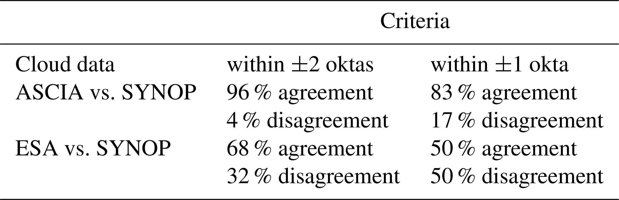
In Fig. 14 we present the relation between the calculated cloud fractional cover (CFC) from ASCIA and SYNOP measurements and density plot of occurrences of the CFC by ASCIA as a function of SYNOP, following the idea of Werkmeister et al. (2015). The two data sets have a correlation coefficient of R=0.92. In 31 % of scenarios, ASCIA estimates 1 okta more than SYNOP, while in 14 % of match-ups SYNOP shows a higher CFC of 1 okta. Figure 14 also reveals that most of the ±1 okta differences occur when either SYNOP or ASCIA estimate 7 or 8 oktas, which could be due to the definition of 8 oktas (100 % CFC) and conversion of a continuous percentage to okta (Werkmeister et al., 2015). For instance, CFC of 99.9 % is considered as 7 oktas by using Table 1, but the CFC difference is only 0.1 % with 8 oktas. The underestimation of CFC by SYNOP is also indicated in the histogram of the difference between ASCIA and SYNOP in Fig. 15. This underestimation was confirmed by previous studies as well (Kotarba, 2009; Werkmeister et al., 2015). We also indicate the higher accuracy of ASCIA for cloud detection compared to the ESA cloud product. The results of the validation are summarized in Table 4. The cloud cover reported from SYNOP agrees in 96 % (within ±2 okta) and 83 % (within ±1 okta) of the observations with the cloud identification data from ASCIA. As discussed earlier, an error of ±1 to ±2 okta would be expected as the accepted accuracy range from SYNOP cloud cover values due to the man-made nature of its observation and viewing conditions (Boers et al., 2010; Werkmeister et al., 2015). In comparison, the ESA cloud product agrees 68 % (within ±2 okta) and 50 % (within ±1 okta) with SYNOP CFCs. The larger differences between the SYNOP and ESA cloud products are also indicated in Fig. 16, where the CFC values are shown as percentages for ASCIA, ESA and SYNOP for the validation scenarios. The blue error bars indicate the range of okta values for each SYNOP as explained in Table 1.
Table 4A summary of the comparison of ASCIA and ESA cloud products with SYNOP measurements used to validate these products.
We also validated ASCIA cloud identification results with AERONET level 1.5 measurements, which are cloud screened. The procedure for this validation takes place in two steps: (1) covering AERONET-observed AOT to a cloud flag (AOT is provided in AERONET only in cloud-free conditions) and(2) validation of ASCIA with AERONET cloud flag. In 86.1 % of 36 studied scenes over Svalbard, both ASCIA and AERONET confirm the presence of clouds.
A new cloud detection algorithm, called ASCIA, has been developed for use at high altitudes above bright surfaces to generate stand-alone products and for subsequent use in the retrieval of AOT over the Arctic. ASCIA has been developed for use with the data from the European instrument AATSR on the ESA Envisat (2002 to 2012) and SLSTR on ESA Sentinel-3A or -3B. ASCIA initially employs a time series analysis of PCC to identify cloud presence, the stability and cloud-free conditions on the block scale of scenes (25×25 km2). It then uses the 3.7 µm solar reflectance to discriminate cloud presence at the spatial resolution of the scene, which is 1×1 or 0.5×0.5 km2 for AATSR and SLSTR measurements respectively. The PCC parameter analysis of a block of data is independent to a first approximation of threshold settings, which often leads to misclassification of cloud and snow due to the similarity of their spectral characteristics and thus the thresholds. The brightness temperature measurements from the 3.7 µm channel provide information used to convert a block-level resolution (25×25 km2) to a scene-level resolution (1×1 or 0.5×0.5 km2) cloud identification. ASCIA thereby exploits the contrast in reflectance between snow/ice and cloud at 3.7 µm wavelength.
The results of applying the newly developed ASCIA are compared and validated against five existing products and methods over the Arctic: (1) SYNOP measurements, (2) AERONET measurements, (3) one of the existing methods based on the spectral shape of clear snow, (4) AATSR L2 nadir cloud flag, (5) MODIS cloud product. The validation resulted in an overall agreement of 96 % (within ±2 oktas) and 83 % (within ±1 okta) between SYNOP and ASCIA. The comparison of the ASCIA and ISTO methods shows the improved performance of ASCIA in extreme situations, such as high solar zenith angle conditions.
The validation results indicate that the current ESA AATSR L2 nadir cloud flag often falsely identifies clouds over snow/ice, except during summer. The comparison between the ESA AATSR L2 cloud product and SYNOP measurements resulted in an agreement of 68 % (within ±2 oktas) and 50 % (within ±1 okta). The overall better performance of ASCIA has also been demonstrated when it is applied to the SLSTR data. Nevertheless, optimization is needed for the detection of cloud over land (soil, vegetation, etc.) for the PCC blocks with lower values. This is because the strict performance of ASCIA in cloudy blocks results in scenes of clear land (without snow cover) being identified as cloud due to high reflectance of land scenes in the 3.7 µm channel. We also note that sub-scene cloud detection has not been studied with the current version of ASCIA. The use of reflectance in the 1.37 µm channel will be tested in the future to improve thin-cirrus detection in ASCIA. The objective of this study was to assess and validate the current version of ASCIA for daytime observations. An adaption of ASCIA is planned to identify clouds at night.
The AATSR, SLSTR, MODIS and AERONET data are publicly available: AATSR: http://ats-merci-ds.eo.esa.int/merci/queryProducts.do (last access: June 2018); SLSTR: https://coda.eumetsat.int (last access: June 2018); MODIS: https://modis-atmos.gsfc.nasa.gov (last access: June 2018); AERONET: https://aeronet.gsfc.nasa.gov (last access: June 2018); Due to the strict data policy of DWD, the SYNOP data are not publicly accessible and we received these data from Rainer Hollmann (rainer.hollmann@dwd.de). The ASCIA data can be accessed upon request to the corresponding author (jafari@iup.physik.uni-bremen.de).
SJ designed and developed the algorithm, performed the analyses, validated the results and prepared the manuscript. LM, MV and JPB supervised the research project and contributed to the writing and revision of the manuscript. VR provided general advice and valuable discussions on the paper and the work. RH provided the SYNOP data.
The authors declare that they have no conflict of interest.
This article is part of the special issue “Arctic mixed-phase clouds as studied during the ACLOUD/PASCAL campaigns in the framework of (AC)3 (ACP/AMT inter-journal SI)”. It is not associated with a conference.
We gratefully acknowledge the funding by the Deutsche Forschungsgemeinschaft
(DFG, German Research Foundation) – project number 268020496 – TRR 172,
within the Transregional Collaborative Research Center “ArctiC
Amplification: Climate Relevant Atmospheric and SurfaCe Processes, and
Feedback Mechanisms (AC)3”.
The article
processing charges for this open-access publication were covered by the
University of Bremen.
Edited by: Jost
Heintzenberg
Reviewed by: two anonymous referees
Allen, R. C., Durkee, P. A., and Wash, C. H.: Snow/cloud discrimination with multispectral satellite measurements, J. Appl. Meteor., 29, 994–1004, https://doi.org/10.1175/1520-0450(1990)029<0994:SDWMSM>2.0.CO;2, 1990.
Arking, A. and Childs, J. D.: Retrieval of cloud cover parameters from multispectral satellites images, J. Clim. Appl. Meteorol., 24, 322–333, https://doi.org/10.1175/1520-0450(1985)024<0322:ROCCPF>2.0.CO;2, 1985.
Arola, A., Eck, T. F., Kokkola, H., Pitkänen, M. R. A., and Romakkaniemi, S.: Assessment of cloud-related fine-mode AOD enhancements based on AERONET SDA product, Atmos. Chem. Phys., 17, 5991–6001, https://doi.org/10.5194/acp-17-5991-2017, 2017.
Benesty, J., Chen, J., Huang, Y., and Cohen, I.: Noise Reduction in Speech Processing, Springer Topics in Signal Processing 2, Springer-Verlag Berlin Heidelberg, https://doi.org/10.1007/978-3-642-00296-0_5, 2009.
Birks, A. R.: Improvements to the AATSR IPF relating to Land Surface Temperature Retrieval and Cloud Clearing over Land, AATSR Technical Note, Rutherford Appleton Laboratory, Chilton, UK, 2007.
Boers R., de Haij, M. J., Wauben, W. M. F., Baltink, H. K., van Ulft, L. H., Savenije, M., and Long, C. N.: Optimized fractional cloudiness determination from five ground-based remote sensing techniques, J. Geophys. Res., 115, D24116, https://doi.org/10.1029/2010JD014661, 2010.
Bojanowski, J., Stöckli, R., Tetzlaff, A., and Kunz, H.: The Impact of Time Difference between Satellite Overpass and Ground Observation on Cloud Cover Performance Statistics, Remote Sens., 6, 12866–12884, https://doi.org/10.3390/rs61212866, 2014.
Bulgin, C. E., Eastwood, S., Embury, O., Merchant, C. J., and Donlon, C., Sea surface temperature climate change initiative: alternative image classification algorithms for sea-ice affected oceans, Remote Sens. Environ., 162, 396–407, https://doi.org/10.1016/j.rse.2013.11.022, 2015.
Christensen, M. W., Neubauer, D., Poulsen, C. A., Thomas, G. E., McGarragh, G. R., Povey, A. C., Proud, S. R., and Grainger, R. G.: Unveiling aerosol–cloud interactions – Part 1: Cloud contamination in satellite products enhances the aerosol indirect forcing estimate, Atmos. Chem. Phys., 17, 13151–13164, https://doi.org/10.5194/acp-17-13151-2017, 2017.
Cohen, J., Screen, J. A., Furtado, J., C., Barlow, M., Whittleston, D., Coumou, D., Francis, J., Dethloff, K., Entekhabi, D., Overland, J., and Jones, J.: Recent Arctic amplification and extreme mid latitude weather, Nat. Geosci., 7, 627–637, https://doi.org/10.1038/ngeo2234, 2014.
Coppo, P., Ricciarelli, B., Brandani, F., Delderfield, J., Ferlet, M., Mutlow, C., Munro, G., Nightingale, T., Smith, D., Bianchi, S., Nicol, P., Kirschstein, S., Hennig, T., Engel, W., Frerick, J., and Nieke, J.: SLSTR: a high accuracy dual scan temperature radiometer for sea and land surface monitoring from space, J. Mod. Optic., 57, 1815–1830, https://doi.org/10.1080/09500340.2010.503010, 2010.
Curry, J. A., Rossow, W. B., Randall, D., and Schramm, J. L.: Overview of Arctic cloud and radiation characteristics, J. Climate, 9, 1731–1764, https://doi.org/10.1175/1520-0442(1996)009<1731:OOACAR>2.0.CO;2, 1996.
Derrien, M., Farki, B., Harang, L., Pochic, D., Sairouni, A., LeGldau, H., and Noyalet, A.: Automatic Cloud Detection Applied to NOAA-11/AVHRR Imagery, Remote Sens. Environ., 46, 246–267, 1993.
Dybbroe, A., Karlsson, K.-G., and Thoss, A.: NWCSAF AVHRR cloud detection and analysis using dynamic thresholds and radiative transfer modeling. Part II: Tuning and validation, J. Appl. Meteorol., 44, 55–71, https://doi.org/10.1175/JAM-2189.1, 2005.
Eck, T. F., Holben, B. N., Reid, J. S., Dubovik, O., Smirnov, A., O'Neill, N. T., Slutsker, I., and Kinne, S.: Wavelength dependence of the optical depth of biomass burning, urban, and desert dust aerosols, J. Geophys. Res., 104, 333–349, https://doi.org/10.1029/1999JD900923, 1999.
Ghent, D. J., Corlett, G. K., Göttsche,F.-M., and Remedios, J. J.: Globalland surface temperature from the Along-Track Scanning Radiometers, J. Geophys. Res., 122, 12167–12193, https://doi.org/10.1002/2017JD027161, 2017.
Gómez-Chova, L., Amorós-López, J., Mateo-García, G., Muñoz-Marí, J., and Camps-Valls, G.: Cloud masking and removal in remote sensing image time series, J. Appl. Remote Sens., 11, 015005, https://doi.org/10.1117/1.JRS.11.015005, 2017.
Hagolle, O., Sylvander, S., Huc, M., Claverie, M., Clesse, D., Dechoz, C., Lonjou, V., and Poulain, V.: SPOT4 (Take5): A simulation of Sentinel-2 time series on 45 large sites, Remote Sens., 7, 12242–12264, https://doi.org/10.3390/rs70912242, 2015.
Hall, D. K., Riggs, G., and Salomonson, V. V.: Algorithm Theoretical Basis Document (ATBD) for the MODIS snow and sea-ice mapping algorithms, NASA GSFC, available at: https://modis.gsfc.nasa.gov/data/atbd/atbd_mod10.pdf (last access: May 2018), 2001.
Holben, B. N., Eck, T. F., Slutsker, I., Tanre, D., Buis, J. P., Setzer, A., Vermote, E., Reagan, J. A., Kaufman, Y. J., Nakajima, T., Lavenu, F., Jankowiak, I., and Smirnov, A.: AERONET – a federated instrument network and data archive for aerosol characterization Remote Sens. Environ., 66, 1–16, https://doi.org/10.1016/S0034-4257(98)00031-5, 1998.
Hollmann, R., Merchant, C. J., Saunders, R., Downy, C., Buchwitz, M., Cazenave, A., Chuvieco, E., Defourny, P., de Leeuw, G., Forsberg, R., Holzer-Popp, T., Paul, F., Sandven, S., Sathyendranath, S., van Roozendael, M., and Wagner, W.: The ESA climate change initiative Satellite Data Records for Essential Climate Variables, B. Am. Meteorol. Soc., 94, 1541–1552, https://doi.org/10.1175/BAMS-D-11-00254.1, 2013.
Istomina, L.: Retrieval of aerosol optical thickness over snow and ice surfaces in the Arctic using Advanced Along Track Scanning Radiometer, PhD thesis, University of Bremen, Bremen, Germany, 2012.
Istomina, L. G., von Hoyningen-Huene, W., Kokhanovsky, A. A., and Burrows, J. P.: The detection of cloud-free snow-covered areas using AATSR measurements, Atmos. Meas. Tech., 3, 1005–1017, https://doi.org/10.5194/amt-3-1005-2010, 2010.
Kellogg, W. W.: Climatic feedback mechanisms involving the polar regions, in: Climate of the Arctic, edited by: Weller, G. and Bowling, S. A., Geophysical Institute, University of Alaska, Fairbanks, AK, 111–116, 1975.
Khlopenkov, K. and Trishchenko, A.: SPARC: New cloud, snow, and cloud shadow detection scheme for historical 1-km AVHHR data over Canada, J. Atmos. Ocean. Tech., 24, 322–343, https://doi.org/10.1175/JTECH1987.1, 2007.
Kim, B.-M., Hong, J.-Y., Jun, S.-Y., Zhang, X., Kwon, H., Kim, S.-J., Kim, J.-H., Kim, S.-W., and Kim, H.-K.: Major cause of unprecedented Arctic warming in January 2016: critical role of an Atlantic windstorm, Sci. Rep., 7, 40051, https://doi.org/10.1038/srep40051, 2017.
Klüser, L., Killius, N., and Gesell, G.: APOLLO_NG – a probabilistic interpretation of the APOLLO legacy for AVHRR heritage channels, Atmos. Meas. Tech., 8, 4155–4170, https://doi.org/10.5194/amt-8-4155-2015, 2015.
Kokhanovsky, A. A.: Cloud Optics, edited by: Mysak, L. A. and Hamilton, K., Publ. Springer, Berlin, Germany, https://doi.org/10.1007/1-4020-4020-2, 2006.
Kolmonen, P., Sundström, A.-M., Sogacheva, L., Rodriguez, E., Virtanen, T., and de Leeuw, G.: Uncertainty characterization of AOD for the AATSR dual and single view retrieval algorithms, Atmos. Meas. Tech. Discuss., 6, 4039–4075, https://doi.org/10.5194/amtd-6-4039-2013, 2013.
Kolmonen, P., Sogacheva, L., Virtanen, T. H., de Leeuw, G., and Kulmala, M.: The ADV/ASV AATSR aerosol retrieval algorithm: current status and presentation of a full-mission AOD dataset, Int. J. Digit. Earth, 9, 545–561, https://doi.org/10.1080/17538947.2015.1111450, 2016.
Kotarba, A. Z.: A comparison of MODIS-derived cloud amount with visual surface observations, J. Atmos. Res., 92, 522–530, https://doi.org/10.1016/j.atmosres.2009.02.001, 2009.
Kotarba, A. Z.: Inconsistency of surface-based (SYNOP) and satellite-based (MODIS) cloud amount estimations due to the interpretation of cloud detection results, Int. J. Climatol., 37, 4092–4104, https://doi.org/10.1002/joc.5011, 2017.
Law, K. S. and Stohl, A.: Arctic Air pollution: origins and impacts, Science, 315, 1537–1540, https://doi.org/10.1126/science.1137695, 2007.
Leese, J. A., Novak, C. S., and Taylor, V. R.: The determination of cloud pattern motions from Geosynchronous Satellite Image Data, J. Pattern Recognition, 2, 279–292, https://doi.org/10.1016/0031-3203(70)90018-X, 1970.
Lyapustin, A., Wang, Y., and Frey, R.: An automated cloud mask algorithm based on time series of MODIS measurements, J. Geophys. Res., 113, D16207, https://doi.org/10.1029/2007JD009641, 2008.
Lyapustin, A., Tedesco, M., Wang, Y., Aoki, T., Hori, M., and Kokhanovsky, A.: Retrieval of snow grain size over Greenland from MODIS, Remote Sens. Environ., 113, 1976–198, https://doi.org/10.1016/j.rse.2009.05.008, 2009.
Martins, J. V., Tanre, D., Remer, L., Kaufman, Y. J., Mattoo, S., and Levy, R.: MODIS Cloud screening for remote sensing of aerosols over oceans using spatial variability, Geophys. Res. Lett., 29, 1619, https://doi.org/10.1029/2001GL013252, 2002.
Meerkötter, R., König, C., Bissolli, P., Gesell, G., and Mannstein, H.: A 14-year European cloud climatology from NOAA/AVHRR data in comparison to surface observations, Geophys. Res. Lett., 31, L15103, https://doi.org/10.1029/2004GL020098, 2004.
Mei, L., Xue, Y., Kokhanovsky, A. A., von Hoyningen-Huene, W., Istomina, L., de Leeuw, G., Burrows, J. P., Guang, J., and Jing, Y.: Aerosol optical depth retrieval over snow using AATSR data, Int. J. Remote Sens., 34, 5030–5041, https://doi.org/10.1080/01431161.2013.786197, 2013.
Mei, L., Rozanov, V. V., Vountas, M., Burrows, J. P., Levy, R. C., and Lotz, W. A.: Retrieval of aerosol optical properties using MERIS observations: algorithm and some first results, Remote Sens. Environ., 197, 125–141, https://doi.org/10.1016/j.rse.2016.11.015, 2017a.
Mei, L., Vountas, M., Gómez-Chova, L., Rozanov, V., Jäger, M., Lotz, W., Burrows, J. P., and Hollmann, R.: A Cloud masking algorithm for the XBAER aerosol retrieval using MERIS data, Remote Sens. Environ., 197, 141–160, https://doi.org/10.1016/j.rse.2016.11.016, 2017b.
Meirink, J. F. and van Zadelhoff, G. J.: Algorithm Theoretical Basis Document SEVIRI Cloud Physical Products CLAAS Edition 2, EUMETSAT CM SAF, available at: https://www.cmsaf.eu/SharedDocs/Literatur/document/2016/saf_cm_knmi_atbd_sev_cpp_2_2_pdf.html (last access: June 2018), 2016.
Minnis, P., Spangenberg, D. A., and Chakrapani, V.: Distribution and validation of cloud cover derived from AVHRR data over the Arctic Ocean during the SHEBA year. Proc. 13th ARM Science Team Meeting, 31 March–4 April 2003, Broomfield, Colorado, USA, 2003.
Musial, J. P., Husler, F., Sutterlin, M., Neuhaus, C., and Wunderle, S.: Dyatime low Stratiform cloud detection on AVHRR Imagery, Remote Sens., 6, 5124–5150, https://doi.org/10.3390/rs6065124, 2014.
Pavolonis, M. J., Heidinger, A. K., and Uttal, T.: Daytime global cloud typing from AVHRR and VIIRS: Algorithm description, validation, and comparison, J. Appl. Meteorol., 44, 804–826, https://doi.org/10.1175/JAM2236.1, 2005.
Pearson, K.: VII. Mathematical contributions to the theory of evolution. – III. Regression, heredity, and panmixia, Philos. T. Roy. Soc. A., 187, 253–318, https://doi.org/10.1098/rsta.1896.0007, 1896.
Pithan, F. and Mauritsen, T.: Arctic amplification dominated by temperature feedbacks in contemporary climate models, Nat. Geosci., 7, 181–184, https://doi.org/10.1038/NGEO2071, 2014.
Platnick, S. and Fontenla, J. M.: Model calculations of solar spectral irradiance in the 3.7 band for Earth remote sensing application, Am. Meteorol. Soc., 47, 124–134, https://doi.org/10.1175/2007JAMC1571.1, 2008.
Remer, L. A., Mattoo, S., Levy, R. C., Heidinger, A., Pierce, R. B., and Chin, M.: Retrieving aerosol in a cloudy environment: aerosol product availability as a function of spatial resolution, Atmos. Meas. Tech., 5, 1823–1840, https://doi.org/10.5194/amt-5-1823-2012, 2012.
Rodgers, J. L. and Nicewander, W. A.: Thirteen Ways to Look at the Correlation Coefficient, Am. Stat., 42, 59–66, https://doi.org/10.1080/00031305.1988.10475524, 1988.
Rosenfeld, D., Cattani, E., Melani, S., and Levizzani, V.: Considerations on daylight operation of 1.6 versus 3.7 mm channel on NOAA and METOP satellites, Am. Meteorol. Soc., 85, 873–881, https://doi.org/10.1175/BAMS-85-6-873, 2004.
Rossow, W. B. and Garder, L. C.: Validation of ISCCP cloud detections, J. Climate, 6, 2370–2393, https://doi.org/10.1175/1520-0442(1993)006<2370:VOICD>2.0.CO;2, 1993.
Serreze, M. C. and Barry, R. G.: Processes and impacts of Arctic amplification: a research synthesis, Global Planet. Change, 77, 85–96, https://doi.org/10.1016/j.gloplacha.2011.03.004, 2011.
Shi, Y., Zhang, J., Reid, J. S., Liu, B., and Hyer, E. J.: Critical evaluation of cloud contamination in the MISR aerosol products using MODIS cloud mask products, Atmos. Meas. Tech., 7, 1791–1801, https://doi.org/10.5194/amt-7-1791-2014, 2014.
Sobrino, J. A., Jiménez-Muñoz, J. C., Barres, G. S., and Julien, Y.: Synergistic Use of The Sentinel Missions For Estimating And Monitoring Land Surface Temperature (SEN4LST FINAL REPORT), ESA technical report, https://doi.org/10.13140/RG.2.2.34693.35049, 2013.
Sobrino, J. A., Jiménez-Muñoz, J. C., Sòria, G., Ruescas, A. B., Danne, O., Brockmann, C., Ghent, D., Remedios, J., North, P., Merchant, C., Berger, M., Mathieu, P. P., and Göttsche, F. M.: Synergistic use of MERIS and AATSR as a proxy for estimating Land Surface Temperature from Sentinel-3 data, Remote Sens. Environ., 179, 149–161, https://doi.org/10.1016/j.rse.2016.03.035, 2016.
Soliman, A., Duguay, C., Saunders, W., and Hachem, S.: Pan-Arctic land surface temperature from MODIS and AATSR: Product development and intercomparison, Remote Sens.-Basel, 4, 3833–3856, https://doi.org/10.3390/rs4123833, 2012.
Spangenberg, D. A., Chakrapani, V., Doelling, D. R., Minnis, P., and Arduini, R. F.: Development of an automated Arctic cloud mask using clear-sky satellite observations taken over the SHEBA and ARM NSA sites, Proc. 6th Conf. on Polar Meteor. and Oceanography, 14–18 May 2001, San Diego, CA, USA, 246–249, 2001.
Várnai, T. and Marshak, A.: Effect of Cloud Fraction on Near-Cloud Aerosol Behavior in the MODIS Atmospheric Correction Ocean Color Product, Remote Sens., 7, 5283–5299, https://doi.org/10.3390/rs70505283, 2015.
Wendisch, M., Brückner, M., Burrows, J. P., Crewell, S., Dethloff, K., Ebell, K., Lüpkes, C., Macke, A., Notholt, J., Quaas, J., Rinke, A., and Tegen, I.: Understanding causes and effects of rapid warming in the Arctic, Eos, 98, 22–26, https://doi.org/10.1029/2017EO064803, 2017.
Werkmeister, A., Lockhoff, M., Schrempf, M., Tohsing, K., Liley, B., and Seckmeyer, G.: Comparing satellite- to ground-based automated and manual cloud coverage observations – a case study, Atmos. Meas. Tech., 8, 2001–2015, https://doi.org/10.5194/amt-8-2001-2015, 2015.
Wind, G., da Silva, A. M., Norris, P. M., Platnick, S., Mattoo, S., and Levy, R. C.: Multi-sensor cloud and aerosol retrieval simulator and remote sensing from model parameters – Part 2: Aerosols, Geosci. Model Dev., 9, 2377–2389, https://doi.org/10.5194/gmd-9-2377-2016, 2016.
WMO: Manual on Codes. Part A – Alphanumeric Codes. Secretariat of the World Meteorological Organization, Geneva, Switzerland, 1995.
Zavody, A. M., Mutlow, C. T., and Llewellyn-Jones, D. T.: Cloud Clearing over the Ocean in the Processing of Data from the Along-Track Scanning Radiometer (ATSR), J. Atmos. Ocean. Tech., 17, 595–615, https://doi.org/10.1175/1520-0426(2000)017<0595:CCOTOI>2.0.CO;2, 2000.