the Creative Commons Attribution 4.0 License.
the Creative Commons Attribution 4.0 License.
 | 27 Feb 2019
Development of time-varying global gridded Ts–Tm model for precise GPS–PWV retrieval
Peng Jiang
Shirong Ye
Yinhao Lu
Yanyan Liu
Dezhong Chen
Yanlan Wu
Water-vapor-weighted mean temperature, Tm, is the key variable for estimating the mapping factor between GPS zenith wet delay (ZWD) and precipitable water vapor (PWV). For the near-real-time GPS–PWV retrieval, estimating Tm from surface air temperature Ts is a widely used method because of its high temporal resolution and fair degree of accuracy. Based on the estimations of Tm and Ts at each reanalysis grid node of the ERA-Interim data, we analyzed the relationship between Tm and Ts without data smoothing. The analyses demonstrate that the Ts–Tm relationship has significant spatial and temporal variations. Static and time-varying global gridded Ts–Tm models were established and evaluated by comparisons with the radiosonde data at 723 radiosonde stations in the Integrated Global Radiosonde Archive (IGRA). Results show that our global gridded Ts–Tm equations have prominent advantages over the other globally applied models. At over 17 % of the stations, errors larger than 5 K exist in the Bevis equation (Bevis et al., 1992) and in the latitude-related linear model (Y. B. Yao et al., 2014), while these large errors are removed in our time-varying Ts–Tm models. Multiple statistical tests at the 5 % significance level show that the time-varying global gridded model is superior to the other models at 60.03 % of the radiosonde sites. The second-best model is the 1∘ × 1∘ GPT2w model, which is superior at only 12.86 % of the sites. More accurate Tm can reduce the contribution of the uncertainty associated with Tm to the total uncertainty in GPS–PWV, and the reduction augments with the growth of GPS–PWV. Our theoretical analyses with high PWV and small uncertainty in surface pressure indicate that the uncertainty associated with Tm can contribute more than 50 % of the total GPS–PWV uncertainty when using the Bevis equation, and it can decline to less than 25 % when using our time-varying Ts–Tm model. However, the uncertainty associated with surface pressure dominates the error budget of PWV (more than 75 %) when the surface pressure has an error larger than 5 hPa. GPS–PWV retrievals using different Tm estimates were compared at 74 International GNSS Service (IGS) stations. At 74.32 % of the IGS sites, the relative differences of GPS–PWV are within 1 % by applying the static or the time-varying global gridded Ts–Tm equations, while the Bevis model, the latitude-related model and the GPT2w model perform the same at 37.84 %, 41.89 % and 29.73 % of the sites. Compared with the radiosonde PWV, the error reduction in the GPS–PWV retrieval can be around 1–2 mm when using a more accurate Tm parameterization, which accounts for around 30 % of the total GPS–PWV error.
- Article
(16377 KB) -
Supplement
(7869 KB) - BibTeX
- EndNote


Water vapor is an important trace gas and one of the most variable components in the troposphere. The transport, concentration and phase transition of water vapor are directly involved in the atmospheric radiation and hydrological cycle. It plays a key role in many climate changes and weather processes (Adler et al., 2016; Mahoney et al., 2016; Song et al., 2016). However, water vapor has high spatial–temporal variability, and its content is often small within the atmosphere. It is a challenge to measure water vapor content accurately and timely. For decades, several methods have been studied, such as radiosondes and water vapor radiometers, sun photometers and GPS (Campmany et al., 2010; Ciesielski et al., 2010; Liu et al., 2013; Perez-Ramirez et al., 2014; Li et al., 2016). Compared with the traditional water vapor observations, ground-based GPS water vapor measurement has the advantages of high accuracy, high spatial–temporal resolution, all-weather availability and low-cost (Haase et al., 2003; Pacione and Vespe, 2008; Lee et al., 2010; Means, 2013; Lu et al., 2015). Ground-based GPS water vapor products, mainly including precipitable water vapor (PWV), are widely used in many fields such as real-time vapor monitoring, weather and climate research, and numerical weather prediction (NWP) (Van Baelen and Penide, 2009; Karabatic et al., 2011; Rohm et al., 2014; Adams et al., 2017).
GPS observations require some kind of meteorological element to estimate PWV. Zenith hydrostatic delay (ZHD) can be calculated using surface pressure Ps with the equation (Ning et al., 2013):
where φ is the latitude, H is the geoid height in meters, and
Then, zenith wet delay (ZWD) is generated by subtracting ZHD from zenith total delay (ZTD). ZTD can be directly estimated from precise GPS data processing. Finally, a conversion factor Q, which is used to map ZWD onto PWV, is determined by the water-vapor-weighted mean temperature Tm over a GPS station. The mapping function from ZWD to PWV is expressed as follows (Bevis et al., 1992):
and Q is computed using following formula:
where ρw is the density of liquid water, Rv is the specific gas constant for water vapor, K mbar−1 and K2 mbar−1 are physical constants (Ning et al., 2016). Tm is the weighted mean temperature which is defined as a function related to the temperature and water vapor pressure. It can be approximated as the following formula (Bevis et al., 1992):
where e and T represent vapor pressure in hPa and temperature in Kelvin, i denotes the ith level and Δzi is the height difference of ith level. Vapor pressure e is calculated using equation e=es × RH; RH is the relative humidity, and the saturation vapor pressure es can be estimated from the temperature observations using a Goff–Gratch formula (Sheng et al., 2013).
Table 1Main differences between Ts and Tm models developed in this study and other global used Tm estimation models.
There are the three main approaches that are used to estimate Tm. They have respective advantages and disadvantages when they are applied for different purposes:
-
The integration of vertical temperature and humidity profiles is believed to be the most accurate method. The profile data can be extracted from radio soundings or NWP data sets (Wang et al., 2016). However, some inconveniences have to be endured. It usually takes a considerable amount of time to acquire the NWP data, which are normally released in a large volume every 6 h. This limits the use of NWP data in the near-real-time GPS–PWV retrieval. Radiosonde data are another profile data source, but it has low spatial and temporal resolution. At most of the radiosonde sites, sounding balloons are cast daily at 00:00 and 12:00 UTC. Furthermore, a large number of GPS stations are not located close enough to the radio sounding sites. Therefore, such methods are appropriate for climate research or the study of long-term PWV trends, but do not meet the real-time requirements.
-
Several global empirical models of Tm are established based on the analyses of Tm time series from NWP data sets or other sources (Yao et al., 2012; Chen et al., 2014; Bohm et al., 2015). Tm at any time and any location can be estimated from these models. They are often independent of the current meteorological observations, which are required to be observed together with the GPS data. However, some important real variations, which may be dramatic during some extreme weather events, can be lost without the constraints of current real data (Jiang et al., 2016). Therefore, these modeled estimates are not accurate enough for high-precision meteorological applications, such as providing GPS–PWV estimates for weather prediction.
-
Many studies indicated that the Tm parameter has a relationship with some surface meteorological elements, such as surface air temperature or surface air humidity (Bevis et al., 1992; Y. Yao et al., 2014). These surface meteorological parameters can be measured accurately and rapidly. Tm is then estimated using these surface measurements. However, these studies also revealed that the relationships are often weak, except the Ts–Tm relationship. For example, Bevis et al. (1992) introduced the equation Tm=0.72 Ts+70.2 [K] after analyzing 8712 radiosonde profiles collected at 13 sites in the US over 2 years. This equation has been widely used in many other studies.
According to Rohm et al. (2014), GPS–ZTD can be estimated very precisely by real-time GPS data processing. This means that Tm is one of the key parameters in the near-real-time GPS–PWV estimation. On the other hand, method (3) is the most suitable method for estimating Tm in near real-time because of its balance between timeliness and accuracy. The Ts–Tm relationship has spatial–temporal variations. Several regional Ts–Tm equations were established using the profile data over corresponding fields (Wang et al., 2012). However, a Ts–Tm model without spatial variation is not good enough for a vast field, e.g., the Indian region (Singh et al., 2014). Aside from this, some vast areas have no specific high-precision Ts–Tm model, for example over the oceans. In general, significant differences exist between oceanic and terrestrial atmospheric properties, especially near the surface layer and within the boundary layer. The change in Ts from land to ocean may be very different from that of Tm. Therefore it is necessary to model the Ts–Tm relationship over oceanic regions, since several ocean-based GPS meteorology experiments demonstrated the potential of this technique to retrieve PWV over the broad ocean (Rocken et al., 2005; Kealy et al., 2012). A global gridded Ts–Tm model has been established by Lan et al. (2016). In this model, the 2.0∘ × 2.5∘ Tm data from GGOS Atmosphere and the 0.75∘ × 0.75∘ Ts data from the European Centre for Medium-Range Weather Forecasts (ECMWF) reanalysis data are both smoothed to the resolution of 4∘ × 5∘. However, the Ts–Tm relationship is varying in time (Y. Yao et al., 2014), while the Lan et al. (2016) model is static.
The objective of this study is mainly to (1) develop global gridded Ts–Tm models without any smoothing of the data, then assess their precision, and (2) study the performances of GPS–PWV retrievals using our Ts–Tm models. Table 1 lists the main differences between the Ts and Tm models developed in this study and the other global used Tm models. In Sect. 2, the data sources and determining methods of Tm are introduced in detail. Then, in section 3 we analyze the Ts–Tm relationships and their variations on a global scale. Global-gridded Ts–Tm estimating models in different forms are established and evaluated in Sect. 4. Section 5 assesses the accuracies of different PWV retrievals and Sect. 6 presents conclusions based on our experiments.
As the definition of Tm in Eq. (5), the ei parameter in the middle of ith level is calculated by vertical exponential interpolation of the water vapor pressure of its two neighbor measurement points. The temperature is estimated by linear interpolation of the two neighbor temperatures. The integral intervals are from the Earth's surface to the top level of the profile data. The height of the top level depends on the data sources we employed. The essential profile data, including the temperature, height and relative humidity values through the entire atmospheric column, can be obtained from the radiosondes or NWP data sets.
We employed radiosonde data from the Integrated Global Radiosonde Archive (IGRA, ftp://ftp.ncdc.noaa.gov/pub/data/igra, last access: 25 February 2019) to calculate Tm. Version 2.0 of the IGRA-derived sounding parameters provides pressure, geopotential height, temperature, saturation vapor pressure and relative humidity observations at the observed levels. A bias may be introduced if the integrals were terminated at lower levels (Wang et al., 2005); thus the integrations were performed up to the topmost valid radiosonde data. According to our quality control processes, some radiosonde profile data were rejected. In each profile, the surface observations must be available and the top profile level should not be lower than the standard 300 hPa level. Furthermore, the level number between the surface and the top level should be greater than 10 to avoid vertical profiles that are too sparse. At most of the radio sounding stations, sounding balloons are launched every 12 h, and their ascending paths are assumed to be vertical.
Profile data are usually provided by NWP products at certain vertical levels. The ERA-Interim product from ECMWF provides data on a regular 512 longitude by 256 latitude N128 Gaussian grid after the grid transformation performed by the NCAR Data Support Section (DSS). On each grid node of ERA-Interim, temperature, relative humidity and geopotential at 37 isobaric levels from 1000 to 1 hPa can be obtained. By dividing the geopotential by constant gravitational acceleration value (g≈9.80655 m s−2), we can determine the geopotential heights of the surface and levels. Data sets are available at 00:00, 06:00, 12:00 and 18:00 UTC every day and have been covering a period from 1979.01 to the present.
In theory, the computation of Eq. (5) should be integrated through the entire atmospheric column, and the geopotential height should be converted to the geometric height. However, water vapor is solely concentrated in the troposphere, and most of it is specifically located within the first 3 km a.s.l. (above sea-level). Moreover, in the two selected data sets, the geopotential heights of top pressure levels are approximately 30–40 km. Geopotential height is very close to geometric height in such height ranges. According to our computation, the relative difference between them is only between 0.1 % and 0.9 %. In fact, the height difference Δz can be replaced by the geopotential height difference Δh in Eq. (5), since the division can almost eliminate the difference between the two different height types. The Tm value nearly has no change after such height replacement. For the convenience of the calculation, we directly employed the geopotential height variable. In this paper, we denoted the Tm derived from ERA-Interim as Tm_ERAI.
At each reanalysis grid node, the computation of Eq. (5) always starts from the surface height to the top pressure level. The pressure levels below surface height were rejected. Ts is defined as the variable of “temperature at 2 m above ground”, and surface water vapor pressure can be derived from the “2 m dew-point temperature” variable in ERA-Interim. These Ts were also used in the regression analyses between Ts and Tm.
Many studies have indicated the close relationship between Ts and Tm. However, Tmis also found to not be closely related to Ts in some regions, e.g., in the Indian zone (Suresh Raju et al., 2007). Using the Tm and Ts generated from the global gridded reanalysis data, we are able to study the Ts–Tm relationship in detail.
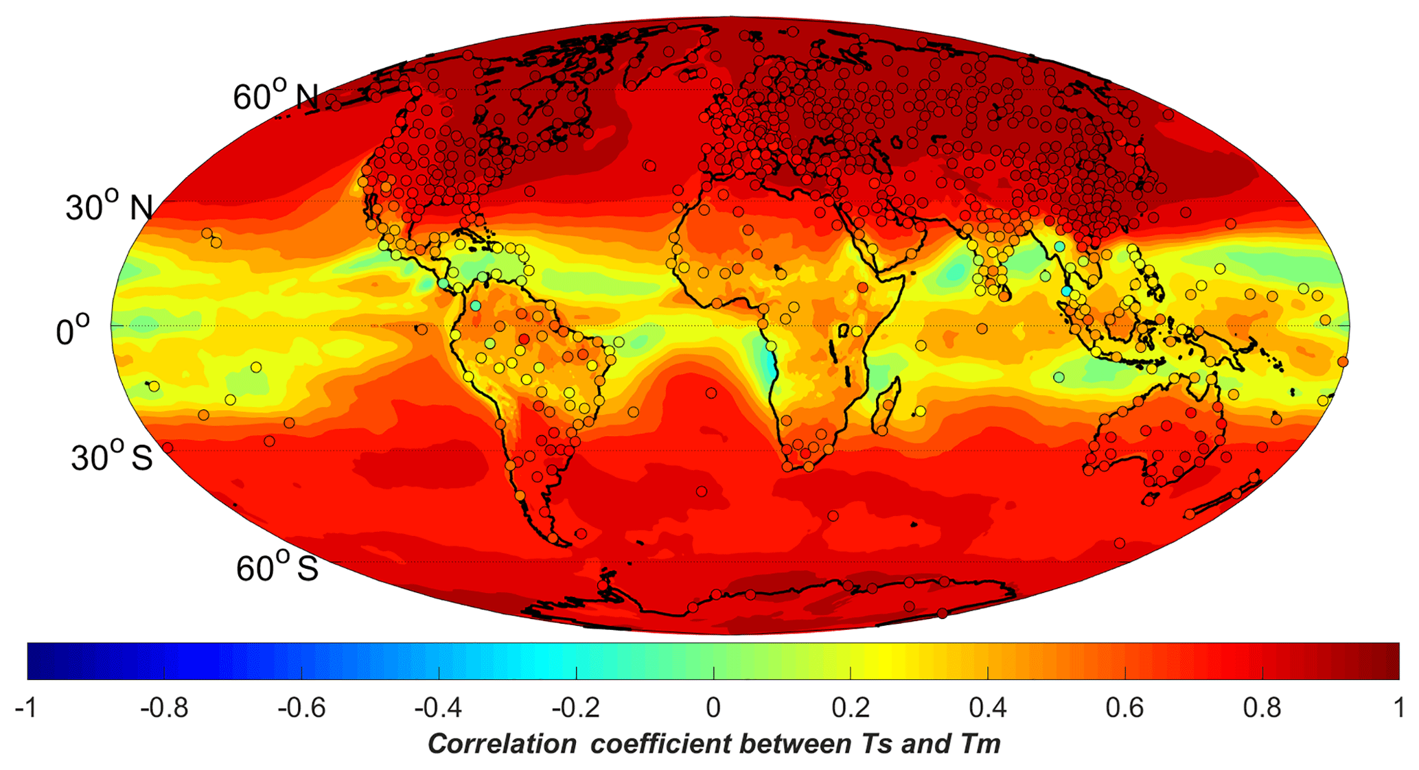
Figure 1Correlation coefficients between Ts and Tm generated from radiosonde data (dots) and ERA-Interim reanalysis data sets (color-filled contours) over a period of 4 years from 2009 to 2012.
We first carried out a linear regression analysis on 4 years of Ts and Tm data generated from the radiosonde data and the global gridded ERA-Interim data sets, with data covering the period January 2009 to December 2012. The analysis results are shown in Fig. 1. Although the two data sets have different temporal resolutions (12 h for the radiosonde data and 6 h for the ERA-Interim data) and spatial resolutions, both analyses agree well with each other. This is expected because the radiosonde data have been assimilated into the ERA-Interim products. Our analyses also indicate that the Ts-=Tm correlation coefficient is generally related to the latitude. The same conclusion has been drawn in other studies (Y. B. Yao et al., 2014). Significant positive correlation coefficients can be found at middle and high latitudes and reach a maximum in the polar regions. The correlation coefficients drop dramatically at low latitudes. This is because Tm is stable there, showing independency of the other parameters. To study the variations of Ts and Tm, we illustrated the denary logarithm values of their standard deviations in Fig. 2. It is evident that Tm varies to a lesser degree than Ts at low latitudes. Aside from the latitude-related features, there are obvious differences of the Ts–Tm correlation coefficients between land and ocean. We even found that negative correlation coefficients over certain oceans, e.g., low-latitude western Pacific, Bay of Bengal or Arabian Sea (see Fig. 1). Unreliable regression analysis results may be derived when the Ts and Tmdata both have small variations. In Fig. 3, scatter plots of Ts and Tm from ERA-Interim at two locations 0.35∘ N 180.00∘ E and 70.53∘ N 180.00∘ E are given. As the blue dots show, the Ts–Tm relationship is weak in the areas near the equator, because the entire variation ranges of Ts and Tm are both within 10 K. This results in a meaningless linear regression (see the magenta line). The Ts–Tm correlation coefficient is only −0.0893 there. Other than the large spatial variations, studies have revealed that the Ts–Tm relationship also has temporal variations (Wang et al., 2005). Therefore, a good Ts–Tm model should take both the spatial and temporal variations into consideration, and this is the main aim in the following sections.
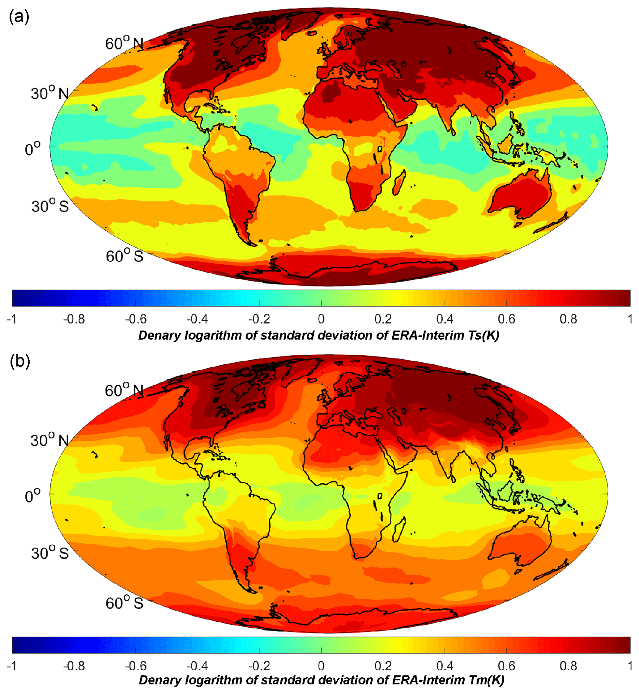
Figure 2Denary logarithm of the standard deviation of (a) Ts and (b) Tm generated from the ERA-Interim data covering the years 2009 to 2012. Temperature unit is Kelvin.
Since the Ts–Tm relationship has large spatial variations, a global gridded Ts–Tm model is preferred for precise GPS–PWV estimations. In this section, a static global gridded model and a time-varying global gridded model are established and assessed.
4.1 Static global-gridded Ts–Tm model
A linear formula for the relation between Tm and Ts has been adopted in many studies. Based on the Ts and Tm products from the ERA-Interim data covering the years 2009 to 2012, we performed linear fittings of Tm versus Ts on each grid point. Then, the slope constant (a), the intercept constant (b) and the fitting root mean square error (RMSE) of each linear expression were calculated and contoured in Fig. 4. The a and b values are related to the latitude as well as the underlying surface (e.g., land, ocean). In the middle–high latitudes over the Northern Hemisphere, constant a value varies from 0.6 to 0.8, and constant b is approximately 100–50 over most of the continents. The constants in the Bevis equation are within these value ranges. Constant a is smaller (approximately 0.5–0.7) over land at the middle–high latitudes over the Southern Hemisphere. In particular, there are abrupt changes in the values of constants a and b from land to ocean at the middle–high latitudes due to the different feature variations of Ts and Tm (see Fig. 2). At low latitudes, the a value is smaller than over the other regions, because of the low variations of Ts and Tm. The fitting RMSEs are within 2–4 K over the middle–high latitude lands, and lower values are obtained over the oceans or at low latitudes. The reason for the low RMSE around the equator is the smaller fluctuation of Tm. Meanwhile, there is no RMSE larger than 4.5 K in the results of our model. As we did not perform any spatial or temporal smoothing of the data during the data processing, both the precision and resolution of our static model are better than other models (e.g., Lan et al., 2016).
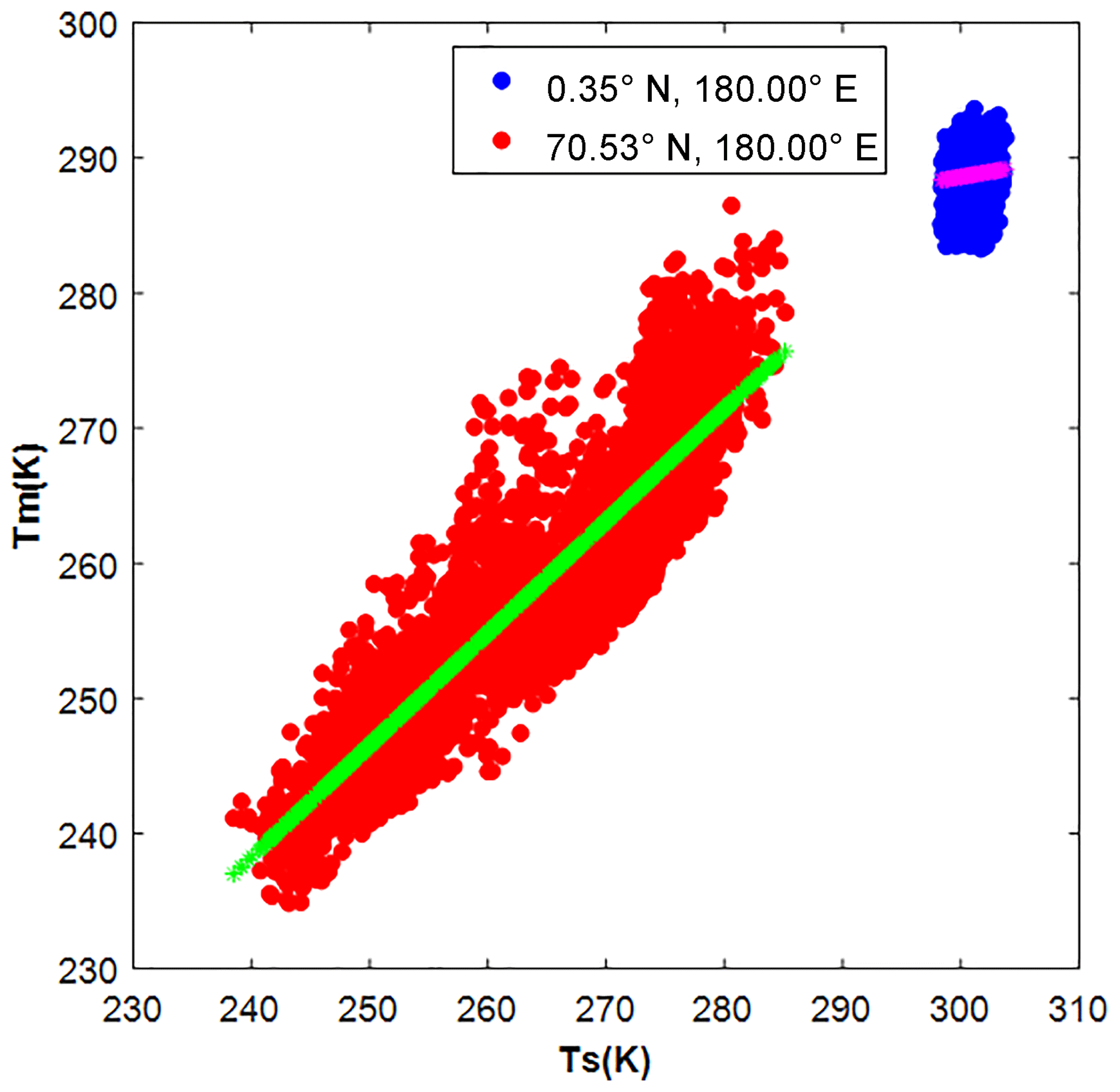
Figure 3Ts–Tm scatter plots at two locations: (blue dots) 0.35∘ N 180.00∘ E and (red dots) 70.53∘ N 180.00∘ E. The magenta and green lines are their linear fitting curves. Temperature unit is Kelvin.
4.2 Time-varying global-gridded Ts–Tm model
The time variation in the Ts–Tm relationship should also be considered in a precise Ts–Tm model. Therefore, a time-varying equation is applied for Ts–Tm regression at each grid node:
where “doy” represents the observed day of year and “h” is the observed hour in UTC time; (m1, m2), (n1, n2) and (p1, p2) are fitting coefficients. These equations can reflect the amplitudes of annual, semiannual and diurnal variations in our Ts–Tm models.
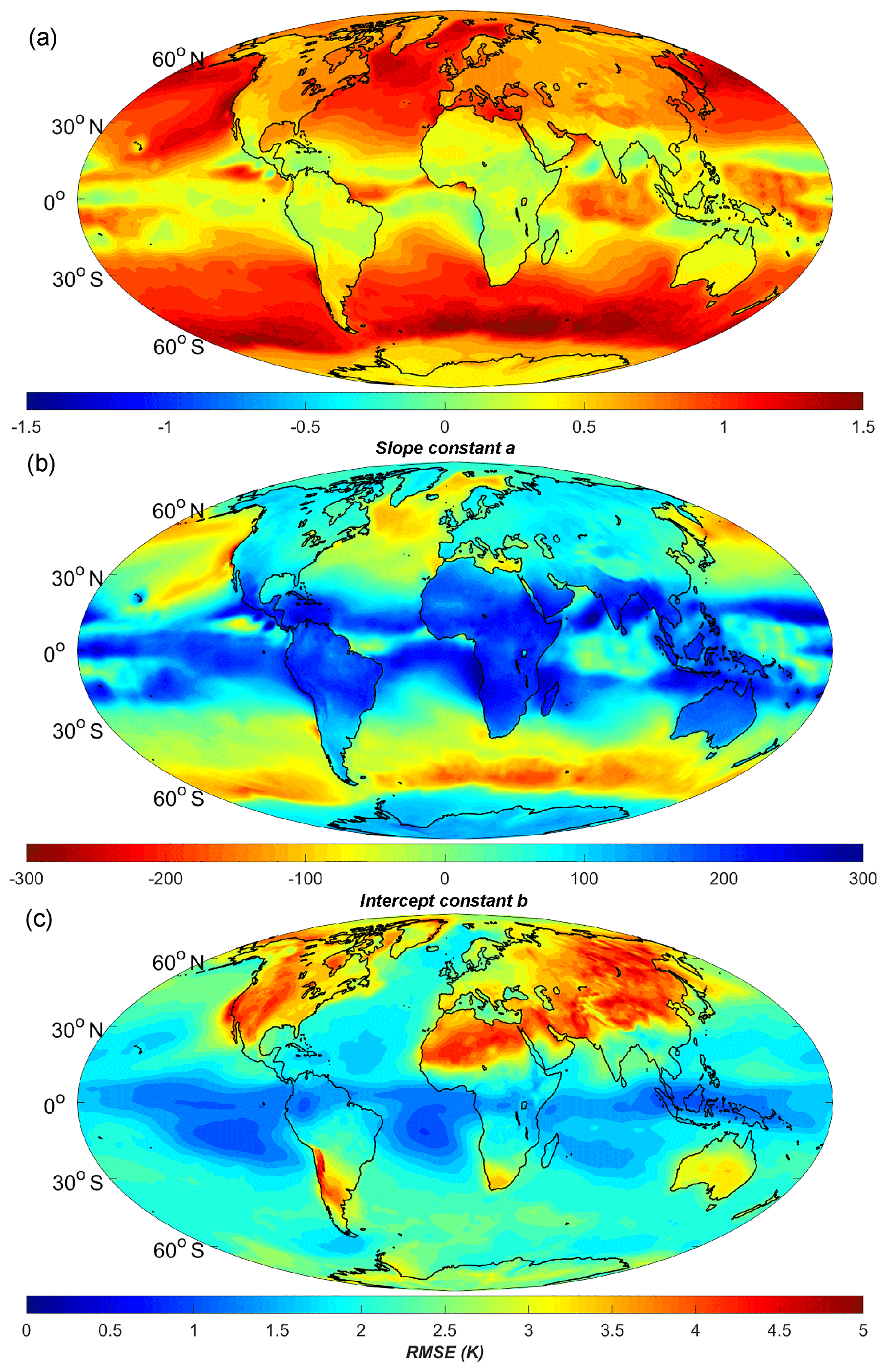
Figure 4Distributions of the (a) slope constant a, (b) intercept constant b and (c) RMSE of static linear Ts–Tm equations at ERA-Interim grid nodes. Temperature unit is Kelvin.
Our new regression model found similar values for the coefficients a and b (of its static term) as for the static model in Sect. 4.1, except for some differences over the oceans. In Fig. 5, besides these constants a and b, we illustrate the amplitudes of annual, semiannual and diurnal terms. We can see that there are large annual variations (amplitude > 5 K) in the vast regions from Tibet to northern Africa, and in some places of the Siberia and Chile. Large diurnal variations (amplitude > 3 K) mainly occur over the midlatitude lands such as northeastern Asia or North America. Semiannual variations, however, are small in most areas except some high-latitude areas (amplitude > 3 K). All variations are smaller over the oceans due to the slower temperature changes over water than over land. The estimated Tm RMSE is also contoured in Fig. 5, and we can see that the RMSE dropped significantly in the regions with large annual or diurnal variations.
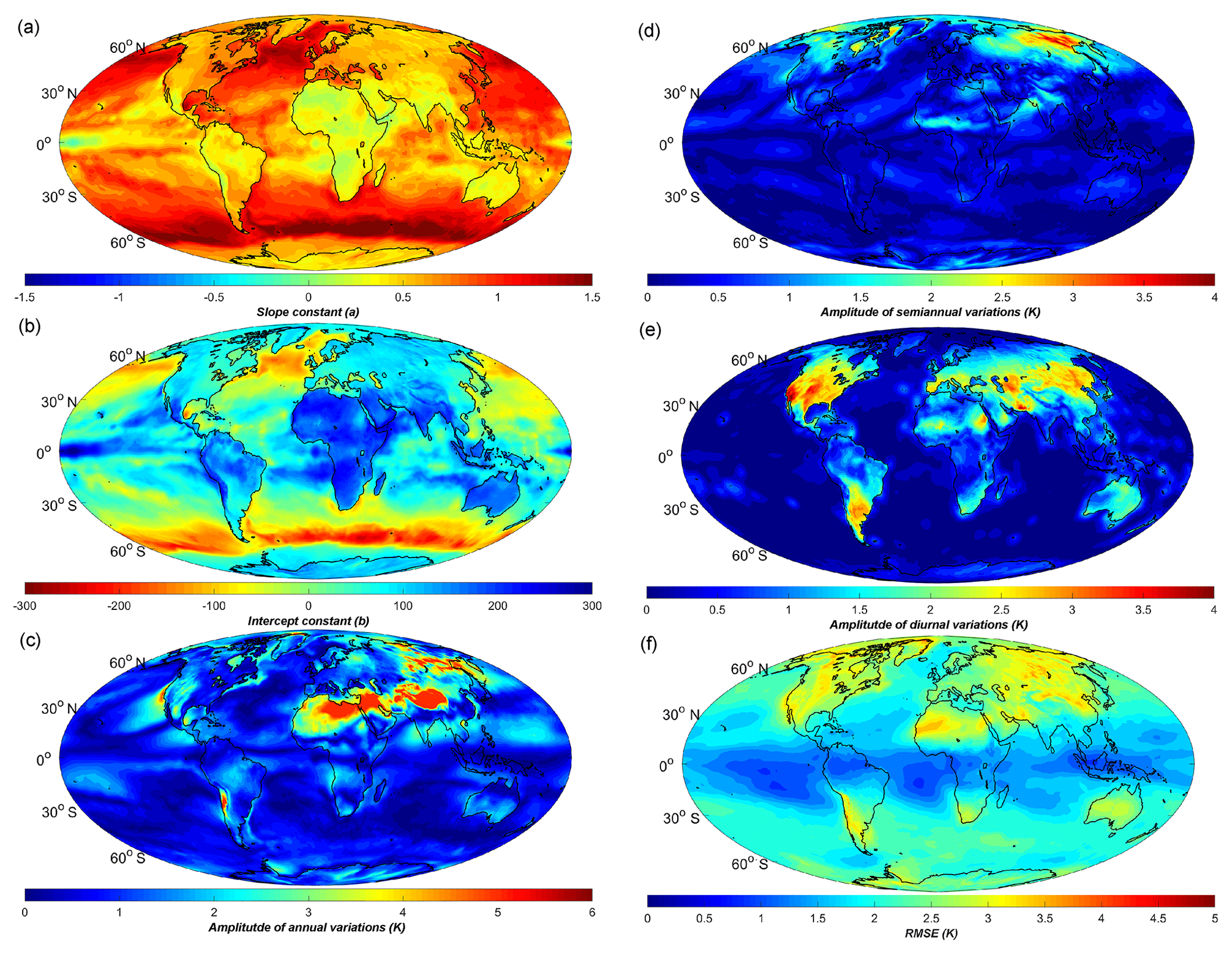
Figure 5(a) The slope constant a, (b) intercept constant b, amplitudes of Tm (c) annual, (d) semiannual and (e) diurnal terms in our time-varying global gridded Ts–Tm model, and (f) the model-estimated Tm RMSE distribution. Temperature unit is Kelvin.
4.3 Assessments of Ts–Tm models
To further assess the precision of the Ts–Tm models using other independent data sources, we generated Tm and Ts from the radiosonde data at 723 radiosonde stations in the year 2016. These data are not assimilated into the 2009–2012 ERA-Interim data sets. As a result, we can regard them to be independent of our model. At each radiosonde site, different Ts–Tm models were employed to calculate Tm. In addition, we also estimated Tm using the 1∘ × 1∘ GPT2w model (Bohm et al., 2015), which is a global gridded Tm empirical model independent of the surface meteorological observation data. Then, these calculated Tm will be evaluated by being compared with the integrated Tm of radiosondes (denoted as Tm_RS) twice a day.
The model estimations of Tm are denoted by Tm_Bevis, Tm_LatR, Tm_static, Tm_varying and Tm_GPT2w for the Bevis equation, the latitude-related model, our static global gridded model, time-varying global gridded model and the GPT2w model. When the global gridded models are employed, the radiosonde station may not be located at a grid node. Therefore, we interpolated the coefficients in the Ts–Tm equations from the neighboring grids to the radiosonde sites. The interpolation formula is expressed as follows (Jade and Vijayan, 2008):
Csite and represent the coefficients in Ts–Tm equations at the radiosonde site location and its neighboring grids, respectively. wi are the interpolation coefficients, which are determined using the equation
where R=6378.17 km is the mean radius of the earth, λ is the scale factor which equals one in our study, and ψi is the angular distance between the ith grid node and the station's position. ψi are computed using following formula (with latitude φ and longitude θ):
Considering the fact that the reanalysis grids are definite and every radiosonde site is in situ, we can compute the interpolation coefficients in Eq. (7) for all of the radiosonde stations. Then, these coefficients are stored as constants to avoid reduplicating the calculation.
Taking Tm_RS as the reference values, we calculated the biases and RMSEs of Tm_Bevis, Tm_LatR, Tm_static, Tm_varying and Tm_GPT2w at each radiosonde site. The results are illustrated in Fig. 6. Obviously, in many regions, the Bevis equation has bad precision with the absolute bias and RMSE both larger than 5 K. Tm_LatR can reduce the estimated biases in many areas, but the RMSEs remain large. Large biases still exist at quite a few radiosonde stations, e.g., in Africa or western Asia. Tm_static and Tm_GPT2w remove the large Tm biases at most of the radiosonde stations. Tm_varying performs significantly better over the world, especially in the Middle East, North America, Siberia, etc.
Detailed statistics of the distributions of the bias and RMSE using different models are shown in Fig. 7 and Table 2. At over 97.37 % of the radiosonde stations, the biases of Tm_varying are within −3–3 K. Large positive biases (>3 K) nearly disappear in Tm_varying. In contrast, there are significant large biases in Tm_Bevis and Tm_LatR. Improvements in RMSE are more evident. The RMSEs of Tm_varying are smaller than 4 K at over 91 % of the radiosonde sites, while few sites (<1 %) have RMSEs larger than 5 K. This is clearly better than the other models. In Tm_Bevis and Tm_LatR, there are more than 17 % of the radiosonde sites with RMSEs larger than 5 K. The overall performance of Tm_GPT2w is very close to Tm_Bevis, except that its absolute bias is smaller than the other Ts–Tm models.
Table 2Statistics of Tm estimates from different models. Reference data are the radiosonde Tm derivations.
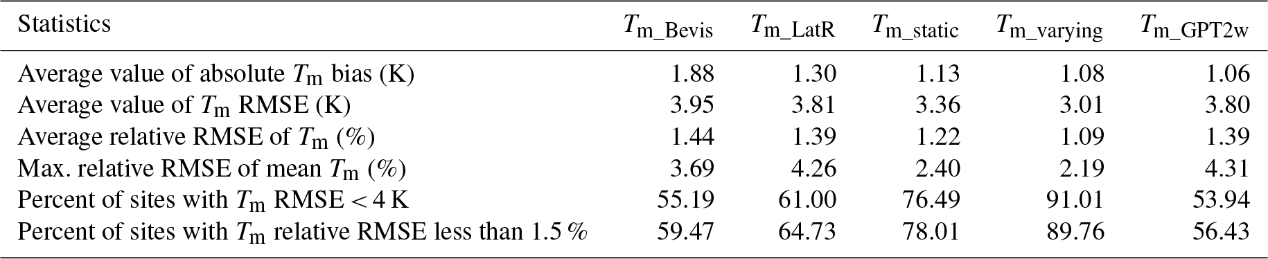
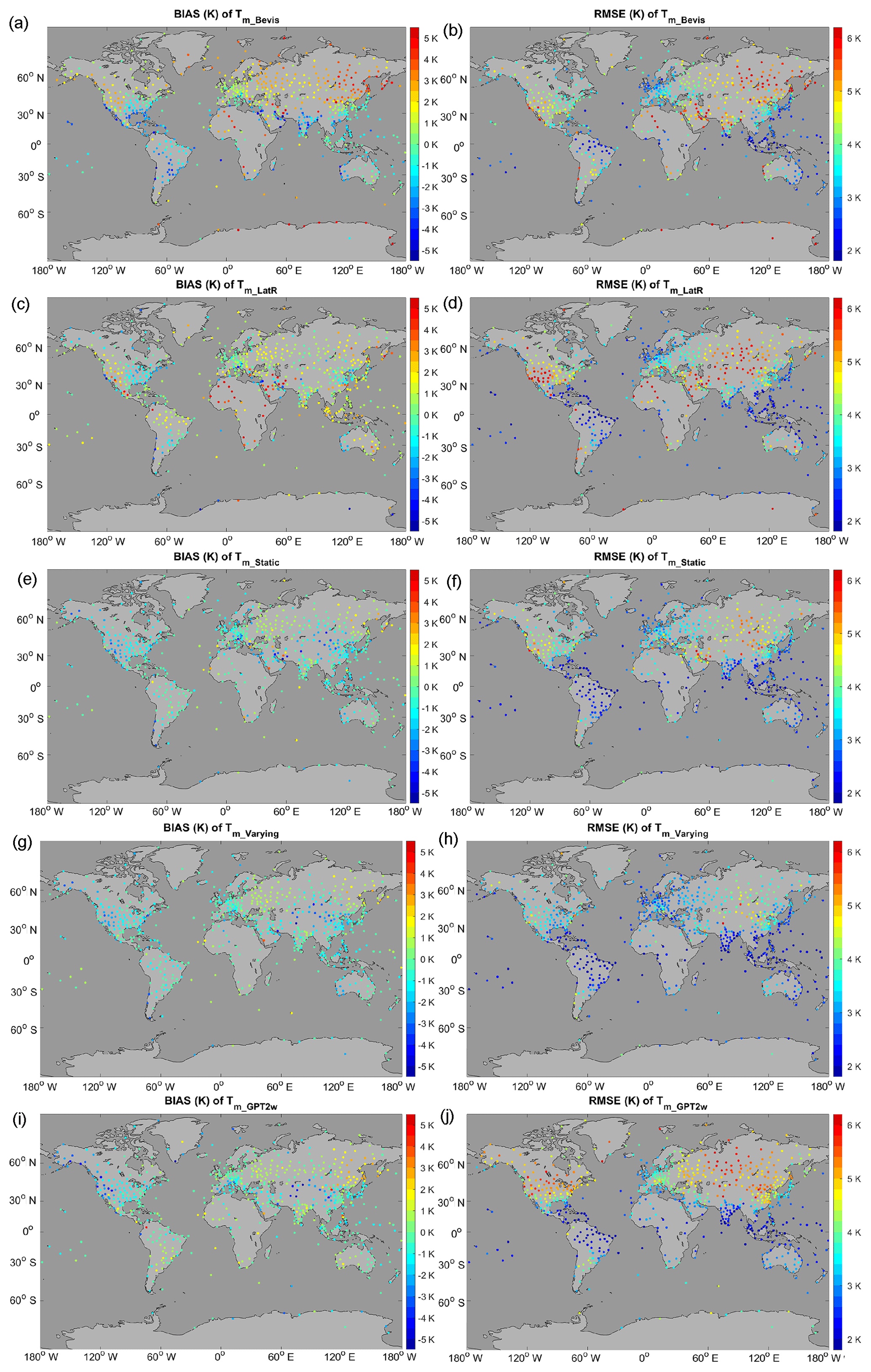
Figure 6(a, c, e, g, i) The biases and (b, d, f, h, j) the RMSEs of the estimated Tm from (a, b) the Bevis equation, (c, d) the latitude-related model, (e, f) our static global gridded model, (g, h) our time-varying global gridded model and (i, j) the GPT2w model at each radiosonde station. Reference data are the radiosonde data of the year 2016. Temperature unit is Kelvin.
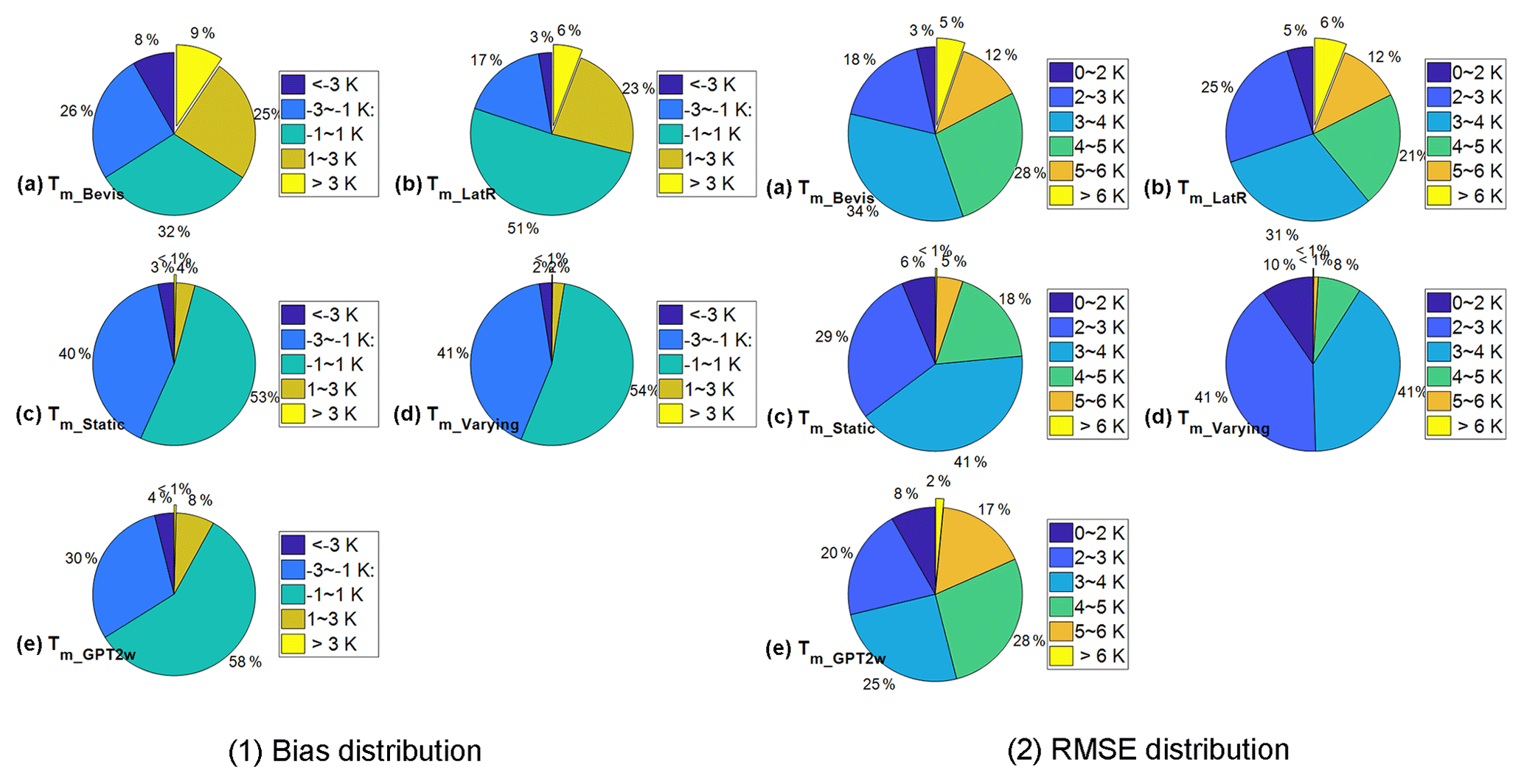
Figure 7The distributions of (1) the biases and (2) the RMSEs of Tm_Bevis, Tm_LatR, Tm_static, Tm_varying and Tm_GPT2w compared with the radiosonde data at 723 stations in the year 2016. Temperature unit is Kelvin.
Table 3Number of radiosonde sites at which the five global applied Tm estimation models had superior performance.
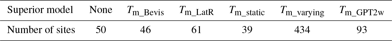
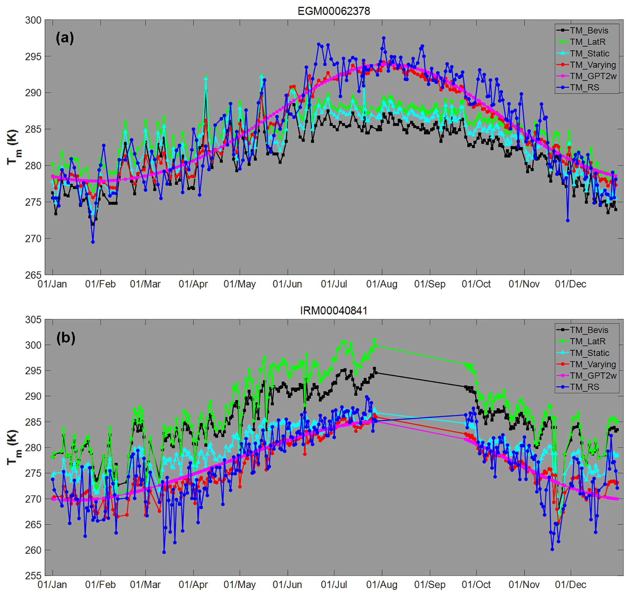
Figure 8Tm series of Tm_Bevis, Tm_LatR, Tm_static, Tm_varying, Tm_GPT2w and Tm_RS at the IGRA station (a) no. 62378 and (b) no. 40841. Temperature unit is Kelvin.
To identify the superior Tm estimation model at each radiosonde site, we employed the following statistical tests under the assumption of a normal distribution of the estimated Tm error:
-
First, Brown–Forsythe tests (Brown and Forsythe, 1974) of the equality of variances were carried out at each site for estimating the Tm errors from two different models, e.g., model A and B. The purpose of this step is to determine whether there are significant differences in the variances of the Tm results. If the test rejects the null hypothesis at a 5 % significance level and the errors of model A and B have the same variance, the model with the smaller sample variance is regarded as the better one. However, if the test does not reject the homogeneity of variances, analysis of variance (ANOVA) is performed in the next step.
-
ANOVA is a technique used to analyze the differences among group means (Hogg and Ledolter, 1987). It evaluates the null hypothesis that the samples all have the same mean against the alternative that the means are not the same. If the null hypothesis is rejected at a 5 % significance level, the Tm sample with smaller absolute mean value is believed to be better. Otherwise, we think that the two models perform almost as well at this radiosonde site.
-
After multiple tests and comparisons, the best model at each radiosonde station may be identified. However, at some sites no superior model can be confirmed. All the models are believed to have equivalent performance.
Finally, we counted the number of sites at which each Tm model performed the best. The results are given in Table 3. The time-varying global gridded model is superior to the others at 434 radiosonde stations (60.03 % of all sites), while the second-best estimation, Tm_GPT2w, is superior at only 12.86 % of the sites.
In Fig. 8 the Tm series at the IGRA station no. 62378 (29.86∘ N 31.34∘ E in Egypt) are given. We can see that large negative biases ( K) between Tm_Bevis (or Tm_LatR) and Tm_RS exist. Tm_static performs only slightly better from July to October. However, Tm_varying and Tm_GPT2w can eliminate most of the seasonal errors. Different properties of Tm series appear at another IGRA station no. 40841 (30.25∘ N 56.97∘ E in Iran). Some observation data are missing, but we can still see that there are large positive differences (>5 K) between Tm_Bevis (or Tm_LatR) and Tm_RS throughout the year. The biases of Tm_static are much smaller, but some large errors still appear in many months. The Tm_varying, however, performs as well as the Tm calculated from the radiosonde data, with small biases, and captures the variations well. The time series ofTm_GPT2w are smoother and cannot capture the fluctuations of the Tm time series, causing an accuracy worse than Tm_varying.
On the other hand, even Tm_varying have large differences from Tm_RS at a few IGRA stations. This can be explained by the fact that our fitting analyses are based on the Tm values derived from ERA-Interim profiles. The quality of ERA-Interim data can be very poor in the regions with sparse observation data (Itterly et al., 2018).
GPS–PWV has different error sources with different properties. It is complicated to evaluate the GPS–PWV uncertainty here due to the lack of collaborated additional independent techniques that monitor water vapor at the GPS site.
5.1 Theoretical analysis of the GPS–PWV uncertainty
Comprehensive research on the uncertainty in GPS–PWV has been carried out by Ning et al. (2016). The uncertainties in ZTD, ZHD and conversion factor Q have been studied in detail. The total uncertainty in GPS–PWV is as follows:
where σPWV, σZTD, and σQ are, respectively, the uncertainties of GPS–PWV, the ZTD estimation, the Ps observations and the conversion factor Q. σc=0.0015 denotes the uncertainty in constant C=2.2767 in Eq. (1), PWV is the value of GPS–PWV, and
where K2 hPa−1, K hPa−1 and , respectively, denote the uncertainties of k3, and Tm in Eq. (4). The variation in σQ with the values of Tm and is depicted in Fig. 9. Assuming that Tm is 280 K, we find that the σQ increases by over 60 % (from 0.069 to 0.112) as the rises from 3.0 to 5.0 K. However, the σQ is less sensitive to the value of Tm. The σQ rises only by 17.96 % (about from 0.061 to 0.075) as the value of Tm drops from 300 to 270 K with K.
Ning et al. (2016) assumed the Tm were obtained from NWP models so the uncertainty in Tm was set to be small ( K). However, as shown in Sect. 4.3, the uncertainties of Tm from different Tm models are significantly larger at the radiosonde stations. For each radiosonde station, we calculated the mean value of Tm and assigned the with the RMSEs of Tm given in Fig. 6. Then we obtained the σQ in Eq. (11). Our statistics indicate that the σQ using our varying Ts–Tm model decreases on average by 19.26 %, 17.77 %, 7.79 % and 18.67 % with respect to the σQ, respectively, using Tm_Bevis, Tm_LatR, Tm_static and Tm_GPT2w. For example, at the IGRA station no. 42724 (22.88∘ N 91.25∘ E in India), σQ drops by 53 % from 0.141 of the Tm_Bevis to 0.066 of the Tm_varying.
The uncertainty in Q will be propagated to the total uncertainty in GPS–PWV according to Eq. (10). We obtained the contributions of the different terms in Eq. (10) to the total GPS–PWV uncertainty. The contribution of one term is measured by the percentage it accounts for the total σPWV. The percentages are computed using the formulas
where pZTD, , pC and pQ, respectively, indicate the contributions of the uncertainties associated with ZTD, Ps, constant C and factor Q to the total σPWV. Following the summaries of Ning et al. (2016), we assumed that σZTD=4 mm and σC=0.0015. Tm identically equals 280 K since the σQ is less sensitive to the value of Tm with respect to the . Table 4 gives five sets of typical values which are assigned to the , , Ps and PWV in Eqs. (10)–(12).
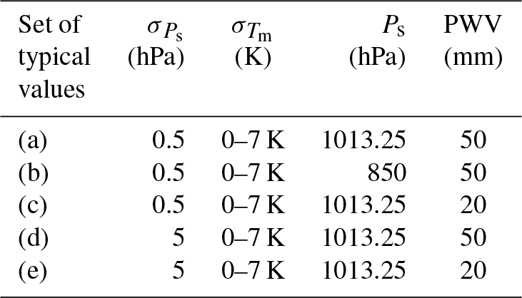
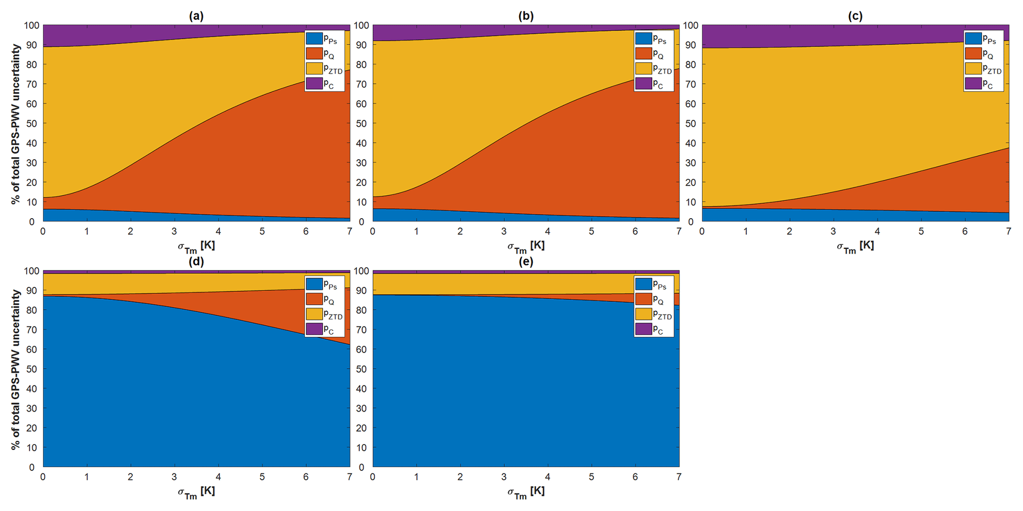
Figure 10Contributions of different terms to the total uncertainty in GPS–PWV with the typical values shown in Table 4.
The equals 0.2 hPa in Ning et al. (2016); however we enlarged its typical value to 0.5 hPa in consideration of the possible worse performance of the surface barometers. In Fig. 10, we illustrated the contributions of the terms in Eq. (12) based on the assumptions (a)–(e) in Table 4. Some feature variations of the contributions of different terms can be found from the comparisons between different subplots:
-
No significant difference exists between Fig. 10a and b. Because of the small value of σc in Eq. (10), the σPWV is not sensitive to the value of Ps. Meanwhile, the uncertainty associated with σc contributes less than 10 % of the σPWV.
-
With the typical values in Table 4 (values a and b), a reduction of can reduce the pQ significantly. For example, in Fig. 10a, the pQ accounts for 69.54 % with K, and it declines to 38.19 % with K.
-
As Fig. 10c shows, the uncertainty associated with σZTD accounts for the main part of σPWV when the values of PWV and are not high. With the typical values in Table 4 (value c), the pZTD can be up to 74.21 % with K. The pQ, however, can drop from 26.76 % to 9.00 % as the decreases from 6 to 3 K. Although the pQ is not large under this situation, a smaller can still reduce the contribution of σQ to the σPWV.
-
The uncertainty associated with dominates the error budget of PWV when the is large. In Fig. 10d and e, the is over 80 % with K and hPa. In Fig. 10d, the pQ increases from 7.55 % to 23.19 % as the rises from 3 to 6 K. However, in Fig. 10e, the pQ only grows from 1.29 % to 4.61 % with the same variation in .
Theoretical analyses of σPWV were also carried out at two representative stations. At the IGRA station no. 42971 (20.25∘ N 85.83∘ E, in India), the mean value of PWV is 53.88 mm. The RMSEs of Tm_Bevis, Tm_LatR, Tm_static, Tm_varying and Tm_GPT2w are 4.30, 3.15, 2.41, 1.93 and 1.97 K. The in Eq. (11) was replaced by the calculated RMSEs, and the pZTD, , pC and pQ were generated with two typical values, 0.5 and 5 hPa, assigned to the . With hPa, the pC accounts for around 7 %, while the accounts for around 4 % of the total σPWV. By using different Tm estimations, the variations of pC and are both within 4 %. However, the pQ varies more evidently. It accounts for averages of 55.69 %, 40.77 %, 30.70 %, 23.53 % and 24.11 % of the σPWV with the estimations of Tm_Bevis, Tm_LatR, Tm_static, Tm_varying and Tm_GPT2w, respectively. The pZTD rises with the reduction of pQ, e.g., from 36.23 % of Tm_Bevis to 62.53 % of Tm_varying. On the other hand, with hPa, the accounts for more than 75 % of the σPWV, while the pQ decreases from 14.21 % of Tm_Bevis to 3.9 % of Tm_varying.
At another representative station, the IGRA station no. 50557 (49.17∘ N 125.22∘ E, in northeastern China), the mean PWV is only 12.17 mm. The RMSEs of Tm_Bevis, Tm_LatR, Tm_static, Tm_varying and Tm_GPT2w are 5.16, 3.94, 3.54, 2.99 and 5.10 K. We can see that the accuracy of Tm has been improved significantly. However, because of the low average value of PWV, the pZTD averagely contributes over 73.5 % of the σPWV, while the pQ averagely contributes less than 10.5 % assuming hPa and less than 1.5 % assuming hPa. But such a discussion only concerns the average values. In fact, even at this station there are still some high values of PWV, for example at 12:00 UTC 22 July 2016, the PWV reached 48 mm. For the observations with high PWV, the improvement in the accuracy of Tm can still exert a significant positive impact on the reduction of pQ.
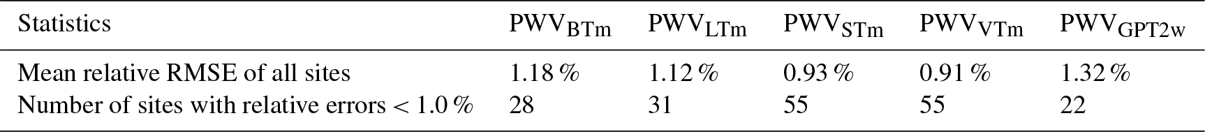
Table 5Statistics on the relative errors of different PWV retrievals.
It is worth mentioning that the uncertainty in ZHD may be underestimated in some situations. There are two reasons for this. Firstly, the calculation of ZHD assumes that the water vapor does not contribute to the mass of the atmosphere. The ZHD error introduced by this assumption is often negligible. But in some very wet regions, the mass of water vapor could produce significant errors in the ZHD calculation. Secondly, and more importantly, the error of Ps in Eq. (1) can sometimes be very large. Small is reasonable when the surface barometer is calibrated routinely and equipped together with the GPS antenna. However, if there were significant height difference between the GPS antenna and the barometer, the error for ZHD would increase significantly. Snajdrova et al. (2006) found that 10 m of height difference approximately causes a difference of 3 mm in the ZHD. On the other hand, Ps can be generated from NWP data if there are no nearby barometers at GPS site. The error of Ps could be very large using this method (Means and Cayan, 2013; Jiang et al., 2016). In these cases, the GPS–PWV error reduction will be very limited due to the more precise Tm estimation.
5.2 Impact of real Tm estimation
To study the impact of Tm on the real GPS–PWV retrieval, we first downloaded GPS ZTD products (Byun and Bar-Sever, 2009) at 74 IGS sites in the year 2016 from the NASA Crustal Dynamics Data Information System (CDDIS) ftp address (ftp://cddis.gsfc.nasa.gov/pub/gps/products/troposphere/zpd, last access: 25 February 2019). These selected GPS sites were equipped with meteorological sensors so that the surface pressure and temperature measurements could also be obtained. ZHD was calculated using Eq. (1). It is subtracted from ZTD to obtain ZWD. Then, Tm was generated with six approaches: the first five Tm series were Tm_Bevis, Tm_LatR, Tm_static, Tm_varying and Tm_GPT2w. The sixth Tm was integrated from the ERA-Interim profiles and interpolated to each GPS site (Jiang et al., 2016; Wang et al., 2016). Finally, the GPS–PWV was generated from the ZWD and the six different Tm estimates leading to over 100 compared points for each GPS–PWV series. We denoted these GPS–PWV sets as PWVBTm, PWVLTm, PWVSTm, PWVVTm, PWVGTm and PWVETm. The only difference between these GPS and PWV estimations is the Tm estimation model; therefore, the impact of other errors is excluded.
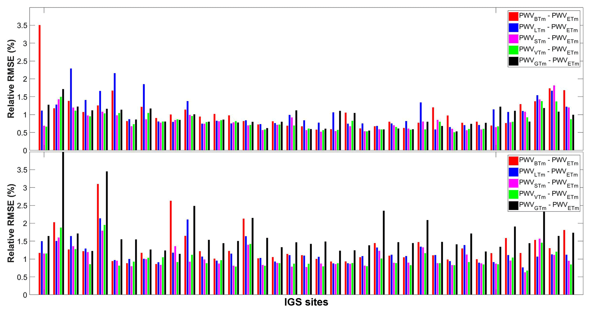
Figure 11Relative RMSEs of PWVBTm, PWVSTm, PWVVTm and PWVGTm compared with PWVETm at 74 IGS stations in the year 2016.
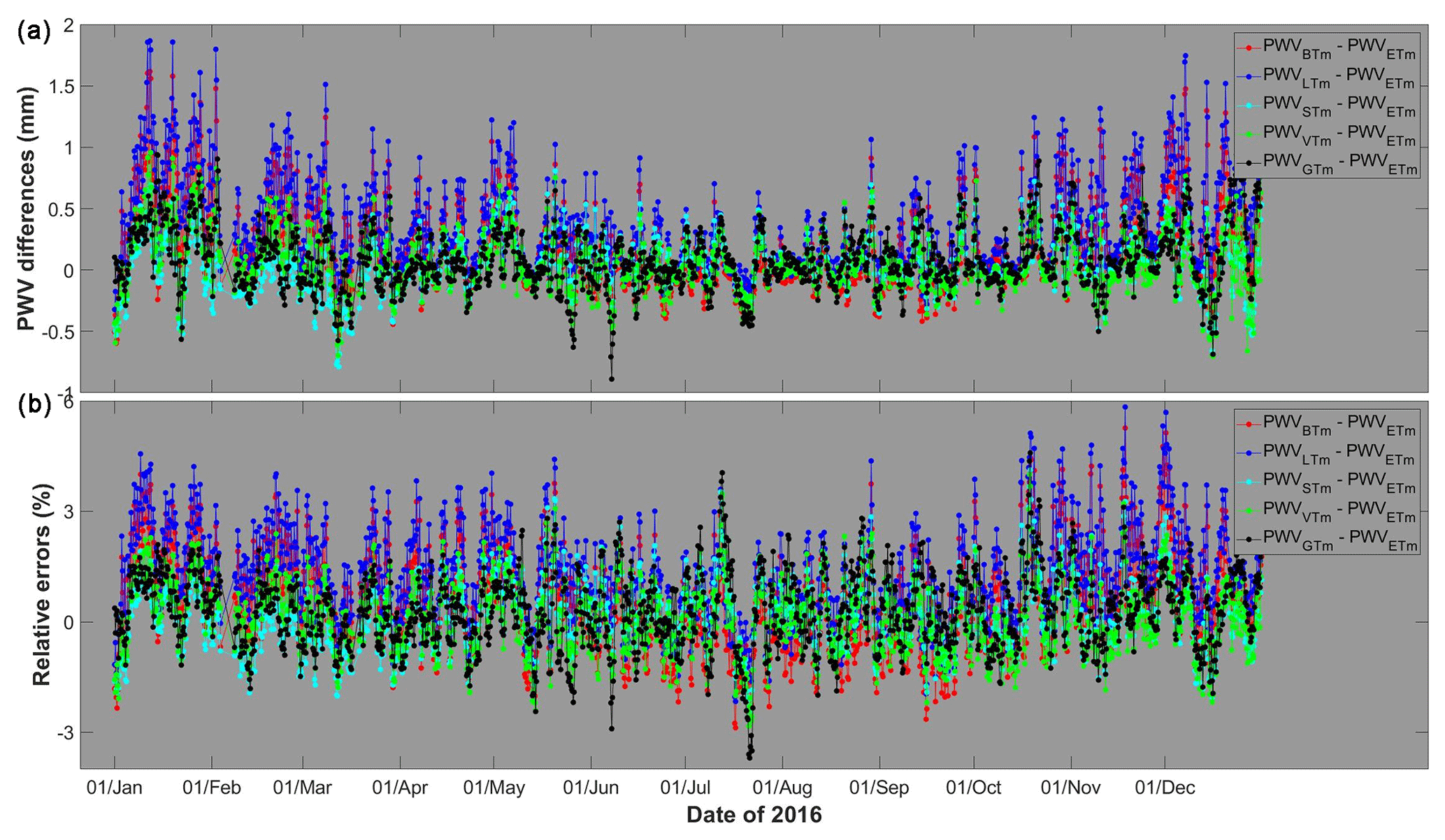
Figure 12(a) PWV differences and (b) relative differences of PWVBTm, PWVLTm, PWVSTm, PWVVTM and PWVGTm compared with PWVETm at the ALIC station in the year 2016. PWV unit is millimeters.
The Tm from ERA-Interim is believed to be the most accurate among our Tm estimates at the selected GPS sites. We therefore took the PWVETm as reference values to assess the other PWV. The relative RMSEs of PWVBTm, PWVLTm, PWVSTm, PWVVTm and PWVGTm at these selected stations were calculated and are illustrated in Fig. 11. Detailed statistics are given in Table 5. The mean relative error of all sites drops from 1.18 % of the PWVBTm to 0.91 % of the PWVVTm. PWVVTm has the minimum mean relative errors at 51.35 % of the sites, while PWVSTm is superior at 27.03 % of the sites. PWVSTm and PWVVTm obtain relative RMSEs smaller than 1.0 % at 55 sites, while only 28 sites of PWVBTm, 31 sites of PWVLTm and 22 sites of PWVGTm perform similarly. For example, at the ALIC site (23.67∘ S 133.89∘ E, in Australia), with a mean PWV of approximately 23 mm, the relative RMSE dropped from 1.97 % of PWVBTm to 1.10 % of PWVVTm. The time series of the relative differences of PWVBTm, PWVLTm, PWVSTm, PWVVTm and PWVGTm are given in Fig. 12. We found that some relative RMSEs could be reduced by more than 2 % from PWVBTm to PWVVTm. Obviously, PWVBTm and PWVLTm have larger relative errors throughout the year, while the PWV differences are significantly larger only in the summer season (when the PWV values are highest). Apparently, the Tm variations in summer are not modeled well by either the Bevis model and the latitude-related model. PWVSTm eliminate those large differences but still retain some residual errors, which are removed by more than 0.5 mm in PWVVTm. PWVGTm has some large errors during the period from May to July. All of these results demonstrate that our time-varying model has a precision advantage.
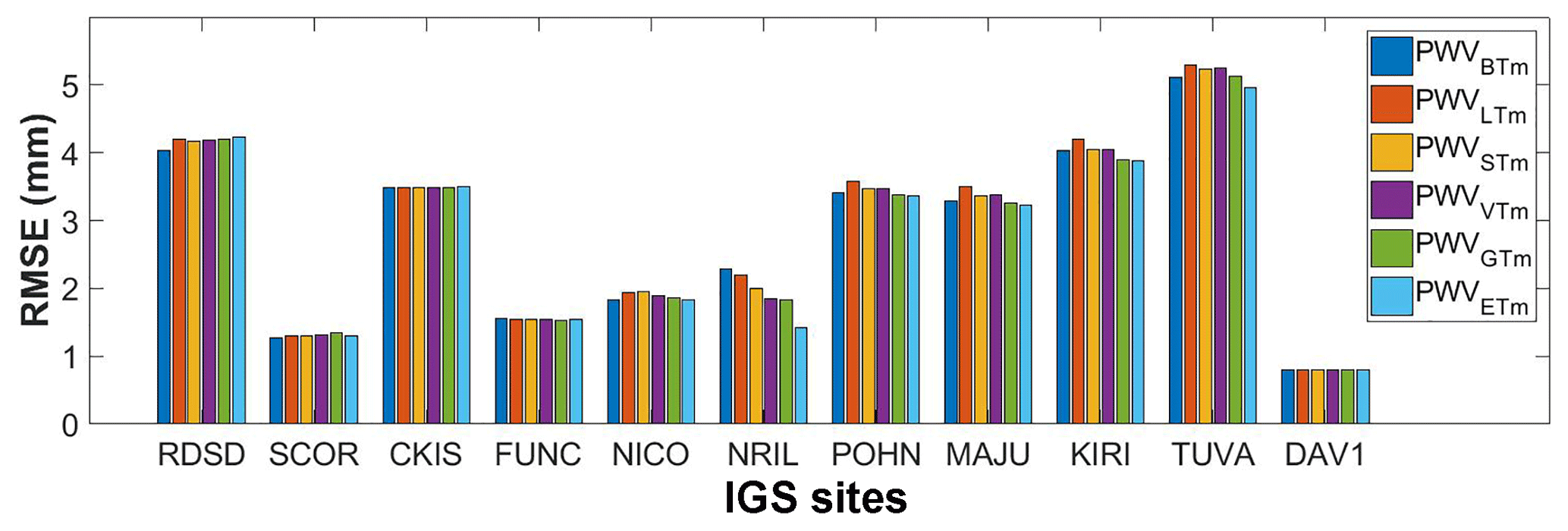
Figure 13RMSEs of the PWVBTm, PWVSTm, PWVVTm, PWVGTm and PWVETm compared with the PWVRS at 11 IGS stations in 2016. PWV unit is millimeters.
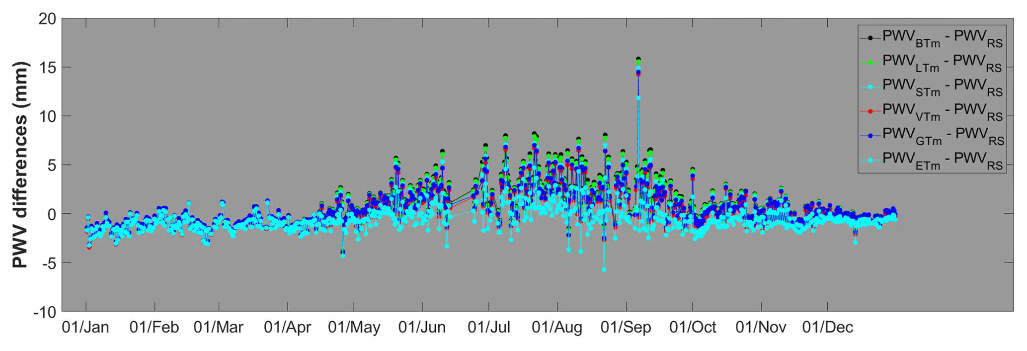
Figure 14PWV differences of the PWVBTm, PWVLTm, PWVSTm, PWVVTm, PWVGTm and PWVETm compared with the PWVRS at the NIRL station in the year 2016. PWV unit is millimeters.
5.3 Comparisons between GPS–PWV and radiosonde PWV
Among our selected 74 IGS sites, there are only 11 sites located within 5 km to a nearby IGRA radiosonde station. At these common stations, we generated PWV from the radiosonde data (PWVRS) by adjusting the sounding profiles to the heights of IGS sites. It is worth noting that a geoid undulation correction should be carried out on each IGS site geoid height (Jiang et al., 2016). Then, we compared PWVBTm, PWVLTm, PWVSTm, PWVVTm, PWVGTm and PWVETm with PWVRS. Figure 13 shows the statistics. The RMSEs of GPS–PWV are approximately 1–5 mm. Comparisons indicate that the RMSEs of different GPS–PWV retrievals are very close (differences < 0.2 mm) regardless of the applied Tm sources at most of the selected sites. This means that other errors (e.g., ZTD estimation errors or sounding sensors errors) instead of the Tm make up the bulk of the differences between the GPS–PWV and the radiosonde PWV. Actually, each sounding does not represent the vertical sounding centered at the radiosonde site because of the complex path of the balloon. And GPS–PWV represents the averaged value of the water vapor zenithal projection from all the slant signal paths during the observation period. Such differences can introduce significant uncertainty into our comparisons. However, we still found obvious gaps between PWV at the NRIL station (88.36∘ N 69.36∘ E, 4.1 km away from the IGRA station no. 23078 in Russia). The RMSE decreases from 2.29 mm of PWVBTm to 1.84 mm of PWVVTm and 1.42 mm of PWVETm. As shown in Fig. 14, the large PWV differences appear mainly from May to September. During those five months, the mean GPS–PWV difference to PWVRS decreases by over 30 % from 2.52 mm of PWVBTm to 1.67 mm of PWVVTm, and the reductions of GPS–PWV error are mainly around 1–2 mm. This is attributed to the wetter atmosphere in these months. As indicated by the uncertainty analysis in Sect. 5.1, the improvement in the accuracy of Tm can be translated into more error reduction in the GPS–PWV retrieval with higher values of PWV.
We developed two global gridded Ts–Tm models, which are, respectively, static and time-varying with a spatial resolution of 0.75∘ × 0.75∘. The models are established by analyzing the ERA-Interim reanalysis data sets covering the years 2009–2012, which indicated the significant spatial–temporal variations in Ts–Tm relationship as well as the radiosondes covering the same period. The annual, semiannual and diurnal variations in Ts–Tm relationship are considered in the time-varying model. The time-varying global gridded Ts–Tm model has a significant global precision advantage over the other globally applied models, including the Bevis equation, the latitude-related model and the GPT2w model. The average RMSE of Tm reduces by approximately 1 K. At over 90 % of the radiosonde sites, our time-varying model has RMSE smaller than 4 K, while the RMSEs larger than 5 K nearly disappear. On the other hand, in the Bevis model or in the latitude-related model, there are more than 17 % of the radiosonde sites with RMSEs larger than 5 K. Multiple statistical tests at the 5 % significance level identified the significant superiority of our varying model at more than 60 % of the radiosonde sites. Analyses at the specific stations demonstrate that the errors larger than 5 K in the estimated Tm series can be eliminated by our varying Ts–Tm model.
More precise Tm estimations can decrease by around 20 % of the uncertainty in the conversion factor Q, which maps GPS–ZWD to GPS–PWV, and the reduction can be even more than 50 % at some stations. The contribution of the uncertainty associated with Q to the total GPS–PWV uncertainty also declines when using a more precise Tm model. The reduction is related to the value of PWV and the uncertainty in the surface pressure. With GPS–PWV higher than 50 mm, the uncertainty associated with Q contributes more than 55 % of the uncertainty in GPS–PWV when using the Bevis equation and less than 25 % when using our varying Ts–Tm model, assuming the ZTD and the surface pressure are measured accurately with the uncertainties of 4 mm and 0.5 hPa, respectively. However, the uncertainty in ZTD or in surface pressure would dominate the error budget of GPS–PWV (>70 %) if the value of GPS–PWV were small or the uncertainty in surface pressure were large. In these cases, the uncertainty associated with Q only contributes around 10 % of the GPS–PWV uncertainty or even smaller. Taking the GPS–PWV, using ERA-Interim Tm estimates at 74 IGS sites as the references, we found that the GPS–PWV using our time-varying Ts–Tm model obtained the minimum mean relative error at 51.35 % of the sites, while the GPS–PWV using the static gridded Ts–Tm model is superior at only 27.03 % of the sites. The differences between GPS–PWV and radiosonde PWV are approximately 1–5 mm. And our varying Ts–Tm model can reduce the error in the GPS–PWV retrieval by 30 % (around 1–2 mm) with respect to the Bevis equation.
According to our experiments, we are confident that the time-varying global gridded Ts–Tm models presented here will help us to retrieve GPS PWV more precisely and to study the precise PWV variations in high temporal resolution. The Matlab array file consisting of the global gridded coefficients in our model, as well as codes for interpolating coefficients at any given location, is provided in the supplement of this study.
-
Radiosonde data: ftp://ftp.ncdc.noaa.gov/pub/data/igra (IGRA radiosonde data, 2019);
-
ERA-Interim project: https://doi.org/10.5065/D6CR5RD9 (European Centre for Medium-Range Weather Forecasts, 2019);
-
GPS-ZTD product: ftp://cddis.gsfc.nasa.gov/pub/gps/products/troposphere/zpd (CDDIS GPS-ZTD Product, 2019).
The supplement related to this article is available online at: https://doi.org/10.5194/amt-12-1233-2019-supplement.
PJ, SY and YW conceived and designed the experiments; PJ, YL performed the experiments and analyzed the results; and DC and YL processed the data. All authors contributed to the writing of the paper.
The authors declare that they have no conflict of interest.
This study is supported by the National Natural Science Foundation of China
(no. 41604028), the Anhui Provincial Natural Science Foundation (no. 1708085QD83),
and the Doctoral Research Start-up Funds Projects of Anhui University (no. J01001966).
The authors thank the European Centre for Medium-Range Weather Forecasts for
providing the ERA-Interim data set. We also thank the National Centers for
Environmental Information for the IGRA data sets and International GNSS Service
for the GNSS troposphere products.
Edited by: Roeland Van Malderen
Reviewed by: David Adams and four anonymous referees
Adams, D. K., Barbosa, H. M. J., and De Los Rios, K. P. G.: A Spatiotemporal Water Vapor-Deep Convection Correlation Metric Derived from the Amazon Dense GNSS Meteorological Network, Mon. Weather Rev., 145, 279–288, https://doi.org/10.1175/mwr-d-16-0140.1, 2017.
Adler, B., Kalthoff, N., Kohler, M., Handwerker, J., Wieser, A., Corsmeier, U., Kottmeier, C., Lambert, D., and Bock, O.: The variability of water vapour and pre-convective conditions over the mountainous island of Corsica, Q. J. Roy. Meteorol. Soc., 142, 335–346, https://doi.org/10.1002/qj.2545, 2016.
Bevis, M., Businger, S., Herring, T. A., Rocken, C., Anthes, R. A., and Ware, R. H.: GPS meteorology: Remote sensing of atmospheric water vapor using the global positioning system, J. Geophys. Res.-Atmos., 97, 15787–15801, https://doi.org/10.1029/92JD01517, 1992.
Bohm, J., Moller, G., Schindelegger, M., Pain, G., and Weber, R.: Development of an improved empirical model for slant delays in the troposphere (GPT2w), GPS Solutions, 19, 433–441, https://doi.org/10.1007/s10291-014-0403-7, 2015.
Brown, M. B. and Forsythe, A. B.: Robust Tests for the Equality of Variances, Publ. Am. Stat. Assoc., 69, 364–367, 1974.
Byun, S. H. and Bar-Sever, Y. E.: A new type of troposphere zenith path delay product of the international GNSS service, J. Geodesy, 83, 367–373, https://doi.org/10.1007/s00190-008-0288-8, 2009.
Campmany, E., Bech, J., Rodriguez-Marcos, J., Sola, Y., and Lorente, J.: A comparison of total precipitable water measurements from radiosonde and sunphotometers, Atmosp. Res., 97, 385–392, https://doi.org/10.1016/j.atmosres.2010.04.016, 2010.
CDDIS GPS-ZTD Product: ftp://cddis.gsfc.nasa.gov/pub/gps/products/troposphere/zpd, last access: 26 February 2019.
Chen, P., Yao, W. Q., and Zhu, X. J.: Realization of global empirical model for mapping zenith wet delays onto precipitable water using NCEP re-analysis data, Geophys. J. Int., 198, 1748–1757, https://doi.org/10.1093/gji/ggu223, 2014.
Ciesielski, P. E., Chang, W. M., Huang, S. C., Johnson, R. H., Jou, B. J. D., Lee, W. C., Lin, P. H., Liu, C. H., and Wang, J. H.: Quality-Controlled Upper-Air Sounding Dataset for TiMREX/SoWMEX: Development and Corrections, J. Atmos. Ocean. Tech., 27, 1802–1821, https://doi.org/10.1175/2010jtecha1481.1, 2010.
European Centre for Medium-Range Weather Forecasts: ERA-Interim Project, Research Data Archive at the National Center for Atmospheric Research, Computational and Information Systems Laboratory, https://doi.org/10.5065/D6CR5RD9, 2019.
Haase, J., Ge, M., Vedel, H., and Calais, E.: Accuracy and variability of GPS tropospheric delay measurements of water vapor in the western Mediterranean, J. Appl. Meteorol., 42, 1547–1568, https://doi.org/10.1175/1520-0450(2003)042<1547:AAVOGT>2.0.CO;2, 2003.
Hogg, R. V. and Ledolter, J.: Enginering Statistics, Macmillan, New York, 1987.
IGRA radiosonde data: https://www1.ncdc.noaa.gov/pub/data/igra/, last access: 26 Februray 2019.
Itterly, K. F., Taylor, P. C., and Dodson, J. B.: Sensitivity of the Amazonian Convective Diurnal Cycle to Its Environment in Observations and Reanalysis, J. Geophys. Res.-Atmos., 23, 12621–12646, https://doi.org/10.1029/2018JD029251, 2018.
Jade, S. and Vijayan, M. S. M.: GPS-based atmospheric precipitable water vapor estimation using meteorological parameters interpolated from NCEP global reanalysis data, J. Geophys. Res.-Atmos., 113, D03106, https://doi.org/10.1029/2007jd008758, 2008.
Jiang, P., Ye, S. R., Chen, D. Z., Liu, Y. Y., and Xia, P. F.: Retrieving Precipitable Water Vapor Data Using GPS Zenith Delays and Global Reanalysis Data in China, Remote Sensing, 8, 389, https://doi.org/10.3390/rs8050389, 2016.
Karabatic, A., Weber, R., and Haiden, T.: Near real-time estimation of tropospheric water vapour content from ground based GNSS data and its potential contribution to weather now-casting in Austria, Adv. Space Res., 47, 1691–1703, https://doi.org/10.1016/j.asr.2010.10.028, 2011.
Kealy, J., Foster, J., and Businger, S.: GPS meteorology: An investigation of ocean-based precipitable water estimates, J. Geophys. Res.-Atmos., 117, D17303, https://doi.org/10.1029/2011jd017422, 2012.
Lan, Z., Zhang, B., and Geng, Y.: Establishment and analysis of global gridded Tm–Ts relationship model, Geodesy Geodynam., 7, 101–107, https://doi.org/10.1016/j.geog.2016.02.001, 2016.
Lee, J., Park, J.-U., Cho, J., Baek, J., and Kim, H. W.: A characteristic analysis of fog using GPS-derived integrated water vapour, Meteorol. Appl., 17, 463–473, https://doi.org/10.1002/met.182, 2010.
Li, X., Zhang, L., Cao, X. J., Quan, J. N., Wang, T. H., Liang, J. N., and Shi, J. S.: Retrieval of precipitable water vapor using MFRSR and comparison with other multisensors over the semi-arid area of northwest China, Atmos. Res., 172, 83–94, https://doi.org/10.1016/j.atmosres.2015.12.015, 2016.
Liu, Z. Z., Li, M., Zhong, W. K., and Wong, M. S.: An approach to evaluate the absolute accuracy of WVR water vapor measurements inferred from multiple water vapor techniques, J. Geodynam., 72, 86–94, https://doi.org/10.1016/j.jog.2013.09.002, 2013.
Lu, C. X., Li, X. X., Nilsson, T., Ning, T., Heinkelmann, R., Ge, M. R., Glaser, S., and Schuh, H.: Real-time retrieval of precipitable water vapor from GPS and BeiDou observations, J. Geodesy, 89, 843–856, https://doi.org/10.1007/s00190-015-0818-0, 2015.
Mahoney, K., Jackson, D. L., Neiman, P., Hughes, M., Darby, L., Wick, G., White, A., Sukovich, E., and Cifelli, R.: Understanding the role of atmospheric rivers in heavy precipitation in the Southeast US, Mon. Weather Rev., 144, 1617–1632, https://doi.org/10.1175/MWR-D-15-0279.1, 2016.
Means, J. D.: GPS Precipitable Water as a Diagnostic of the North American Monsoon in California and Nevada, J. Climate, 26, 1432–1444, https://doi.org/10.1175/jcli-d-12-00185.1, 2013.
Means, J. D. and Cayan, D.: Precipitable Water from GPS Zenith Delays Using North American Regional Reanalysis Meteorology, J. Atmos. Ocean. Tech., 30, 485–495, https://doi.org/10.1175/jtech-d-12-00064.1, 2013.
Ning, T., Elgered, G., Willen, U., and Johansson, J. M.: Evaluation of the atmospheric water vapor content in a regional climate model using ground-based GPS measurements, J. Geophys. Res.-Atmos., 118, 329–339, https://doi.org/10.1029/2012jd018053, 2013.
Ning, T., Wang, J., Elgered, G., Dick, G., Wickert, J., Bradke, M., Sommer, M., Querel, R., and Smale, D.: The uncertainty of the atmospheric integrated water vapour estimated from GNSS observations, Atmos. Meas. Tech., 9, 79–92, https://doi.org/10.5194/amt-9-79-2016, 2016.
Pacione, R. and Vespe, F.: Comparative studies for the assessment of the quality of near-real-time GPS-derived atmospheric parameters, J. Atmos. Ocean. Tech., 25, 701–714, https://doi.org/10.1175/2007jtecha935.1, 2008.
Perez-Ramirez, D., Whiteman, D. N., Smirnov, A., Lyamani, H., Holben, B. N., Pinker, R., Andrade, M., and Alados-Arboledas, L.: Evaluation of AERONET precipitable water vapor versus microwave radiometry, GPS, and radiosondes at ARM sites, J. Geophys. Res.-Atmos., 119, 9596–9613, https://doi.org/10.1002/2014jd021730, 2014.
Rocken, C., Johnson, J., Van Hove, T., and Iwabuchi, T.: Atmospheric water vapor and geoid measurements in the open ocean with GPS, Geophys. Res. Lett., 32, L12813, https://doi.org/10.1029/2005gl022573, 2005.
Rohm, W., Yuan, Y. B., Biadeglgne, B., Zhang, K. F., and Le Marshall, J.: Ground-based GNSS ZTD/IWV estimation system for numerical weather prediction in challenging weather conditions, Atmos. Res., 138, 414–426, https://doi.org/10.1016/j.atmosres.2013.11.026, 2014.
Sheng, P., Mao, J., Li, J., Ge, Z., Zhang, A., Sang, J., Pan, N., and Zhang, H.: Atmospheric Physics, 2nd Edn., Peking University Press, Beijing, 2013.
Singh, D., Ghosh, J. K., and Kashyap, D.: Weighted mean temperature model for extra tropical region of India, J. Atmos. Sol.-Terr. Phys., 107, 48–53, https://doi.org/10.1016/j.jastp.2013.10.016, 2014.
Snajdrova, K., Boehm, J., Willis, P., Haas, R., and Schuh, H.: Multi-technique comparison of tropospheric zenith delays derived during the CONT02 campaign, J. Geodesy, 79, 613–623, https://doi.org/10.1007/s00190-005-0010-z, 2006.
Song, J. J., Wang, Y., and Tang, J. P.: A Hiatus of the Greenhouse Effect, Sci. Rep., 6, 9, https://doi.org/10.1038/srep33315, 2016.
Suresh Raju, C., Saha, K., Thampi, B. V., and Parameswaran, K.: Empirical model for mean temperature for Indian zone and estimation of precipitable water vapor from ground based GPS measurements, Ann. Geophys., 25, 1935–1948, https://doi.org/10.5194/angeo-25-1935-2007, 2007.
Van Baelen, J. and Penide, G.: Study of water vapor vertical variability and possible cloud formation with a small network of GPS stations, Geophys. Res. Lett., 36, L02804, https://doi.org/10.1029/2008gl036148, 2009.
Wang, J. H., Zhang, L. Y., and Dai, A.: Global estimates of water-vapor-weighted mean temperature of the atmosphere for GPS applications, J. Geophys. Res.-Atmos., 110, D21101, https://doi.org/10.1029/2005jd006215, 2005.
Wang, X. M., Zhang, K. F., Wu, S. Q., Fan, S. J., and Cheng, Y. Y.: Water vapor-weighted mean temperature and its impact on the determination of precipitable water vapor and its linear trend, J. Geophys. Res.-Atmos., 121, 833–852, https://doi.org/10.1002/2015jd024181, 2016.
Wang, X. Y., Song, L. C., and Cao, Y. C.: Analysis of the weighted mean temperature of china based on sounding and ECMWF reanalysis data, Acta Meteorol. Sin., 26, 642–652, https://doi.org/10.1007/s13351-012-0508-2, 2012.
Yao, Y., Zhang, B., Xu, C., and Yan, F.: Improved one/multi-parameter models that consider seasonal and geographic variations for estimating weighted mean temperature in ground-based GPS meteorology, J. Geodesy, 88, 273–282, https://doi.org/10.1007/s00190-013-0684-6, 2014.
Yao, Y. B., Zhu, S., and Yue, S. Q.: A globally applicable, season-specific model for estimating the weighted mean temperature of the atmosphere, J. Geodesy, 86, 1125–1135, https://doi.org/10.1007/s00190-012-0568-1, 2012.
Yao, Y. B., Zhang, B., Xu, C. Q., and Chen, J. J.: Analysis of the global T(m)–T(s) correlation and establishment of the latitude-related linear model, Chinese Sci. Bull., 59, 2340–2347, https://doi.org/10.1007/s11434-014-0275-9, 2014.