the Creative Commons Attribution 4.0 License.
the Creative Commons Attribution 4.0 License.
 | 10 Jan 2019
Evaluation of version 3.0B of the BEHR OMI NO2 product
Joshua L. Laughner
Qindan Zhu
Version 3.0B of the Berkeley High Resolution (BEHR) Ozone Monitoring Instrument (OMI) NO2 product is designed to accurately retrieve daily variation in the high-spatial-resolution mapping of tropospheric column NO2 over continental North America between 25 and 50∘ N. To assess the product, we compare against in situ aircraft profiles and Pandora vertical column densities (VCDs). We also compare the WRF-Chem simulation used to generate the a priori NO2 profiles against observations. We find that using daily NO2 profiles improves the VCDs retrieved in urban areas relative to low-resolution or monthly a priori NO2 profiles by amounts that are large compared to current uncertainties in NOx emissions and chemistry (of the order of 10 % to 30 %). Based on this analysis, we offer suggestions to consider when designing retrieval algorithms and validation procedures for upcoming geostationary satellites.
- Article
(2820 KB) -
Supplement
(5064 KB) - BibTeX
- EndNote


NOx () is an atmospheric trace gas emitted by anthropogenic activity (predominantly combustion, e.g., motor vehicles and power plants), lightning, biomass burning, and soil microbes. It plays an important role in air quality, as a major controlling factor in ozone and aerosol production, as well as being toxic itself.
Satellite observations of NO2 have proven to be extremely useful in constraining anthropogenic (Beirle et al., 2011; Castellanos and Boersma, 2012; Kim et al., 2006, 2009; Konovalov et al., 2010; Liu et al., 2016, 2017; Lu et al., 2015; McLinden et al., 2014; Miyazaki et al., 2012, 2017; Richter et al., 2005; Russell et al., 2010, 2012; Zhou et al., 2012; van der A et al., 2008), lightning (Beirle et al., 2004, 2010; Bucsela et al., 2010; Martin et al., 2007; Miyazaki et al., 2014; Nault et al., 2017; Pickering et al., 2016), soil (Bertram et al., 2005; Hudman et al., 2010, 2012; Zörner et al., 2016; van der A et al., 2008), and biomass burning (Bousserez, 2014; Castellanos et al., 2015; Huijnen et al., 2012; Mebust and Cohen, 2013, 2014; Mebust et al., 2011; Schreier et al., 2014; van Marle et al., 2017) emissions.
Satellite observations of NO2 relate absorption of light in the ∼ 400–460 nm range of reflected earthshine radiances to a total column measurement of NO2 using differential optical absorption spectroscopy (Boersma et al., 2001; Richter and Wagner, 2011) or a similar technique (van Geffen et al., 2015). Most applications of satellite NO2 observations to constrain emissions or otherwise study air quality are focused on the tropospheric contribution to the total column; therefore the stratospheric column must be removed. Several methods have been implemented to do so (Boersma et al., 2007; Bucsela et al., 2013). The tropospheric slant column density (SCD) is then converted to a vertical column density (VCD) through the use of an air mass factor (Burrows et al., 1999; McKenzie et al., 1991; Palmer et al., 2001; Slusser et al., 1996) that accounts for the effect of path length, surface reflectivity and elevation, NO2 vertical distribution, clouds, and aerosols.
There have been numerous studies evaluating OMI NO2 products against in situ aircraft profiles and ground-based column measurements. This is not meant to be an exhaustive list, but to provide a summary of the results of evaluations of existing standard OMI NO2 products.
The first-generation NASA standard product (SP) and KNMI DOMINO products were evaluated by Bucsela et al. (2008) and Hains et al. (2010) using aircraft profiles from multiple campaigns and Russell et al. (2011) using an extrapolation method with ARCTAS-CA aircraft data. These studies all identified a high bias in the DOMINO VCDs; by comparing the DOMINO a priori profiles to aircraft and lidar profiles Hains et al. (2010) found evidence that this was caused by insufficient vertical mixing in the DOMINO a priori profiles, which was corrected in DOMINO v2.
Lamsal et al. (2014) undertook a detailed evaluation of NASA SP v2, primarily focusing on data from the Deriving Information on Surface Conditions from COlumn and VERtically Resolved Observations Relevant to Air Quality (DISCOVER-AQ) campaign in Baltimore, MD, USA. This work combined evaluation of the a priori profile against aircraft measurements along with validation of OMI VCDs with aircraft and ground-based VCDs. They found that the NASA SP v2 VCDs were generally biased low in urban areas and high in rural or suburban areas. This is consistent with the effect of coarse a priori profiles (Russell et al., 2011); in a large urban area like the Baltimore–Washington D.C. urban corridor, a coarse profile can capture the average urban characteristic profile, but on the edge, a coarse profile cannot capture the transition from urban to rural.
Krotkov et al. (2017) and Goldberg et al. (2017) both evaluated the NASA SP v3, primarily using ground-based VCD observations. They found it to be biased low by ∼50 % in the Baltimore area (Goldberg et al., 2017) and 50 % or more in Hong Kong (Krotkov et al., 2017), but it was better than SP v2 in remote areas, due to the improved total column fitting implemented in version 3. Ialongo et al. (2016) also compared versions 2 and 3 of the NASA SP and version 2 of DOMINO against ground-based column measurements in Helsinki, one of only a few studies at high latitudes (). They found that SP v3 was biased 30 % low, while the version 2 products were not. They attributed this to cancellation of errors in the version 2 products, namely the high bias in the total OMI columns corrected by van Geffen et al. (2015) and the representativeness mismatch between OMI pixels and Pandora measurements.
Russell et al. (2011) evaluated the original BEHR algorithm over California using data from the Arctic Research of the Composition of the Troposphere from Aircraft and Satellites (ARCTAS-CA) field campaign. As the ARCTAS-CA campaign did not include a large number of tropospheric profiles, Russell et al. (2011) computed aircraft-derived NO2 VCDs from times when the aircraft was flying in the boundary layer (BL). Assuming a well-mixed BL, Russell et al. (2011) extrapolated the measurements within the BL to the surface and, combined with measurements in the free troposphere (FT) from the remainder of the ARCTAS-CA campaign, were able to estimate tropospheric NO2 VCDs from aircraft measurements for a larger number of coincident OMI pixels than would have been possible with traditional aircraft profiles, at the expense of increased uncertainty in the aircraft-derived VCDs. Russell et al. (2011) found that the original BEHR product had agreement similar to that of the NASA SP v1 product with the aircraft data (both with slopes near 1), but BEHR had better correlation (R2 0.83 vs. 0.72). Since then, the plethora of aircraft campaigns and expansion of the Pandora ground-based spectrometer network across the US have provided better datasets to evaluate the BEHR product in a variety of locations.
Here we present an evaluation of version 3.0B of the Berkeley High Resolution (BEHR) OMI NO2 retrieval. Version 3.0B implements several changes over v2.1C:
-
daily profiles for selected years
-
updated 12 km WRF-Chem NO2 profiles with a more complete chemical mechanism (Zare et al., 2018), updated anthropogenic emissions and lightning NOx emissions added
-
use of v3.0 NASA standard product (SP) tropospheric SCDs
-
directional surface reflectance
-
variable tropopause height
-
surface pressure combining a high-resolution terrain database with WRF-simulated surface pressure.
The motivation for this upgrade stems from ideas developed in Laughner et al. (2016), in which we showed that daily high-resolution a priori profiles are necessary for a retrieval to simultaneously retrieve NOx VCDs and lifetime to accuracies better than 30 %. As our goal is to study the relationship between changes in NOx VCDs and emissions and NOx lifetime across the US, and resolving open questions requires higher relative precision and high accuracy than prior retrievals, we have developed a new product with daily 12 km a priori profiles. Therefore, in this work, we first evaluate the simulated WRF-Chem profiles against aircraft measurements and OMI SCDs to demonstrate that the daily profiles accurately represent the real atmosphere. We then directly evaluate the retrieved VCDs using both aircraft and Pandora observations and show that v3.0 is generally superior to v2.1C and that using daily profiles improves the overall quality of the retrieval.
2.1 BEHR
The BEHR OMI NO2 retrieval is described in detail in Laughner et al. (2018f). Briefly, the BEHR retrieval calculates a tropospheric AMF using high-resolution a priori input data for surface reflectance, surface elevation, and NO2 vertical profiles; the NO2 profiles are simulated with WRF-Chem (Sect. 2.2). To capture the day-to-day variation in NO2 profiles, daily profiles are used. Currently, 2005, 2007–2009, and 2012–2014 are available. Other years will be posted as processing is completed. A second subproduct uses monthly average profiles (simulated for 2012) to retrieve all years of the OMI data record.
The BEHR AMF is used to convert the tropospheric SCDs available in the NASA OMI NO2 standard product to tropospheric VCDs. For full details of the AMF calculation, see Laughner et al. (2018f). The BEHR product is available for download as Hierarchical Data Format (HDF) version 5 files at http://behr.cchem.berkeley.edu/ (last access: 3 January 2019) or through the four DASH repositories (Laughner et al., 2018a, b, c, d).
2.2 WRF-Chem
The WRF-Chem model version used to simulate the a priori NO2 profiles for BEHR v3.0B is v3.5.1 (Grell et al., 2005). The model domain is 405 (east–west) by 254 (north–south) 12 km grid cells centered on 39∘ N 97∘ W with 29 vertical levels. Meteorological initial, boundary, and nudging conditions are taken from the North American Regional Reanalysis (NARR) product; boundary conditions and four-dimensional data analysis (FDDA) nudging (Liu et al., 2006) are applied every 3 h. Temperature, water vapor, and U∕V winds are nudged with nudging coefficients of 0.0003 s−1.
The chemical mechanism used is described in Zare et al. (2018), which has a very detailed description of alkyl nitrate and nighttime chemistry. Methyl peroxynitrate (MPN) chemistry was added (Browne et al., 2011) to improve upper-tropospheric (UT) chemistry. Anthropogenic emissions are from the National Emissions Inventory, 2011, scaled by EPA annual total emissions (EPA, 2016) to the model year. Biogenic emissions are from the Model for Emissions of Gases and Aerosols from Nature (Guenther et al., 2006). Lightning emissions are parameterized following Laughner and Cohen (2017) for a simulation with FDDA active (500 mol NO flash−1, 2× base flash rate).
Chemical initial and boundary conditions are interpolated to the WRF grid using the MOZBC utility (https://www2.acom.ucar.edu/wrf-chem/wrf-chem-tools-community, last access: 3 January 2019). For 2007 and later model years, chemical data are obtained from the MOZART model runs available at https://www.acom.ucar.edu/wrf-chem/mozart.shtml (last access: 3 January 2019). For 2005 and 2006, chemical data are obtained from a GEOS-Chem model run, described in Laughner et al. (2018f).
2.3 Pandora ground-based columns
Evaluation of satellite NO2 VCDs usually uses one of two methods. First, total satellite columns can be directly compared to a ground-based column measurement, such as a Pandora spectrometer (Herman et al., 2009) or multi-axis DOAS (MAX-DOAS) instrument (Hönninger et al., 2004). In the case of a direct-sun measurement, such as a Pandora spectrometer, the AMF required is only a geometric AMF to account for the path length difference between the slant and vertical column since the multiple scattering that necessitates the use of a more complex AMF in the satellite retrieval is a much smaller signal than the direct-sun signal (Herman et al., 2009).
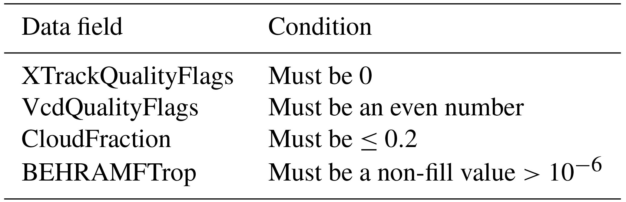
We compare against Pandora ground-based column measurements taken during the four DISCOVER-AQ campaigns. For each OMI overpass, pixels are matched with Pandora sites that lie within the pixel boundaries defined by the FoV75 corners in the OMPIXCOR product (Kurosu and Celarier, 2010). Only pixels meeting the criteria in Table 1 are used. If multiple valid pixels from the same overpass encompass the Pandora site, their VCDs are averaged. As in Goldberg et al. (2017), the stratospheric VCD from the NASA standard product is added to the tropospheric VCD to obtain a total column since the Pandora columns do not separate stratospheric and tropospheric contributions.
Table 1Criteria that OMI pixels must meet to be used in any comparison.
Pandora observations are matched in time to the OMI observations using the exact time of observation for each pixel given in the OMI data files. As in Goldberg et al. (2017), Pandora observations ±1 h from the OMI observation are averaged.
2.4 In situ aircraft profiles
The other common method of evaluating satellite VCDs is to use in situ measurements of NO2 by an instrumented aircraft that flies a vertical profile to calculate a VCD by integrating the NO2 concentrations vertically. Ideally, the aircraft should fly a spiral path that provides a complete vertical sampling of the troposphere over a ground footprint similar in scale to the satellite pixel; the DISCOVER-AQ campaigns held in Maryland, California, Texas, and Colorado between 2011 and 2014 were designed to provide this sampling over the lower troposphere. In other cases, the VCD calculated from integrating the aircraft profiles is often matched to satellite pixels in which the BL is sampled (Bucsela et al., 2008; Hains et al., 2010), on the assumption that UT sampling from adjacent pixels is sufficient.
We calculate tropospheric VCDs from in situ NO2 profiles measured from aircraft. We use six campaigns: the four DISCOVER-AQ campaigns (https://www-air.larc.nasa.gov/missions/discover-aq/discover-aq.html, last access: 3 January 2019) in Maryland (2011), California (2013), Texas (2013), and Colorado (2014); the Southeast Nexus campaign (SENEX Science Team, 2013); and the Studies of Emissions and Atmospheric Composition, Clouds, and Climate Coupling by Regional Surveys (Toon et al., 2016). For the DISCOVER-AQ and SEAC4RS campaigns, we use 1 s NO2 data from the thermal dissociation–laser-induced fluorescence (TD-LIF) instrument (Day et al., 2002; Nault et al., 2015; Thornton et al., 2000; Wooldridge et al., 2010). For the SENEX campaign, we use 1 s data from the chemiluminescence instrument (Ryerson et al., 1999).
We draw on methodology from several papers (Bucsela et al., 2008; Hains et al., 2010; Lamsal et al., 2014) for our approach. Similar to Hains et al. (2010), only profiles with a minimum radar altitude <500 m and at least 20 measurements below 3 km above ground level (a.g.l.) are used. In the DISCOVER-AQ campaigns, individual profiles are demarcated in the data by a profile number. In the SENEX and SEAC4RS data, profiles were identified manually as periods when the aircraft was consistently ascending or descending. The profile measurements are binned to the same pressure levels used in the BEHR algorithm and the final profile uses the median of each bin.
Profiles are spatially matched to OMI pixels if any of the 1 s measurements in the bottom 3 km a.g.l. lie within the FoV75 pixel boundaries. As with Pandora data, OMI pixels must meet the criteria in Table 1 to be included; all VCDs from valid pixels intersecting the profile are averaged to yield a single VCD to compare against the profile. Only profiles with a mean observation time of all points in the bottom 3 km a.g.l. within 1.5 h of the mean OMI observation time for the orbit are used.
To calculate a VCD from the in situ measurements, the aircraft profiles are integrated from the average surface pressure to the average tropopause pressure of the matched pixels. The surface and tropopause pressure are used from the product being evaluated, i.e., aircraft profiles are integrated between BEHR surface and tropopause pressure for comparison with BEHR VCDs and NASA surface and tropopause pressures for comparison with NASA VCDs. For BEHR v2.1C comparisons, 200 hPa is used as the fixed tropopause pressure. Aircraft profiles that do not span the necessary vertical extent are extended similarly to in Lamsal et al. (2014). The aircraft profile is extended to the surface by using the ratio of modeled concentrations at each of the missing levels to the lowest level with aircraft data to scale the bottom bin with aircraft data. Missing profile levels above the top of the aircraft profile are replaced with model data. We use modeled NO2 profiles from the “updated +33 %” GEOS-Chem simulation described in Nault et al. (2017) (v9.02 of the GEOS-Chem global chemical transport model (Bey et al., 2001) at resolution, with updated HNO3, HO2NO2, and N2O5 chemistry and lightning emission rates). The NO2 profiles are monthly averages of model output from 2012 sampled between 12:00 and 14:00 local standard time. We avoid using the a priori WRF-Chem profiles for this so that the aircraft VCDs are independent of the retrieved VCDs.
We also used the extrapolation method from Hains et al. (2010), in which the medians of the top 10 and bottom 10 points are extrapolated to the tropopause and surface pressures, respectively. The median of the top 10 points must be <100 pptv. As in Hains et al. (2010), a detection limit of 3 pptv is assumed, and if the median to be extrapolated is less than 3 pptv, it is set to one-half of the detection limit, 1.5 pptv.
In addition, we directly compare the a priori profiles to the in situ aircraft profiles. This is performed as in Laughner and Cohen (2017); for each 1 s data point in the aircraft data, the nearest WRF-Chem output time is selected, and the model grid cell containing the aircraft location is sampled. This effectively samples the model output as if the aircraft were flying through the model world.
We use a similar set of aircraft campaigns here as for the VCD evaluation (Sect. 2.4); the only difference being that we use the Deep Convective Clouds and Chemistry (DC3) (Barth et al., 2015) instead of SENEX. The DC3 campaign focused on outflow from convective systems (i.e., thunderstorms) and so is used to evaluate the lightning NOx parameterization. The DC3 campaign had better UT sampling but far fewer profiles than SENEX. The DISCOVER-AQ campaigns focused on satellite validation, flying repeated spirals over six to eight sites during each campaign; however, for the average comparison, we use all data, not just those taken during the spirals.
3.1 Comparison with in situ aircraft profiles
Figure 1 shows campaign-averaged profiles matched with WRF profiles from the four DISCOVER-AQ campaigns, the DC3 campaign, and the SEAC4RS campaign. We compare the monthly average NO2 profiles from BEHR v2.1C and v3.0B for all campaigns, as well as the daily v3.0B profiles. The plots shown only use data between 12:00 and 15:00 local standard time since the v3.0 monthly average profiles are calculated as a weighted average that only includes contributions from ±1 h from OMI overpass; this way all profiles get a fair comparison to the observations.
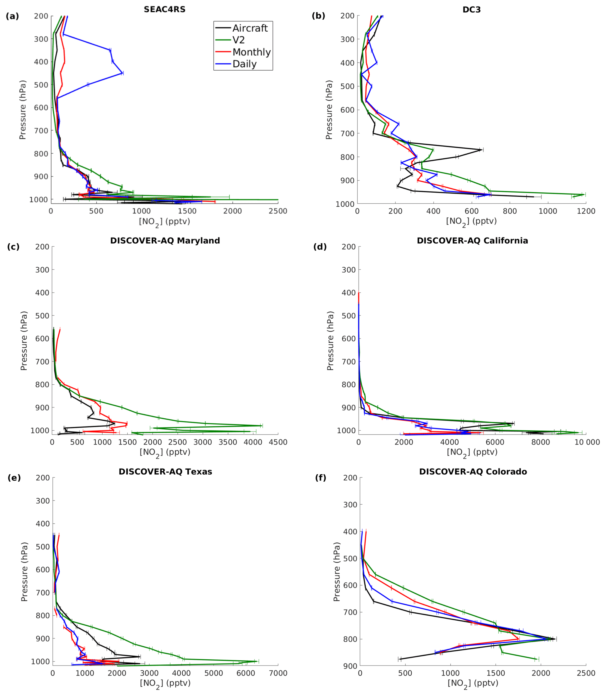
Figure 1Comparison of average WRF-Chem and aircraft NO2 profiles from the (a) SEAC4RS, (b) DC3, and DISCOVER-AQ campaigns, the latter in (c) Maryland, (d) California, (e) Texas, and (f) Colorado. Aircraft profiles are shown in black, BEHR v2.1 profiles in green, BEHR v3.0 monthly profiles in red, and (where available) BEHR v3.0 daily profiles in blue. The WRF and aircraft data are matched as described in Sect. 2.4 and binned by pressure. Uncertainties are 1 standard deviation of all profiles averaged. Note that for SEAC4RS the v2 profile reaches a maximum of ∼8000 pptv, off the plot axes.
In general, the v3.0 profiles show better agreement with observed profiles than the v2.1 profiles, except during the California DISCOVER-AQ campaign. The most dramatic example is the Maryland DISCOVER-AQ campaign, in which the factor of ∼2 reduction in NO2 concentration (likely due to updating emissions from 2005 to 2012, Fig. S10) brings the modeled profiles into substantially better agreement with the observed profiles. In the California DISCOVER-AQ campaign, the v2.1 profiles managed to capture an elevated layer of NO2 that the v3.0 profiles did not; though we note that transport in California's Central Valley is notorious difficult to model (Hu et al., 2010). In Texas, the v3.0 profiles and v2.1 profiles lie on opposite sides of the observed profiles, possibly suggesting that emissions in Houston did not decrease as much in fact as in the NEI inventory driving the v3.0 WRF simulations. In Colorado, both the v3.0 and v2.1 profiles match observations reasonably well. The daily profiles do a better job capturing the decrease in NO2 between 750 and 600 hPa than the v3.0 monthly or v2.1 profiles; this may be due to day-to-day variability in recirculation from the upslope–downslope winds (Sullivan et al., 2016).
Table 2Mean absolute bias between each of the types of simulated NO2 profiles and the aircraft profiles shown in Fig. 1. Values are given for the boundary layer (BL) and free troposphere (FT), with the divide at 775 hPa (∼2 km). All values are in parts per trillion by volume (pptv).

We evaluate the agreement quantitatively by calculating the mean absolute bias between the average WRF and aircraft profiles (Table 2). We divide the profiles into BL and FT, as different processes (e.g., anthropogenic vs. lightning emissions) govern them. As the SEAC4RS campaign has an obvious error in the FT (which will be discussed below), we calculate these values with and without the SEAC4RS campaign. In the BL, the version 3 profiles have one-half to two-thirds the bias of the version 2 profiles (depending on whether SEAC4RS is excluded). In the FT, there is little difference in the mean bias among profile types, unless SEAC4RS is included, in which case the daily profiles have a 33 % greater bias.
We include the SEAC4RS and DC3 campaigns to check the simulation of lightning NOx in the profiles. The daily profiles show agreement with the DC3 observations similar to that in Laughner and Cohen (2017). Restricting the DC3 data to 12:00–15:00 local standard time as we have done here reduces the strength of the lightning signal since the strongest lightning occurs after OMI overpass (Lay et al., 2007; Williams et al., 2000). Compared to Laughner and Cohen (2017), the discrepancy between modeled and observed profiles decreased around 500 hPa, increased around 400 hPa, and is similarly small around 200 hPa. Surprisingly, the difference between the v2.1 and v3.0 profile around 200 hPa is not as significant as the difference between the lightning and no-lightning cases in Laughner and Cohen (2017). This is unexpected as the v2.1 profiles did not include lightning NOx emission. It is possible that convection of greater surface NOx concentrations is driving the v2.1 UT concentration.
The SEAC4RS campaign covers the southeast US, which has very active lightning (Hudman et al., 2007; Travis et al., 2016). The daily profiles demonstrate a substantial overestimate in UT NO2 (between 600 and 200 hPa). This is centered in the southeast US; model–measurement discrepancies between 600 and 200 hPa in the rest of the country are <500 pptv (not shown). As discussed in Laughner et al. (2018f), the southeast US exhibits greater NO2 VCDs (and therefore smaller AMFs) when using daily profiles; that is opposite to the profiles seen here, as greater NO2 at higher altitudes results in larger AMFs. Laughner et al. (2018f) showed that the 3-month average daily shape factor over the southeast US had less contribution from UT NO2 than the monthly profiles; this indicates that on average pixels in the southeast US are not influenced by lightning, but that the SEAC4RS sampling tended to select for convective outflow. However, this does indicate that the simulation of the UT in the southeast US is biased high.

Figure 2Comparison between observed and simulated flash density from 13 May to 23 June 2012. Panels (a) and (b) show the mean flash density averaged over the study period from ENTLN and WRF-Chem, respectively. Both are gridded at 12 km grid spacing. Panels (c) and (d) show the correlation between total flash density per day between WRF and ENTLN in (c) the southeast US (denoted by the red box in a and b) and (d) elsewhere in the contiguous US.
To investigate the cause of this bias, we compare the WRF lightning flash density to that measured by the Earth Networks Total Lightning Network (ENTLN). ENTLN is a ground-based lightning observation network with more than 900 sensors deployed in the contiguous US. The sensors record lightning-produced strokes as well as accurate time and location. Strokes are then clustered into a flash if they are within 700 ms and 10 km of each other. The detection coefficient is larger than 70 % across the southern contiguous US (Rudlosky, 2015).
For the comparison, the WRF-Chem simulation is that described in Sect. 2.2. ENTLN and WRF-Chem are sampled from 13 May to 23 June 2012 over the middle and east US domain, where active lightning events are detected. Both observed and simulated lightning flashes are converted to flash density by dividing flash counts by corresponding grid areas and time range.
Figure 2a and b show the spatial distribution of flash density in number per square kilometer per day observed by ENTLN and simulated by WRF-Chem. The largest biases are located over the southeast US (outlined by red on the map). In this region, WRF-Chem substantially overestimates flash density in general and a detection coefficient of 70 % for ENTLN cannot account for the discrepancy. The simulated flash density is the highest primarily along the coast, which is not detected by ENTLN.
The scatter plot of daily flash density over the southeast US from two datasets in Fig. 2c demonstrates that the WRF-Chem consistently overestimates flashes in the southeast US over the study period. However, outside of the southeast US, the agreement improves. The simulation captures the spatial pattern over the regional scale (Fig. 2a and b) and the simulated flash densities are consistent with the observed flash densities and the correlation improves as well (Fig. 2d).
Currently, the cause of the discrepancies between the flash density from WRF-Chem simulation and ENTLN observation is unknown. However, it is clear that the flash density, rather than the per-flash production rate of NO, is the cause of the disagreement in the UT between the daily profiles and SEAC4RS data. Further research is required to optimize the lightning parameterizations and improve flash density simulations in the southeast US for our model simulation.
3.2 Evaluation of variability in daily profiles
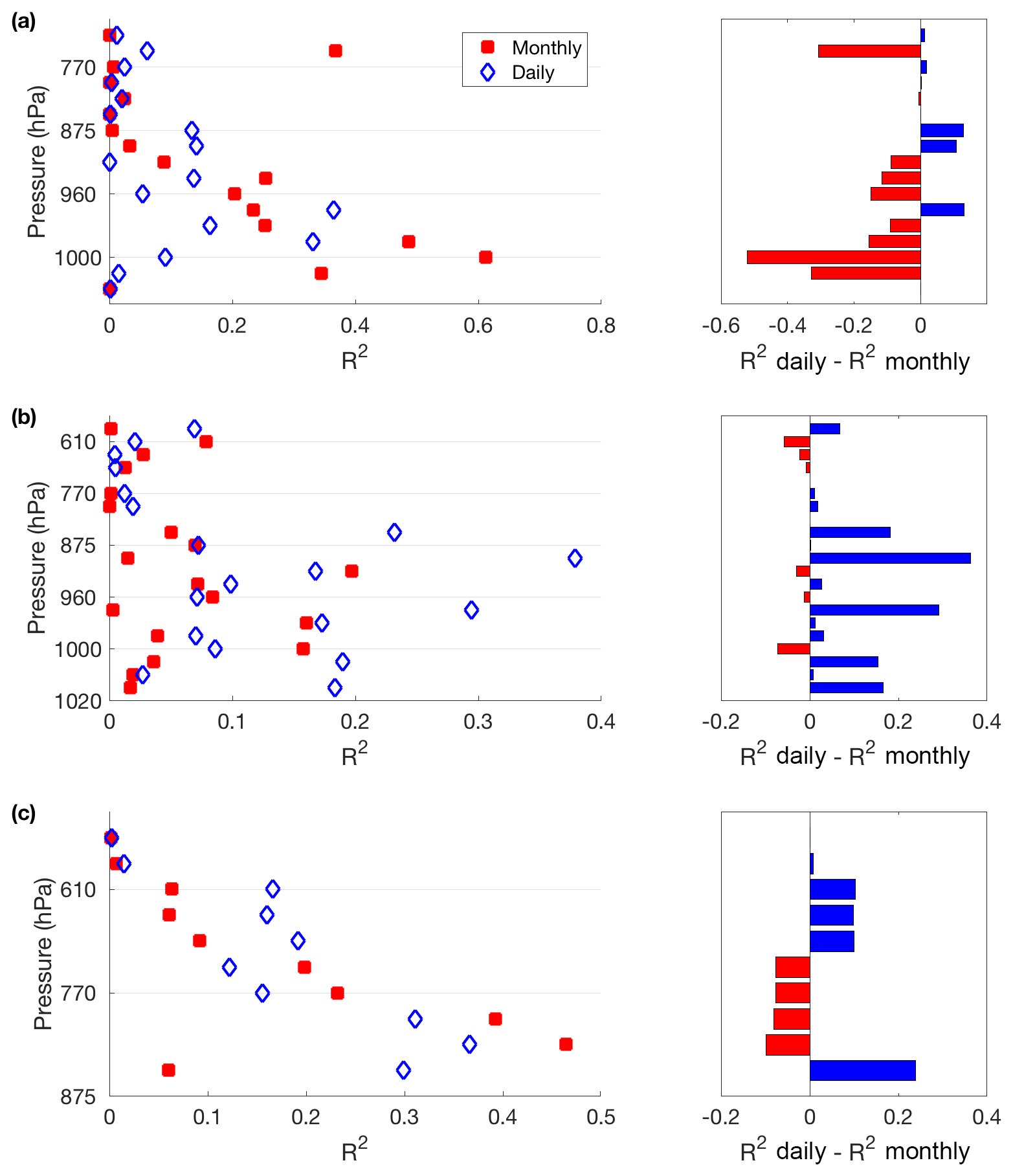
Figure 3R2 values for correlation between aircraft data and spatiotemporally matched WRF-Chem data for the (a) DISCOVER-CA, (b) DISCOVER-TX, and (c) DISCOVER-CO campaigns, binned by pressure. Left column shows absolute R2 values for each bin. Right column shows the difference in R2 values using monthly average and daily profiles for each bin.
As demonstrated in Laughner et al. (2016), simulating the day-to-day variability in the a priori NO2 profiles can have a significant impact on the retrieved NO2 VCDs due primarily to the day-to-day variation in wind speed and direction driving outflow from emissions sources, e.g., cities and power plants. To examine how well WRF-Chem captures the day-to-day variability in NO2 profiles, we compare aircraft data from three DISCOVER-AQ campaigns and the matched WRF-Chem data (Sect. 2.4). For each profile in the DISCOVER data, we binned the NO2 concentrations by pressure and calculated the correlation between WRF-Chem and aircraft NO2 concentrations (one data point per profile per pressure bin). The results are shown in Fig. 3.
In California (Fig. 3a), the monthly average profiles correlate better with the aircraft data. However, as mentioned before, the Californian Central Valley is known to be difficult to model accurately (Hu et al., 2010). In Colorado (Fig. 3c), the daily profiles do a slightly better job overall, simulating the variability at the surface and in an elevated layer more accurately than the monthly average profiles. The difference in Texas is quite dramatic (Fig. 3b), with the daily modeled profiles performing substantially better. This suggests that daily profiles are able to capture variability caused by small, concentrated urban plumes much more effectively than monthly average profiles.
As a second check, we also compare WRF-Chem tropospheric VCDs to OMI SCDs to evaluate the general accuracy of wind direction and speed in the daily model profiles. The OMI SCDs do not depend on modeled vertical profiles and so constitute an independent check on the plume direction. In order to have strong isolated NOx sources, we use Atlanta, Chicago, Las Vegas, Los Angeles, New York, and the Four Corners power plant for this study. For each of these sites, five days from 2007 are randomly chosen. If insufficient OMI SCDs are available for any day (>10 % of OMI pixels are cloud covered or in the row anomaly), another day is randomly chosen.
For each day, the agreement between the relative spatial distribution of WRF-Chem VCDs and OMI SCDs is manually evaluated, focusing on whether the model plume is advected in the same direction as the OMI SCDs indicate. Each day's agreement is evaluated qualitatively as good or bad. This, whether the WRF-Chem daily VCDs are significantly different from the monthly average WRF-Chem VCDs, and the confidence in the comparison are recorded for each comparison. Because of the number of factors that affect the absolute magnitude of SCDs, we look for qualitative, rather than statistically quantitative, agreement between the modeled VCDs and OMI SCDs. This is relevant since Laughner et al. (2016) noted that it is primarily the plume shape that drives the day-to-day variability in AMFs; therefore a direct qualitative evaluation of the plume shape is desirable.
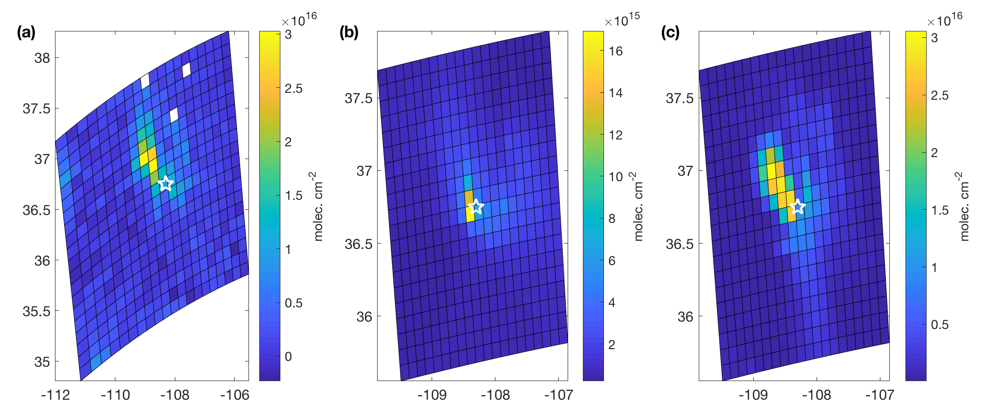
Figure 4A comparison of OMI SCDs (a) and WRF monthly average (b) and daily (c) VCDs. The star marks the location of the Four Corners power plant. Data are from 4 March 2007.
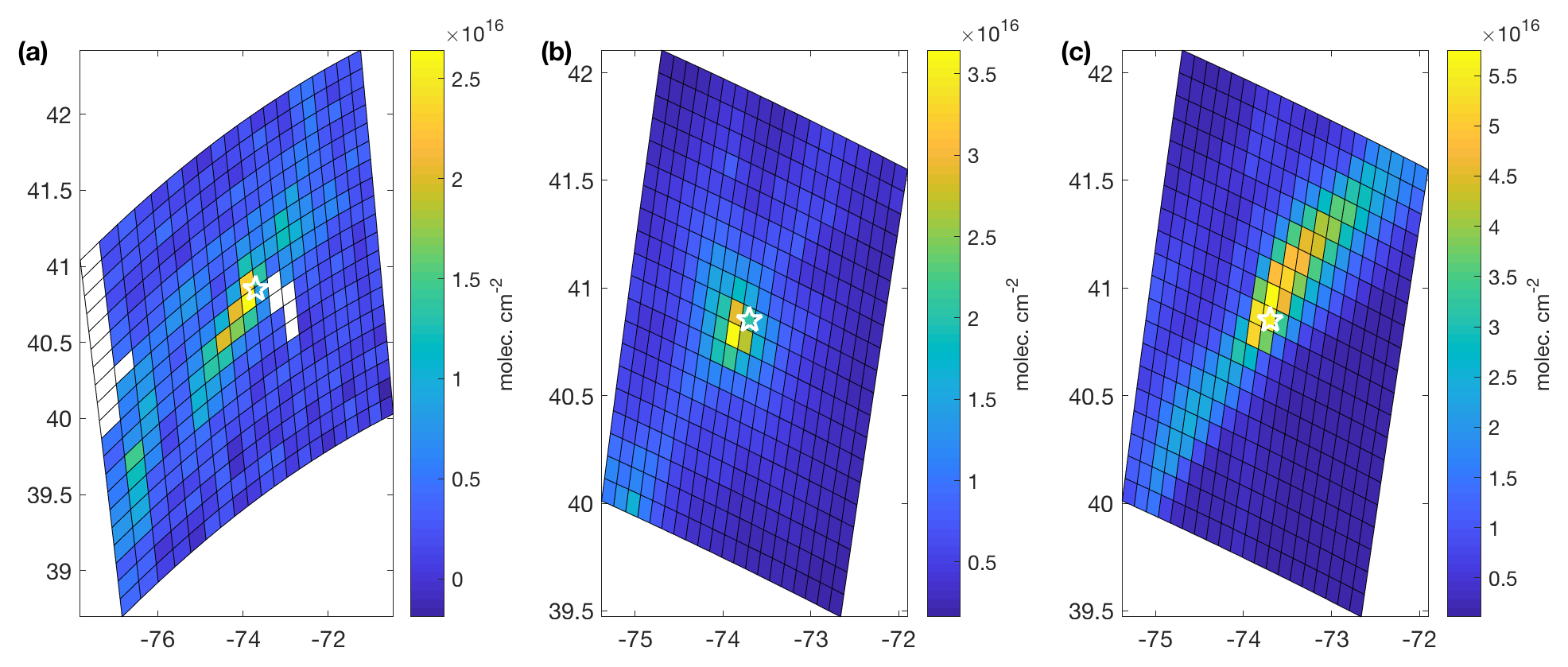
Figure 5A comparison of OMI SCDs (a) and WRF monthly average (b) and daily (c) VCDs. The star marks the location of New York, NY, USA. Data are from 29 September 2007.
Figures 4 and 5 show two example comparisons, one good (Fig. 4) and one poor (Fig. 5). By studying randomly chosen days for six large NOx sources, we find that about 67 %–73 % of days with sufficient data to be evaluated show good agreement between the OMI SCDs and WRF-Chem daily VCDs. (The range is due to different levels of confidence filtering.) This indicates that the WRF-Chem-simulated NO2 profiles are adequately capturing the day-to-day variability due to wind speed and direction. While we recognize that this conclusion is highly qualitative, the specific character of agreement that is important for these profiles (overall plume size and direction, rather than exact agreement between modeled and real concentrations or column densities) is rather difficult to evaluate quantitatively. We recognize that developing such methods is necessary and offer several possible approaches in Sect. 5.
Both comparisons (vs. OMI SCDs and aircraft measurements) show that daily WRF-Chem profiles do, on average, a better job than monthly average profiles capturing the day-to-day variation in profile shape. Therefore, the core improvement in BEHR v3.0, the transition to daily high-resolution a priori profiles, is fundamentally sound. Daily profiles are especially important for applications that focus on upwind–downwind differences in NO2 columns around a NOx source (Laughner et al., 2016) and, as we will see in Sect. 4, generally improve the retrieval in dense urban areas.
For the DISCOVER campaigns, we compare BEHR against aircraft-derived and Pandora VCDs together, calculating a single regression line for the combined dataset. These two measurements have unique strengths and weaknesses for comparison against satellite VCDs: Pandora spectrometers give precise column measurements and can be deployed for long time periods but have very small footprints (leading to possible representativeness errors) and provide total, not tropospheric, columns. Aircraft profiles have a footprint more similar to an OMI pixel size but introduce uncertainty due to missing parts of the profile (near the surface and in the UT in the DISCOVER campaigns) and cannot be deployed for long-term routine observations.
In order to take advantage of each method's strengths, we use two comparisons; in one, only Pandora data that have a coincident aircraft profile are included (“matched”), and in the other, all cloud-free Pandora data are used (“all”). We do so because, when including all Pandora data, the number of Pandora comparisons available will overwhelm the number of available aircraft profiles in the regression. Therefore the regressions using all Pandora data are representative of longer time periods but weighted strongly towards the Pandora data, and the regressions using only the coincident data represent shorter time periods but give more weight to the aircraft data. As stated in Sect. 2.3, we average all data within 1 h of OMI overpass (i.e., 13:30 local time ±1 h) to be consistent with Goldberg et al. (2017). A shorter averaging window (±0.5 h) was tested; the maximum effect on the slope was ∼8 % with most of the matched data slopes showing differences of ≤5 % and the all data slopes changing by ≤3.5 % in all but one case.
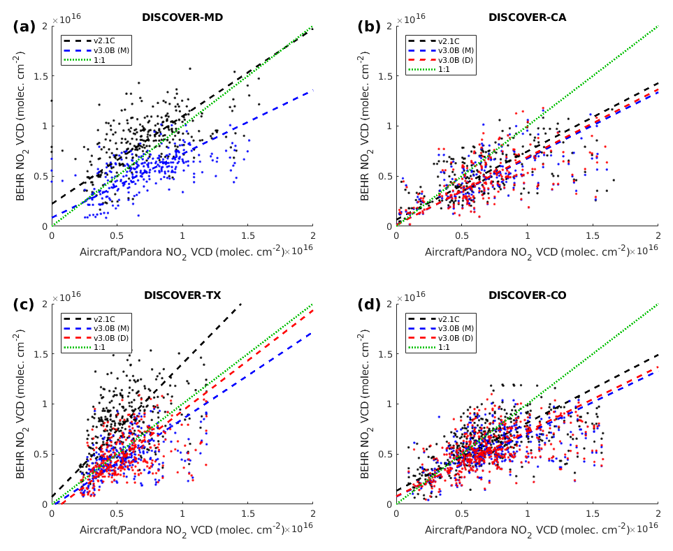
Figure 6Scatter plots of the BEHR v2.1C, v3.0B (M), and (where available) v3.0B (D) VCDs against coincident aircraft and Pandora VCDs. All Pandora VCDs are used for these plots. Each panel is one campaign: the (a) Maryland, (b) California, (c) Texas, and (d) Colorado DISCOVER-AQ campaigns. For slopes, see Table 3; for intercepts and R2 values, see Table S3.
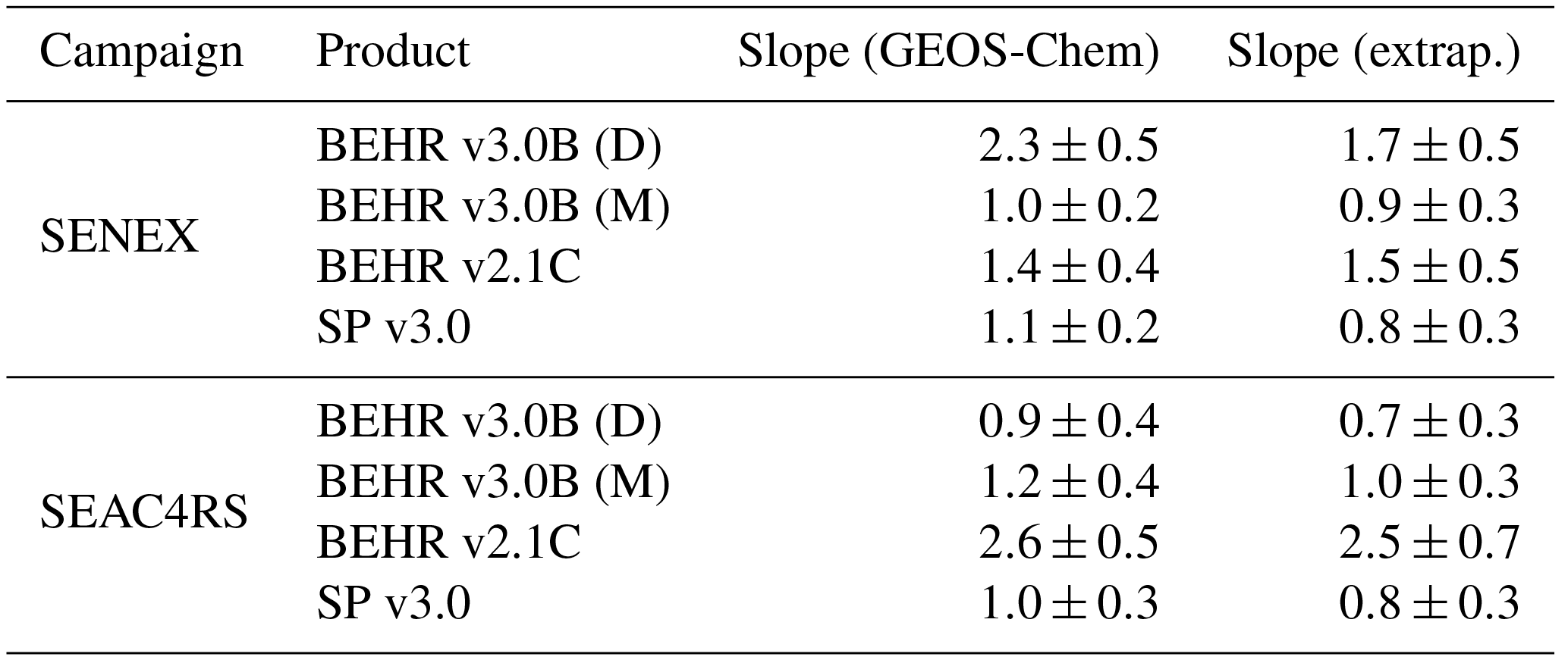
Slopes and their 1σ uncertainties for combined aircraft and Pandora VCDs are shown in Table 3. To evaluate the southeast US, we use the SENEX and SEAC4RS campaigns, which only have aircraft data. These results are shown in Table 4. More details (slope, intercepts, R2 values) can be found in Tables S1, S2, and S3. Figure 6 shows scatter plots of the BEHR vs. aircraft and all Pandora data for the four DISCOVER-AQ campaigns. Scatter plots showing aircraft and Pandora data separately are available in Sect. S1 of the Supplement.
For the DISCOVER-CO aircraft comparison, negative VCDs were removed. Negative VCDs occur when the estimated stratospheric NO2 column is greater than the total NO2 column; thus . They cannot be introduced by the AMF correction of the tropospheric SCD to VCD as the AMF is a multiplicative factor and always >0. Since all versions of BEHR use the same stratospheric NO2 column as their respective NASA SP products, an error in stratospheric subtraction will be present in all products, and it cannot be corrected in the BEHR retrieval. Aircraft VCDs, by their nature, cannot be negative, so for these comparisons we remove the negative VCDs so as to avoid increasing the regression slopes by trying to fit these erroneous points. (However, we do note that this is a special case in which individual pixels or small groups of pixels are being compared against other VCDs. Most applications of BEHR data should retain the negative VCDs to avoid transforming the essentially Gaussian random stratospheric error into a systematic error by removing part of the bell curve.) Since the stratospheric VCDs are added back to the BEHR or NASA SP tropospheric VCDs for comparison with the Pandora VCDs, negative VCDs are not an issue with Pandora comparisons.
In the following sections, we will evaluate the new BEHR v3.0 VCDs from three perspectives: performance compared to the current NASA SP, performance compared to the previous version of BEHR, and performance using daily a priori profiles compared to using monthly a priori profiles. Throughout, BEHR v3.0 (M) refers to BEHR using monthly NO2 profiles; likewise, BEHR v3.0 (D) refers to the product using daily NO2 profiles. We will focus on the regression slopes here; intercepts and R2 values are given in Table S3 in the Supplement; however we note that there is not a clear pattern of any one product having a consistently better R2 value than the others.
Table 3Slopes and 1σ uncertainties of BEHR vs. combined aircraft (extended with GEOS-Chem profiles) and Pandora VCDs. Matched slopes use only Pandora data approximately coincident with aircraft profiles to obtain similar sampling; all uses all valid Pandora data. Outliers and negative VCDs are removed before computing slopes.
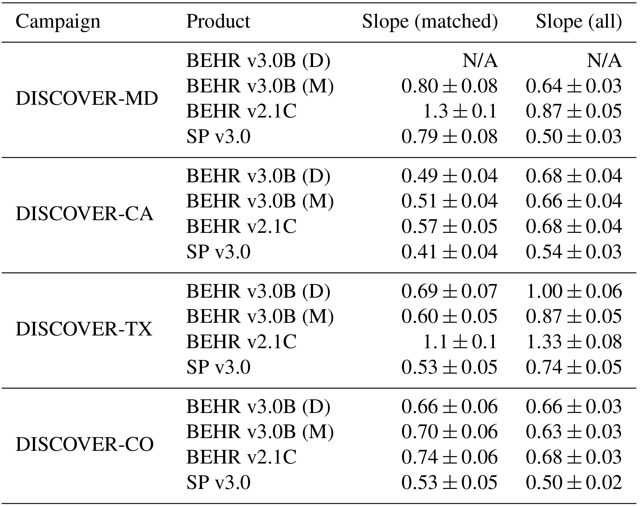
Table 4Slopes and 1σ uncertainties for reduced major axis (RMA) regression of satellite VCDs against in situ calculated VCDs. Both methods of extending the profiles (using GEOS-Chem modeled profiles or extrapolating the top and bottom 10 points) are included. Outliers are removed before calculating these parameters.
4.1 Comparison vs. SP v3.0
For all the DISCOVER campaigns, BEHR v3.0 shows better agreement with both aircraft and Pandora measurements than the NASA SP v3.0 (slopes closer to 1). This is expected since these campaigns generally centered on one or more cities, and a key feature of the BEHR retrieval is the ∼12 km a priori profiles (∼10× higher resolution than the NASA SP v3.0 profiles), which better capture the urban profile shape.
In the SENEX and SEAC4RS campaigns, BEHR's performance is more mixed. These campaigns include the southeast US, where we found that the WRF-Chem simulation that generated the a priori profiles overestimated the lightning flash density (Sect. 3.1). In SEAC4RS, whether BEHR v3.0 (M) performs better or worse than the NASA SP v3.0 depends on the method used to extend the profile (Sect. 2.4). This indicates that uncertainty in the measurement is greater than the difference between these two products. BEHR v3.0 (D) performs poorly in the SENEX campaign; this will be explored in Sect. 4.3. Overall, BEHR v3.0 (M) is not significantly affected by the overestimated lightning flash density in the southeast US, as the monthly average profiles smooth out the overlarge UT lightning NO2 signal.
4.2 Comparison vs. BEHR v2.1
Using aircraft data plus just Pandora data coincident with aircraft spirals, v2.1 performs better in all DISCOVER campaigns except MD. However, using aircraft data plus all Pandora data, v3.0 (D) performs better than or similar to v2.1 in all DISCOVER campaigns in which daily profiles are available. The Pandora spectrometers provide more observations than the aircraft profiles, and, due to their small footprint, are more sensitive to narrow, highly concentrated NO2 plumes. The v2.1 profiles used 2005 emissions; as seen in Fig. 1, this led to too much NO2 being placed at the surface, which will increase the retrieved VCD. This suggests that the better performance of v2.1 in some cases is due to cancellation of errors; overestimated surface NO2 is canceling out the lack of temporal variation in the profiles. That is, the higher average surface concentration in the v2.1 profiles may be similar to the in-plume concentrations resolved by the daily v3.0 profiles.
In v3.0, when daily profiles are available, the agreement is similar to or better than v2.1 if aircraft and all Pandora data are used. Therefore, daily profiles are able to capture at least some enhancements in surface NO2 where and when they occur, without overestimating the average profile. This is not evident using aircraft and just the coincident Pandora data because of the smaller number of comparisons. As the comparison expands (using all Pandora data), the improvement becomes evident. The better performance of daily profiles suggests that even though Laughner et al. (2016) did not see large effects in a multi-month average using daily instead of monthly profiles, daily profiles will provide a more accurate representation of urban VCDs over longer averaging periods.
BEHR v3.0 performs better in the SENEX and SEAC4RS comparisons than v2.1 (excluding 3.0 (D) in SENEX). The v2.1 profiles did not include lightning emissions, as it was a limitation of WRF-Chem at that time (Laughner et al., 2018f). This indicates that, even though the contribution of lightning to the southeast US profiles is too large, the inclusion of lightning NO2 in the profiles did improve the representation of the southeast US. Laughner et al. (2018f) also showed that implementing a variable tropopause pressure decreased VCDs in the southeast US during summer; this also would help reduce the high bias compared to SENEX and SEAC4RS seen in BEHR v2.1.
4.3 Comparison of BEHR v3.0 (M) vs. BEHR v3.0 (D) in the SE US
In the SENEX campaign, v3.0 (D) performs significantly worse than v3.0 (M). From Fig. 1 we know that the daily a priori profiles overestimate the UT NO2, and from Fig. 2 we know that this is due to a significant overestimate of the flash density in our WRF simulation. The comparison in Table 4 would seem to indicate that this overestimate has a severe impact on the retrieved VCDs, but we must also consider the uncertainty in the SENEX-derived VCDs.

Figure 7(a, b) The profiles used to calculate the aircraft VCDs extended using WRF-Chem or GEOS-Chem profiles; the solid line is the median of all profiles, and the shading represents the 10th and 90th percentiles for each binned level. Circles indicate levels that were derived from the models in at least 50 % of the profiles. (c, d) Comparison of BEHR v3.0 (D) VCDs vs. aircraft-derived VCDs using GEOS-Chem and WRF-Chem profiles to extend the profile to the surface and tropopause. The black lines connect corresponding comparisons between the two methods and the red dashed line represents the 1:1 agreement. (e, f) Difference between aircraft VCDs extended with WRF-Chem and GEOS-Chem profiles. Panels (a, c, e) are for the SENEX campaign, and (b, d, f) are for SEAC4RS.
Figure 7a shows the ensemble of profiles from SENEX used to calculate VCDs. The circles mark levels that had to be calculated using model data for >50 % of the profiles. In SENEX, that is all levels at about ∼700 hPa, which means that the SENEX aircraft data provide very little constraint on the UT. The lightning contribution to the SENEX columns must come from the GEOS-Chem monthly averages or extrapolation from a lower altitude, which means the spatial and temporal variation is lost.
Figure 7c shows the effect of using the WRF-Chem a priori profiles instead of the GEOS-Chem profiles to extend the SENEX profiles. The WRF-Chem profiles do include spatial and temporal variation in the UT, but using them reinforces the AMF errors, moving all points away from the 1:1 line. Without either in situ measurements of the UT in the southeast US or Pandora total column observations we cannot separate the errors in AMF caused by the overestimated UT NO2 in the a priori profiles from the error caused by the lack of spatiotemporal variation in the extended aircraft profiles. For example, the error in the cluster of points below the 1:1 line in Fig. 7c could be corrected if either the UT NO2 in the a priori profile was reduced, decreasing the AMFs and so increasing the BEHR VCDs, or if the aircraft profile had less NO2, thus moving the points left onto the 1:1 line. (In this case, there would still be a discrepancy between the BEHR VCD and the VCD derived from combining aircraft and WRF-Chem profiles, suggesting that the WRF-Chem UT NO2 is still too great.)
Other campaigns do have better sampling of the UT, e.g., SEAC4RS (Fig. 7b, d, f), but do not have as many profiles in the southeast US (Fig. 7e, f). Therefore, we must currently assign an uncertainty of ±100 % to VCDs retrieved with daily profiles in the southeast US (east of 95∘ W and south of 37.5∘ N). This is almost certainly overly conservative, as Laughner et al. (2018f) showed that the frequency distribution of UT NO2 in the southeast a priori profiles was skewed to lower values in the daily profiles, and a 3-month average using daily a priori profiles resulted in greater VCDs than using monthly a priori profiles, which would not be the case if the daily profiles always overestimated the UT. This suggests that days with little or no lightning in both the real world and WRF-Chem simulations are more numerous than days with a significant lightning contribution, and so a multi-month average using daily profiles would in fact accurately capture this. However, without long-term independent column measurements in the southeast, we cannot confirm this hypothesis. Future work will focus on improving the simulation of lightning in the southeast US. If successful, improved WRF-Chem profiles for the southeast can be implemented.
4.4 Comparison of BEHR v3.0 (M) vs. BEHR v3.0 (D) in urban areas
In the DISCOVER campaigns, BEHR v3.0 (D) using daily profiles has regression slopes similar to or closer to 1 than BEHR v3.0 (M) using monthly profiles except in the DISCOVER-CA aircraft comparisons. There is a clear improvement in DISCOVER-TX using daily profiles. This suggests that the daily profiles are capturing small concentrated plumes in the urban area (Fig. 3b), which is improving the retrieval overall in an urban area with many highly concentrated industrial NOx sources. Therefore, we argue that daily profiles improve the retrieval in many ways, not only for applications that select for upwind–downwind pixels as shown in Laughner et al. (2016), but also for multi-month averages in dense urban areas.
Using space-based SCDs to evaluate the spatial distribution of NO2 in a chemical transport model (CTM) is powerful (Sect. 3.2) because both the SCDs and CTM provide a spatially continuous field of NO2 columns. As we have shown here, this makes a qualitative evaluation straightforward and illustrative. However, a quantitative metric is more challenging to devise, as the direct correlation of model and satellite columns is less important than the more abstract agreement between the overall plume direction and extent. As we have shown here, daily high-resolution profiles provide important benefits to an NO2 retrieval; therefore, development of more quantitative methods to evaluate model performance in this manner should be a priority.
There are several possibilities. First, an algorithm that identifies the plume and computes the direction and length of its major axis could be used. This would allow a comparison of the direction and extent of the plumes more directly. Such an algorithm would not be trivial to develop; comparisons such as the one shown in Fig. 5a, c would likely be difficult for the algorithm to distinguish the plume direction accurately.
Second, this problem could be treated as an image recognition problem. A neural network could be trained on modeled VCDs and SCDs. A training set of good and bad days could be constructed from the WRF-Chem simulations used in BEHR v3.0 (D). Development of this approach is beyond the scope of this paper.
Third, dense sensor networks (Kim et al., 2018; Shusterman et al., 2016) may also be useful to evaluate daily profiles by permitting a simpler correlation test between modeled and observed surface concentrations than is possible between modeled VCDs and observed SCDs. Development of these networks is a topic of active research. This method may be necessary for future retrievals, especially over the US and European domains, where decreasing NOx emissions mean that the contrast between plumes and background in SCDs is much weaker now than in 2007.
We have evaluated version 3.0B of the BEHR OMI NO2 product against multiple datasets. We find that the WRF simulation used to generate the a priori NO2 profiles generally agrees well with the available aircraft data; however, the number of lightning flashes is significantly overestimated in the southeast US, leading to an overestimate of the UT NO2 in that region, although broadly consistent with ENTLN observations elsewhere. When compared against aircraft-derived and Pandora VCDs, BEHR v3.0B performs better than SP v3.0, with regionally varying low biases of 0 %–51 % compared to in situ and Pandora measurements. Using daily profiles yields better results than monthly profiles, except in the southeast US.
The lessons learned here are applicable to geostationary satellites scheduled to launch in the near future. Because the BEHR retrieval focuses on the continental US, it serves as a useful prototype for future NO2 retrievals from geostationary satellites such as GEMS (Bak et al., 2013; Choi and Ho, 2015), Sentinel-4 (Ingmann et al., 2012), and TEMPO (Chance et al., 2013), which will also be inherently restricted to regional areas. This offers the opportunity to use higher-resolution a priori data than global retrievals.
Here, the results from the SENEX and SEAC4RS campaign demonstrate that verifying the chemical transport model's reproduction of the day-to-day variability in lightning flashes is vital to obtain reliable results in such regions. With the sub-daily temporal resolution available to geostationary satellites, this will only become more important. Therefore, geostationary retrievals should evaluate the diurnal variation in lightning flashes in their a priori models using ground- and space-based lightning detectors (e.g., NLDN, ENTLN, or the GOES-R lightning mapper), and plans should be made to validate retrieved VCDs in multiple regions that have strong, but different, lightning influence. Such validations must include measurement of the UT NO2 profile and/or total column observations in order to reliably separate errors in the a priori profiles from errors in the observations used for evaluation.
Evaluating the day-to-day performance of the a priori profiles in future geostationary retrievals is crucial. Daily profiles have been shown to significantly affect retrieved NO2, especially in applications that systematically focus on NO2 VCDs downwind of a source (Laughner et al., 2016), and we have shown here that daily profiles also improve performance in urban areas. With the WRF-Chem model configuration used here, urban NO2 plumes are simulated with the correct spatial pattern ∼70 % of the time. Planned campaigns to evaluate geostationary satellite retrievals should be designed with an eye towards also evaluating the day-to-day accuracy of the a priori profiles.
The analysis code for this paper is available at https://github.com/behr-github/BEHR-v3-evaluation/ (Laughner, 2018). Supporting datasets generated or used by this code are hosted by UC Dash (Laughner et al., 2018e). The BEHR v3.0B product is hosted as four subproducts by UC Dash (Laughner et al., 2018a, b, c, d) as well as on http://behr.cchem.berkeley.edu/ (last access: 3 January 2019). The BEHR algorithm is available at https://github.com/CohenBerkeleyLab/BEHR-core/tree/master (Laughner and Zhu, 2018).
The supplement related to this article is available online at: https://doi.org/10.5194/amt-12-129-2019-supplement.
The authors declare that they have no conflict of interest.
JLL, QZ, and RCC articulated a plan for validating v3.0B of the BEHR algorithm. JLL and QZ executed that plan; JLL led the writing of the paper with input from QZ and RCC. RCC provided guidance and and acted as a mentor throughout the project and secured funding. All the authors reviewed the paper.
The authors gratefully acknowledge support from the NASA ESS Fellowship NNX14AK89H, NASA grant NNX15AE37G, and the TEMPO project grant SV3-83019.
We would like to acknowledge high-performance computing support from Cheyenne (https://doi.org/10.5065/D6RX99HX) provided by NCAR's Computational and Information Systems Laboratory, sponsored by the National Science Foundation. This research also used the Savio computational cluster resource provided by the Berkeley Research Computing program at the University of California, Berkeley (supported by the UC Berkeley Chancellor, Vice Chancellor for Research, and Chief Information Officer).
We acknowledge use of the WRF-Chem preprocessor tools MOZBC, fire_emiss, etc. provided by the Atmospheric Chemistry Observations and Modeling (ACOM) laboratory of NCAR.
Finally, we acknowledge the use of in situ NO2 measurements from the
UC Berkeley TD-LIF instrument and the NOAA chemiluminescence instrument, as
well as ground-based NO2 columns from multiple Pandora spectrometers
operated by various groups throughout the DISCOVER-AQ
campaigns.
Edited by: Jun Wang
Reviewed by: two anonymous referees
Bak, J., Kim, J. H., Liu, X., Chance, K., and Kim, J.: Evaluation of ozone profile and tropospheric ozone retrievals from GEMS and OMI spectra, Atmos. Meas. Tech., 6, 239–249, https://doi.org/10.5194/amt-6-239-2013, 2013. a
Barth, M. C., Cantrell, C. A., Brune, W. H., Rutledge, S. A., Crawford, J. H., Huntrieser, H., Carey, L. D., MacGorman, D., Weisman, M., Pickering, K. E., Bruning, E., Anderson, B., Apel, E., Biggerstaff, M., Campos, T., Campuzano-Jost, P., Cohen, R., Crounse, J., Day, D. A., Diskin, G., Flocke, F., Fried, A., Garland, C., Heikes, B., Honomichl, S., Hornbrook, R., Huey, L. G., Jimenez, J. L., Lang, T., Lichtenstern, M., Mikoviny, T., Nault, B., O'Sullivan, D., Pan, L. L., Peischl, J., Pollack, I., Richter, D., Riemer, D., Ryerson, T., Schlager, H., Clair, J. S., Walega, J., Weibring, P., Weinheimer, A., Wennberg, P., Wisthaler, A., Wooldridge, P. J., and Ziegler, C.: The Deep Convective Clouds and Chemistry (DC3) Field Campaign, B. Am. Meteorol. Soc., 96, 1281–1309, https://doi.org/10.1175/bams-d-13-00290.1, 2015. a
Beirle, S., Platt, U., Wenig, M., and Wagner, T.: NOx production by lightning estimated with GOME, Adv. Space Res., 34, 793–797, https://doi.org/10.1016/j.asr.2003.07.069, 2004. a
Beirle, S., Huntrieser, H., and Wagner, T.: Direct satellite observation of lightning-produced NOx, Atmos. Chem. Phys., 10, 10965–10986, https://doi.org/10.5194/acp-10-10965-2010, 2010. a
Beirle, S., Boersma, K., Platt, U., Lawrence, M., and Wagner, T.: Megacity Emissions and Lifetimes of Nitrogen Oxides Probed from Space, Science, 333, 1737–1739, 2011. a
Bertram, T. H., Heckel, A., Richter, A., Burrows, J. P., and Cohen, R. C.: Satellite measurements of daily variations in soil NOx emissions, Geophys. Res. Lett., 32, L24812, https://doi.org/10.1029/2005gl024640, 2005. a
Bey, I., Jacob, D. J., Yantosca, R. M., Logan, J. A., Field, B. D., Fiore, A. M., Li, Q., Liu, H. Y., Mickley, L. J., and Schultz., M. G.: Global modeling of tropospheric chemistry with assimilated meteorology, J. Geophys. Res., 106, 23073–23096, 2001. a
Boersma, F., Bucsela, E., Brinksma, E., and Gleason, J. F.: NO2 in: OMI Algorithm Theoretical Basis Document, Volume IV, OMI Trace Gas Algorithms, edited by: Chance, K., Tech. rep., Smithsonian Astrophysical Observatory, 2001. a
Boersma, K. F., Eskes, H. J., Veefkind, J. P., Brinksma, E. J., van der A, R. J., Sneep, M., van den Oord, G. H. J., Levelt, P. F., Stammes, P., Gleason, J. F., and Bucsela, E. J.: Near-real time retrieval of tropospheric NO2 from OMI, Atmos. Chem. Phys., 7, 2103–2118, https://doi.org/10.5194/acp-7-2103-2007, 2007. a
Bousserez, N.: Space-based retrieval of NO2 over biomass burning regions: quantifying and reducing uncertainties, Atmos. Meas. Tech., 7, 3431–3444, https://doi.org/10.5194/amt-7-3431-2014, 2014. a
Browne, E. C., Perring, A. E., Wooldridge, P. J., Apel, E., Hall, S. R., Huey, L. G., Mao, J., Spencer, K. M., Clair, J. M. St., Weinheimer, A. J., Wisthaler, A., and Cohen, R. C.: Global and regional effects of the photochemistry of CH3O2NO2: evidence from ARCTAS, Atmos. Chem. Phys., 11, 4209–4219, https://doi.org/10.5194/acp-11-4209-2011, 2011. a
Bucsela, E. J., Krotkov, N. A., Celarier, E. A., Lamsal, L. N., Swartz, W. H., Bhartia, P. K., Boersma, K. F., Veefkind, J. P., Gleason, J. F., and Pickering, K. E.: A new stratospheric and tropospheric NO2 retrieval algorithm for nadir-viewing satellite instruments: applications to OMI, Atmos. Meas. Tech., 6, 2607–2626, https://doi.org/10.5194/amt-6-2607-2013, 2013. a
Bucsela, E. J., Perring, A. E., Cohen, R. C., Boersma, K. F., Celarier, E. A., Gleason, J. F., Wenig, M. O., Bertram, T. H., Wooldridge, P. J., Dirksen, R., and Veefkind, J. P.: Comparison of tropospheric NO2 from in situ aircraft measurements with near-real-time and standard product data from OMI, J. Geophys. Res.-Atmos., 113, D16S31, https://doi.org/10.1029/2007JD008838, 2008. a, b, c
Bucsela, E. J., Pickering, K. E., Huntemann, T. L., Cohen, R. C., Perring, A., Gleason, J. F., Blakeslee, R. J., Albrecht, R. I., Holzworth, R., Cipriani, J. P., Vargas-Navarro, D., Mora-Segura, I., Pacheco-Hernández, A., and Laporte-Molina, S.: Lightning-generated NOx seen by the Ozone Monitoring Instrument during NASA's Tropical Composition, Cloud and Climate Coupling Experiment (TC4), J. Geophys. Res.-Atmos., 115, d00J10, https://doi.org/10.1029/2009JD013118, 2010. a
Burrows, J. P., Weber, M., Buchwitz, M., Rozanov, V., Ladstätter-Weißenmayer, A., Richter, A., DeBeek, R., Hoogen, R., Bramstedt, K., Eichmann, K.-U., and Eisinger, M.: The Global Ozone Monitoring Experiment (GOME): Mission Concept and First Scientific Results, J. Atmos. Sci., 56, 151–175, https://doi.org/10.1175/1520-0469(1999)056<0151:TGOMEG>2.0.CO;2, 1999. a
Castellanos, P. and Boersma, K. F.: Reductions in nitrogen oxides over Europe driven by environmental policy and economic recession, Sci. Rep., 2, 265, https://doi.org/10.1038/srep00265, 2012. a
Castellanos, P., Boersma, K. F., Torres, O., and de Haan, J. F.: OMI tropospheric NO2 air mass factors over South America: effects of biomass burning aerosols, Atmos. Meas. Tech., 8, 3831–3849, https://doi.org/10.5194/amt-8-3831-2015, 2015. a
Chance, K., Liu, X., Suleiman, R. M., Flittner, D. E., Al-Saadi, J., and Janz, S. J.: Tropospheric emissions: monitoring of pollution (TEMPO), Proc. SPIE, 8866, Earth Observing Systems XVIII, 88660D (23 September 2013), https://doi.org/10.1117/12.2024479, 2013. a
Choi, Y.-S. and Ho, C.-H.: Earth and environmental remote sensing community in South Korea: A review, Remote Sens. Appl., 2, 66–76, https://doi.org/10.1016/j.rsase.2015.11.003, 2015. a
Computational and Information Systems Laboratory: Cheyenne: HPE/SGI ICE XA System (NCAR Community Computing), Boulder, CO: National Center for Atmospheric Research, https://doi.org/10.5065/D6RX99HX, 2017.
Day, D. A., Wooldridge, P. J., Dillon, M. B., Thornton, J. A., and Cohen, R. C.: A thermal dissociation laser-induced fluorescence instrument for in situ detection of NO2, peroxy nitrates, alkyl nitrates, and HNO3, J. Geophys. Res.-Atmos., 107, 4046, https://doi.org/10.1029/2001JD000779, 2002. a
EPA: Air Pollutant Emissions Trends Data, available at: https://www.epa.gov/air-emissions-inventories/air-pollutant-emissions-trends-data, last access: 11 October 2016. a
Goldberg, D. L., Lamsal, L. N., Loughner, C. P., Swartz, W. H., Lu, Z., and Streets, D. G.: A high-resolution and observationally constrained OMI NO2 satellite retrieval, Atmos. Chem. Phys., 17, 11403–11421, https://doi.org/10.5194/acp-17-11403-2017, 2017. a, b, c, d, e
Grell, G. A., Peckham, S. E., Schmitz, R., McKeen, S. A., Frost, G., Skamarock, W. C., and Eder, B.: Fully coupled “online” chemistry within the {WRF} model, Atmos. Environ., 39, 6957–6975, https://doi.org/10.1016/j.atmosenv.2005.04.027, 2005. a
Guenther, A., Karl, T., Harley, P., Wiedinmyer, C., Palmer, P. I., and Geron, C.: Estimates of global terrestrial isoprene emissions using MEGAN (Model of Emissions of Gases and Aerosols from Nature), Atmos. Chem. Phys., 6, 3181–3210, https://doi.org/10.5194/acp-6-3181-2006, 2006. a
Hains, J. C., Boersma, K. F., Kroon, M., Dirksen, R. J., Cohen, R. C., Perring, A. E., Bucsela, E., Volten, H., Swart, D. P. J., Richter, A., Wittrock, F., Schoenhardt, A., Wagner, T., Ibrahim, O. W., van Roozendael, M., Pinardi, G., Gleason, J. F., Veefkind, J. P., and Levelt, P.: Testing and improving OMI DOMINO tropospheric NO2using observations from the DANDELIONS and INTEX-B validation campaigns, J. Geophys. Res., 115, D05301, https://doi.org/10.1029/2009jd012399, 2010. a, b, c, d, e, f, g
Herman, J., Cede, A., Spinei, E., Mount, G., Tzortziou, M., and Abuhassan, N.: NO2 column amounts from ground-based Pandora and MFDOAS spectrometers using the direct-sun DOAS technique: Intercomparisons and application to OMI validation, J. Geophys. Res.-Atmos., 114, D13307, https://doi.org/10.1029/2009jd011848, 2009. a, b
Hönninger, G., von Friedeburg, C., and Platt, U.: Multi axis differential optical absorption spectroscopy (MAX-DOAS), Atmos. Chem. Phys., 4, 231–254, https://doi.org/10.5194/acp-4-231-2004, 2004. a
Hu, J., Ying, Q., Chen, J., Mahmud, A., Zhao, Z., Chen, S.-H., and Kleeman, M. J.: Particulate air quality model predictions using prognostic vs. diagnostic meteorology in central California, Atmos. Environ., 44, 215–226, https://doi.org/10.1016/j.atmosenv.2009.10.011, 2010. a, b
Hudman, R. C., Jacob, D. J., Turquety, S., Leibensperger, E. M., Murray, L. T., Wu, S., Gilliland, A. B., Avery, M., Bertram, T. H., Brune, W., Cohen, R. C., Dibb, J. E., Flocke, F. M., Fried, A., Holloway, J., Neuman, J. A., Orville, R., Perring, A., Ren, X., Sachse, G. W., Singh, H. B., Swanson, A., and Wooldridge, P. J.: Surface and lightning sources of nitrogen oxides over the United States: Magnitudes, chemical evolution, and outflow, J. Geophys. Res., 112, D12S05, https://doi.org/10.1029/2006jd007912, 2007. a
Hudman, R. C., Russell, A. R., Valin, L. C., and Cohen, R. C.: Interannual variability in soil nitric oxide emissions over the United States as viewed from space, Atmos. Chem. Phys., 10, 9943–9952, https://doi.org/10.5194/acp-10-9943-2010, 2010. a
Hudman, R. C., Moore, N. E., Mebust, A. K., Martin, R. V., Russell, A. R., Valin, L. C., and Cohen, R. C.: Steps towards a mechanistic model of global soil nitric oxide emissions: implementation and space based-constraints, Atmos. Chem. Phys., 12, 7779–7795, https://doi.org/10.5194/acp-12-7779-2012, 2012. a
Huijnen, V., Flemming, J., Kaiser, J. W., Inness, A., Leitão, J., Heil, A., Eskes, H. J., Schultz, M. G., Benedetti, A., Hadji-Lazaro, J., Dufour, G., and Eremenko, M.: Hindcast experiments of tropospheric composition during the summer 2010 fires over western Russia, Atmos. Chem. Phys., 12, 4341–4364, https://doi.org/10.5194/acp-12-4341-2012, 2012. a
Ialongo, I., Herman, J., Krotkov, N., Lamsal, L., Boersma, K. F., Hovila, J., and Tamminen, J.: Comparison of OMI NO2 observations and their seasonal and weekly cycles with ground-based measurements in Helsinki, Atmos. Meas. Tech., 9, 5203–5212, https://doi.org/10.5194/amt-9-5203-2016, 2016 a
Ingmann, P., Veihelmann, B., Langen, J., Lamarre, D., Stark, H., and Courrèges-Lacoste, G. B.: Requirements for the {GMES} Atmosphere Service and ESA's implementation concept: Sentinels-4/-5 and -5p, Remote Sens. Environ., 120, 58–69, https://doi.org/10.1016/j.rse.2012.01.023, 2012. a
Kim, J., Shusterman, A. A., Lieschke, K. J., Newman, C., and Cohen, R. C.: The BErkeley Atmospheric CO2 Observation Network: field calibration and evaluation of low-cost air quality sensors, Atmos. Meas. Tech., 11, 1937–1946, https://doi.org/10.5194/amt-11-1937-2018, 2018. a
Kim, S.-W., Heckel, A., McKeen, S. A., Frost, G. J., Hsie, E.-Y., Trainer, M. K., Richter, A., Burrows, J. P., Peckham, S. E., and Grell, G. A.: Satellite-observed U.S. power plant NOx emission reductions and their impact on air quality, Geophys. Res. Lett., 33, L22812, https://doi.org/10.1029/2006gl027749, 2006. a
Kim, S.-W., Heckel, A., Frost, G. J., Richter, A., Gleason, J., Burrows, J. P., McKeen, S., Hsie, E.-Y., Granier, C., and Trainer, M.: NO2 columns in the western United States observed from space and simulated by a regional chemistry model and their implications for NOx emissions, J. Geophys. Res. Atmos., 114, D11301, https://doi.org/10.1029/2008jd011343, 2009. a
Konovalov, I. B., Beekmann, M., Richter, A., Burrows, J. P., and Hilboll, A.: Multi-annual changes of NOx emissions in megacity regions: nonlinear trend analysis of satellite measurement based estimates, Atmos. Chem. Phys., 10, 8481–8498, https://doi.org/10.5194/acp-10-8481-2010, 2010. a
Krotkov, N. A., Lamsal, L. N., Celarier, E. A., Swartz, W. H., Marchenko, S. V., Bucsela, E. J., Chan, K. L., Wenig, M., and Zara, M.: The version 3 OMI NO2 standard product, Atmos. Meas. Tech., 10, 3133–3149, https://doi.org/10.5194/amt-10-3133-2017, 2017. a, b
Kurosu, T. P. and Celarier, E. A.: OMI/Aura Global Ground Pixel Corners 1-Orbit L2 Swath 13x24km V003, Greenbelt, MD, USA, Goddard Earth Sciences Data and Information Services Center (GES DISC), https://doi.org/10.5067/Aura/OMI/DATA2020, 2010. a
Lamsal, L. N., Krotkov, N. A., Celarier, E. A., Swartz, W. H., Pickering, K. E., Bucsela, E. J., Gleason, J. F., Martin, R. V., Philip, S., Irie, H., Cede, A., Herman, J., Weinheimer, A., Szykman, J. J., and Knepp, T. N.: Evaluation of OMI operational standard NO2 column retrievals using in situ and surface-based NO2 observations, Atmos. Chem. Phys., 14, 11587–11609, https://doi.org/10.5194/acp-14-11587-2014, 2014. a, b, c
Laughner, J., Zhu, Q., and Cohen, R.: Berkeley High Resolution (BEHR) OMI NO2 - Gridded pixels, daily profiles, v3, UC Berkeley Dash, Dataset, https://doi.org/10.6078/D12D5X, 2018a. a
Laughner, J., Zhu, Q., and Cohen, R.: Berkeley High Resolution (BEHR) OMI NO2 – Native pixels, daily profiles, UC Berkeley Dash, Dataset, https://doi.org/10.6078/D1WH41, 2018b. a
Laughner, J., Zhu, Q., and Cohen, R.: Berkeley High Resolution (BEHR) OMI NO2 – Gridded pixels, monthly profiles, UC Berkeley Dash, Dataset, https://doi.org/10.6078/D1RQ3G, 2018c. a
Laughner, J., Zhu, Q., and Cohen, R.: Berkeley High Resolution (BEHR) OMI NO2 – Native pixels, monthly profiles, UC Berkeley Dash, Dataset, https://doi.org/10.6078/D1N086, 2018d. a
Laughner, J. L.: Analysis code for Laughner et al., AMT (revised), 2018, https://doi.org/10.5281/zenodo.1479985, 2018. a
Laughner, J. L. and Cohen, R. C.: Quantification of the effect of modeled lightning NO2 on UV-visible air mass factors, Atmos. Meas. Tech., 10, 4403–4419, https://doi.org/10.5194/amt-10-4403-2017, 2017. a, b, c, d, e
Laughner, J. L. and Zhu, Q.: CohenBerkeleyLab/BEHR-Core: BEHR Core code, https://doi.org/10.5281/zenodo.998275, 2018. a
Laughner, J. L., Zare, A., and Cohen, R. C.: Effects of daily meteorology on the interpretation of space-based remote sensing of NO2, Atmos. Chem. Phys., 16, 15247–15264, https://doi.org/10.5194/acp-16-15247-2016, 2016. a, b, c, d, e, f, g
Laughner, J. L., Zhu, Q., and Cohen, R. C.: Supporting data for “Evaluation of version 3.0B of the BEHR OMI NO2 product”, https://doi.org/10.6078/D1JT28, 2018e. a
Laughner, J. L., Zhu, Q., and Cohen, R. C.: The Berkeley High Resolution Tropospheric NO2 product, Earth Syst. Sci. Data, 10, 2069–2095, https://doi.org/10.5194/essd-10-2069-2018, 2018f. a, b, c, d, e, f, g, h
Lay, E. H., Jacobson, A. R., Holzworth, R. H., Rodger, C. J., and Dowden, R. L.: Local time variation in land/ocean lightning flash density as measured by the World Wide Lightning Location Network, J. Geophys. Res.-Atmos., 112, D13111, https://doi.org/10.1029/2006JD007944, 2007. a
Liu, F., Beirle, S., Zhang, Q., Dörner, S., He, K., and Wagner, T.: NOx lifetimes and emissions of cities and power plants in polluted background estimated by satellite observations, Atmos. Chem. Phys., 16, 5283–5298, https://doi.org/10.5194/acp-16-5283-2016, 2016. a
Liu, F., Beirle, S., Zhang, Q., van der A, R. J., Zheng, B., Tong, D., and He, K.: NOx emission trends over Chinese cities estimated from OMI observations during 2005 to 2015, Atmos. Chem. Phys., 17, 9261–9275, https://doi.org/10.5194/acp-17-9261-2017, 2017. a
Liu, Y., Bourgeois, A., Warner, T., Swerdlin, S., and Hacker, J.: Implementation of the observation-nudging based on FDDA into WRF for supporting AFEC test operations, 6th WRF Conference, NCAR, Boulder, CO, USA, 2006. a
Lu, Z., Streets, D. G., de Foy, B., Lamsal, L. N., Duncan, B. N., and Xing, J.: Emissions of nitrogen oxides from US urban areas: estimation from Ozone Monitoring Instrument retrievals for 2005–2014, Atmos. Chem. Phys., 15, 10367–10383, https://doi.org/10.5194/acp-15-10367-2015, 2015. a
Martin, R., Sauvage, B., Folkins, I., Sioris, C., Boone, C., Bernath, P., and Ziemke, J.: Space-based constraints on the production of nitric oxide by lightning, J. Geophys. Res.-Atmos., 112, D09309, https://doi.org/10.1029/2006JD007831, 2007. a
McKenzie, R., Johnstone, P., McElroy, C., Kerr, J., and Solomon, S.: Altitude distributions of stratospheric constituents from ground-based measurements at twilight, J. Geophys. Res.-Atmos., 96, 15499–15511, https://doi.org/10.1029/91JD01361, 1991. a
McLinden, C. A., Fioletov, V., Boersma, K. F., Kharol, S. K., Krotkov, N., Lamsal, L., Makar, P. A., Martin, R. V., Veefkind, J. P., and Yang, K.: Improved satellite retrievals of NO2 and SO2 over the Canadian oil sands and comparisons with surface measurements, Atmos. Chem. Phys., 14, 3637–3656, https://doi.org/10.5194/acp-14-3637-2014, 2014. a
Mebust, A. and Cohen, R.: Observations of a seasonal cycle in NOx emissions from fires in African woody savannas, Geophys. Res. Lett., 40, 1451–1455, https://doi.org/10.1002/grl.50343, 2013. a
Mebust, A. K. and Cohen, R. C.: Space-based observations of fire NOx emission coefficients: a global biome-scale comparison, Atmos. Chem. Phys., 14, 2509–2524, https://doi.org/10.5194/acp-14-2509-2014, 2014. a
Mebust, A. K., Russell, A. R., Hudman, R. C., Valin, L. C., and Cohen, R. C.: Characterization of wildfire NOx emissions using MODIS fire radiative power and OMI tropospheric NO2 columns, Atmos. Chem. Phys., 11, 5839–5851, https://doi.org/10.5194/acp-11-5839-2011, 2011. a
Miyazaki, K., Eskes, H. J., and Sudo, K.: Global NOx emission estimates derived from an assimilation of OMI tropospheric NO2 columns, Atmos. Chem. Phys., 12, 2263–2288, https://doi.org/10.5194/acp-12-2263-2012, 2012. a
Miyazaki, K., Eskes, H. J., Sudo, K., and Zhang, C.: Global lightning NOx production estimated by an assimilation of multiple satellite data sets, Atmos. Chem. Phys., 14, 3277–3305, https://doi.org/10.5194/acp-14-3277-2014, 2014. a
Miyazaki, K., Eskes, H., Sudo, K., Boersma, K. F., Bowman, K., and Kanaya, Y.: Decadal changes in global surface NOx emissions from multi-constituent satellite data assimilation, Atmos. Chem. Phys., 17, 807–837, https://doi.org/10.5194/acp-17-807-2017, 2017. a
Nault, B. A., Garland, C., Pusede, S. E., Wooldridge, P. J., Ullmann, K., Hall, S. R., and Cohen, R. C.: Measurements of CH3O2NO2 in the upper troposphere, Atmos. Meas. Tech., 8, 987–997, https://doi.org/10.5194/amt-8-987-2015, 2015. a
Nault, B. A., Laughner, J. L., Wooldridge, P. J., Crounse, J. D., Dibb, J., Diskin, G., Peischl, J., Podolske, J. R., Pollack, I. B., Ryerson, T. B., Scheuer, E., Wennberg, P. O., and Cohen, R. C.: Lightning NOx Emissions: Reconciling Measured and Modeled Estimates With Updated NOx Chemistry, Geophys. Res. Lett., 44, 9479–9488, https://doi.org/10.1002/2017GL074436, 2017. a, b
Palmer, P., Jacob, D., Chance, K., Martin, R., Spurr, R., Kurosu, T., Bey, I., Yantosca, R., Fiore, A., and Li, Q.: Air mass factor formulation for spectroscopic measurements from satellites: Applications to formaldehyde retrievals from the Global Ozone Monitoring Experiment, J. Geophys. Res.-Atmos., 106, 14539–14550, 2001. a
Pickering, K. E., Bucsela, E., Allen, D., Ring, A., Holzworth, R., and Krotkov, N.: Estimates of lightning NOx production based on OMI NO2 observations over the Gulf of Mexico, J. Geophys. Res.-Atmos., 121, 8668–8691, https://doi.org/10.1002/2015JD024179, 2016. a
Richter, A. and Wagner, T.: The Use of UV, Visible and Near IR Solar Back Scattered Radiation to Determine Trace Gases, in: The Remote Sensing of Tropospheric Composition from Space, edited by: Burrows, J., Platt, U., and Borrell, P., Springer, New York, 2011. a
Richter, A., Burrows, J. P., Nüß, H., Granier, C., and Niemeier, U.: Increase in tropospheric nitrogen dioxide over China observed from space, Nature, 437, 129–132, https://doi.org/10.1038/nature04092, 2005. a
Rudlosky, S. D.: Evaluating ENTLN Performance Relative to TRMM/LIS, J. Op. Meteorol., 3, 11–20, https://doi.org/10.15191/nwajom.2015.0302, 2015. a
Russell, A. R., Valin, L. C., Bucsela, E. J., Wenig, M. O., and Cohen, R. C.: Space-based Constraints on Spatial and Temporal Patterns of NOx Emissions in California, 2005–2008, Environ. Sci. Technol., 44, 3608–3615, https://doi.org/10.1021/es903451j, 2010. a
Russell, A. R., Perring, A. E., Valin, L. C., Bucsela, E. J., Browne, E. C., Wooldridge, P. J., and Cohen, R. C.: A high spatial resolution retrieval of NO2 column densities from OMI: method and evaluation, Atmos. Chem. Phys., 11, 8543–8554, https://doi.org/10.5194/acp-11-8543-2011, 2011. a, b, c, d, e, f
Russell, A. R., Valin, L. C., and Cohen, R. C.: Trends in OMI NO2 observations over the United States: effects of emission control technology and the economic recession, Atmos. Chem. Phys., 12, 12197–12209, https://doi.org/10.5194/acp-12-12197-2012, 2012. a
Ryerson, T. B., Huey, L. G., Knapp, K., Neuman, J. A., Parrish, D. D., Sueper, D. T., and Fehsenfeld, F. C.: Design and initial characterization of an inlet for gas-phase NOy measurements from aircraft, J. Geophys. Res.-Atmos., 104, 5483–5492, https://doi.org/10.1029/1998jd100087, 1999. a
Schreier, S. F., Richter, A., Kaiser, J. W., and Burrows, J. P.: The empirical relationship between satellite-derived tropospheric NO2 and fire radiative power and possible implications for fire emission rates of NOx, Atmos. Chem. Phys., 14, 2447–2466, https://doi.org/10.5194/acp-14-2447-2014, 2014. a
SENEX Science Team: SENEX 2013 WP-3D Data: NOAA/Earth System Research Laboratory, Chemical Sciences Division, 2013. a
Shusterman, A. A., Teige, V. E., Turner, A. J., Newman, C., Kim, J., and Cohen, R. C.: The BErkeley Atmospheric CO2 Observation Network: initial evaluation, Atmos. Chem. Phys., 16, 13449–13463, https://doi.org/10.5194/acp-16-13449-2016, 2016. a
Slusser, J., Hammond, K., Kylling, A., Stamnes, K., Perliski, L., Dahlback, A., Anderson, D., and DeMajistre, R.: Comparison of air mass computations, J. Geophys. Res.-Atmos., 101, 9315–9321, https://doi.org/10.1029/96JD00054, 1996. a
Sullivan, J. T., McGee, T. J., Langford, A. O., Alvarez, R. J., Senff, C. J., Reddy, P. J., Thompson, A. M., Twigg, L. W., Sumnicht, G. K., Lee, P., Weinheimer, A., Knote, C., Long, R. W., and Hoff, R. M.: Quantifying the contribution of thermally driven recirculation to a highozone event along the Colorado Front Range using lidar, J. Geophys. Res.-Atmos., 121, 10377–10390, https://doi.org/10.1002/2016JD025229, 2016. a
Thornton, J. A., Wooldridge, P. J., and Cohen, R. C.: Atmospheric NO2: In Situ Laser-Induced Fluorescence Detection at Parts per Trillion Mixing Ratios, Anal. Chem., 72, 528–539, https://doi.org/10.1021/ac9908905, 2000. a
Toon, O. B., Maring, H., Dibb, J., Ferrare, R., Jacob, D. J., Jensen, E. J., Luo, Z. J., Mace, G. G., Pan, L. L., Pfister, L., Rosenlof, K. H., Redemann, J., Reid, J. S., Singh, H. B., Thompson, A. M., Yokelson, R., Minnis, P., Chen, G., Jucks, K. W., and Pszenny, A.: Planning, implementation, and scientific goals of the Studies of Emissions and Atmospheric Composition, Clouds and Climate Coupling by Regional Surveys (SEAC4RS) field mission, J. Geophys. Res.-Atmos., 121, 4967–5009, https://doi.org/10.1002/2015jd024297, 2016. a
Travis, K. R., Jacob, D. J., Fisher, J. A., Kim, P. S., Marais, E. A., Zhu, L., Yu, K., Miller, C. C., Yantosca, R. M., Sulprizio, M. P., Thompson, A. M., Wennberg, P. O., Crounse, J. D., St. Clair, J. M., Cohen, R. C., Laughner, J. L., Dibb, J. E., Hall, S. R., Ullmann, K., Wolfe, G. M., Pollack, I. B., Peischl, J., Neuman, J. A., and Zhou, X.: Why do models overestimate surface ozone in the Southeast United States?, Atmos. Chem. Phys., 16, 13561–13577, https://doi.org/10.5194/acp-16-13561-2016, 2016. a
van der A, R. J., Eskes, H. J., Boersma, K. F., van Noije, T. P. C., Van Roozendael, M., De Smedt, I., Peters, D. H. M. U., and Meijer, E. W.: Trends, seasonal variability and dominant NOx source derived from a ten year record of NO2 measured from space, J. Geophys. Res.-Atmos., 113, D04302, https://doi.org/10.1029/2007JD009021, 2008. a, b
van Geffen, J. H. G. M., Boersma, K. F., Van Roozendael, M., Hendrick, F., Mahieu, E., De Smedt, I., Sneep, M., and Veefkind, J. P.: Improved spectral fitting of nitrogen dioxide from OMI in the 405–465 nm window, Atmos. Meas. Tech., 8, 1685–1699, https://doi.org/10.5194/amt-8-1685-2015, 2015. a, b
van Marle, M. J. E., Kloster, S., Magi, B. I., Marlon, J. R., Daniau, A.-L., Field, R. D., Arneth, A., Forrest, M., Hantson, S., Kehrwald, N. M., Knorr, W., Lasslop, G., Li, F., Mangeon, S., Yue, C., Kaiser, J. W., and van der Werf, G. R.: Historic global biomass burning emissions for CMIP6 (BB4CMIP) based on merging satellite observations with proxies and fire models (1750–2015), Geosci. Model Dev., 10, 3329–3357, https://doi.org/10.5194/gmd-10-3329-2017, 2017. a
Williams, E., Rothkin, K., Stevenson, D., and Boccippio, D.: Global Lightning Variations Caused by Changes in Thunderstorm Flash Rate and by Changes in the Number of Thunderstorms, J. Appl. Meteorol., 39, 2223–2230, https://doi.org/10.1175/1520-0450(2001)040<2223:glvcbc>2.0.co;2, 2000. a
Wooldridge, P. J., Perring, A. E., Bertram, T. H., Flocke, F. M., Roberts, J. M., Singh, H. B., Huey, L. G., Thornton, J. A., Wolfe, G. M., Murphy, J. G., Fry, J. L., Rollins, A. W., LaFranchi, B. W., and Cohen, R. C.: Total Peroxy Nitrates (ΣPNs) in the atmosphere: the Thermal Dissociation-Laser Induced Fluorescence (TD-LIF) technique and comparisons to speciated PAN measurements, Atmos. Meas. Tech., 3, 593–607, https://doi.org/10.5194/amt-3-593-2010, 2010. a
Zare, A., Romer, P. S., Nguyen, T., Keutsch, F. N., Skog, K., and Cohen, R. C.: A comprehensive organic nitrate chemistry: insights into the lifetime of atmospheric organic nitrates, Atmos. Chem. Phys., 18, 15419–15436, https://doi.org/10.5194/acp-18-15419-2018, 2018. a, b
Zhou, Y., Brunner, D., Hueglin, C., Henne, S., and Staehelin, J.: Changes in OMI tropospheric NO2 columns over Europe from 2004 to 2009 and the influence of meteorological variability, Atmos. Environ., 46, 482–495, https://doi.org/10.1016/j.atmosenv.2011.09.024, 2012. a
Zörner, J., Penning de Vries, M., Beirle, S., Sihler, H., Veres, P. R., Williams, J., and Wagner, T.: Multi-satellite sensor study on precipitation-induced emission pulses of NOx from soils in semi-arid ecosystems, Atmos. Chem. Phys., 16, 9457–9487, https://doi.org/10.5194/acp-16-9457-2016, 2016. a