the Creative Commons Attribution 4.0 License.
the Creative Commons Attribution 4.0 License.
 | 28 Feb 2019
Halo ratio from ground-based all-sky imaging
Paolo Dandini
Zbigniew Ulanowski
David Campbell
Richard Kaye
The halo ratio (HR) is a quantitative measure characterizing the occurrence of the 22∘ halo peak associated with cirrus. We propose to obtain it from an approximation to the scattering phase function (SPF) derived from all-sky imaging. Ground-based fisheye cameras are used to retrieve the SPF by implementing the necessary image transformations and corrections. These consist of geometric camera characterization by utilizing positions of known stars in a camera image, transforming the images from the zenith-centred to the light-source-centred system of coordinates and correcting for the air mass and for vignetting, the latter using independent measurements from a sun photometer. The SPF is then determined by averaging the image brightness over the azimuth angle and the HR by calculating the ratio of the SPF at two scattering angles in the vicinity of the 22∘ halo peak. In variance from previous suggestions we select these angles to be 20 and 23∘, on the basis of our observations. HR time series have been obtained under various cloud conditions, including halo cirrus, non-halo cirrus and scattered cumuli. While the HR measured in this way is found to be sensitive to the halo status of cirrus, showing values typically >1 under halo-producing clouds, similar HR values, mostly artefacts associated with bright cloud edges, can also be occasionally observed under scattered cumuli. Given that the HR is an ice cloud characteristic, a separate cirrus detection algorithm is necessary to screen out non-ice clouds before deriving reliable HR statistics. Here we propose utilizing sky brightness temperature from infrared radiometry: both its absolute value and the magnitude of fluctuations obtained through detrended fluctuation analysis. The brightness temperature data permit the detection of cirrus in most but not all instances.


Cirrus clouds are composed of ice crystals. It is well established that because of their high global coverage their impact on the Earth's climate is significant and to quantify it the microphysical and radiative properties of cirrus have to be better represented in atmospheric models (Baran, 2012). This is not trivial as the ice crystals which compose cirrus can take on a wide variety of non-spherical shapes and have sizes ranging from a few microns up to over a millimetre, making detailed characterization of cirrus difficult and light scattering by cirrus highly challenging to model. Furthermore, as cloud forcing must be quantified from solar to thermal wavelengths, a correct parameterization of cirrus properties is necessary over the same spectrum. To characterize cirrus we propose here the use of sky imaging.
Sky imaging finds application in determining fractional cloud cover (Johnson and Hering, 1987; Long and DeLuisi, 1998; Slater et al., 2001; Long et al., 2001; Berger et al., 2005; Kassianov et al., 2005; Cazorla et al., 2008b) and macrophysical cloud properties such as cloud brokenness, distribution, number and uniformity (Shields et al., 1997; Kegelmeyer, 1994; Long et al., 2006), in assessing the impact of cloud cover on surface solar irradiance (Pfister et al., 2003), in estimating cloud base height, either from low-cost digital consumer cameras (Seiz et al., 2002; Janeiro et al., 2010) or by means of paired whole sky cameras (Lyons, 1971; Rocks, 1987; Allmen and Kegelmeyer Jr., 1996), in cloud detection and classification (Calbó and Sabburg, 2008; Heinle et al., 2010; Ghonima et al., 2012), in short-term weather forecasting (Chow et al., 2011), in characterizing aerosol (Cazorla et al., 2008a) and in determining cloud-free lines of sight (Shaklin and Lund, 1972, 1973; Lund, 1973; Lund et al., 1980). Sky imaging is not new in the field of cirrus investigation as testified by previous works on measurements of the 22∘ halo intensity from photographic photometry (Lynch et al., 1985), on the effects of ice crystal structure on halo formation (Sassen et al., 1994) and on the characterization of cirrus through a combination of polarization lidar and photographic observations of cirrus optical displays (Sassen et al., 2003). Yet sky imaging in itself is a poor technique for detecting cirrus, in particular when optically thin. Misdetection of thin clouds and limitations in cloud type classification are the major disadvantages of ground-based sky cameras (Calbó et al., 2008; Heinle et al., 2010). This is true in particular within a scattering angle of 20∘ as forward scattering from thin cirrus or boundary layer haze and blooming of the camera sensor can give rise to artefacts that make the sky around the sun appear as if it is cloudy even if it is not (Tapakis and Charalambides, 2013). A solution to this issue consists in using sun tracking occulting masks to prevent direct sunlight from interfering with the image (Martinez-Chico et al., 2011). To overcome the problem of detecting cloud presence near the sun's location statistical approaches, using the mean and standard deviation of cloud coverage, have also been proposed (Pfister et al., 2003; Long, 2010). One of the first thin cloud algorithms to be developed (Shields et al., 1989/1990) was based on the ratio Red∕Blue (R∕B) threshold method nowadays commonly adopted in most of the algorithms processing data from sky cameras and used to distinguish clear from cloudy sky pixels. Field images were used to obtain the corresponding blue to red ratio images before a threshold was set for determining the presence of thin clouds. It was found that uniform thin clouds gave rise to a significant increase in this ratio, lending themselves to detection. In a more recent version of the same algorithm (Shields et al., 2013) thin cloud detection is based on a haze- and aerosol-corrected clear-sky NIR∕blue ratio image. The algorithm automatically corrects for aerosol–haze variations and hardware artefacts. Progress has been made over the years with the development of particularly promising algorithms for cirrus detection based on the use of polarizing filters (Horvath et al., 2002). Moreover it is speculated that cloud texture, the standard deviation of cloudy pixel brightness, lends itself to distinguishing light-textured cirrus from heavier-textured clouds such as cumuli (Long et al., 2006). However, the R∕B threshold method and its improved version, the R − B difference threshold technique, can fail in detecting cirrus (Heinle et al., 2010).
Nevertheless, sky imaging is effective for recording the optical displays sometimes associated with cirrus called halos and for measuring the angular distribution of scattered light. We will henceforth refer to this quantity scattering phase function (SPF) as the corrections applied to the measured radiance are intended to provide an approximation to the angular dependence of the unnormalized (1,1) element of the scattering matrix. This use of the term is consistent with previous practice (e.g. Hoyningen-Huene et al., 2009; Volz, 1987) as the air-mass-corrected sky brightness provides a good approximation to the scattering phase function at least for τ<1. AERONET level 1 optical thickness data corresponding to the test cases discussed confirm that τ<1 except on the 7 July at about 12:45 UTC when, however, our cloud classification method (see Sect. 2.7) screens out the measurements as associated with warm clouds. From the SPF, the halo ratio (HR) is then calculated, which has previously been proposed as the ratio of the intensity of light scattered at 22∘ to the one at 18.5∘ (Auriol et al., 2001; Gayet et al., 2011) but was later obtained as the ratio of the average SPF between 21.5 and 22.5∘ to the average between 18.5 and 19.5∘ (Ulanowski et al., 2014) or as the ratio of the maximum of light scattered at an angle θmax between 21 and 23.5∘ to the minimum of light scattered between 18∘ and θmax (Forster et al., 2017). HR is a quantitative measure of the strength of the 22∘ halo ring, occurring when randomly oriented, hexagonal columns refract light through facets inclined at 60∘ to each other. In this respect modelling studies of SPFs (Macke et al., 1996; Baran and Labonnote, 2007; Um and McFarquhar, 2010; Liu et al., 2013) associate the presence of halos mostly with highly regular crystals, although some aggregates of smooth, regular prisms are also capable of producing halos (Ulanowski, 2005). Moreover, it has been shown on the basis of exact electromagnetic scattering techniques that the halo visibility implies the presence of large ice crystals with a size parameter of the order of 100 or more (Mishchenko and Macke, 1998). Therefore the HR is an indirect measure of the size and regularity of the shape of the ice crystals forming the cloud. However, HR is also connected to cirrus reflectivity at solar wavelengths, in that the reflectivity is inversely proportional to the HR. This relates to two other important properties: ice crystal roughness and the asymmetry parameter g, the average cosine of the scattering angle (Macke et al., 1996). The former is expected to be negatively correlated with the HR as rough ice crystal SPFs show enhanced back and side scattering. Modelling studies have estimated that the global-averaged shortwave cloud radiative effect associated with this enhancement due to ice particle surface roughness is of the order of 1–2 W m−2 (Yi et al., 2013). In general roughening, internal inclusions and complex shapes are all major factors contributing to the removal of halo features from the SPFs (Shcherbakov, 2013). The asymmetry parameter on the other hand is expected to be positively correlated with the HR (Ulanowski et al., 2006, 2014; Gayet et al., 2011). Many studies (Korolev et al., 2000; Garrett et al., 2001; Baran and Labonnote, 2007; Shcherbakov et al., 2006; Gayet et al., 2011; Baum et al., 2011; Cole et al., 2013; Ulanowski et al., 2014; Baran et al., 2015) suggest that cirrus clouds are mainly formed by rough or complex particles giving rise to typically featureless SPFs, confirming indications from previous observations and explaining the relative rarity of ground-observed halo occurrences (Sassen et al., 1994). Nevertheless, recent findings (Forster et al., 2017) suggest that the fraction of halo-producing cirrus might be larger than previously thought. This could be explained by modelling indicating that only a 10 % fraction of smooth ice crystals is sufficient for the 22∘ halo display to occur. Less clear is the actual fraction of halo displays associated with preferentially oriented ice crystals. While Forster et al. (2017) observed more than 70 % of total halo displays to be associated with oriented ice crystals, previous findings (Sassen et al., 2003) reported a higher frequency of occurrence of 22∘ halos compared to sun dogs and upper tangent arcs. To answer these questions further long-term observations are needed, and we propose and implement for this purpose a technique based on retrieving the HR through all-sky imaging.
The details and specifications of the all-sky cameras used in this investigation are given in Sect. 2.2, the camera calibration is covered in Sect. 2.2.1, the testing and correcting of the lens projection is discussed in Sect. 2.2.2 and the method used for determining the ice cloud SPF from images is covered in Sect. 2.3. Corrections for vignetting and for air mass (AM) are described in Sect. 2.5 and 2.6, respectively. This is followed by detailed analysis of two test cases, in which we also examine the issue of simultaneous detection of cirrus and its discrimination from warmer clouds.
2.1 Instrumentation
In addition to the all-sky cameras, the Cimel sun photometer CE318 N (Cimel Electronique, 2015) has been necessary to quantify image vignetting. The Cimel is a benchmark device for most aerosol observing networks and more specifically for the international federation of AERONET (Holben et al., 1998). Other observations, including brightness temperature (BT), measured through a narrow band infrared pyrometer (KT15.85 II, Heitronics) with spectral sensitivity peaking at about 10.6 µm, and solar irradiance, from pyranometer (SMP11, Kipp & Zonen B.V.) measurements, have been used to confirm the presence of cirrus. The instrumentation was installed at the observatory at Bayfordbury (51.7748∘ N 0.0948∘ W) operated by the University of Hertfordshire.
2.2 The all-sky cameras
Two cameras were implemented, one set up for daytime, one for night-time observations. Both used the third version of the AllSky device, called the AllSky-340 (Santa Barbara Instrument Group, SBIG). Its optical system consists of a Kodak KAI-0340 CCD sensor and a Fujinon FE185C046HA-1 lens. The KAI-0340 is a VGA resolution (640×480 active pixels) format CCD with 7.4 µm square pixels. The lens is of fisheye type, with a focal length of 1.4 mm and a focal ratio range of f/1.4 to f/16, fixed open at f/1.4 in the night camera and closed down to f/16 in the daytime camera. This combination gives a field of view of and average resolution of 18′ per pixel. Assuming the camera is aimed at the zenith, a maximum of 95.0 % of the area of the sky can be imaged, with 2.5 % cut-off at the top and bottom. The areas around the edges are most affected by light pollution and not suitable for any measurements, so this loss is not too detrimental. During this study the cameras were located on the roof of a two-storey building (about 8 m above ground), where the elevated vantage point from the roof gives a clear view of the skies, uninterrupted by most of the surrounding features such as trees. The cameras are connected to a computer via an RS-232 serial cable. Using a serial–USB adapter at the PC end, the maximum download speed of 471.8 kbps can be achieved. At this rate the average download time of an image is 16.5 s for the grey camera. The colour one allows a download time of 48 s (Campbell, 2010).
The all-sky cameras are illustrated in Fig. 1. Both cameras are inside aluminium enclosures with acrylic domes protecting the fisheye lens. A specially developed occulting disk was mounted on the daytime camera to prevent stray light from affecting the imaging. It consists of an opaque disk, 10 cm in diameter, connected to an L-shaped rigid arm whose long and short sections are 60 and 20 cm, respectively. The long arm is mounted on a stepper motor that can adjust its elevation angle, in turn attached to a ring which fits around the camera enclosure and can be rotated using a second stepper motor. Time, date and location provided by a GPS module (GPS-622R, RF Solutions) are fed to a microcontroller (PIC18F46K22) that calculates the sun's position (azimuth and elevation) when the sun is above the horizon. The controller operates the motors via two ST L6472 stepper motor drivers. At sunset the disk is positioned slightly below the horizon, and the microcontroller then waits for the sun to rise again.
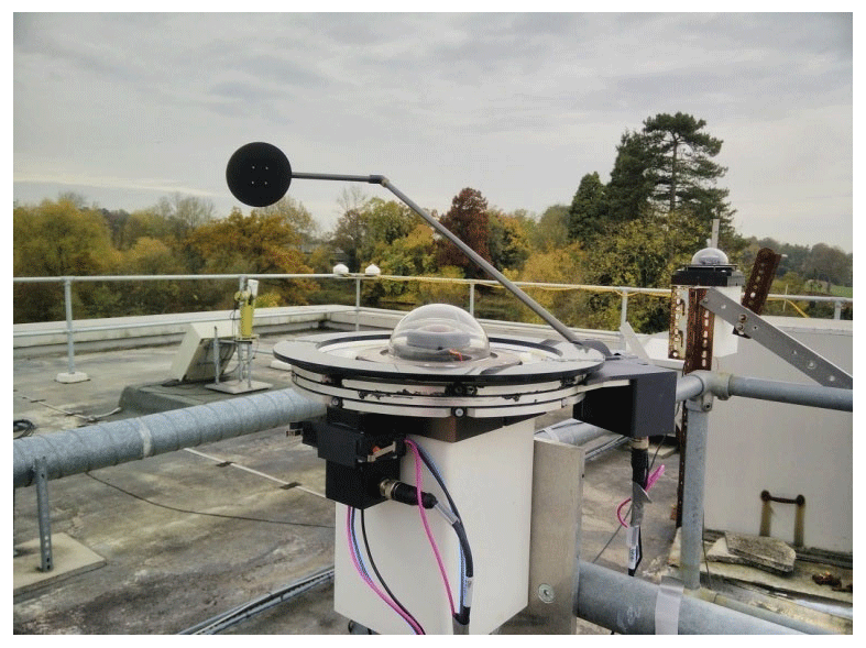
Figure 1All-sky daytime camera with occulting disk in operation in the foreground. The night-time camera is in the background and on the right.
The colour camera has a Bayer mosaic used for filtering the red, blue and green wavelengths. The MATLAB built-in function “demosaic” is applied to the raw image data to reconstruct the full colour image. The fisheye lens enables sky observation over a field of view (FOV) as large as 187∘59′ along the ENE–WSW direction and as large as 142∘38′ along SSE–NNW. The FOV of the daytime camera along ENE–WSW is slightly larger, 189∘53′. The difference is due to the different alignment of the lens relative to the sensor. This is also reflected in the position of the true zenith (x0, y0) with respect to the centre of the camera plane, which for both cameras does not coincide with the true zenith. An offset of 14 pixels in the x direction and 12 pixels in the y direction that corresponds to about 4 and 3.5∘ respectively has been measured for the night-time camera and about 1 and 9.5∘ for the daytime camera. The fisheye lens employed in both cameras uses the “f-theta”, or equidistant projection system, which means that the distance in pixels from the true zenith of the object projected onto the camera plane is simply a scaling factor f (here 3.365 pixels per degree) multiplied by the zenith angle z of the object expressed in degrees (see Sect. 2.2.1). The output images are available either in JPEG or FITS format, but the latter is preferred because of a larger dynamic range and the absence of “digital development” correction.
2.2.1 Camera calibration
Geometric calibration of the camera is done by detecting the position of specific stars and planets in a night-time image and implementing a minimization procedure. This was achieved by using four images, taken at different times of night so that bright stars were available in all quadrants of the image. Over the course of a clear night the daytime camera, whose aperture had been increased from the usual f/16 to f/1.4, was left to take images. Bright star trajectories were plotted as curves on an image, based on their position in the middle of the exposure, the predicted movement and the theoretical f-theta system of the lens. The projection parameters of the camera were then adjusted until the errors between the calculated and true position of the stars on the image were minimized. The procedure will now be described in detail. First, the time the current image was taken was converted to the Julian date. Knowing this time and the longitude and latitude of the camera, the altitude and azimuth of the stars could be calculated from their right ascension and declinations (Meeus, 1999). These coordinates were transformed into the 2-D plane of the image using the f-theta system, found to provide a good initial fit, then were shifted and rotated to account for the fact that the camera does not actually point precisely at the zenith, nor is the image top perfectly aligned with true north. Finally an empirical scaling factor was applied to the coordinates in the x and y direction. With the preliminary f-theta model modified in this way, the camera parameters were manually adjusted until the difference between the plotted stars and their corresponding background star was minimized. The final result was found to align well to the background stars in the central parts of the image and slightly less well around the edges. The equations which map astronomic coordinates into camera ones are
where (z, A) are the zenith and azimuth angles, Δ is the rotation of the camera from north, measuring about 16.4 and 13.6∘ for the night-time and daytime cameras, respectively, (x0, y0) are the pixel coordinates of the actual zenith and f is the scale factor. The latter was found to be 3.365 pixels per degree. If d is the pixel distance from zenith, then the above equations can be rewritten as
The camera characterization just described does not account for lens distortion.
2.2.2 Testing of the lens projection
In order to test the reliability of Eqs. (1) and (2) in reproducing the actual mapping of the lens, the same equations were used to track star and planet trajectories. On a clear night an image was acquired. Given A, z and the acquisition time, pixel coordinates (x, y) of a celestial object can be determined through Eqs. (1) and (2). The actual location is detected by locating the bright spot that corresponds to the star or planet. This is done by selecting an appropriate brightness threshold and converting the image to binary. From the binary image a square region centred where the star/planet is predicted to be (x, y), and sufficiently large to include the spot, is then selected. The centre of mass of the spot then becomes the actual position. Figure 2 shows predicted (blue dots) and actual positions (red dots) of several celestial objects on the night of the 15 February 2013. The mean difference between predicted and actual position was mostly <0.1∘ aside from portions of Vega's, Deneb's, Arcturus', Sirius' and Rigel's trajectories for which larger discrepancies, up to 0.38∘, were observed. These relatively larger deviations are associated with the decreased accuracy of the method due to light pollution, especially significant as the horizon is approached. For these reasons the lens projection was judged to be reasonably well replicated by Eqs. (1) and (2). Consequently, the following image transformations were implemented using exclusively the f-theta system.

Figure 2Predicted (blue dots, from Eqs. 1 and 2) and actual (red dots) star and planet trajectories. Each trajectory is labelled with the name of the star or planet and the mean angular difference between predicted and actual positions.
2.3 Geometric transformations
The SPF is obtained by averaging the image brightness over pixels which are equidistant from the light source (sun or moon) in terms of scattering angle. To achieve this, the raw image is transformed to move the light source to the zenith, to give a light-source-centred system of coordinates. This is accomplished by mapping the original coordinates onto a sphere of unit radius and then by rotating the spherical coordinates to centre the light source at the origin of the final system. The first step consists in changing the projection from “linear” with respect to z to proportional to sin z. Given d, from Eq. (4) z is determined for each pixel (x, y) and the new coordinates (x′, y′) are calculated. The change of projection can be seen as the wrapping of the raw image around a sphere of unit radius with the constraint that the horizon, in the new coordinate system, will now be at a unit distance from the zenith. The periphery of the image which is below the horizon (see Fig. 3) is projected in the lower hemisphere, while points above the horizon appear in the upper hemisphere. The projection of the raw image of Fig. 3 in the upper hemisphere is shown in Fig. 4. The new coordinates x′ and y′ determine the Z coordinate: pixels above and below the horizon are associated with positive and negative Z, respectively. A rotation transformation T is then used to rotate the coordinates (x′, y′, Z) of a generic pixel, identified by the vector P, around the unit vector u that is perpendicular to the line linking the true zenith and the light source, by an angle θ equal to the light source zenith angle zsrc (see Fig. 4) according to
With the rotated coordinates (x′′, y′′, Z′) available, the transformed image in the upper hemisphere can be obtained, and an example is shown in Fig. 5. This can be achieved by interpolating the original image into the new coordinates. Pixels that belong to those portions of the image that after rotation would be below the new horizon are in the lower hemisphere, which is not shown here. This should be accounted for if the SPF is to be calculated for all sky pixels and scattering angles available. Nevertheless that portion of the SPF is not necessary for HR calculation purposes and will not be covered here. The interpolated image is ultimately used to calculate the brightness as a function of the scattering angle by averaging over the entire azimuth angle range. Figure 6 (red dashed line) shows the end result corresponding to the raw image from Fig. 3.
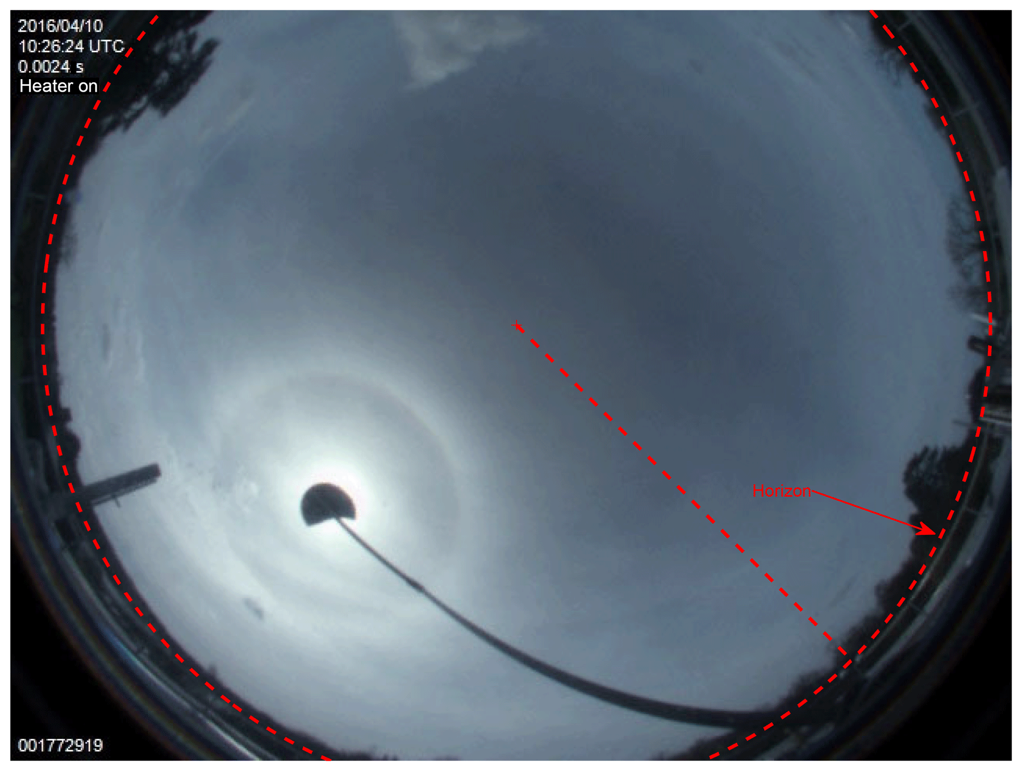
Figure 3All-sky daytime camera image obtained on the 10 April 2016 at 10:26 showing horizon (red solid circle).
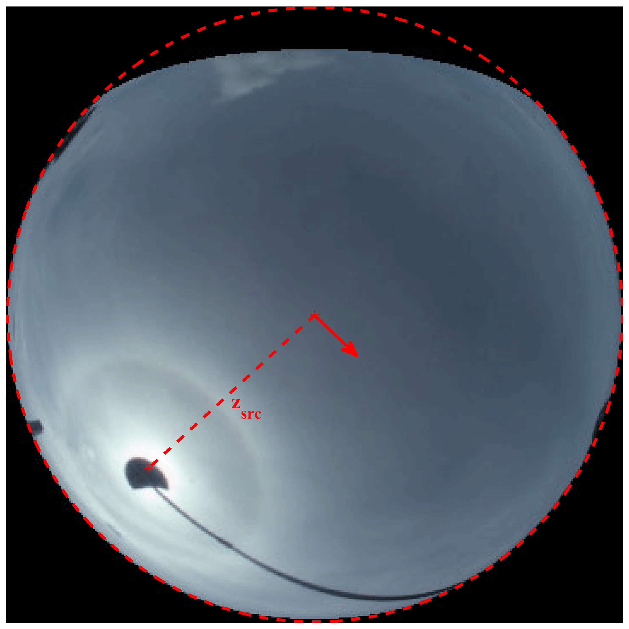
Figure 4Projection of the original image from Fig. 3 onto a sphere (upper hemisphere). The unit vector u determines the direction around which the rotation that leads to the sun-centred image, Fig. 5, takes place; zsrc is the light source zenith angle.
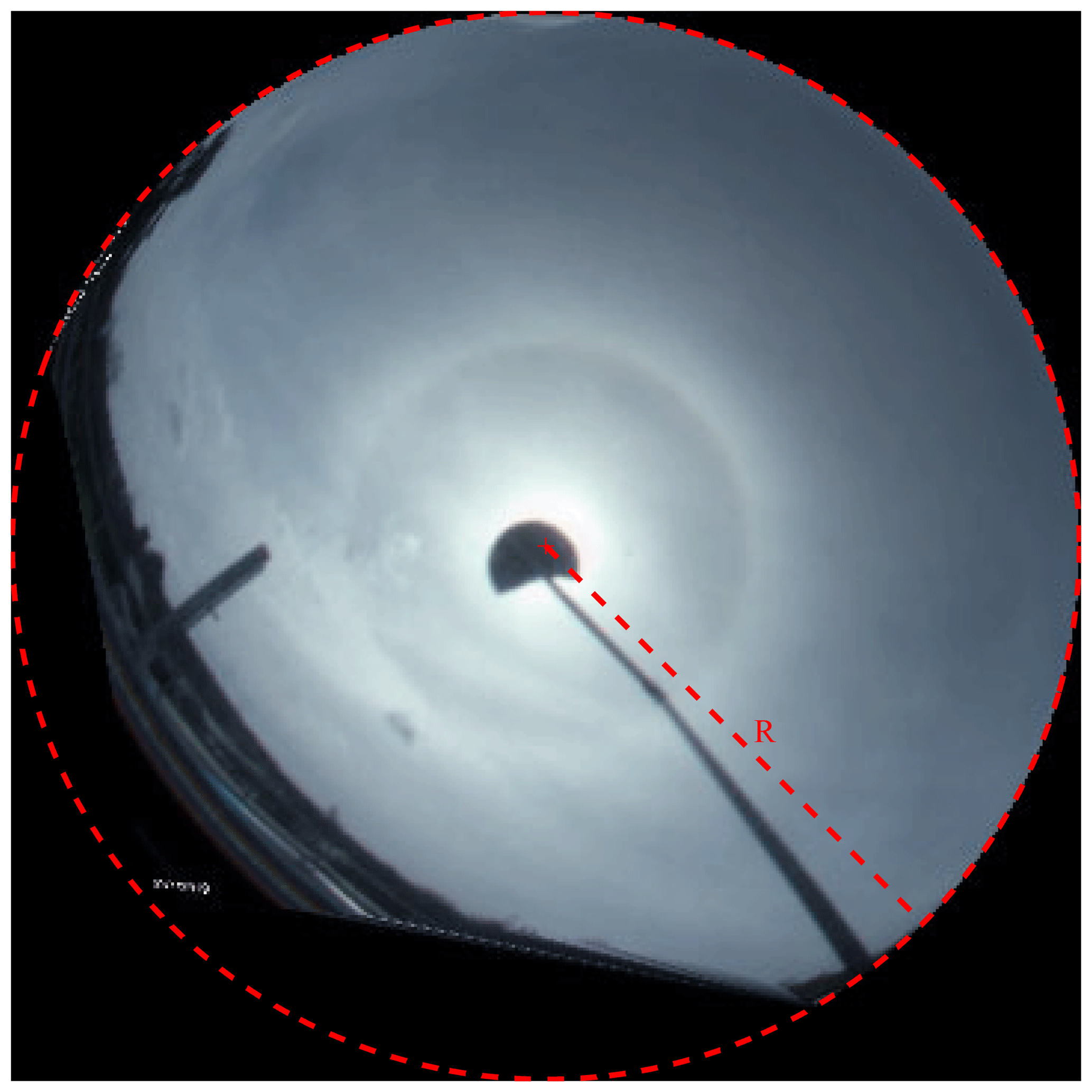
Figure 5Image from Fig. 4 after rotation (upper hemisphere only). R is the radius of the sphere onto which the original images are mapped.
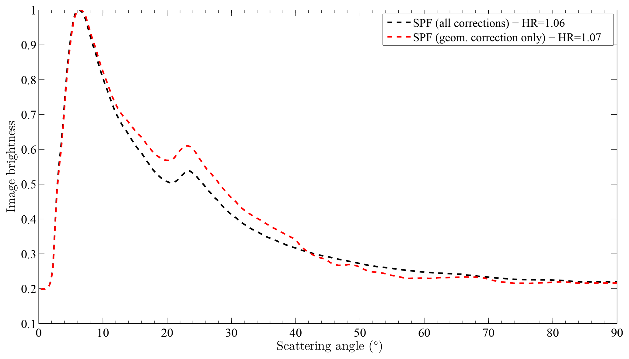
Figure 6Measured scattering phase function corresponding to image in Fig. 3 with geometric correction only (red dashed line) and with geometric, air mass, mask and vignetting corrections (black dashed line). The corresponding HR measures are also shown.
2.4 Background mask
To prevent the contamination of the sky image by background objects above the horizon, a mask, derived from a summer time image, when vegetation is thicker, was used. To prevent the mask edge from falling within the region of the SPF (between 18 and 22∘) from which the HR is derived, only images with zsrc<65∘ were used.
2.5 Vignetting correction
The fall-off of brightness for increasing z, associated with vignetting, takes place in nearly every digital photograph, in all optical lens systems, in particular wide-angle and ultra-wide-angle lenses like fisheye lenses (Jacobs and Wilson, 2007). Optical and natural vignetting are associated with a smaller lens opening for obliquely incident light and the cos 4 law of illumination falloff, respectively, both inherent to any lens design (Ray, 2002). In general, vignetting increases with the aperture and decreases with the focal length. Here it is quantified by comparing daytime image data with sun photometer data under clear sky. While the camera is affected by vignetting, the sun photometer is not; hence the ratio of the corresponding radiance measures, over a similar spectral range, can be used to quantify vignetting. The blue channel of a clear-sky daytime RGB image, with a peak wavelength of 0.46 µm, was extracted (TRUESENSE imaging, 2012), as it provides the best match to the spectral channels of the sun photometer (1.0205, 1.6385, 0.8682, 0.6764, 0.5015, 0.4403 µm) and has larger quantum efficiency and narrower spectral width than the green and red channels. A single sun photometer measurement along the solar principal plane, performed over the various wavelengths, one at a time, about 35 s apart, was compared to the corresponding image brightness from the closest camera measurement (see Fig. 7); as vignetting is assumed to be symmetric under rotations around the camera zenith, pixels such that z is greater than approximately 20∘ over the meridian containing the sun were neglected, and the mean of the sun photometer sky brightness at the visible wavelengths of 0.5015 and 0.4403 µm was smoothed and fitted according to LOWESS (locally weighted scatterplot smoothing). Analogously a polynomial was fitted to the LOWESS smoothed image data. The ratio between the two fitting polynomials (camera to sun photometer) after normalization (see Fig. 8) is what we refer to as the devignetting coefficient (DC; see Fig. 9, black curve). As the DC was expected to be monotonically decreasing with z, the shift of the maximum from the zenith to the position at roughly 8∘ was investigated. This shift was systematically observed for all data. Since the use of the occulting disk allows us to exclude stray light being the cause of it, the simplest explanation comes from observing that such an offset, corresponding to around 27 pixels, corresponds to a displacement of only 0.2 mm between the lens axis and the centre of the aperture. To form a correction function symmetric about the zenith, the original curve was “mirrored” about the zenith (see Fig. 9, red curve), then a Gaussian of the form shown in Eq. (5) was fitted to the mean of the original and the mirror curve (see Fig. 9, dashed curve).
A, B and C obtained in this way are 0.74, 0.26 and 40.03, respectively. The fitting curve provides a working approximation of the actual DC. Figure 6 (black dashed line) shows the SPF corresponding to the raw image from Fig. 3 when geometric, air mass (AM), vignetting and mask corrections are included. The latter removes the contamination associated with objects in the field of view, such as trees, by excluding non-sky pixels from the azimuthal average.
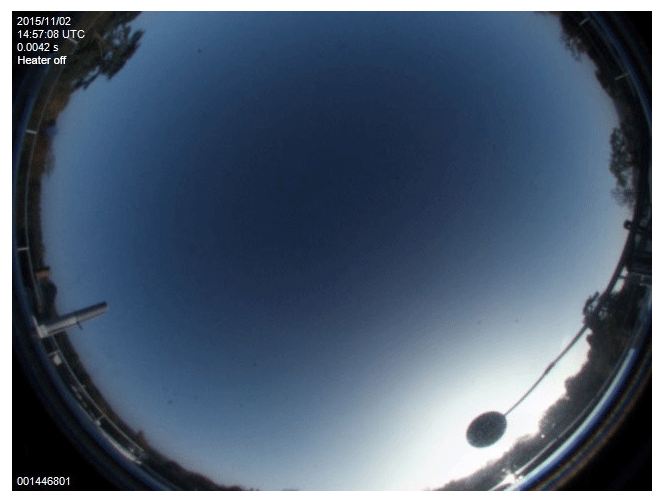
Figure 7Bayfordbury all-sky daytime sky image used for vignetting correction, 11 February 2015, 14:57.
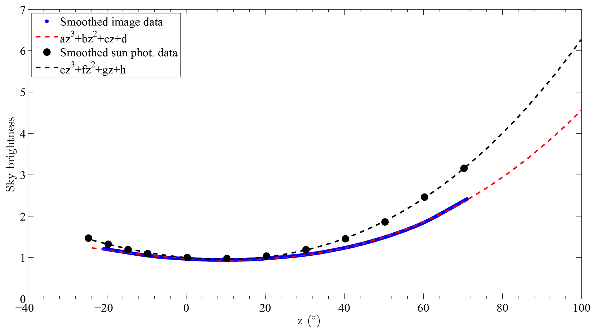
Figure 8All-sky camera and sun photometer normalized fitting polynomials (black dashed line – sun photometer, red dashed line – camera).
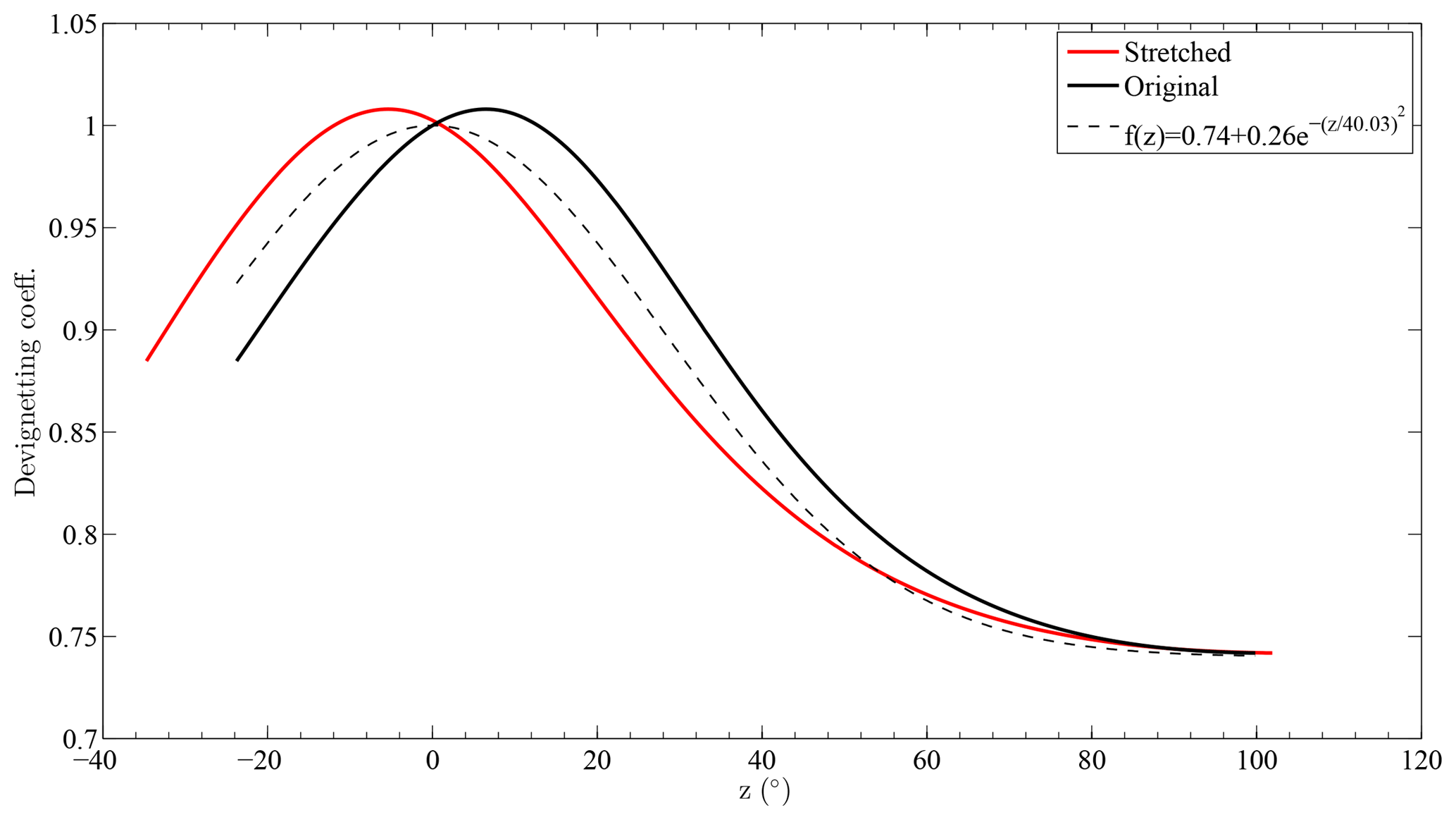
Figure 9Devignetting coefficient: black line – original data, red line – mirrored curve, dashed line – fit.
The vignetting correction obtained this way is intended to be generic. Since the correction is nearly rotationally symmetric, and we have concluded that the residual asymmetry is the outcome of a small misalignment of the sensor, which is likely to vary between cameras, the generic, symmetric correction can be applied to sites where deriving a camera-specific correction is not possible due to the absence of a sun photometer.
2.6 Air mass correction
The additional scattering that light undergoes for slant paths is associated with increased image brightness, evident for large z. While recent sky imaging work neglects it (Forster et al., 2017), such correction is consistent with sky observations (Volz, 1987; Patat, 2003). In this context we will be assuming single scattering approximation, as justified by co-located non-cloud-screened AERONET measurements showing optical thickness <1. To model relative AM, the ratio of the absolute optical air mass M calculated along z to the zenith air mass M0, a non-refracting homogeneous radially symmetric atmosphere was assumed. This provides realistic values of AM near the horizon, where it is less than 40 as is expected (see Table 1 in Rapp-Arraras and Domingo-Santos, 2011). Equation (7) from the same work was used. Such a functional form has already been used for atmospheres with elevated aerosol layers (Vollmer and Gedzelman, 2006). Each pixel brightness was then corrected by dividing it by the corresponding AM(z). With this correction in place, averaging of sky brightness along lines of constant scattering angle becomes possible. However, a sudden drop in the value of the SPF towards large scattering angles was observed, ascribable to the large value that the AM takes for large zenith angles and causing the image brightness to drop rapidly. By excluding such pixels, this unwanted drop is significantly reduced. Moreover, it has been shown previously through radiative transfer calculations accounting for multiple scattering that the brightness of the lower part of the halo reaches a maximum for smaller cloud optical thickness τ than the portion above the sun (Gedzelman and Vollmer, 2008). Consequently, for low solar elevations, a zenith cut-off angle that is too large can cause the HR to decrease due to multiple scattering affecting the part of the halo below the sun. By setting the cut-off at z=70∘, the SPF becomes smooth and multiple scattering effects are reduced while avoiding seasonal bias due to the solar zsrc range covered during the year.
2.7 Cirrus discrimination
A quantification of the temporal fluctuations of the infrared brightness temperature (BT) is expressed in terms of the fluctuation coefficient (FC). The FC is obtained here through detrended fluctuation analysis (DFA) of the BT and is expressed as the exponent of the DFA function following a simple power law (Brocard et al., 2011). It allows the presence of clouds to be detected, unless very thin optically. In fact BT fluctuates significantly under optically thick clouds, while under clear sky it follows the relatively slow-changing water vapour diurnal cycle. Therefore clear-sky FC allows a threshold (DFA threshold) to be set for the transition from clear to cloudy sky. This threshold was chosen empirically to be 0.02 on the basis of the DFA output calculated, unlike in Brocard et al. (2011), every 5 min, over data sampled with 1 s resolution and for time intervals ranging between 20 and 60 s. The intervals were chosen as the time range over which the DFA function was relatively stable and the slope of the function (the FC) was as sensitive as possible to the presence of clouds. The DFA algorithm was applied to 1 year of data, and the corresponding FC time series was averaged over clear-sky periods to set the DFA threshold. This was obtained after manual cloud screening of images associated with minima of the fluctuation coefficient. Furthermore, we wish to point out that like in Brocard et al. (2011) the initial analysis step of cumulative summation (integration) of the time series was not carried out. We note that cumulative summation of a self-affine series shifts the FC by +1 (Heneghan and McDarby, 2000), so the threshold applied here would have a value close to 1 if a standard DFA procedure was followed. Separately, a departure from modelled clear-sky BT due to the presence of relatively optically thick cirrus can provide a BT threshold (Ci threshold) that was used for assessing cloud phase. A simple analytical model of downwelling thermal radiation under clear skies was implemented for this purpose. The model uses ground-level air temperature and integrated water vapour path (retrieved locally from GNSS delays) as input parameters to estimate clear-sky BT at the central wavelength of the pyrometer (Dandini, 2016). In order to establish via BT whether warm or cold clouds are present in the field of view of our instrument, an estimate of the departure of BT from clear-sky BT due to cirrus was calculated. We set the maximum possible departure from clear-sky BT attributable to cirrus as the one when the cloud is warmest and optically thick. Warm liquid clouds would certainly determine a departure from clear-sky BT larger than the one due to such cirrus and hence would lend themselves to be discriminated. By assuming an optically thick cirrus (emissivity of 1) at a temperature of −38 ∘C, representative of the upper temperature limit of ice clouds (Heymsfield et al., 2017), an estimate of the irradiance due to the direct emission of cirrus corrected for the atmospheric attenuation and emission was obtained and converted to brightness temperature by inverting Planck's law (see Figs. 11b and 13b, black dashed line). The Ci threshold follows the diurnal water vapour cycle corrected for the attenuated contribution of such thick cirrus. Above this threshold we can expect optically thick clouds warmer than −38 ∘C, i.e. theoretically not cirrus. Hence, HR time series corresponding to two test cases discussed in the coming section are complemented by simultaneous comparisons of BT with the Ci threshold and the FC with the DFA threshold, as well as broadband downwelling irradiance I. Validation of the presented Ci threshold method is beyond the scope of the present study but will be the subject of a future publication.
We now contrast two case studies based on two consecutive days of observations. Halo ratio time series were obtained on 6 July 2016 between 08:00 and 11:00, when halo and non-halo cirrus alternated with scattered cumuli (see Fig. 10) and on 7 July 2016 between 12:00 and 15:00, when mostly cirrus occurred (see Fig. 12). All-sky images corresponding to HR minima and maxima are shown as insets in the figures. Arrows, specifying the time the image was acquired, are black if the halo is either absent or faint, and yellow otherwise. In variance from the previous definitions of the HR (see Introduction), it was determined as the ratio of the SPF at slightly larger angles: 23 and 20∘, which correspond to the locations of the maximum and minimum we typically found in the measured SPF, respectively. This finding corroborates that of Lynch et al. (1985), who observed these values to be 22.8 and 19.7∘, respectively. This change resulted in enhanced sensitivity of the HR to the halo status of cirrus (see Figs. 11a and 13a). The shift of the halo peak towards larger angles than the 22∘ shown by the more familiar single-scattering SPF computed from geometric optics can be interpreted as originating from the combined contributions from background sky scattering, diffraction effects (due to small crystal size) and crystal roughness (Macke et al., 1996; Ulanowski, 2005; Liu et al., 2013; Smith et al., 2015). The SPF was obtained by taking the mean of the three camera channels. This was done because most all-sky cameras of the type described here are greyscale.
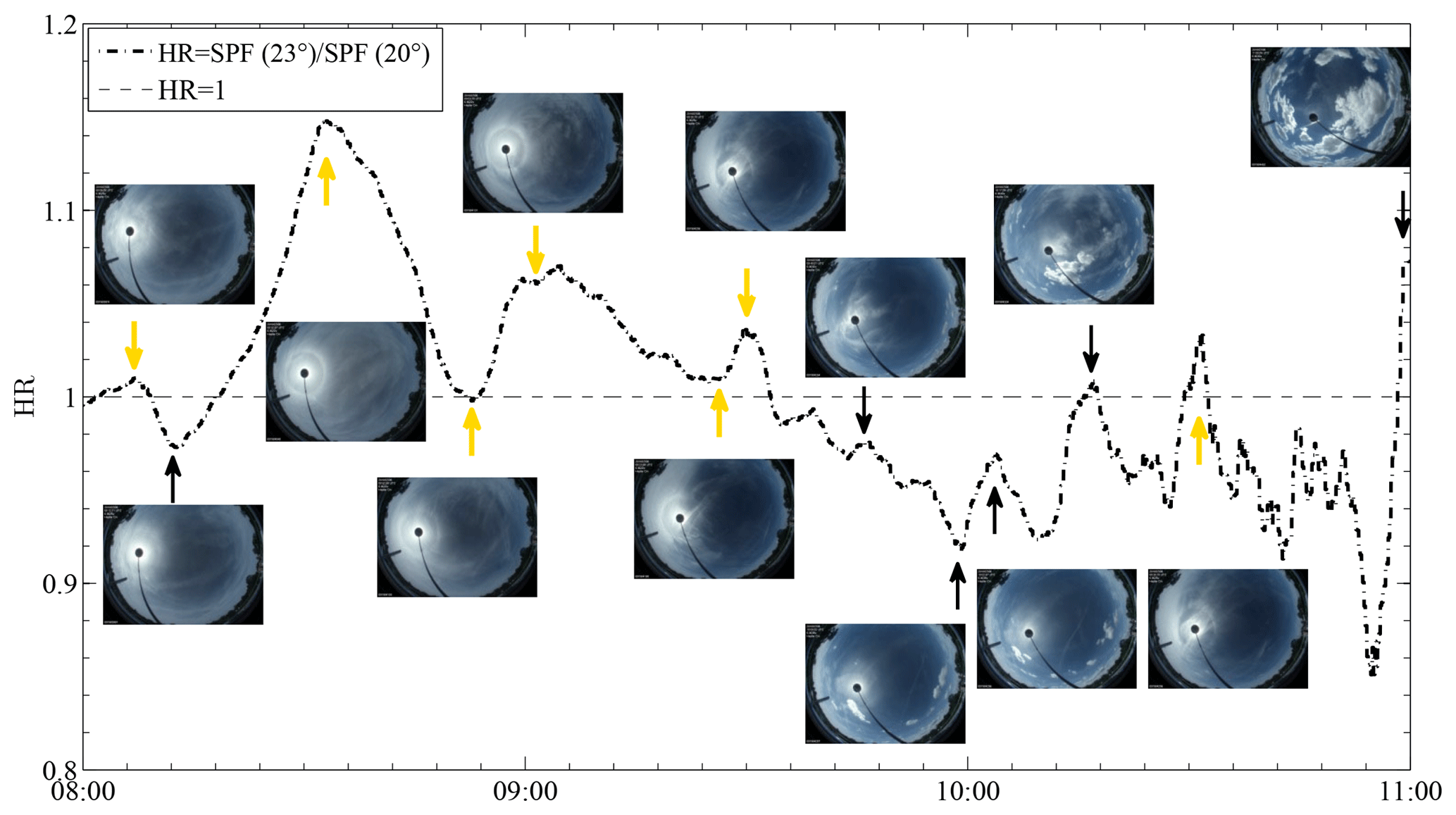
Figure 10HR time series from 6 July 2016 between 08:00 and 11:00. All-sky images corresponding to peaks and dips are also shown. Yellow arrows indicate the presence of relatively bright halo, while black ones indicate either the presence of faint halo or the absence of it.

Figure 11Time series from 6 July 2016 between 08:00 and 11:00. (a) HR (halo ratio), black line – new definition, red line – standard formula – (see text). (b) BT (brightness temperature) – black line, FC (fluctuation coefficient) – red dot, DFA (detrended fluctuation analysis) threshold – red dashed line, Ci (cirrus) threshold – black dashed line. (c) Solar irradiance.
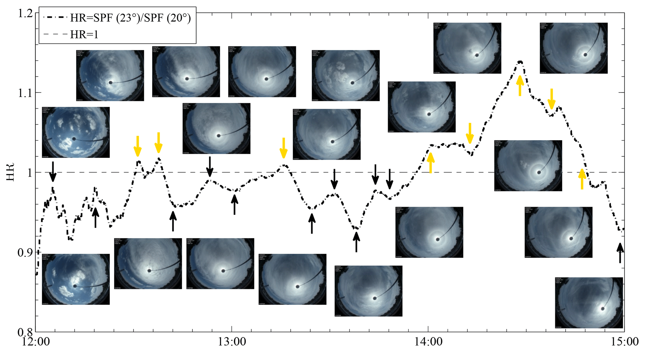

Figure 13Time series from 7 July 2016 between 12:00 and 15:00. (a) HR (halo ratio), black line – new definition, red line – standard formula – (see text). (b) BT (brightness temperature) – black line, FC (fluctuation coefficient) – red dot, DFA (detrended fluctuation analysis) threshold – red dashed line, Ci (cirrus) threshold – black dashed line. (c) Solar irradiance.
3.1 Test case 1: 6 July 2016
On 6 July between 08:00 and 10:00, cirrus occurs as all-sky camera, BT observations and FC measures all show (see Fig. 11). The FC is nearly always above the DFA threshold, while the BT is below the Ci threshold. Over this time window, on qualitative grounds, the behaviour of the BT and the solar irradiance, which in general grows and decreases with τ, respectively, suggests that the HR increases with the optical thickness τ (see Fig. 11b and c). This is consistent with the results of simulations (Kokhanovsky, 2008), based on ray tracing techniques incorporating physical optics (Mishchenko and Macke, 1998) and neglecting molecular and aerosol scattering, that show a linear increase of halo brightness with increasing τ up to τ=3 and a decrease for τ>3 due to multiple scattering. Between about 08:00 and 08:20, the HR, mostly <1, shows a maximum and a minimum at about 08:06 and 08:12, respectively, when a relatively faint 22∘ halo is visible. Maxima with HR >1, on the other hand, are measured at 08:33 and 09:06, when bright halo is observed, and at 09:30, when lower halo brightness is associated with decreased HR. Similarly, the attenuated halo brightness at about 8:51 corresponds to an HR minimum. Between 09:36 and 10:00 the HR drops below 1, and cirrus gets thinner. The small local maxima observed over the same time window at about 09:38, 09:45 and 09:54 are ascribable to cirrus optical depth variations. From 10:00, as cirrus disperse, cumuli start entering the field of view of the camera. A local HR maximum is then measured at 10:03, whereas HR values are >1 at 10:16, 10:33 and 11:00, while scattered cumuli over a mostly clear background increasingly occur. The FC testifies to the presence of clouds, whereas the BT becomes larger than the Ci threshold only at about 10:54, probably because of the sparse nature of the cumuli preventing significant direct radiation from falling within the field of view of the radiometer. However, dips of the solar irradiance I at approximately 10:24, 10:32 and 10:42, indicating increased optical depth, are also observed. While on an overcast day global irradiance depends primarily on diffuse irradiance (Kaskaoutis et al., 2008), on a partly cloudy day clouds crossing the sun path are the main factor to determine variations in the signal of the pyranometer. In particular the ratio of diffuse to global irradiance has been estimated to be 0.15, 1 and >0.15 under clear, overcast and partly cloudy sky, respectively (Duchon and O'Malley, 1999; Orsini et al., 2002). These relatively large HR values are artefacts caused by the image becoming brighter at larger scattering angles, possibly due to bright cloud edges. Such cases should be screened out from the analysis as the HR parameter applies to ice clouds only. This example shows that while a relatively large HR (HR >1) can be an indication of the presence of halo-producing cirrus, this does not always have to be the case.
3.2 Test case 2: 7 July 2016
On 7 July between 12:00 and 15:00 the sky is mainly characterized by the presence of cirrus, except between about 12:00 and 12:30 when sparse cumuli are seen, around 12:45 when relatively opaque altocumuli occur, between around 13:30 and 13:48 and about 14:15 when cumuli overlap with the cirrus background (see Fig. 12). Correspondingly, the FC is always above the DFA threshold, while the BT is mostly below the Ci threshold, although larger values are observed at about 12:20, 12:27, 12:42, 12:48, 13:40, 14:15 and 14:18 when, as expected, the solar irradiance I drops. The HR peaks measured at about 12:06 and 12:18, in similarity with the previous case, appear to be associated with bright cloud edges. Between 12:30 and 12:38, when bright halo is visible, the HR is >1 and then decreases until about 12:42 by which time the halo is no longer visible, possibly due to multiple scattering associated with the increased τ, as demonstrated by the decreased solar irradiance at that point (Fig. 13). With halo-producing cirrus present again from 12:50, the HR increases, except for a local minimum at about 13:00, until about 13:18, when it becomes larger than 1 and the halo is correspondingly sharper. The HR then drops fairly steadily, except for a local maximum at about 13:30, while the halo, still partly visible, fades gradually away to eventually disappear by about 13:36. This is when, we hypothesize, cloud τ has become <1 and Rayleigh and aerosol scattering contribute to the halo contrast reduction. A faint halo present from about 13:45 gets quite sharp by 14:00 as the HR again becomes larger than 1. The halo brightness then stays constant for about 10 min before the HR reaches another minimum at about 14:12, when cumuli are seen by the camera. As the halo sharpness increases, the HR also increases fairly uniformly until about 14:28, when a maximum of 1.14 is reached. We speculate, based on previous findings (Forster et al., 2017; Kokhanovsky, 2008), that this is when τ, probably somewhere between 1 and 3, becomes significantly larger than Rayleigh and aerosol optical thickness without exceeding the optical depth beyond which multiple scattering becomes dominant. The HR then drops to 1 in less than 20 min, while the halo is still fairly bright, and continues to go down until 15:00, when the halo is eventually no longer visible. Peaks at about 14:40 and 14:54 are due to rapid variations in sky brightness, associated with cumuli like those observed near 14:38, which, in analogy with the minima seen at 14:12 and 14:48, cause the SPF to vary significantly as the cumuli transit over the cirrus. With an average BT roughly 10 ∘C higher than on the previous day, this is a case of relatively warm halo-producing cloud; yet the relatively large HR indicates that the cloud is dominated by ice.
Overall the HR correlates well with the fluctuating halo visibility observed throughout the periods examined. Manual inspection of the all-sky images allows us to state that when the HR >1 the halo is visible 95 % of the time (true positives), while halo visibility associated with HR <1 represents only 10 % of the occurrences (false negatives). This relatively minor fraction may be associated with locally larger values of optical thickness, as the partial cirrus thickening observed in the sky images at 13:00 and 13:24 on the 7 July suggests. According to previous radiative transfer calculations (Forster et al., 2017), we conjecture that in order to observe the absolute HR maxima measured for the two cases discussed here, a certain minimum fraction of smooth hexagonal ice columns had to be present.
A method for the retrieval of the halo ratio HR from all-sky imaging has been proposed. This consists of applying a series of image transformations and corrections needed to interpret images quantitatively in terms of an approximation to the scattering phase function. Halo formation can then be identified by taking a ratio of phase function values at particular scattering angles in the vicinity of the halo peak. Unlike in previous studies which tended to use slightly smaller angles (Auriol et al., 2001; Gayet et al., 2011; Ulanowski et al., 2014; Forster et al., 2017), we have used a ratio at scattering angles of 23 and 20∘ corresponding to the locations of the maximum and minimum we typically found in the measured SPF, respectively. The new angles result in higher values of the HR from our data than the HR definitions cited above. After applying the corrections and transformations, HR time series have been shown for two test cases, 6 and 7 July 2016. HR values ≥1 were observed under halo-producing cirrus but also sometimes under scattered low-level clouds when HR maxima appeared to be artefacts due to bright cloud edges. As previously predicted (Kokhanovsky, 2008) multiple scattering appears to lead to decreased HR. We have partly counteracted this by excluding from the HR calculations pixels at z>70∘. However, in future it would be possible to exclude the lower parts of the halo where the slant optical thickness is too large. This implies having to estimate the cirrus optical thickness τ, which could be derived from pyranometer measurements, for example (Fitzpatrick and Warren, 2005; Qiu, 2006) – allowing us, by the way, to verify the expected relation between HR and τ which sets a maximum HR at τ=1 (Forster et al., 2017). Overall the HR is shown to be sensitive to the halo status of cirrus as it is well correlated with halo visibility, aside from a relatively minor fraction of the data with visible halo and HR <1, possibly associated with locally larger values of optical thickness. All-sky cameras have the advantage of being relatively cheap when compared to more complex and difficult-to-align tracking systems such as the HaloCam (Forster et al., 2017). Moreover like the sun-tracking camera used by Foster et al. (2017), who quantified the shift of the red tinged inner edge of the 22∘ halo, colour all-sky cameras can also provide spectral dependence.
However, the all-sky camera data should also be supplemented with additional information if the HR observations are to be associated only with cirrus: a separate cirrus detection method is necessary to screen out non-ice clouds and clear-sky periods, before deriving reliable HR statistics. The quantification of the fluctuations of the brightness temperature BT, expressed in terms of the fluctuation coefficient FC, has been used to discriminate clouds from clear sky by comparing the FC to the DFA threshold, which is used to set the transition from clear to cloudy skies. However, for very small τ the fluctuations of the BT can be of a similar magnitude as under clear sky, putting a limit on this technique in the context of very thin cirrus. Additionally, an estimate of the magnitude of the BT in the presence of optically thick cirrus has been used as an indicator of cloud phase. This method has managed to detect cirrus most of the time over the periods of observation. However it was unable to discriminate some of the scattered cumuli, sometimes associated with high HR values that have to be screened out from the analysis and in one case failed to confirm the presence of ice, as shown by the presence of the 22∘ halo. When no other sky observations are available and attenuation of solar irradiance due to aerosol can be measured or accounted for, a method previously implemented for solar irradiance time series from pyranometer measurements can be used for cloud classification (Duchon and O'Malley, 1999). This can be achieved by accounting for the standard deviation of the scaled observed irradiance and the ratio of the former to the scaled clear-sky irradiance (Duchon and O'Malley, 1999) or, as a cheap and relatively easy-to-use alternative, by combining observed total irradiance, temperature and relative humidity (Pagès et al., 2003). In the future these cirrus discrimination methods should be compared to techniques such as microwave radiometry or lidar, which would allow us to assess their relative merit. As an alternative to BT radiometry the backscattered signal from lidar can be used to discriminate between cloudy and clear skies. If depolarization information is not available, cloud-phase discrimination can be achieved from cloud base height by estimating cloud base temperature. Such estimates can be improved if temperature profiles are available from radiosonde ascents (Forster et al., 2017). While this has the advantage that the cloud base temperature will be less sensitive to τ than the temperature from the radiometer, on the other hand this method requires additional measurements. However it can be considered an alternative if such measurements are available at the given observation site.
Ultimately, the method proposed here is meant to provide cirrus characterization. The two test cases analysed show the presence of large (compared to wavelength, probably characterized by size parameters larger than 100; Mishchenko and Macke, 1999) and regular, smooth ice crystals. Results of previous investigations (Forster et al., 2017) have been used to speculate on such smooth crystal fraction. We argue that when the 22∘ halo was visible, a significant percentage of regular ice crystals had to be present and that such a fraction is likely to have been much larger when the HR reached its absolute maxima. The remaining fraction could have been composed of irregularly shaped, complex, rough or small ice crystals.
Long-term observations of halo displays, preferably at multiple sites, must be carried out to allow statistics of the occurrence of halo-producing cirrus, which still remains unknown, to be obtained. The magnitude of the HR could then be used to assess aspects of the composition of the cirrus – while remembering that a low HR can have multiple causes, as discussed above. Furthermore, by extending the method to additional halo displays, further information on ice crystal geometry could potentially be obtained; e.g. the presence of sun dogs and the 46∘ halo indicates the presence of aligned plates and non-aligned, solid hexagonal prisms, respectively.
The utilization of the all-sky cameras to transform the measured light intensity into an approximation to the scattering phase function and, to a limited extent, the cirrus detection algorithm, are the particularly novel aspects of this work; this has not been done previously to the best of our knowledge. The method applied to the all-sky images in particular, allowing the measurement of the distribution of sky radiance, permits the large field of view associated with the all-sky imaging to be taken advantage of in a quantitative manner. Consequently, while not computationally demanding and relatively easy to implement, this method allows the range of application of all-sky imaging to be broadened beyond the more qualitative recording of cloud fields and optical displays associated with cirrus. The cloud classification method, on the other hand, is original in that it relies on a non-fixed, non-location-specific and easy-to-model temperature threshold. The combined use of these two methods allows relatively inexpensive halo observations and the retrieval of information pertaining to ice particle size and texture. If implemented at multiple locations, the methods can provide a useful dataset for improving the understanding of cirrus composition.
The all-sky camera images are archived on the observatory website at http://observatory.herts.ac.uk/allsky/ (last access: 27 February 2019). Experimental and model data are available from the authors upon request.
PD carried out the data analysis with assistance from ZU. The latter conceived and supervised the project while providing crystal property interpretation of geometric, air mass and vignetting corrections for phase function retrieval. PD implemented the main conceptual ideas and the technical details of the corrections. PD and ZU wrote the paper. RK designed and built the occulting disk while DC installed and automated the occulting shade for sun tracking and provided support in terms of camera calibration and data access.
The authors declare that they have no conflict of interest.
The services of the Natural Environment Research Council (NERC) British Isles
continuous GNSS Facility (BIGF), http://www.bigf.ac.uk (last access: 4 January 2019), in providing archived GNSS
products to this study, are gratefully acknowledged. We thank Paul Kaye
for his contribution to designing the occulting disc and Evelyn Hesse
(University of Hertfordshire) and Anthony Baran (Met Office) for their
valuable advice. Zbigniew Ulanowski acknowledges support from the Natural
Environment Research Council grant NE/I020067/1.
Edited by: Bernhard Mayer
Reviewed by: two anonymous referees
Allmen, M. and Kegelmeyer Jr., W. P.: The computation of cloud-base height from paired whole-sky imaging cameras, J. Atmos. Ocean. Tech., 13, 97–113, https://doi.org/10.1175/1520-0426(1996)013<0097:TCOCBH>2.0.CO;2, 1996.
Auriol, F., Gayet, J. F., Febvre, G., Jourdan, O., Labonnote, L., and Brogniez, G.: In situ observations of cirrus cloud scattering phase function with 22∘ and 46∘ halos: cloud field study on 19 February 1998, J. Atmos. Sci., 58, 3376–3390, https://doi.org/10.1175/1520-0469(2001)058<3376:ISOOCS>2.0.CO;2, 2001.
Baran, A. J.: From the single-scattering properties of ice crystals to climate prediction: A way forward, J. Atmos. Res., 112, 45–69, https://doi.org/10.1016/j.atmosres.2012.04.010, 2012.
Baran, A. J. and Labonnote, L. C.: A self consistent scattering model for cirrus, I: the solar region, Q. J. Roy. Meteor. Soc., 133, 1899–1912, https://doi.org/10.1002/qj.164, 2007.
Baran, A. J., Furtado, K., Labonnote, L.-C., Havemann, S., Thelen, J.-C., and Marenco, F.: On the relationship between the scattering phase function of cirrus and the atmospheric state, Atmos. Chem. Phys., 15, 1105–1127, https://doi.org/10.5194/acp-15-1105-2015, 2015.
Baum, B. A., Yang, P., Heymsfield, A. J., Schmitt, C., Xie, Y., Bansemer, A., Hu, Y. X., and Zhang, Z.: Improvements in shortwave bulk scattering and absorption models for the remote sensing of ice clouds, J. Appl. Meteor. Climatol., 50, 1037–1056, https://doi.org/10.1175/2010JAMC2608.1, 2011.
Berger, L., Besnard, T., Genkova, I., Gillotay, D., Long, C.N., Zanghi, F., Deslondes, J. P., and Perdereau, G.: Image comparison from two cloud cover sensor in infrared and visible spectral regions, in: Proceedings of the 21st International Conference on Interactive Information Processing Systems (IIPS) for Meteorology, Oceanography, and Hydrology, San Diego, CA, 9–13 January 2005.
Brocard, E., Schneebeli, M., and Mätzler, C.: Detection of cirrus clouds using infrared radiometry, IEEE T. Geosci. Remote, 49, 595–602, https://doi.org/10.1109/TGRS.2010.2063033, 2011.
Calbó, J. and Sabburg, J.: Feature extraction from whole-sky groundbased images for cloud-type recognition, J. Atmos. Ocean. Tech., 25, 3–14, https://doi.org/10.1175/2007JTECHA959.1, 2008.
Calbó, J., Pagès, D., and González, J. A.: Empirical studies of cloud effects on UV radiation: a review, Rev. Geophys., 43, 1–28, https://doi.org/10.1029/2004RG000155, 2008.
Campbell, D.: Widefield Imaging at Bayfordbury Observatory, BS thesis, University of Hertfordshire, Hatfield, 47, 2010.
Cazorla, A., Olmo, F. J., and Alados-Arboledas, L.: Using a sky imager for aerosol characterization, Atmos. Environ., 42, 2739–2745, https://doi.org/10.1016/j.atmosenv.2007.06.016, 2008a.
Cazorla, A., Olmo, F. J., and Alados-Arboledas, L.: Development of a sky imager for cloud cover assessment, J. Opt. Soc. Am., 25, 29–39, https://doi.org/10.1364/JOSAA.25.000029, 2008b.
Chow, C. W., Urquhart, B., Dominguez, A., Kleissl, J., Shields, J., and Washom, B.: Intra-hour forecasting with a total sky imager at the UC San Diego solar energy testbed, Sol. Energy, 85, 2881–2893, https://doi.org/10.1016/j.solener.2011.08.025, 2011.
Cimel Electonique, Multiband photometer CE318-N, User's manual, 70 pp., Cimel Electronique, Paris, France, 2015.
Cole, B. H., Yang, P., Baum, B. A., Riedi, J., Labonnote, L. C., Thieuleux, F., and Platnick, S.: Comparison of PARASOL observations with polarized reflectances simulated using different ice habit mixtures, J. Appl. Meteorol. Clim., 52, 186–196, https://doi.org/10.1175/JAMC-D-12-097.1, 2013.
Dandini, P.: Cirrus occurrence and properties determined from ground-based remote sensing, PhD, University of Hertfordshire, Hatfield, UK, 213 pp., 2016.
Duchon, C. E. and O'Malley, M. S.: Estimating cloud type from pyranometer observations, J. App. Meteorol., 38, 132–141, https://doi.org/10.1175/1520-0450(1999)038<0132:ECTFPO>2.0.CO;2, 1999.
Fitzpatrick, M. F. and Warren, S. G.: Transmission of solar radiation by clouds over snow and ice surfaces. Part II: Cloud optical depth and shortwave radiative forcing from pyranometer measurements in the Southern Ocean, J. Climate, 18, 4637–4648, https://doi.org/10.1175/JCLI3562.1, 2005.
Forster, L., Seefeldner, M., Wiegner, M., and Mayer, B.: Ice crystal characterization in cirrus clouds: a sun-tracking camera system and automated detection algorithm for halo displays, Atmos. Meas. Tech., 10, 2499–2516, https://doi.org/10.5194/amt-10-2499-2017, 2017.
Garrett, T. J., Hobbs, P. V., and Gerber, H.: Shortwave, single scattering properties of arctic ice clouds, J. Geophys. Res., 106, 15155–15172, https://doi.org/10.1029/2000JD900195, 2001.
Gayet, J.-F., Mioche, G., Shcherbakov, V., Gourbeyre, C., Busen, R., and Minikin, A.: Optical properties of pristine ice crystals in mid-latitude cirrus clouds: a case study during CIRCLE-2 experiment, Atmos. Chem. Phys., 11, 2537–2544, https://doi.org/10.5194/acp-11-2537-2011, 2011.
Gedzelman, S. D. and Vollmer, M.: Atmospheric optical phenomena and radiative transfer, B. Am. Meteorol. Soc., 89, 471–485, https://doi.org/10.1175/BAMS-89-4-471, 2008.
Ghonima, M. S., Urquhart, B., Chow, C. W., Shields, J. E., Cazorla, A., and Kleissl, J.: A method for cloud detection and opacity classification based on ground based sky imagery, Atmos. Meas. Tech., 5, 2881–2892, https://doi.org/10.5194/amt-5-2881-2012, 2012.
Heinle, A., Macke, A., and Srivastav, A.: Automatic cloud classification of whole sky images, Atmos. Meas. Tech., 3, 557–567, https://doi.org/10.5194/amt-3-557-2010, 2010.
Heneghan, C. and McDarby, G.: Establishing the relation between detrended fluctuation analysis and power spectral density analysis for stochastic processes, Phys. Rev. E, 62, 6103–6110, https://doi.org/10.1103/PhysRevE.62.6103, 2000.
Heymsfield, A., Kramer, M., Brown, P., Cziczo, D., Franklin, C., Lawson, P., Lohmann, U., Luebke, A., McFarquhar, G. M., and Ulanowski, Z.: Cirrus clouds, Meteor. Monographs, 58, 2.1–2.26, https://doi.org/10.1175/AMSMONOGRAPHS-D-16-0010.1, 2017.
Holben, B., Eck, T., Slutsker, I., Tanré, D., Buis, J., Setzer, A., Vermote, E., Reagan, J., Kaufman, Y., Nakajima, T., Lavenu, F., Jankowiak, I., and Smirnov, A.: AERONET – A Federated Instrument Network and Data Archive for Aerosol Characterization, Remote Sens. Environ., 66, 1–16, https://doi.org/10.1016/S0034-4257(98)00031-5, 1998.
Horvath, G., Barta, A., Gal, J., Suhai, B., and Haiman, O.: Ground-based full-sky imaging polarimetry of rapidly changing skies and its use for polarimetric cloud detection, Appl. Optics, 41, 543–559, https://doi.org/10.1364/AO.41.000543, 2002.
Hoyningen-Huene, W., Dinter, T., Kokhanovsky, A., Burrows, J., Wendisch, M., Bierwirth, E., Muller, D., and Diouri, M.: Measurements of desert dust optical characteristic at Porte au Sahara during SAMUM, Tellus B, 61, 206–215, https://doi.org/10.1111/j.1600-0889.2008.00405.x, 2009.
Jacobs, A. and Wilson, M.: Determining lens vignetting with HDR techniques, XII National Conference on Lighting, Varna, Bulgaria, 10–12 June 2007.
Janeiro, F. M., Ramos, P. M., Wagner, F., and Silva, A. M.: Developments of low-cost procedure to estimate cloud base height based on a digital camera, Measurements, 43, 684–689, https://doi.org/10.1016/j.measurement.2010.01.007, 2010.
Johnson, R. W. and Hering, W. S.: Automated cloud cover measurements with a solid state imaging system, Tech. note 206, Visibility Laboratory, University of California, San Diego, Scripps Institution of Oceanography, La Jolla, CA, 11 pp., 1987.
Kaskaoutis, D. G., Kambezidis, H. D., Kharol, S. K., and Badarinath, K. V. S.: The diffuse-to-global spectral irradiance ratio as a cloud-screening technique for radiometric data, J. Atmos. Sol.-Terr. Phy., 70, 1597–1606, https://doi.org/10.1016/j.jastp.2008.04.013, 2008.
Kassianov, E. I., Long, C., and Ovtchinnikov, M.: Cloud sky cover versus cloud fraction: Whole-sky simulations and observations, J. Appl. Meteor., 44, 86–98, https://doi.org/10.1175/JAM-2184.1, 2005.
Kegelmeyer, W. P.: Extraction of Cloud Statistics from Whole Sky Imaging Cameras, SANDIA Report, SAND94-8222, Sandia National Laboratories Albuquerque, New Mexico and Livermore, CA, 17 pp., 1994.
Kokhanovsky, A.: The contrast and brightness of halos in crystalline clouds, Atmos. Res., 89, 110–112, https://doi.org/10.1016/j.atmosres.2007.12.006, 2008.
Korolev, A., Isaac, G. A., and Hallett, J.: Ice particle habits in stratiform clouds, Q. J. Roy. Meteor. Soc., 126, 2873–2902, https://doi.org/10.1002/qj.49712656913, 2000.
Liu, C., Panetta, R. L., and Yang, P.: The effects of surface roughness on the scattering properties of hexagonal columns with sizes from the Rayleigh to the geometric optics regimes, J. Quant. Spectr. Ra., 129, 169–185, https://doi.org/10.1016/j.jqsrt.2013.06.011, 2013.
Long, C. N.: Correcting for circumsolar and near-horizon errors in sky cover retrievals from sky images, The Open Atmos. Sci. J., 4, 45–52, https://doi.org/10.2174/1874282301004010045, 2010.
Long, C. N. and DeLuisi, J. J.: Development of an automated hemispheric sky imager for cloud fraction retrievals, in: Proceedings of the tenth Symposium on meteorological observations and instrumentation, Phoenix, AZ, Amer. Meteor. Soc., 78, 171–174, 1998.
Long, C. N., Slater, D., and Tooman, T.: Total Sky Imager (TSI) Model 880 status and testing results, Tech. Rep., DOE Office of Science Atmospheric Radiation Measurement (ARM) Program, United States, 36 pp., 2001.
Long, C. N., Sabburg, J., Calbó, J., and Pagès, D.: Retrieving cloud characteristics from ground-based daytime color all-sky images, J. Atmos. Ocean. Tech., 23, 633–652, https://doi.org/10.1175/JTECH1875.1, 2006.
Lund, I. A.: Joint probabilities of cloud-free lines of sight through the atmosphere at Grand Forks, Fargo, and Minot, North Dakota, Air Forces Surveys in Geophys., 262, 1–17, 1973.
Lund, I. A., Grantham D. D., and Davis, R. E.: Estimating probabilities of cloud-free field of view from the Earth through the atmosphere, J. Appl. Meteorol., 19, 452–463, https://doi.org/10.1175/1520-0450(1980)019<0452:EPOCFF>2.0.CO;2, 1980.
Lynch, D. K. and Schwartz, P.: Intensity profile of the 22∘ halo, J. Opt. Soc. Am. A, 2, 584–589, https://doi.org/10.1364/JOSAA.2.000584, 1985.
Lyons, R. D.: Computation of height and velocity of clouds over Barbados from a whole-sky camera network, Issue 95 of SMRP research paper, Satellite and Mesometeorology Research Project, University of Chicago, SMRP Research Rep. 95, 18 pp., 1971.
Macke, A., Mueller, J., and Raschke, E.: Single scattering properties of atmospheric ice crystals, J. Atmos. Sci., 53, 2813–2825, https://doi.org/10.1175/1520-0469(1996)053<2813:SSPOAI>2.0.CO;2, 1996.
Martínez-Chico, M., Batlles, F. J., and Bosch, J. L.: Cloud classification in a Mediterranean location using radiation data and sky images, Energy, 36, 4055–4062, https://doi.org/10.1016/j.energy.2011.04.043, 2011.
Meeus, J. H.: Astronomical Algorithms, 2nd edition, Willmann-Bell, Richmond, VA, 477 pp., 1999.
Mishchenko, M. I. and Macke, A.: Incorporation of physical optics effects and computation of the Legendre expansion for ray-tracing phase functions involving δ-function transmission, J. Geophys. Res., 103, 1799–1805, https://doi.org/10.1029/97JD03121, 1998.
Mishchenko, M. I. and Macke, A.: How big should hexagonal ice crystals be to produce halos?, Appl. Optics, 38, 1626–1629, https://doi.org/10.1364/AO.38.001626, 1999.
Orsini, A., Tomas, C., Calzolari, F., Nardino, M., Cacciari, A., and Georgiadis, T.: Cloud cover classification through simultaneous ground-based measurements of solar and infrared radiation, Atmos. Res., 61, 251–275, https://doi.org/10.1016/S0169-8095(02)00003-0, 2002.
Pagès, D., Calbó, J., and González, J. A.: Using routine meteorological data to derive sky conditions, Ann. Geophys., 21, 649–654, https://doi.org/10.5194/angeo-21-649-2003, 2003.
Patat, F.: UBVRI night sky brightness during sunspot maximum at ESO-Paranal, Astron. Astrophys., 400, 1183–1198, https://doi.org/10.1051/0004-6361:20030030, 2003.
Pfister, G., McKenzie, R. L., Liley, J. B., Thomas, A., Forgan, B. W., and Long, C. N.: Cloud coverage based on all-sky imaging and its impact on surface solar irradiance, J. Appl. Meteorol., 42, 1421–1434, https://doi.org/10.1175/1520-0450(2003)042<1421:CCBOAI>2.0.CO;2, 2003.
Qiu, J.: Cloud optical thickness retrievals from ground-based pyranometer measurements, J. Geophys. Res., 111, D22206, https://doi.org/10.1029/2005JD006792, 2006.
Rapp-Arraras, I. and Domingo-Santos, J. M.: Functional forms for approximating the relative optical air mass, J. Geophys. Res., 116, D24308, https://doi.org/10.1029/2011JD016706, 2011.
Ray, S. F.: Applied photographic optics, Focal Press, Oxford, 2002.
Rocks, J. K.: The microscience whole-sky sensor, Fifth Tri-Service Clouds Modelling Workshop, United States Naval Academy, Annapolis, MD, 23–24 June 1987.
Sassen, K., Knight, N. C., Yoshihide, T., and Heymsfield, A. J.: Effects of ice-crystal structure on halo formation: cirrus cloud experimental and ray-tracing modeling studies, Appl. Optics, 33, 4590–4601, https://doi.org/10.1364/AO.33.004590, 1994.
Sassen, K., Zhu, J., and Benson, S.: Midlatitude cirrus cloud climatology from the Facility for Atmospheric Remote Sensing. IV. Optical displays, Appl. Optics, 42, 332–341, https://doi.org/10.1364/AO.42.000332, 2003.
Seiz, G., Baltsavias, E. P., and Gruen, A.: Cloud mapping from the ground: Use of photogrammetric methods. Photogramm. Eng. Rem. S., 68, 941–951, https://doi.org/10.3929/ethz-a-004657107, 2002.
Shaklin, I. A. and Lund, M. D.: Photogrammetrically determined cloud-free lines-of-sight through the atmosphere, J. Appl. Meteorol., 11, 773–782, https://doi.org/10.1175/1520-0450(1972)011<0773:PDCFLO>2.0.CO;2, 1972.
Shaklin, I. A. and Lund, M. D.: Universal methods for estimating cloud-free lines-of-sight through the atmosphere, J. Appl. Meteorol., 12, 28–35, https://doi.org/10.1175/1520-0450(1973)012<0028:UMFEPO>2.0.CO;2, 1973.
Shcherbakov, V.: Why the 46∘ halo is seen far less often than the 22∘ halo?, J. Quant. Spectrosc. Ra., 124, 37–44, https://doi.org/10.1016/j.jqsrt.2013.03.002, 2013.
Shcherbakov, V., Gayet, J. F., Jourdan, O., Strom, J., and Minikin, A.: Light scattering by single ice crystals of cirrus clouds, Geophys. Res. Lett., 33, L15809, https://doi.org/10.1029/2006GL026055, 2006.
Shields, J. E., Koehler, T. L., and Johnson, R. W.: Whole sky imager, in: Proceedings of the Cloud Impacts on DOD Operations and Systems, Marine Physical Laboratory, Scripps Institution of Oceanography, University of California, San Diego, 123–128, 1989/1990.
Shields, J. E., Johnson, R. W., Karr, M. E., Weymouth, R. A., and Sauer, D. S.: Delivery and development of a day/night whole sky imager with enhanced angular alignment for full 24 hour cloud distribution assessment, Final Report, Marine Physical Laboratory, Scripps Institution of Oceanography, University of California, San Diego, 19 pp., 1997.
Shields, J. E., Karr, M. E., Johnson, R. W., and Burden, A. R.: Day/night whole sky imagers for 24-h cloud and sky assessment: history and overview, Appl. Optics, 52, 1605–1616, https://doi.org/10.1364/AO.52.001605, 2013.
Slater, D. W., Long, C. N., and Tooman, T. P.: Total sky imager/whole sky imager cloud fraction comparison, in: Proceedings of the Eleventh ARM Science Team Meeting, Atlanta, Georgia, 19–23 March 2001, 1–11, 2001.
Smith, H. R., Connolly, P. J., Baran, A. J., Hesse, E., Smedley, A. R., and Webb, A. R.: Cloud chamber laboratory investigations into scattering properties of hollow ice particles, J. Quant. Spectrosc. Ra., 157, 106–118, https://doi.org/10.1016/j.jqsrt.2015.02.015, 2015.
Tapakis, R. and Charalambides, A. G.: Equipment and methodologies for cloud detection and classification: A review, Sol. Energy, 95, 392–430, https://doi.org/10.1016/j.solener.2012.11.015, 2013.
TRUESENSE imaging: KAI-0340 Image Sensor 640 (H) × 480 (V) Interline CCD Image Sensor, Rev. 1.0 PS-0024, ON Semiconductor, Phoenix, AZ 85008 USA, 2012.
Ulanowski, Z.: Ice analog halos, Appl. Optics, 44, 5754–5758, https://doi.org/10.1016/j.jqsrt.2005.11.052, 2005.
Ulanowski, Z., Hesse, E., Kaye, P., and Baran, A. J.: Light scattering by complex ice-analogue crystals, J. Quant. Spectrosc. Ra., 100, 382–392, https://doi.org/10.1016/j.jqsrt.2005.11.052, 2006.
Ulanowski, Z., Kaye, P. H., Hirst, E., Greenaway, R. S., Cotton, R. J., Hesse, E., and Collier, C. T.: Incidence of rough and irregular atmospheric ice particles from Small Ice Detector 3 measurements, Atmos. Chem. Phys., 14, 1649–1662, https://doi.org/10.5194/acp-14-1649-2014, 2014.
Um, J. and McFarquhar, G. M.: Dependence of the single-scattering properties of small ice crystals on idealized shape models, Atmos. Chem. Phys., 11, 3159–3171, https://doi.org/10.5194/acp-11-3159-2011, 2011.
Vollmer, M. and Gedzelman, S. D.: Colours of the Sun and Moon: The role of the optical air mass, Eur. J. Phys., 27, 299–309, https://doi.org/10.1088/0143-0807/27/2/013, 2006.
Volz, F. E.: Measurements of the skylight scattering function, Appl. Optics, 26, 4098–4105, https://doi.org/10.1364/AO.26.004098, 1987.
Yi, B., Yang, P., Baum, B. A., L'Ecuyer, T., Oreopoulos, L., Mlawer, E. J., Heymsfield, A. J., and Liou, K. N.: Influence of Ice Particle Surface Roughening on the Global Cloud Radiative Effect, J. Atmos. Sci., 70, 2794–2807, https://doi.org/10.1175/JAS-D-13-020.1,35 2013.