the Creative Commons Attribution 4.0 License.
the Creative Commons Attribution 4.0 License.
 | 01 Mar 2019
Simulation study for ground-based Ku-band microwave observations of ozone and hydroxyl in the polar middle atmosphere
Mark A. Clilverd
Michael Kosch
Annika Seppälä
Pekka T. Verronen
The Ku-band microwave frequencies (10.70–14.25 GHz) overlap emissions from ozone (O3) at 11.072 GHz and hydroxyl radical (OH) at 13.441 GHz. These important chemical species in the polar middle atmosphere respond strongly to high-latitude geomagnetic activity associated with space weather. Atmospheric model calculations predict that energetic electron precipitation (EEP) driven by magnetospheric substorms produces large changes in polar mesospheric O3 and OH. The EEP typically peaks at geomagnetic latitudes of ∼65∘ and evolves rapidly with time longitudinally and over the geomagnetic latitude range 60–80∘. Previous atmospheric modelling studies have shown that during substorms OH abundance can increase by more than an order of magnitude at 64–84 km and mesospheric O3 losses can exceed 50 %. In this work, an atmospheric simulation and retrieval study has been performed to determine the requirements for passive microwave radiometers capable of measuring diurnal variations in O3 and OH profiles from high-latitude Northern Hemisphere and Antarctic locations to verify model predictions. We show that, for a 11.072 GHz radiometer making 6 h spectral measurements with 10 kHz frequency resolution and root-mean-square baseline noise of 1 mK, O3 could be profiled over –0.22 hPa (∼98–58 km) with 10–17 km height resolution and ∼1 ppmv uncertainty. For the equivalent 13.441 GHz measurements with vertical sensor polarisation, OH could be profiled over –0.29 hPa (∼90–56 km) with 10–17 km height resolution and ∼3 ppbv uncertainty. The proposed observations would be highly applicable to studies of EEP, atmospheric dynamics, planetary-scale circulation, chemical transport, and the representation of these processes in polar and global climate models. Such observations would provide a relatively low-cost alternative to increasingly sparse satellite measurements of the polar middle atmosphere, extending long-term data records and also providing “ground truth” calibration data.


1.1 Background information
Energetic particle precipitation (EPP) is an important mechanism in the polar middle and upper atmosphere, causing ionisation in the neutral atmosphere and producing odd nitrogen () and odd hydrogen () (Brasseur and Solomon, 2005; Mironova et al., 2015; Sinnhuber et al., 2012; Verronen and Lehmann, 2013). Enhanced abundances of these chemical species lead to catalytic destruction of ozone (O3) (Jackman and McPeters, 2004), perturbing the radiative balance, dynamics, and large-scale circulation patterns of the atmosphere. This mechanism potentially links solar variability associated with space weather to regional surface climate (e.g. Arsenovic et al., 2016; Baumgartner et al., 2011; Semeniuk et al., 2011; Seppälä et al., 2009, 2013). The energetic particles, mainly protons and electrons of solar and magnetospheric origin, vary widely in energy range and the regions of the atmosphere where they impact, in both geographic–geomagnetic coverage and altitude. Energetic electron precipitation (EEP), with electron energies in the range 20–300 keV, increases ionization in the polar mesosphere at altitudes of 60–90 km (Newnham et al., 2018a; Turunen et al., 2009).
Atmospheric model calculations (Seppälä et al., 2015) predict that EEP driven by magnetospheric substorms produces large changes in polar mesospheric O3 and HOx. The EEP typically peaks at geomagnetic latitudes of ∼65∘ (e.g. Kilpisjärvi, Finland, and Syowa station, Antarctica) and evolves rapidly with time eastwards and over the geomagnetic latitude range 60–80∘ (Cresswell-Moorcock et al., 2013). During the substorms the modelled night-time OH partial column over the altitude range 64–84 km can increase by more than 1000 % and the OH volume mixing ratio (VMR) at 70 km increases from the background (i.e. no substorm) level of ∼8 to ∼60 ppbv (Seppälä et al., 2015). The substorms leave footprints of 5 %–55 % mesospheric O3 loss lasting many hours of local time, with strong altitude and seasonal dependences (Seppälä et al., 2015). The cumulative atmospheric response of ∼1250 substorms yr−1 (Rodger et al., 2016) is potentially more important than the impulsive but highly sporadic (about three to four per year) effects of solar proton events. Other recent studies suggest that EEP from the Earth's outer radiation belt continuously affects the composition of the polar mesosphere through HOx-driven chemistry (Andersson et al., 2014a) and that HOx may cause prolonged mesospheric O3 depletion when NOx is enhanced during polar winter (Verronen and Lehmann, 2015). Mesospheric OH is predominantly produced by the photodissociation of water vapour (H2O) and HOx measurements can also be used as a proxy for mesospheric H2O (Summers et al., 1997). In order to test, verify, and improve models of the polar stratosphere and mesosphere, O3 and OH observations are needed with sufficient precision and time resolution to characterise the different processes that modify their chemical abundances. This paper identifies the instrument characteristics that would be needed to produce the required observations.
1.2 Previous mesospheric ozone and hydroxyl measurements
O3 vertical profiles retrieved in the upper mesosphere (70–100 km) from observations by nine recently operating satellite instruments have been reviewed and compared (Smith et al., 2013). The comparison of coincident profiles showed that upper mesospheric ozone is abundant during the night and depleted during the day, the secondary O3 VMR maximum occurs at 90–92 km during the day and 95 km at night, and O3 VMR is very low (<0.2 ppmv) at about 80 km during both day and night with a minimum in ozone density at sunrise at 80 km. The Microwave Limb Sounder (MLS) on the Aura satellite has provided a long time series of stratospheric and mesospheric O3 measurements (Froidevaux et al., 2008) with global coverage, although the precision of retrieved O3 profiles decreases sharply above 0.1 hPa (∼64 km). MLS observations of mesospheric OH (Pickett et al., 2008) have also helped to elucidate the role of different types of EPP in polar O3 variability (e.g. Andersson et al., 2014b; Verronen et al., 2011; Zawedde et al., 2018). Minschwaner et al. (2011) reviewed OH in the stratosphere and mesosphere and used MLS data to study its diurnal variability. The Spatial Heterodyne Imager for Mesospheric Radicals (SHIMMER) (Englert et al., 2010) measured OH diurnal variations for investigations into discrepancies in mesospheric HOx in photochemical models that had been suggested by earlier satellite observations (Siskind et al., 2013). A major limitation of satellite observations is that the temporal and spatial sampling arising from several overpasses per day at polar locations can make investigating rapidly evolving short-term chemical changes, such as those induced by substorms, a challenge.
Ground-based millimetre-wave radiometry at 110–250 GHz provides continuous measurements of O3 (e.g. Hartogh et al., 2004; Daae et al., 2014; Ryan et al., 2016) and perhydroxyl radical (HO2) (Clancy et al., 1994) but the altitude range is typically restricted to ∼20–75 km. Above ∼75 km, thermal Doppler broadening increases and lower-pressure/higher-altitude information cannot be retrieved from the emission lines. However, for the O3 microwave line centred at 11.072 GHz the atmosphere is much less opaque and Doppler broadening is 10–23 times lower than at 110–250 GHz, allowing the retrieval of O3 VMR to higher altitudes. Low-cost ground-based microwave radiometers operating at 11.072 GHz have been developed using inexpensive Ku-band satellite television low-noise block (LNB) downconverters (Rogers et al., 2009, 2012). Applying a straightforward processing scheme, O3 partial columns for the lower mesosphere (∼50–80 km) and the upper mesosphere–lower thermosphere (∼80–100 km) have been determined from the central 1.25 MHz section of observed 11.072 GHz O3 spectra. The current observations can broadly estimate seasonal O3 variability near the mesopause but would not readily resolve the altitude-dependent O3 changes at 60–90 km that are predicted to occur with substorms. Furthermore, due to the weakness of the 11.072 GHz emission line, measurement times extend to days using a single receiver radiometer achieving a root-mean-square (rms) noise level (1σ) of 5 mK at 9.8 kHz resolution and with 24 h signal integration.
Remote-sensing measurements of mesospheric OH abundances from the ground are challenging due to the low VMR, which typically peaks in the parts per billion by volume range at ∼80 km. Ground-based lidars at mid-latitude sites have detected and identified OH in the ground vibrational state, X2Π (), in the mesosphere at ∼75–85 km altitude (Brinksma et al., 1998a, b). The lidar measurements detect UV resonant fluorescence at ∼308 nm from the OH A2Σ−X2Π electronic transition. In contrast, near-infrared and visible airglow emissions in the X2Π ro-vibrational Meinel system are due to deactivation of vibrationally excited OH* ( to ) generated by the highly exothermic reaction of atomic hydrogen with O3. Satellite measurements of Meinel band nightglow have shown that OH* occurs in a ∼8 km thick layer near 90 km (Zhang and Shepherd, 1999). Ground-based spectroscopic measurements of individual OH vibrational bands in the Meinel emissions can be used to infer temperatures at the mesopause region and estimate relative populations of the v′ states (e.g. von Zahn et al., 1987; Yee et al., 1997; Smith et al., 2010).
1.3 This work
In this work we investigate the potential for measuring diurnal variations in the vertical profiles of O3 in the mesosphere and lower thermosphere using the 11.072 GHz emission line and extending the ground-based microwave radiometry technique to mesospheric OH emissions at ∼13.4 GHz. The microwave spectrum of the most abundant hydroxyl isotopomer, 16OH, at 13.433–13.442 GHz shows four closely spaced lines which arise from the Λ-doubling hyperfine structure in the rotational 2Π3∕2 (v=0, ) state (Radford, 1961; Sastry and Vanderlinde, 1980). The atmospheric OH spectrum is further complicated by the magnetic Zeeman effect, due to the molecule's non-zero total electron spin quantum number (). Each line is Zeeman split into several components polarised in a quasi-symmetric manner and shifted from the central frequency. Here we investigate potential measurements using the most intense of the four OH rotational lines, which has a line position of 13.441 GHz.
The study focuses on atmospheric simulations and retrievals for Kilpisjärvi, Finland, since model data for O3 and OH abundances in substorm and background (no substorm) conditions are available for this location. However, we demonstrate the technique's wider applicability by comparing atmospheric microwave transmittances at six land-based locations including Kilpisjärvi, shown on the maps in Fig. 1. Three potential sites for ground-based instruments are in the Antarctic and three are at high latitudes in the Northern Hemisphere (NH), and all are located close to geomagnetic latitude 65∘ where substorms are predicted to have the greatest effect on mesospheric O3 and OH.
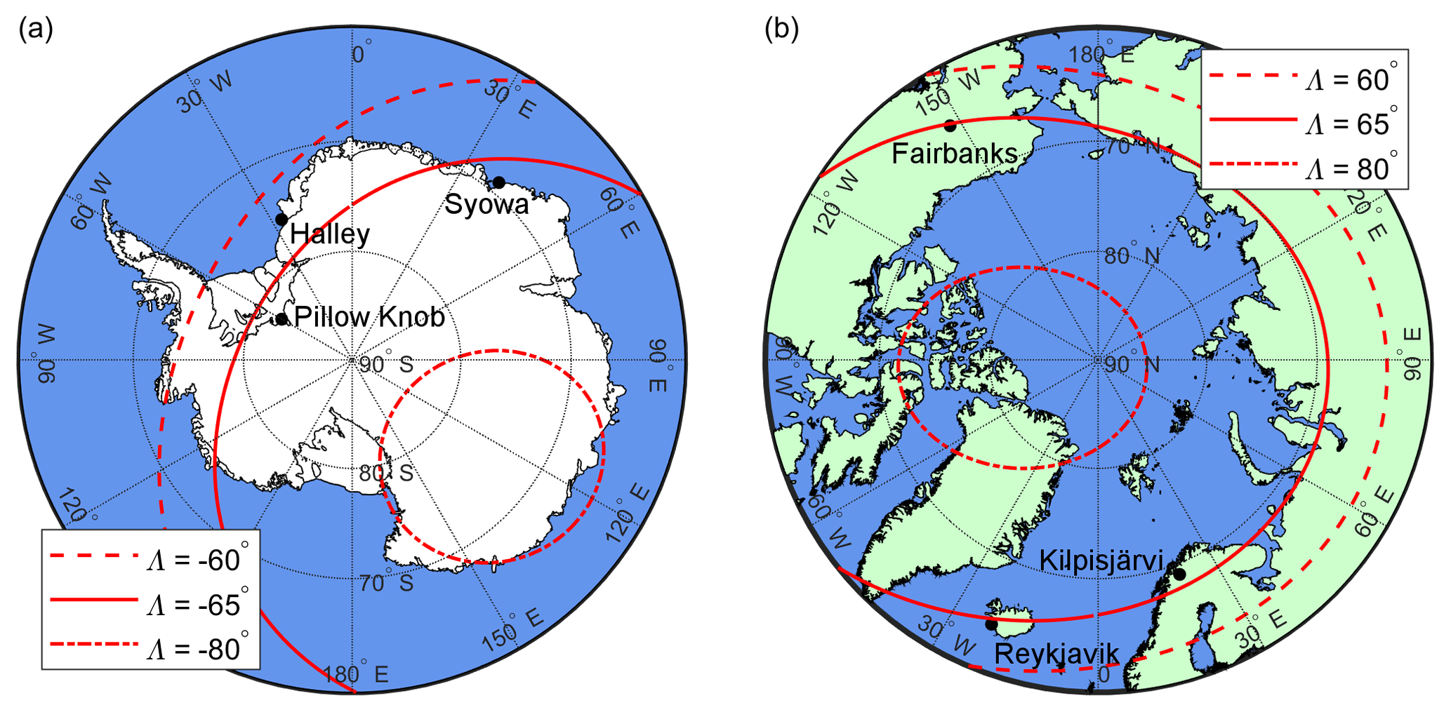
Figure 1Maps of (a) the Southern Hemisphere and Antarctica poleward of geographic latitude 60∘ S and (b) the Northern Hemisphere and Arctic region poleward of geographic latitude 60∘ N. The red dashed, solid, and dotted–dashed lines on each map show the geomagnetic latitudes ∘, ∘, and ∘ respectively, calculated for 1 January 2015 and an altitude of 80 km using the IGRF-12 internal field model (Thébault et al., 2015). Black filled circles indicate the locations of Halley station (75∘37′ S, 26∘15′ W, ∘), Syowa station (69∘00′ S, 39∘35′ E, ∘), and Pillow Knob refuelling station (82∘30′ S, 60∘00′ W, ∘) in (a) and Kilpisjärvi (69∘03′ N, 20∘49′ E, Λ=66.2∘), Finland; Reykjavik (64∘08′ N, 21∘56′ W, Λ=64.4∘), Iceland; and Fairbanks (64∘51′ N, 147∘43′ W, Λ=65.2∘), Alaska, in (b).
Microwave spectrum simulations and retrievals have been performed using atmospheric model datasets in radiative transfer calculations for selected high-latitude and polar locations. The synthesis of VMR profiles at these locations for O3, OH, and seven other atmospheric species, as well as temperature profiles, from available model data is described in Sect. 2.1. The configuration of the radiative transfer forward model for simulating clear-sky atmospheric microwave transmittance and brightness temperature spectra is given in Sect. 2.2, and the setups for performing O3 and OH retrievals for Kilpisjärvi, Finland, are given in Sect. 2.3.
2.1 Atmospheric model datasets
Nine chemical species were identified as significant contributors to the clear-sky atmospheric microwave spectrum in the 11–14 GHz region, overlapping the target O3 and OH lines at 11.072 and 13.441 GHz: ozone (O3), hydroxyl radical (OH), water vapour (H2O), molecular nitrogen (N2), molecular oxygen (O2), perhydroxyl radical (HO2), nitric acid (HNO3), hydrogen peroxide (H2O2), and carbon dioxide (CO2). Monthly mean vertical profiles of VMR for the atmospheric species, and temperature, were calculated using a 10-year dataset from WACCM-D (Verronen et al., 2016) covering 2000–2009. WACCM-D is a 3-D global atmospheric model that incorporates a detailed representation of D-region chemistry in the specified dynamics (SD) version of the Whole Atmosphere Community Climate Model (WACCM 4) (Marsh et al., 2013). The model data were taken from the WACCM-D longitude–latitude grid points closest to the six locations of interest. Seasonal winter mean profiles were calculated using December, January, and February (DJF) data for the NH locations and June, July, and August (JJA) data for the Southern Hemisphere (SH). Similarly, summer mean profiles were calculated using JJA data for the NH locations and DJF data for the SH locations.
O3 and OH VMR profiles for substorm and background (no substorm) conditions were computed by combining data from the 1-D Sodankylä Ion–Neutral Chemistry (SIC) model (Verronen et al., 2005) with monthly mean WACCM-D data. The SIC model data provided VMR data over the altitude range 20–100 km, and monthly mean data from WACCM-D filled the region from the ground up to 20 and above 100 km. Figure 2a shows O3 number density profiles calculated using a 9-day SIC model run (Seppälä et al., 2015) for December 2007 with substorm conditions at Kilpisjärvi. The largest decreases in mesospheric O3 abundance, exceeding 50 %, occur over the altitude range 68–86 m during a 4-day period, after which the number densities return to background levels (Fig. 2b). The percentage changes in O3 partial column over altitudes 64–84 km for the original (15 min) model resolution and 1, 6, and 24 h moving-average smoothed data are shown in Fig. 2c. The three smoothed datasets show reduced diurnal variability compared to the original model data but the largest decrease in O3 partial column is little changed by averaging up to 24 h. VMR profiles for substorm and background (no substorm) conditions were determined from the SIC model data coincident with the largest decrease in O3 partial column, and these and the monthly mean profiles are shown in Fig. 2d. Substorm reductions in O3 VMR occur over the altitude range 64–94 km, with the largest decrease at 72 km.
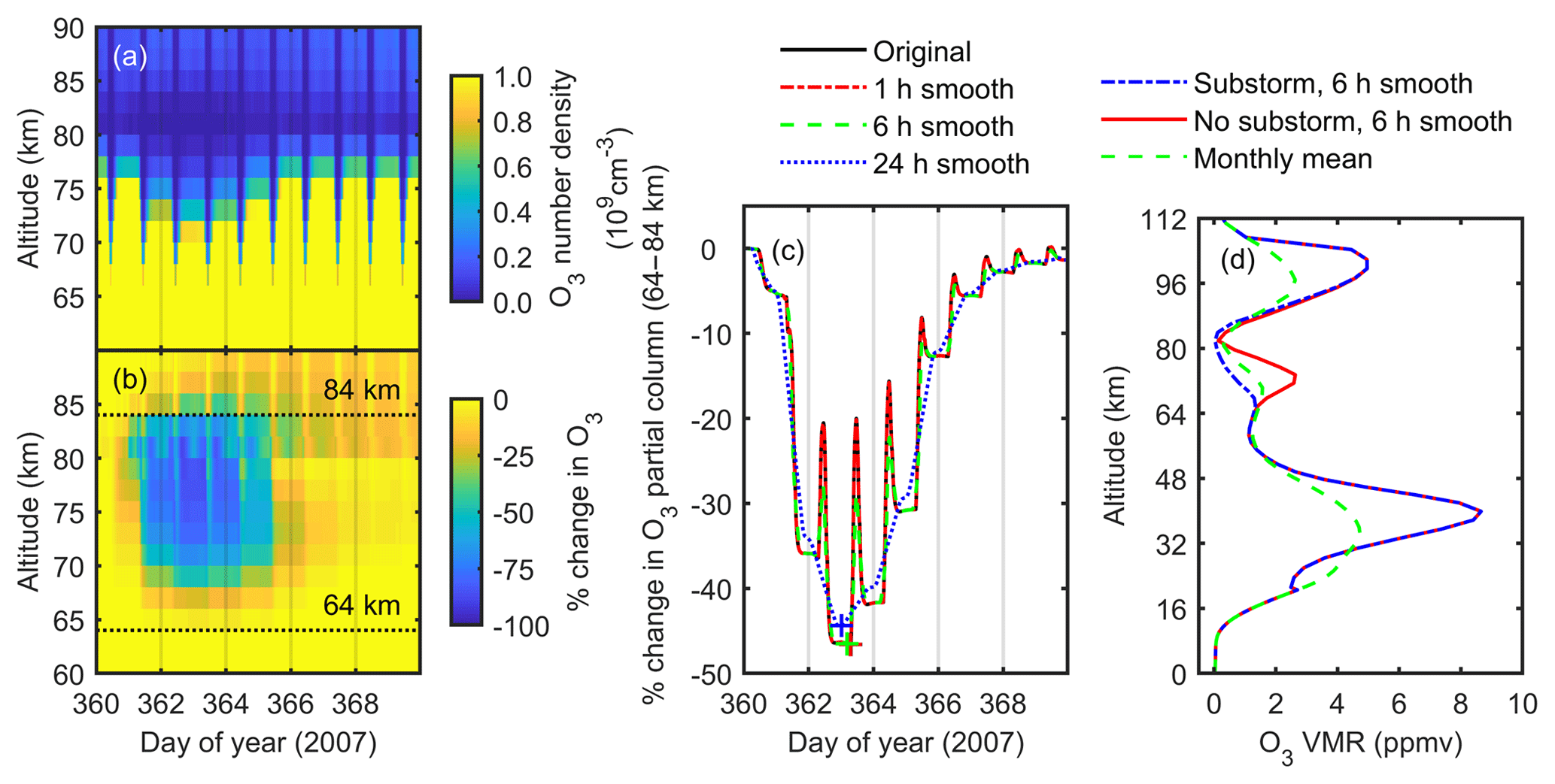
Figure 2Derivation of ozone (O3) volume mixing ratio profiles from atmospheric model datasets. Panel (a) shows O3 number densities calculated by the SIC model for December 2007 substorm conditions at Kilpisjärvi (69∘03′ N, 20∘48′ E), Finland. Panel (b) shows the percentage change in modelled O3 abundance from background (no substorm) conditions. Panel (c) shows the percentage change in O3 partial column over altitudes 64–84 km during substorm conditions for the original (15 min) model resolution and 1, 6, and 24 h smoothed data. “+” symbols indicate the largest decreases in O3 partial column at each nominal time resolution. Panel (d) shows the 6 h smoothed O3 VMR profiles for December substorm, background (no substorm), and monthly mean conditions.
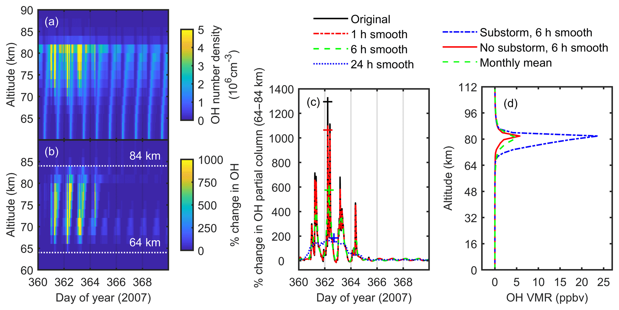
Figure 3Derivation of hydroxyl radical (OH) volume mixing ratio profiles from atmospheric model datasets. Panel (a) shows OH number densities calculated by the SIC model for December 2007 substorm conditions at Kilpisjärvi (69∘03′ N, 20∘48′ E), Finland. Panel (b) shows the percentage change in modelled O3 abundance from background (no substorm) conditions. Panel (c) shows the percentage change in OH partial column over altitudes 64–84 km during substorm conditions for the original (15 min) model resolution and 1, 6, and 24 h smoothed data. “+” symbols indicate the largest increases in OH partial column at each nominal time resolution. Panel (d) shows the 6 h smoothed OH VMR profiles for December substorm, background (no substorm), and monthly mean conditions.
A similar approach was used to determine OH VMR profiles, as shown in Fig. 3. The largest increases in mesospheric OH abundance, exceeding 2 orders of magnitude above the background level, occur at altitudes in the range 66–82 km during the 4 days corresponding to O3 decreases, after which OH number densities return to background levels (Fig. 3a and b). The percentage changes in OH partial column over altitudes 64–84 km for the original (15 min) model resolution and 1, 6, and 24 h moving averages are shown in Fig. 3c. The enhanced level of mesospheric OH during substorms shows greater diurnal variability than the corresponding O3 reductions. Smoothing the modelled OH partial columns significantly reduces the daily maxima, indicating that the improved signal-to-noise ratio from atmospheric measurements longer than ∼6 h would be strongly offset by the smaller integrated OH signal. The 6 h smoothed substorm and background (no substorm) VMR profiles corresponding to the largest decrease in OH partial column, and monthly mean profiles, are shown in Fig. 3d. The substorm profile shows a 5-fold increase in OH VMR around 82 km compared to the monthly mean and background (no substorm) data.
2.2 Forward modelling of atmospheric spectra
Simulated atmospheric microwave spectra were calculated using version 2.2.58 of the Atmospheric Radiative Transfer Simulator (ARTS) (available at http://www.radiativetransfer.org/, last access: 8 August 2016) (Buehler et al., 2005, 2018; Eriksson et al., 2011) and the Qpack2 (a part of atmlab v2.2.0) software package (Eriksson et al., 2005). ARTS is a monochromatic line-by-line model that can simulate radiances from the infrared to the microwave and has been validated against other models in the sub-millimetre spectral range (Melsheimer et al., 2005). The model includes contributions from spectral lines and broadband continua via a choice of user-specified parameterisations. The Planck formalism was used for calculating brightness temperatures and atmospheric transmittance.

Figure 4Pressure-broadened, Doppler-broadened, and Voigt full-width half-maxima (FWHM) line widths for (a) ozone (O3) 11.072 GHz and (b) OH 13.441 GHz emission lines, calculated for mean winter (DJF) and mean summer (JJA) conditions at Kilpisjärvi (69∘03′ N, 20∘48′ E), Finland.
Spectroscopic line parameters for O3, OH, H2O, N2, O2, HO2, HNO3, H2O2, and CO2 were taken from the high-resolution transmission (HITRAN) molecular absorption database (Gordon et al., 2017). For all molecules except OH the Kuntz approximation (Kuntz, 1997) to the Voigt line shape with a Van Vleck–Huber prefactor (Van Vleck and Huber, 1977) and a line cut-off of 750 GHz was used, which is valid for the pressures considered. As the water vapour continuum parameterisation, the Mlawer–Tobin Clough–Kneizys–Davies (MT-CKD) model (version 2.5.2) was used, which includes both foreign and self-broadening components (Mlawer et al., 2012). Collision-induced absorption (CIA) is the main contribution to the dry continua in the microwave range, and therefore the CIA parameterisations from the MT-CKD model (Clough et al., 2005) (version 2.5.2 for N2 and CO2 and version 1.0 for O2) were applied.
In order to compare seasonal atmospheric transmittances at the six different locations, survey spectra over the frequency range 5–20 GHz were calculated at zenith angles of 0 and 82∘ using mean winter and mean summer profiles. A 1 MHz frequency grid was chosen, adequate to characterise smoothly varying broadband transmittance but insufficient to resolve narrowband spectral features.
For simulations of ground-based microwave measurements, values for the frequency resolution, bandwidth, and baseline noise were chosen by considering the range of atmospheric emission line widths and likely instrument performance. Pressure-broadened, Doppler-broadened, and Voigt full-width half-maxima (FWHM) line widths for the lines were calculated using air-broadening coefficients from HITRAN and winter (DJF) and summer (JJA) pressure and temperature profiles at Kilpisjärvi. Figure 4a and b show the variation of O3 11.072 GHz and OH 13.441 GHz line widths with altitude. For both molecules pressure-broadening dominates below ∼90 km, increasing rapidly below 85 km to give FWHM line widths of 300 kHz at ∼65–70 km in winter and ∼70–75 km in summer. Voigt line widths are lowest in the lower thermosphere at ∼95–100 km, with minimum FWHM of 17 kHz for O3 and 34 kHz for OH, and the line widths increase above 100 km due to increased Doppler broadening. Forward model spectra were therefore calculated with a frequency grid spacing of 10 kHz over a bandwidth of 1 MHz to encompass the range of emission line widths from O3 and OH in the mesosphere and lower thermosphere. All measurement simulations were performed for a single pencil beam of radiation at a zenith angle of 82∘.
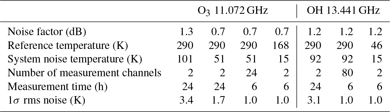
An important consideration in our calculations is that O3 and OH atmospheric spectra can be measured over 6 h with rms baseline noise of 1.0 mK, and this assumption is justified as follows. Low-cost LNB receivers with a noise factor of ∼1.3 dB currently used in O3 11.072 GHz spectrometers for the educational project Mesospheric Ozone System for Atmospheric Investigations in the Classroom (MOSAIC) operate uncooled, i.e. at ambient temperature (Rogers et al., 2012). By analysing signals from both horizontal and vertical polarisation channels of the LNB with 10 kHz frequency resolution, and integrating the atmospheric signal for 24 h, an atmospheric spectrum with baseline noise of ∼3.4 mK is achieved. The statistical fluctuation ΔT (K) in the total system temperature, Tsys (K), is calculated according to the ideal radiometer equation (Kraus, 1986):
where t is observation time (in seconds), Δf is the frequency resolution (in hertz) of the radiometer, and NCH is the number of measurement channels. Applying this equation we can define the sensor characteristics needed to achieve a signal-to-noise ratio of 1.0 mK in 6 h measurements, providing adequate time resolution to observe predicted changes in mesospheric O3 and OH. The results in Table 1 show that higher-performance LNB receivers, with a noise of factor 0.7 dB, would achieve such measurements of the O3 11.072 GHz emission if cooled to 168 K. Alternatively, an array of 12 receivers operating at room temperature, with a total of 24 measurement channels, would achieve this measurement performance. At the higher frequency (13.441 GHz) of the OH emission, available LNBs are less sensitive, with a noise factor of 1.2 dB, and would require cryogenic operation at 46 K to achieve the equivalent performance. A receiver array at room temperature would need 40 spectrometers (i.e. 80 measurement channels) to achieve the required measurement performance at 13.441 GHz. Thus we conclude that suitable receivers could be constructed using commercially available LNB receivers, albeit with the added complexity and higher power consumption needed for low-temperature operation or, alternatively, by combining the outputs from multiple room temperature receivers to achieve higher signal-to-noise spectra.
Table 1Calculated performance for ozone (O3) 11.072 GHz and hydroxyl (OH) 13.441 GHz radiometers with 10 kHz frequency resolution.
The treatment of the Zeeman effect in the Stokes formalism of ARTS is described by Larsson et al. (2014). The Zeeman components of the OH line centred at 13.441 GHz were calculated for an instrument viewing at an azimuthal angle of 0∘ i.e. northward-looking from Kilpisjärvi, with sensor polarisation being vertical, horizontal, or in both directions combined. Magnetic field data were taken from IGRF-11 (Finlay et al., 2010) and the Faddeeva function was used to describe the line shape.
Forward model spectra were calculated for ground-based clear-sky observations during December substorm and background (no substorm) conditions at Kilpisjärvi. The emission signals from different altitudes were found by selectively setting O3 and OH VMR to zero for 10 km sections of the mesosphere and lower thermosphere, and also running simulations with zero O3 and OH VMR at all altitudes. In order to assess measurement uncertainties in the retrieval algorithm and its ability to reproduce the “true” state of the atmosphere, two sets of 500 spectra each of O3 and OH were calculated for Monte Carlo (MC) error analysis. In one set of MC repeat spectra all VMR profiles were kept constant at the true values whereas in the other set the O3, OH, and H2O profiles were randomly scaled using a uniform distribution over the range 0.5–2.0. Baseline noise with a rms level of 1.0 mK was randomly calculated and added to each individual O3 and OH spectrum in both of the MC sets.
2.3 Retrievals
The 6 h atmospheric spectra, simulated for December substorm and background (no substorm) conditions at Kilpisjärvi, were inverted into altitude profiles of O3 and OH VMR using the optimal estimation method (OEM) (Rodgers, 2000) implemented in Qpack (Eriksson et al., 2005). Iterative absorption calculations in ARTS were performed line by line within the radiative transfer calculation, rather than using precalculated look-up tables, in order to accurately model atmospheric spectra (Buehler et al., 2011). VMR values were retrieved for altitude levels 0–120 km with a 1 km spacing, for which hydrostatic equilibrium was assumed for the altitude and pressure. The O3, OH, and H2O a priori VMR profiles were the December monthly mean profiles for Kilpisjärvi. The diagonal elements in the covariance of the O3 and OH a priori VMR profiles were fixed to 1.5 ppmv and 10 ppbv respectively, whereas for H2O they were fixed at the square of 50 % of the VMR values. The off-diagonal elements of the covariance linearly decrease with a correlation length of a fifth of a pressure decade (approximately 3 km).
3.1 Simulated atmospheric spectra
Survey clear-sky atmospheric transmittance spectra, calculated for the selected locations, are shown in Fig. 5. Water vapour absorption leads to decreased transmittance at frequencies above 10 GHz. Higher transmittance occurs for the three colder, desiccated Antarctic sites whereas the generally milder NH locations have lower transmittance, especially in summertime. Considering the frequencies of the O3 and OH lines, at a zenith angle of 0∘, transmittance is 0.98 at the six locations in both winter and summer conditions. At a zenith angle of 82∘ the lower transmittance, in the range 0.84–0.86, is due to the higher air mass factor and increased tropospheric attenuation in particular by water vapour, oxygen, and nitrogen continua. However, the very similar transmittances at various locations suggest that the different seasonal meteorology should have little impact on the proposed O3 and OH observations, unlike ground-based measurements using higher frequencies in the millimetre-wave region where cold, dry, high-altitude sites are advantageous.
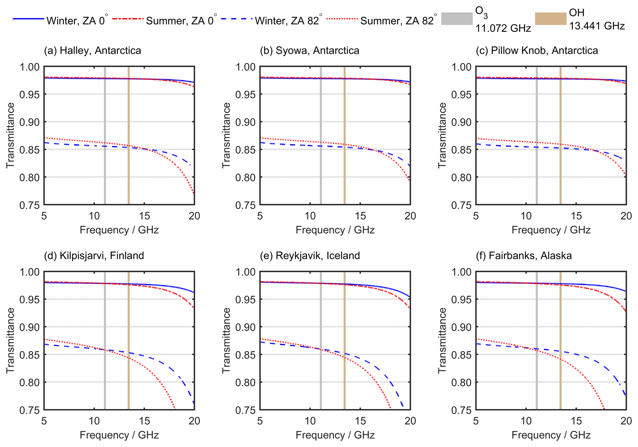
Figure 5Survey atmospheric transmittance spectra at six polar locations for the frequency range 5–20 GHz, calculated on a 1 MHz frequency grid. In panels (a)–(c) transmittances calculated at zenith angles (ZAs) of 0∘ (i.e. viewing vertically upwards) and 82∘ are shown for mean summer (DJF) and mean winter (JJA) conditions at three Antarctic locations. In panels (d)–(f) transmittances calculated at ZAs of 0 and 82∘ are shown for mean summer (JJA) and mean winter (DJF) conditions at three Arctic locations. The light grey and light brown vertical lines indicate the frequencies of the ozone (O3, 11.072 GHz) and hydroxyl (OH, 13.441 GHz) emission lines.
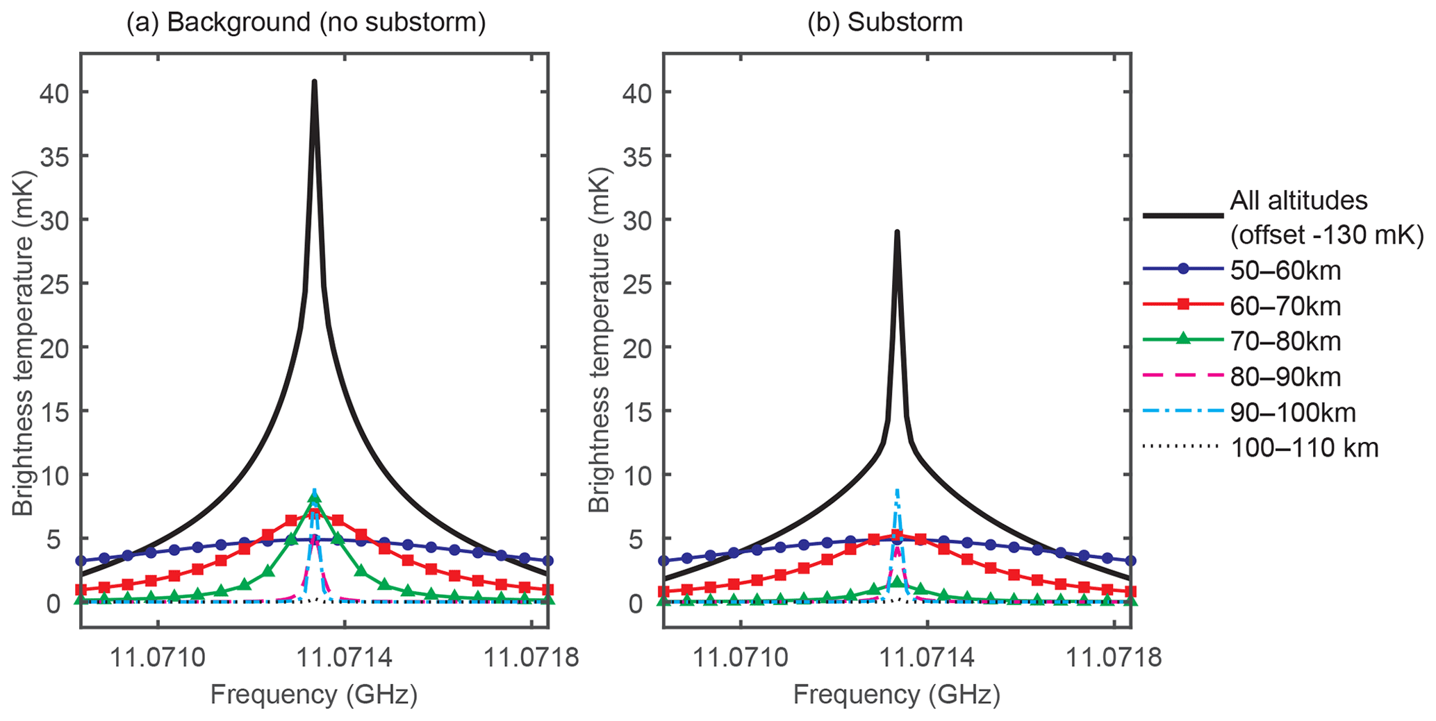
Figure 6Simulated atmospheric spectra for the ozone (O3) 11.072 GHz emission line in clear-sky December conditions using a ground-based radiometer with 10 kHz frequency resolution, 82∘ zenith angle, and 0∘ azimuthal angle located at Kilpisjärvi (69∘03′ N, 20∘48′ E), Finland. Black solid curves show the overall OH emission from all altitudes. Coloured lines show the contributions from 10 km altitude intervals in the range 50–110 km. Panels (a) and (b) show the spectra for background (no substorm) and substorm conditions respectively.
Forward model simulations of the O3 11.072 GHz emission line are shown in Fig. 6a and b, for the substorm and background (no substorm) cases respectively. The solid black lines in each plot are the brightness temperature spectra that would be observed at the ground in clear-sky conditions at a zenith angle of 82∘. The other lines show the contributions to the total signal from 10 km layers in the mesosphere and lower thermosphere between 50 and 110 km. For the substorm scenario, O3 emission is reduced around the peak at 11.072 GHz compared to the background case. The largest decrease in signal corresponds to altitudes 70–80 km, where the modelled reduction in O3 number density during substorms is greatest, with smaller decreases at 60–70 and 80–90 km.

Figure 7Simulated atmospheric spectra for the hydroxyl (OH) 13.441 GHz emission line in clear-sky December conditions using a ground-based radiometer with 10 kHz frequency resolution, 82∘ zenith angle, and 0∘ azimuthal angle located at Kilpisjärvi (69∘03′ N, 20∘48′ E), Finland. Contributions from other atmospheric species have been removed to show changes in the brightness temperature spectra due to OH. Black solid curves show the overall OH emission from all altitudes. Coloured lines show the contributions from 10 km altitude intervals in the range 50–100 km. Panels (a) and (b) are for all sensor polarisations in background (no substorm) and substorm conditions respectively. Similarly, (c) and (d) are for vertical sensor polarisation and (e) and (f) are for horizontal sensor polarisation.
Forward model simulations of the OH 13.441 GHz emission line are shown in Fig. 7a–f. Figure 7a, c, and e are the substorm spectra for three different sensor polarisations: both polarisations, vertical, and horizontal respectively. Figure 7b, d, and f show the corresponding spectra for the background (no substorm) case. The solid black lines in each plot are the brightness temperature spectra that would be observed at the ground in clear-sky conditions at a zenith angle of 82∘. The other lines are the contribution to the total signal from 10 km layers in the mesosphere and lower thermosphere between 50 and 100 km. At an azimuthal angle of 0∘ the vertical polarisation signal is dominated by a single line centred at 13.441 GHz whereas in horizontal polarisation the pair of Zeeman split lines are clearly resolved. For the substorm scenario, OH emission increases around the peak positions compared to the background case. As for O3, the largest changes in signal correspond to altitudes of 70–80 km, where the modelled increase in OH number density during substorms is greatest, with smaller increases at 80–90 km.
3.2 Ozone retrievals
Example retrieval results are shown in Figs. 8 and 9 for simulated clear-sky 6 h observations of the O3 11.072 GHz line at an 82∘ zenith angle from Kilpisjärvi in December substorm and background conditions using a radiometer providing 10 kHz frequency resolution. Figure 8a and e show the final retrieval fits, for the substorm and background cases respectively, which agree with the simulated atmospheric spectra to within the rms baseline noise level. Figure 8c and g compare the true and a priori O3 VMR profiles with the retrieved profiles for the substorm and background cases respectively. The red solid lines and red shaded areas show the average and standard deviations of the retrieved profiles from 500 repeat MC runs with the O3 and H2O profiles used to calculate the spectra, shown by the blue dashed lines, kept constant at the true model values. For both the substorm and background cases the retrieved O3 profiles converge close to the true profiles over the altitudes where information is obtained from the observations, shown by the thicker solid lines and grey shaded areas. The description of how the retrieval altitude range is determined is given in the next paragraph. The differences between the retrieved and true VMR profiles, shown in Fig. 8d and h, are in the range −1.0 to 0.9 ppmv. Above and below the retrieval range the O3 profiles tend towards the a priori values.
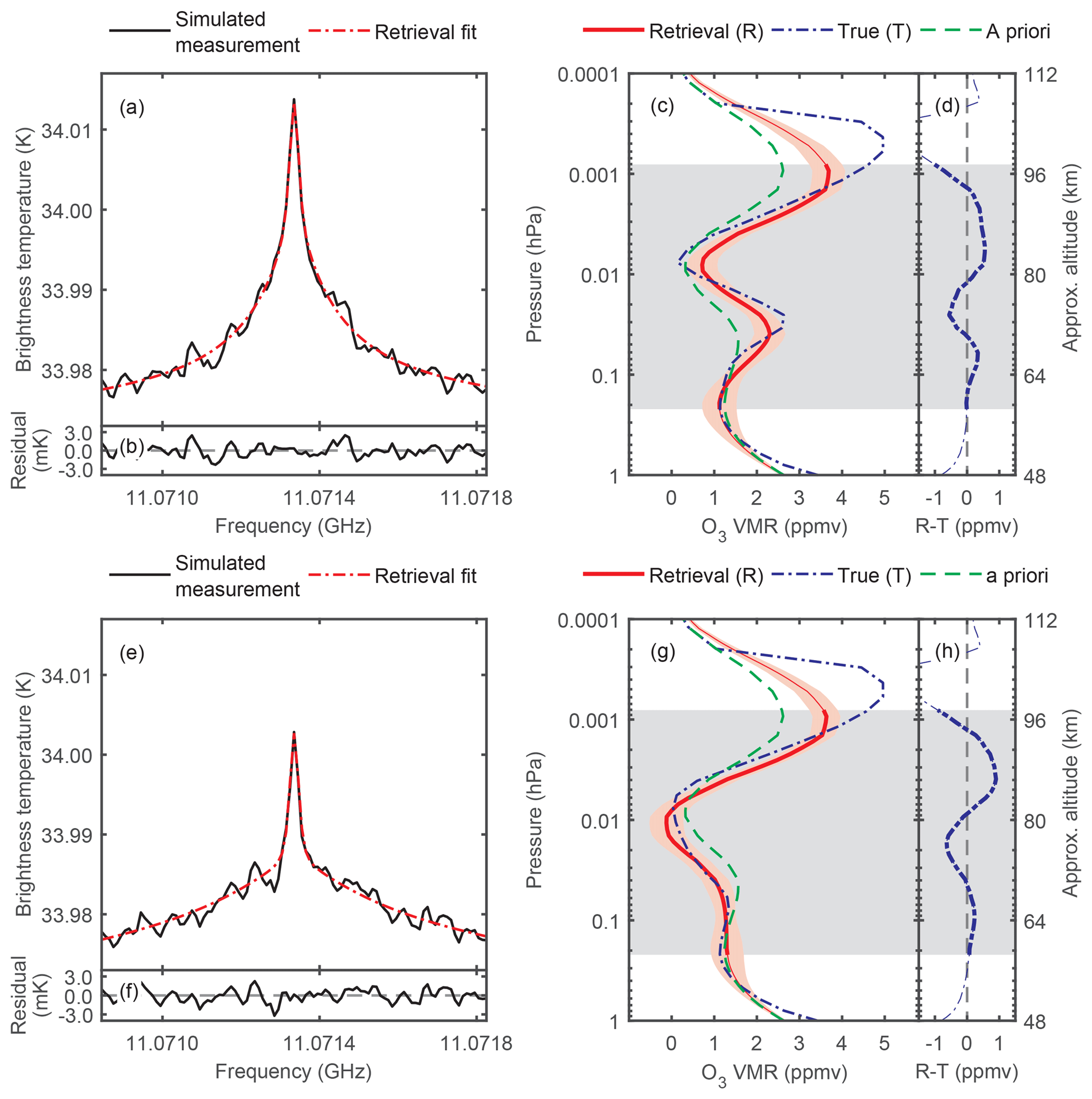
Figure 8Ozone (O3) retrievals for simulated 6 h observations of the O3 11.072 GHz emission line in clear-sky December conditions using a ground-based radiometer at Kilpisjärvi (69∘03′ N, 20∘48′ E), Finland. The forward model clear-sky spectra are calculated using the model O3 profiles for December 2007 with 1 mK baseline noise, 10 kHz frequency resolution, and an 82∘ zenith angle. Panels (a)–(d) show the results using background (no substorm) O3 in the simulations, and (e)–(g) show the results for substorm O3. The simulated O3 spectra and retrieval fits are shown in (a) and (e), and the residual differences are shown in (b) and (f). The a priori, true, and retrieved O3 volume mixing ratio profiles, and the differences between the retrieved and true profiles, are shown in (c)–(d) and (g)–(h) for the background and substorm cases respectively.
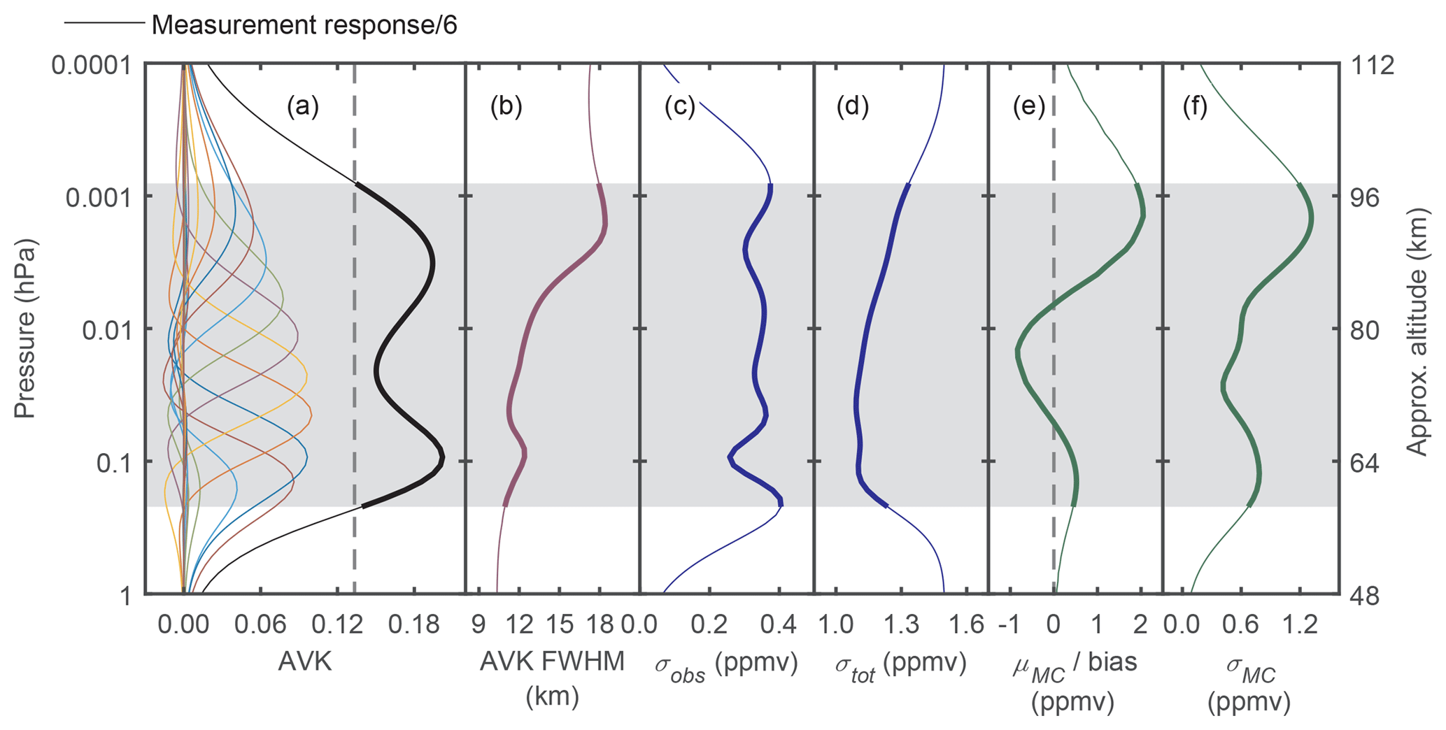
Figure 9Ozone (O3) retrieval diagnostics for simulated 6 h observations of the O3 11.072 GHz emission line using a ground-based radiometer with 1 mK baseline noise level, 10 kHz frequency resolution, and an 82∘ zenith angle located at Kilpisjärvi (69∘03′ N, 20∘48′ E), Finland, in clear-sky December conditions. In (a) every sixth averaging kernel and the scaled measurement response (MR) are shown. Panel (b) shows the full-width half maxima of each averaging kernel (AVK FWHM). The measurement uncertainty (σobs) and total uncertainty (σtot) are shown in (c) and (d) respectively. The mean (μMC) and standard deviation (σMC) of the differences between the retrieved and true profiles from Monte Carlo (MC) error analysis using 500 repeat inversions are shown in (e) and (f) respectively. The vertical grey dashed line in (a) shows the cut-off for MR ≥ 0.8. The grey shaded regions and the thicker sections of the plotted curves indicate the pressure and altitude ranges where MR ≥ 0.8.
The averaging kernels (AVKs) for every sixth retrieved altitude are shown in Fig. 9a. The AVKs describe the relationship among the true, a priori, and retrieved atmospheric states (Rodgers, 2000). None of the AVKs peak at pressure levels above 0.0013 hPa (∼94 km) due to Doppler broadening dominating over pressure broadening. The lowest AVK peaks are at 0.18 hPa (∼60 km). The sum of the AVKs at each altitude, called the measurement (or total) response (MR), represents the extent to which the measurement contributes to the retrieval solution compared to the influence of the a priori at that altitude (Christensen and Eriksson, 2013). The altitude range where the retrieved O3 profile has a high degree of independence from the a priori is identified by MR values higher than 0.8. The retrieval altitude range is –0.22 hPa (∼98–58 km), shown by the thicker sections of the lines and the grey shaded areas in Figs. 8 and 9. Outside of these altitudes (i.e. below 58 and above 98 km) the MR weakens and the O3 values in these regions should be interpreted with caution as the information from the a priori becomes important. The AVKs indicate the range of altitudes over which O3 is observed. In the ideal case the AVKs would be delta functions but in practice they are peaked functions with finite widths dependent on the spatial resolution of the observing system. The FWHM widths of the kernels provide a measure of the vertical resolution of the retrieved profile. The FWHM values shown in Fig. 9b indicate altitude resolutions decreasing from 10.9 km in the lower mesosphere to 18.4 km in the upper mesosphere and lower thermosphere, at altitudes below 98 km. The altitude resolution can also be estimated from the degrees of freedom for signal (DOFS) for the inversion, given by the trace of the AVK matrix (Rodgers, 2000; Ryan et al., 2016). Dividing the retrieved altitude range (∼30 km) by the DOFS over the same range (∼3.2) gives an altitude resolution of 12.0 km, similar to that obtained from the AVK FWHM values.
The OEM calculations provide observation errors (σobs) and total retrieval (observation plus smoothing) errors (σtot), which provide further diagnostic uncertainty estimates of the retrieved profiles. The observation errors describe how the retrieved profiles are affected by measurement noise and are shown in Fig. 9c, with typical values of about 0.34 ppmv. The observation errors are small outside of the range of the AVK peaks as the retrieval tends to the a priori values in these regions and the contribution from the measurement is small. The total retrieval errors shown in Fig. 9d are in the range 1.09–1.34 ppmv and tend towards the smaller a priori standard deviations outside the range of AVK peaks.
The results of the MC error analysis using retrievals from 500 simulated spectra in which O3 and H2O profiles were randomly scaled using a uniform distribution over the range 0.5–2.0, to test the retrieval algorithm's ability to reproduce the true state of the atmosphere, are shown in Fig. 9e–f. Over the trustable altitude range the mean difference (μMC) between the MC retrieved and true profiles is in the range from −0.8 to 2.0 ppmv. The standard deviation (σMC) of the individual retrievals is an estimator for the uncertainty of the O3 retrieval, and the mean value of 0.8 ppmv is approximately double the mean observation error determined from single retrievals (σobs). Both parameters depend on the signal-to-noise ratio of the input spectrum but σMC may more realistically represent actual observations in which mesospheric O3 profiles and column H2O show large variability.
The Jacobian and gain matrices of the O3 forward model indicate that an instrument with 10 kHz frequency resolution will adequately sample the emission line for altitudes of up to ∼98 km where the O3 measurement contributes significantly to the retrieval. The values of the Jacobian, normalised by the layer thickness of the retrieval grid for observations at an 82∘ zenith angle are shown in Fig. 10. Typical values of the Jacobian are ∼0.5 mK (ppmv)−1 km−1 at mesospheric altitudes of 60–90 km where substorms are predicted to have the largest effect on O3 abundance. The effect of predicted O3 changes of ∼1 ppmv over altitudes of 68–86 km on the measured atmospheric brightness temperature will therefore be small, of the order of 9 mK close to the emission line centre, but readily measurable with a baseline noise of 1 mK for a 6 h integration.
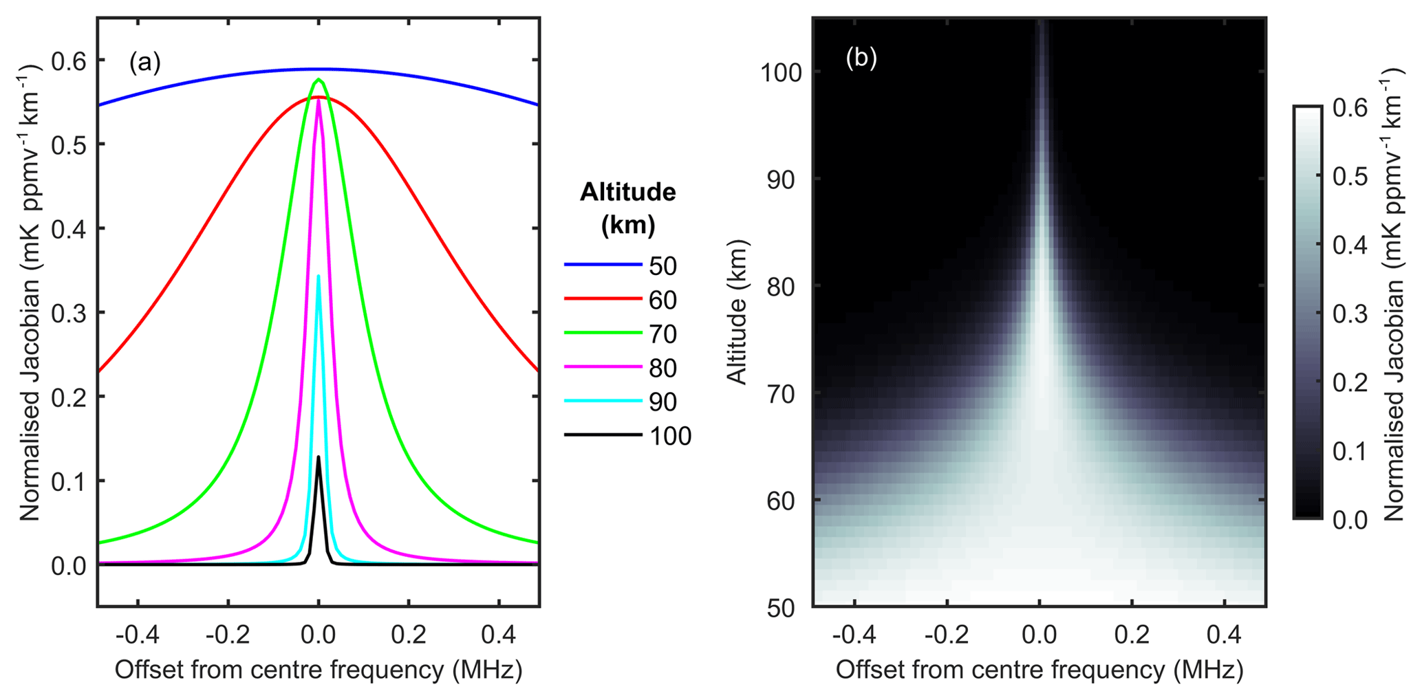
Figure 10Rows of the Jacobian describing the ozone (O3) retrieval, normalised by the layer thickness of the retrieval grid. The data are for retrievals from simulated 6 h observations of the O3 11.072 GHz emission line using a ground-based radiometer with 1 mK baseline noise level, 10 kHz frequency resolution, and an 82∘ zenith angle located at Kilpisjärvi (69∘03′ N, 20∘48′ E), Finland, in clear-sky December conditions. Rows of the Jacobian matrix for selected altitude levels are plotted in (a). The grey scale in (b) indicates the values of the Jacobian matrix.
3.3 Hydroxyl (OH) retrievals
Example retrieval results are shown in Figs. 11 and 12 for simulated clear-sky 6 h observations of the OH 13.441 GHz line at an 82∘ zenith angle and 0∘ azimuthal angle from Kilpisjärvi in December substorm conditions using a radiometer providing 10 kHz frequency resolution with vertical sensor polarisation. Similar results were obtained for retrievals with simulated spectra using sensors measuring horizontal or both polarisations, and with non-zero azimuthal angles. Figure 11a and b show the final retrieval fits which agree with the simulated atmospheric spectra to within the rms baseline noise level. Figure 11c and d compare the true substorm and a priori OH VMR profiles with the retrieved profiles. The red solid lines and red shaded areas show the average and standard deviation of the retrieved profiles from 500 repeat MC runs with the OH and H2O profiles used to calculate the spectra, shown by the dashed blue lines, kept constant at the true model values. The retrieved OH profile approaches the true profiles over the altitudes where information is obtained from the observations, shown by the thicker solid lines and grey shaded areas. However, Fig. 11d shows significant differences, in the range from −13.6 to 3.3 ppbv, between the retrieved and true VMR profiles at altitudes which overlap the OH enhancements. Convolving the true OH profile with the averaging kernels, to account for the limited retrieval resolution, results in much better agreement with differences () in the range from −1.4 to 2.9 ppbv. Above and below the retrieval range the OH profiles approach the a priori OH VMR values, which are close to zero.

Figure 11Hydroxyl (OH) retrievals for simulated 6 h observations of the OH 13.441 GHz emission line using a ground-based radiometer with vertical sensor polarisation at Kilpisjärvi (69∘03′ N, 20∘48′ E), Finland. The forward model clear-sky spectrum is calculated using the model OH profile for substorm conditions in December 2007 with 1 mK baseline noise, 10 kHz frequency resolution, 82∘ zenith angle, and 0∘ azimuthal angle (i.e. north-pointing). The simulated OH spectra and retrieval fit are shown in (a), and the residual differences are shown in (b). The a priori, true, and retrieved OH volume mixing ratio profiles, and the differences between the retrieved and true profiles, are shown in (c) and (d). Note that the scales differ for the upper and lower axes of (d).
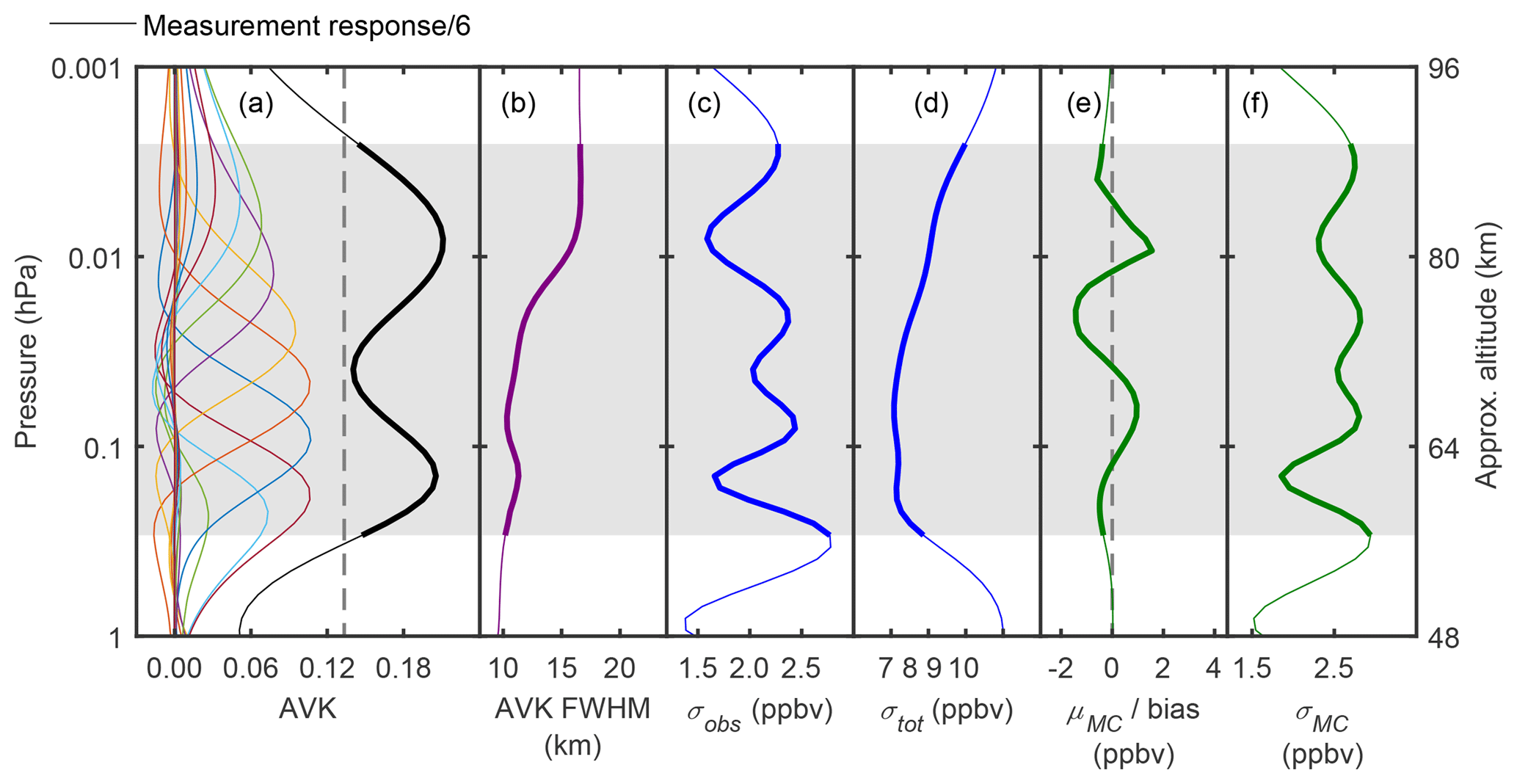
Figure 12Hydroxyl (OH) retrieval diagnostics for simulated 6 h observations of the OH 13.441 GHz emission line using a ground-based radiometer with vertical polarisation, 1 mK baseline noise level, 10 kHz frequency resolution, 82∘ zenith angle, and 0∘ azimuthal angle (i.e. north-pointing) located at Kilpisjärvi (69∘03′ N, 20∘48′ E), Finland, in clear-sky December conditions. In (a) every sixth averaging kernel and the scaled measurement response (MR) are shown. Panel (b) shows the full-width half maxima of each averaging kernel (AVK FWHM). The measurement uncertainty (σobs) and total uncertainty (σtot) are shown in (c) and (d) respectively. The mean (μMC) and standard deviation (σMC) of the differences between the retrieved and true profiles from Monte Carlo (MC) error analysis using 500 repeat inversions are shown in (e) and (f) respectively. The vertical grey dashed line in (a) shows the cut-off for MR ≥ 0.8. The grey shaded regions and the thicker sections of the plotted curves indicate the pressure and altitude ranges where MR ≥ 0.8.
The AVKs for every sixth retrieved altitude are shown in Fig. 12a. None of the AVKs peak at pressure levels above 0.003 hPa (∼88 km) due to Doppler broadening dominating over pressure broadening. The lowest AVK peaks at 0.24 hPa (∼58 km). The estimated retrieval range, where the MR is larger than 0.8, is –0.29 hPa (∼90–56 km), shown by the thicker sections of the lines and the grey shaded areas in Figs. 11 and 12. Outside of these altitudes (i.e. below 56 and above 90 km) the MR weakens and the OH values in these regions should be interpreted with caution as the information from the a priori becomes important. The AVK FWHM values shown in Fig. 12b indicate altitude resolutions decreasing from 10.2 km in the lower mesosphere to 16.6 km in the upper mesosphere, at altitudes below 90 km. Dividing the retrieved altitude range (∼34 km) by the DOFS over the same range (∼3.0) gives an estimated altitude resolution of 11.0 km, similar to that obtained from the AVK FWHM values. The observation errors (σobs) shown in Fig. 12c have typical values of 2.1 ppbv and are smaller outside of the range of the AVK peaks as the retrieval tends to the a priori values in these regions and the contribution from the measurement is small. The total retrieval errors (σtot) shown in Fig. 12d are in the range 7.1–9.0 ppbv and tend towards the larger a priori standard deviations when they are outside the range of AVK peaks.
The results of the MC error analysis using retrievals from 500 simulated spectra in which OH and H2O profiles were randomly scaled by 0.5–2.0 are shown in Fig. 12e–f. Over the trustable altitude range the mean difference (μMC) between the MC retrieved and true profiles is in the range from −1.4 to 1.6 ppbv. The standard deviation (σMC) of the individual retrievals is an estimator for the uncertainty of the OH retrieval, and the mean value of 2.6 ppbv is similar the mean observation error determined from single retrievals (σobs). Both parameters depend on the signal-to-noise ratio of the input spectrum but σMC may more realistically represent actual observations in which mesospheric OH profiles and column H2O show large variability.
The Jacobian and gain matrices of the OH vertical polarisation forward model indicate that, as for O3, the OH emission line should be adequately sampled by an instrument with 10 kHz frequency resolution for all altitudes where the OH measurement contributes significantly to the retrieval. The values of the Jacobian, normalised by the layer thickness of the retrieval grid for observations at an 82∘ zenith angle, are shown in Fig. 13. Typical values of the Jacobian are ∼0.09 mK (ppbv)−1 km−1 at mesospheric altitudes of 60–90 km where substorms are predicted to have the largest effect on OH abundance. The predicted changes in OH VMR, by up to ∼20 ppbv for the altitude range 64–84 km, will have a small effect on the measured atmospheric brightness temperatures, producing a ∼10 mK increase close to the emission line centre. However, the enhanced OH microwave signal during substorm activity would be measurable with a baseline noise of 1 mK for a 6 h integration.
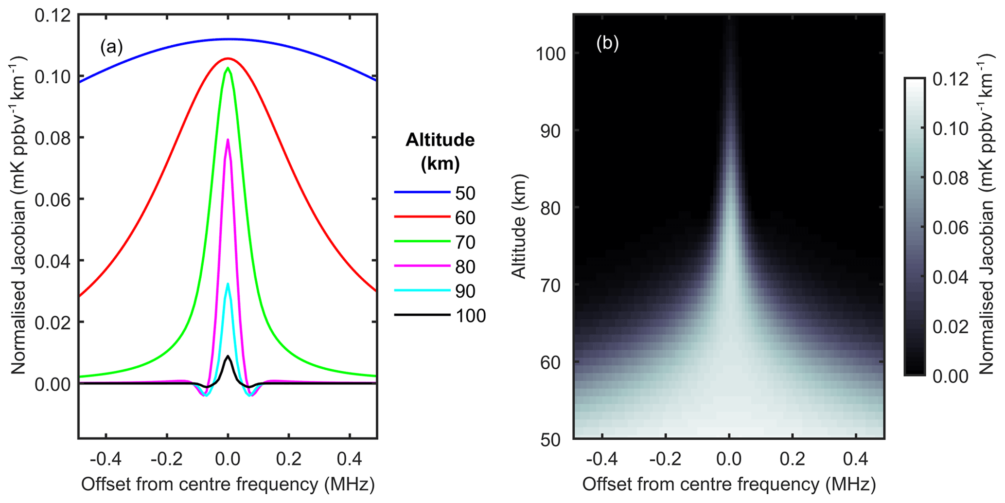
Figure 13Rows of the Jacobian describing the hydroxyl (OH) retrieval, normalised by the layer thickness of the retrieval grid. The data are for retrievals from simulated 6 h observations of the OH 13.441 GHz emission line using a ground-based radiometer with vertical polarisation, 1 mK baseline noise level, 10 kHz frequency resolution, 82∘ zenith angle, and 0∘ azimuthal angle (i.e. north-pointing) located at Kilpisjärvi (69∘03′ N, 20∘48′ E), Finland, in clear-sky December conditions. Rows of the Jacobian matrix for selected altitude levels are plotted in (a). The grey scale in (b) indicates the values of the Jacobian matrix.
The proof-of-concept simulations demonstrate that changes in O3 and OH abundance in the high-latitude or polar middle and upper atmosphere, associated with geomagnetic substorm and other EEP processes, could be profiled using ground-based passive microwave measurements in the Ku-band 11–14 GHz region and OEM retrieval. At these frequencies tropospheric attenuation is small and mesospheric emission signals are transmitted to the ground with low loss. Comparable high atmospheric transmittances are calculated for various high-latitude NH and Antarctic sites in winter and summer, suggesting that different meteorology and location should have little impact on the proposed O3 and OH observations.
For a radiometer performing 6 h measurements of the 11.072 GHz O3 emission line with 10 kHz frequency resolution and a rms baseline noise of 1 mK, O3 could be profiled over –0.22 hPa (∼98–58 km) with 11–18 km height resolution (∼12 km from DOFS analysis) and ∼1 ppmv uncertainty. For the equivalent OH 13.441 GHz measurement, demonstrated for vertical sensor polarisation, OH could be profiled over –0.29 hPa (∼90–56 km), also with 10–17 km height resolution (∼11 km from DOFS analysis) and ∼3 ppbv uncertainty. Such observations would allow the diurnal variations in mesospheric O3 and OH to be characterised when abundances are relatively high, e.g. during night-time and polar winter. Measurement times of 24 h or longer would be necessary with less sensitive receivers or for measuring lower abundances. However, these measurements would still provide valuable data, in particular for the secondary ozone layer above 90 km as satellite measurements of this region become increasingly sparse. We have used simulations of atmospheric spectra from Kilpisjärvi, Finland, as a test case to assess the feasibility of such measurements but demonstrate that similar results would be achieved by instruments deployed at other high-latitude NH sites and in Antarctica.
LNB receivers operating at the Ku-band emission frequencies of O3 and OH are commercially available. LNBs covering the O3 frequency (11.072 GHz) have a noise factor typically in the range 0.7–1.3 dB, although suppliers specify values as low as 0.1 dB. For coverage of the OH emission line frequency (13.441 GHz) the stated LNB noise factor is ∼1.2 dB. However, measurements reported by Tenneti and Rogers (2009) suggest that inexpensive satellite TV downconverters can achieve a noise factor as low as ∼0.23 dB. If this high level of LNB performance is confirmed, a single receiver operating at room temperature would achieve 6 h O3 spectrum measurements with the required rms baseline noise level of 1 mK. Otherwise, for the proposed O3 and OH observations, either simultaneous measurements by an array of multiple receivers or using single receivers cooled to ∼168 K for O3 and ∼46 K for OH would be needed. Monitoring of O3 in the same volume of the atmosphere using three LNB receivers mounted in front of a “Direct TV” offset parabolic dish has been reported (Rogers et al., 2012). With six spectrometers simultaneously measuring both polarisations from each of the three receivers, in the ideal case the improvement in signal-to-noise ratio compared to a single radiometer is , although non-optimum matching of the LNB beam profiles and antenna focus would impact the performance. Scaling up to 24 independent spectrometers for the O3 measurements would be relatively straightforward using 12 receivers each measuring both polarisations, mounted singly or with two or three LNBs bundled together at each antenna focus point. Atmospheric observations recorded by each spectrometer could then be combined to achieve a improvement in signal-to-noise ratio. For OH, the greater complexity and cost of constructing 80 independent spectrometers operating at 13.441 GHz could make use of a single low-temperature receiver the better option. For low-temperature operation, liquid nitrogen-cooled cryostats readily attain ∼90 K, meeting the requirements for O3 observations. However, this cooling method requires a supply of liquid nitrogen into either a continuous flow or reservoir design of cryostat. Alternatively, LNBs mounted on the cold-head of a Gifford–McMahon closed-cycle helium cryocooler (e.g. Radebaugh, 2009; de Waele, 2011) could be operated continuously at temperatures in the range 4–77 K.
The next steps towards developing suitable instruments include selecting and testing commercially available LNB receiver and antenna components and verifying the optimum configuration for making the proposed mesospheric O3 and OH observations. If tests confirm that low-cost satellite TV components can reliably achieve the desired performance (e.g. LNBs with a noise factor of 0.23 dB or lower) then the increased complexity and cost of designing and building a system using numerous multiple receivers or cryogenic cooling would be avoided, for O3 11.072 GHz measurements at least. It should be noted that other natural and artificial sources may produce signals at frequencies that overlap the O3 and OH microwave emissions. Potential interference from such sources may be mitigated by observing at remote high-latitude locations and by carefully pointing the receiver antenna to minimise directional pickup of spurious signals in the instrument field of view. OH microwave line Zeeman splitting needs to be adequately modelled in the retrieval algorithm, and the spectroscopic parameters need to be verified and optimised. Furthermore, during geomagnetic storms, rapid, localised fluctuations in the Earth's magnetic field can occur, which may not be well reproduced by a priori data from models such as IGRF. Instead, a better approach may be to use magnetometer data provided by nearby geophysical observatories to constrain the OH retrievals, or to allow the retrieval to adjust the magnetic field from a priori values to give an optimum fit to the observed line shape.
The model and simulation datasets used in this study are available from the UK Polar Data Centre (https://doi.org/10.5285/57858a9a-d814-412c-8e79-9a542cd055d4; Newnham et al., 2018b).
DAN performed the ozone and hydroxyl microwave spectrum and retrieval simulations, and co-ordinated the study. AS and PTV carried out atmospheric model calculations and provided model data inputs for the simulation study. MAC and MK provided technical data on the configuration and performance of existing 11.072 GHz ozone spectrometers. All authors discussed the results and commented on the paper.
The authors declare that they have no conflict of interest.
This work has been supported in part by the UK's Natural Environment Research
Council (NERC) Technologies Proof-of-Concept grant reference NE/P003478/1
“Satellite TV-based Ozone and OH Observations using Radiometric Measurements
(STO3RM)” awarded to David A. Newnham. The work of Pekka T. Verronen
was supported by the Academy of Finland (project 276926 – SECTIC: Sun-Earth
Connection Through Ion Chemistry). The authors thank the ARTS and Qpack
development teams and Peter Kirsch at BAS for assistance configuring and
running the code, Monika E. Andersson (FMI) for providing WACCM-D datasets,
and Alan E. E. Rogers at the Massachusetts Institute of Technology (MIT)
Haystack Observatory for helpful discussions. Aaron Hendry is acknowledged
for providing computer code (GEO2CGM) to facilitate the conversion from
spherical geographic coordinates to spherical corrected geomagnetic
coordinates.
Edited by: Gabriele
Stiller
Reviewed by: three anonymous referees
Andersson, M. E., Verronen, P. T., Rodger, C. J., Clilverd, M. A., and Seppälä, A.: Missing driver in the Sun–Earth connection from energetic electron precipitation impacts mesospheric ozone, Nat. Commun., 5, 5197, https://doi.org/10.1038/ncomms6197, 2014a.
Andersson, M. E., Verronen, P. T., Rodger, C. J., Clilverd, M. A., and Wang, S.: Longitudinal hotspots in the mesospheric OH variations due to energetic electron precipitation, Atmos. Chem. Phys., 14, 1095–1105, https://doi.org/10.5194/acp-14-1095-2014, 2014b.
Arsenovic, P., Rozanov, E., Stenke, A., Funke, B., Wissing, J. M., Mursula, K., Tummon, F., and Peter, T.: The influence of middle range energy electrons on atmospheric chemistry and regional climate, J. Atmos. Sol.-Terr. Phy., 149, 180–190, https://doi.org/10.1016/j.jastp.2016.04.008, 2016.
Baumgaertner, A. J. G., Seppälä, A., Jöckel, P., and Clilverd, M. A.: Geomagnetic activity related NOx enhancements and polar surface air temperature variability in a chemistry climate model: modulation of the NAM index, Atmos. Chem. Phys., 11, 4521–4531, https://doi.org/10.5194/acp-11-4521-2011, 2011.
Brasseur, G. P. and Solomon, S.: Aeronomy of the Middle Atmosphere, 3rd Edn., Springer, Dordrecht, the Netherlands, 2005.
Brinksma, E. J., Meijer, Y. J., McDermid, I. S., Cageao, R. P., Bergwerff, J. B., Swart, D. P. J., Ubachs, W., Matthews, W. A., Hogervorst, W., and Hovenier, J. W.: First lidar observations of mesospheric hydroxyl, Geophys. Res. Lett., 25, 51–54, https://doi.org/10.1029/97GL53561, 1998a.
Brinksma, E. J., Meijer, Y. J., McDermid, I. S., Cageao, R. P., Bergwerff, J. B., Swart, D. P. J., Ubachs, W., Matthews, W. A., Hogervorst, W., and Hovenier, J. W.: Correction to “First lidar observations of mesospheric hydroxyl”, Geophys. Res. Lett., 25, 521, https://doi.org/10.1029/98GL00119, 1998b.
Buehler, S. A., Eriksson, P., Kuhn, T., von Engeln, A., and Verdes, C.: ARTS, the atmospheric radiative transfer simulator, J. Quant. Spectrosc. Ra., 91, 65–93, https://doi.org/10.1016/j.jqsrt.2004.05.051, 2005.
Buehler, S. A., Mendrok, J., Eriksson, P., Perrin, A., Larsson, R., and Lemke, O.: ARTS, the Atmospheric Radiative Transfer Simulator – version 2.2, the planetary toolbox edition, Geosci. Model Dev., 11, 1537–1556, https://doi.org/10.5194/gmd-11-1537-2018, 2018.
Christensen, O. M. and Eriksson, P.: Time series inversion of spectra from ground-based radiometers, Atmos. Meas. Tech., 6, 1597–1609, https://doi.org/10.5194/amt-6-1597-2013, 2013.
Clancy, R. T., Sandor, B. J., Rusch, D. W., and Muhleman, D. O.: Microwave observations and modeling of O3, H2O, and HO2 in the mesosphere, J. Geophys. Res., 99, 5465–5473, https://doi.org/10.1029/93JD03471, 1994.
Clough, S., Shephard, M., Mlawer, E., Delamere, J., Iacono, M., Cady-Pereira, K., Boukabara, S., and Brown, P.: Atmospheric radiative transfer modeling: a summary of the AER codes, J. Quant. Spectrosc. Ra., 91, 233–244, 2005.
Cresswell-Moorcock, K., Rodger, C. J., Kero, A., Collier, A. B., Clilverd, M. A., Häggström, I., and Pitkänen, T.: A reexamination of latitudinal limits of substorm-produced energetic electron precipitation, J. Geophys. Res.-Space, 118, 6694–6705, https://doi.org/10.1002/jgra.50598, 2013.
Daae, M., Straub, C., Espy, P. J., and Newnham, D. A.: Atmospheric ozone above Troll station, Antarctica observed by a ground based microwave radiometer, Earth Syst. Sci. Data, 6, 105–115, https://doi.org/10.5194/essd-6-105-2014, 2014.
de Waele, A. T. A. M.: Basic operation of cryocoolers and related thermal machines, J. Low Temp. Phys., 164, 179, https://doi.org/10.1007/s10909-011-0373-x, 2011.
Englert, C. R., Stevens, M. H., Siskind, D. E., Harlander, J. M., and Roesler, F. L.: Spatial Heterodyne Imager for Mesospheric Radicals on STPSat-1, J. Geophys. Res., 115, D20306, https://doi.org/10.1029/2010JD014398, 2010.
Eriksson, P., Jiménez, C., and Buehler, S. A.: Qpack, a general tool for instrument simulation and retrieval work, J. Quant. Spectrosc. Ra., 91, 47–64, https://doi.org/10.1016/j.jqsrt.2004.05.050, 2005.
Eriksson, P., Buehler, S. A., Davis, C. P., Emde, C., and Lemke, O.: ARTS, the atmospheric radiative transfer simulator, version 2, J. Quant. Spectrosc. Ra., 112, 1551–1558, https://doi.org/10.1016/j.jqsrt.2011.03.001, 2011.
Finlay, C. C., Maus, S., Beggan, C. D., Bondar, T. N., Chambodut, A., Chernova, T. A., Chulliat, A., Golovkov, V. P., Hamilton, B., Hamoudi, M., Holme, R., Hulot, G., Kuang, W., Langlais, B., Lesur, V., Lowes, F. J., Lühr, H., Macmillan, S., Mandea, M., McLean, S., Manoj, C., Menvielle, M., Michaelis, I., Olsen, N., Rauberg, J., Rother, M., Sabaka, T. J., Tangborn, A., Tøffner-Clausen, L., Thébault, E., Thomson, A. W. P., Wardinski, I., Wei, Z., and Zvereva, T. I.: International geomagnetic reference field: The eleventh generation, Geophys. J. Int., 183, 1216–1230, https://doi.org/10.1111/j.1365-246X.2010.04804.x, 2010.
Froidevaux, L., Jiang, Y. B., Lambert, A., Livesey, N. J., Read, W. G., Waters, J. W., Browell, E. V., Hair, J. W., Avery, M. A., McGee, T. J., Twigg, L. W., Sumnicht, G. K., Jucks, K. W., Margitan, J. J., Sen, B., Stachnik, R. A., Toon, G. C., Bernath, P. F., Boone, C. D., Walker, K. A., Filipiak, M. J., Harwood R. S., Fuller, R. A., Manney, G. L., Schwartz, M. J., Daffer, W. H., Drouin, B. J., Cofield, R. E., Cuddy, D. T., Jarnot, R. F., Knosp, B. W., Perun, V. S., Snyder, W. V., Stek, P. C., Thurstans, R. P., and Wagner, P. A.: Validation of Aura Microwave Limb Sounder stratospheric ozone measurements, J. Geophys. Res., 113, D15S20, https://doi.org/10.1029/2007JD008771, 2008.
Gordon, I. E., Rothman, L. S., Hill, C., Kochanov, R. V., Tan, Y., Bernath, P. F., Birk, M., Boudon, V., Campargue, A., Chance, K. V., Drouin, B. J., Flaud, J.-M., Gamache, R. R., Hodges, J. T., Jacquemart, D., Perevalov, V. I., Perrin, A., Shine, K. P., Smith, M.-A. H., Tennyson, J., Toon, G. C., Tran, H., Tyuterev, V. G., Barbe, A., Császár, A. G., Devi, V. M., Furtenbacher, T., Harrison, J. J., Hartmann, J.-M., Jolly, A., Johnson, T. J., Karman, T., Kleiner, I., Kyuberis, A. A., Loos, J., Lyulin, O. M., Massie, S. T., Mikhailenko, S. N., Moazzen-Ahmadi, N., Müller, H. S. P., Naumenko, O. V., Nikitin, A. V., Polyansky, O. L., Rey, M., Rotger, M., Sharpe, S. W., Sung, K., Starikova, E., Tashkun, S. A., Vander Auwera, J., Wagner, G., Wilzewski, J., Wcislo, P., Yu, S., and Zak, E. J.: The HITRAN2016 molecular spectroscopic database, J. Quant. Spectrosc. Ra., 203, 3–69, https://doi.org/10.1016/j.jqsrt.2017.06.038, 2017.
Hartogh, P., Jarchow, C., Sonnemann G. R., and Grygalashvyly, M.: On the spatiotemporal behavior of ozone within the mesosphere/mesopause region during nearly polar night conditions, J. Geophys. Res., 109, D18303, https://doi.org/10.1029/2004JD004576, 2004.
Jackman, C. H. and McPeters, R. D.: The effect of solar proton events on ozone and other constituents, Solar variability and its effects on climate, Geophysical Monograph Series, Vol. 141, 305–319, American Geophysical Union, Washington, DC, https://doi.org/10.1029/141GM21, 2004.
Kraus, J. D.: Radio astronomy, Powell, Ohio, Cygnus-Quasar, 2nd Edn., ISBN 10-1882484002, ISBN 13-9781882484003, 1986.
Kuntz, M.: A new implementation of the Humlicek algorithm for the calculation of the Voigt profile function, J. Quant. Spectrosc. Ra., 57, 819–824, 1997.
Larsson, R., Buehler, S. A., Eriksson P., and Mendrok, J.: A treatment of the Zeeman effect using Stokes formalism and its implementation in the Atmospheric Radiative Transfer Simulator (ARTS), J. Quant. Spectrosc. Ra., 133, 445–453, https://doi.org/10.1016/j.jqsrt.2013.09.006, 2014.
Marsh, D. R., Mills, M. J., Kinnison, D. E., and Lamarque, J.-F.: Climate change from 1850 to 2005 simulated in CESM1 (WACCM), J. Climate, 26, 7372–7391, https://doi.org/10.1175/JCLI-D-12-00558.1, 2013.
Melsheimer, C., Verdes, C., Buehler, S. A., Emde, C., Eriksson, P., Feist, D. G., Ichizawa, S., John, V. O., Kasai, Y., Kopp, G., Koulev, N., Kuhn, T., Lemke, O., Ochiai, S., Schreier, F., Sreerekha, T. R., Suzuki, M., Takahashi, C., Tsujimaru, S., and Urban, J.: Intercomparison of general purpose clear sky atmospheric radiative transfer models for the millimeter/submillimeter spectral range, Radio Sci., 40, RS1007, https://doi.org/10.1029/2004RS003110, 2005.
Minschwaner, K., Manney, G. L., Wang, S. H., and Harwood, R. S.: Hydroxyl in the stratosphere and mesosphere – Part 1: Diurnal variability, Atmos. Chem. Phys., 11, 955-962, https://doi.org/10.5194/acp-11-955-2011, 2011.
Mironova, I. A., Aplin, K. L., Arnold, F., Bazilevskaya, G. A., Harrison, R. G., Krivolutsky, A. A., Nicoll, K. A., Rozanov, E. V., Turunen, E., and Usoskin, I. G.: Energetic particle influence on the Earth's atmosphere, Space Sci. Rev., 194, 1–96, https://doi.org/10.1007/s11214-015-0185-4, 2015.
Mlawer, E. J., Payne, V. H., Moncet, J.-L., Delamere, J. S., Alvarado, M. J., and Tobin, D. C.: Development and recent evaluation of the MT-CKD model of continuum absorption, Philos. T. R. Soc. A, 370, 2520–2556, 2012.
Newnham, D. A., Clilverd, M. A., Rodger, C. J., Hendrickx, K., Megner, L., Kavanagh, A. J., Seppälä, A., Verronen, P. T., Andersson, M. E., Marsh, D. R., Kovács, T., Feng, W., and Plane, J. M. C.: Observations and modeling of increased nitric oxide in the Antarctic polar middle atmosphere associated with geomagnetic storm-driven energetic electron precipitation, J. Geophys. Res.-Space, 123, https://doi.org/10.1029/2018JA025507, 2018a.
Newnham, D., Verronen, P., and Seppälä, A.: Model data for simulating atmospheric microwave spectra at 11.072 GHz and 13.441 GHz and performing retrievals of ozone (O3) and hydroxyl (OH) vertical profiles, Polar Data Centre, Natural Environment Research Council, UK, https://doi.org/10.5285/57858a9a-d814-412c-8e79-9a542cd055d4, 2018b.
Pickett, H. M., Drouin, B. J., Canty, T., Salawitch, R. J., Fuller, R. A., Perun, V. S., Livesey, N. J., Waters, J. W., Stachnik, R. A., Sander, S. P., Traub, W. A., Jucks, K. W., and Minschwaner, K.: Validation of Aura Microwave Limb Sounder OH and HO2 measurements, J. Geophys. Res., 113, D16S30, https://doi.org/10.1029/2007JD008775, 2008.
Radebaugh, R.: Cryocoolers: the state of the art and recent developments, J. Phys.-Condens. Mat., 21, 164219, https://doi.org/10.1088/0953-8984/21/16/164219, 2009.
Radford, H. E.: Microwave Zeeman effect of free hydroxyl radicals, Phys. Rev., 122, 114, https://doi.org/10.1103/PhysRev.122.114, 1961.
Rodger, C. J., Cresswell-Moorcock, K., and Clilverd, M. A.: Nature's Grand Experiment: Linkage between magnetospheric convection and the radiation belts, J. Geophys. Res.-Space, 121, 171–189, https://doi.org/10.1002/2015JA021537, 2016.
Rodgers, C. D.: Inverse methods for atmospheric sounding: Theory and Practice, Vol. 2 of Series on Atmospheric, Ocean and Planetary Physics, World Scientific, https://doi.org/10.1142/3171, 2000.
Rogers, A. E. E., Lekberg, M., and Pratap, P.: Seasonal and diurnal variations of ozone near the mesopause from observations of the 11.072-GHz line, J. Atmos. Ocean. Tech., 26, 2192–2199, https://doi.org/10.1175/2009JTECHA1291.1, 2009.
Rogers, A. E. E., Erickson, P., Fish, V. L., Kittredge, J., Danford, S., Marr, J. M., Arndt, M. B., Sarabia, J., Costa, D., and May, S. K.: Repeatability of the seasonal variations of ozone near the mesopause from observations of the 11.072-GHz line, J. Atmos. Ocean. Tech., 29, 1492–1504, https://doi.org/10.1175/JTECH-D-11-00193.1, 2012.
Ryan, N. J., Walker, K. A., Raffalski, U., Kivi, R., Gross, J., and Manney, G. L.: Ozone profiles above Kiruna from two ground-based radiometers, Atmos. Meas. Tech., 9, 4503–4519, https://doi.org/10.5194/amt-9-4503-2016, 2016.
Sastry, K. V. L. N. and Vanderlinde, J.: Low-field Zeeman effect of OH in the 2Π3∕2, , 9/2, 11/2, 13/2, and 15/2 states, J. Mol. Spectrosc., 83, 332–338, https://doi.org/10.1016/0022-2852(80)90057-0, 1980.
Semeniuk, K., Fomichev, V. I., McConnell, J. C., Fu, C., Melo, S. M. L., and Usoskin, I. G.: Middle atmosphere response to the solar cycle in irradiance and ionizing particle precipitation, Atmos. Chem. Phys., 11, 5045–5077, https://doi.org/10.5194/acp-11-5045-2011, 2011.
Seppälä, A., Randall, C. E., Clilverd, M. A., Rozanov, E., and Rodger, C. J.: Geomagnetic activity and polar surface air temperature variability, J. Geophys. Res.-Space, 114, A10312, https://doi.org/10.1029/2008JA014029, 2009.
Seppälä, A., Lu, H., Clilverd, M. A., and Rodger, C. J.: Geomagnetic activity signatures in wintertime stratosphere wind, temperature, and wave response, J. Geophys. Res.-Atmos., 118, 2169–2183, https://doi.org/10.1002/jgrd.50236, 2013.
Seppälä, A., Clilverd, M. A., Beharrell, M. J., Rodger, C. J., Verronen, P. T., Andersson, M. E., and Newnham, D. A.: Substorm-induced energetic electron precipitation: Impact on atmospheric chemistry, Geophys. Res. Lett., 42, 8172–8176, https://doi.org/10.1002/2015GL065523, 2015.
Sinnhuber, M., Nieder, H., and Wieters, N.: Energetic particle precipitation and the chemistry of the mesosphere/lower thermosphere, Surv. Geophys., 33, 1281–1334, https://doi.org/10.1007/s10712-012-9201-3, 2012.
Siskind, D. E., Stevens, M. H., Englert, C. R., and Mlynczak, M. G.: Comparison of a photochemical model with observations of mesospheric hydroxyl and ozone, J. Geophys. Res., 118, 195–207, https://doi.org/10.1029/2012JD017971, 2013.
Smith, A. K., Harvey, V. L., Mlynczak, M. G., Funke, B., García-Comas, M., Hervig, M., Kaufmann, M., Kyrölä, E., López-Puertas, M., McDade, I., Randall, C. E., Russell III, J. M., Sheese, P. E., Shiotani, M., Skinner, W. R., Suzuki, M., and Walker, K. A.: Satellite observations of ozone in the upper mesosphere, J. Geophys. Res.-Atmos., 118, 5803–5821, https://doi.org/10.1002/jgrd.50445, 2013.
Smith, S. M., Baumgardner, J., Mertens, C. J., Russell, J. M., Mlynczak, M. G., and Mendillo, M.: Mesospheric OH temperatures: Simultaneous ground-based and SABER OH measurements over Millstone Hill, Adv. Space Res., 45, 239–246, https://doi.org/10.1016/j.asr.2009.09.022, 2010.
Summers, M. E., Conway, R. R., Siskind, D. E., Stevens, M. H., Offermann, D., Riese, M., Preusse, P., Strobel, D. F., and Russell III, J. M.: Implications of satellite OH observations for middle atmospheric H2O and ozone, Science, 277, 1967–1969, 1997.
Tenneti, S. N. and Rogers, A. E. E.: Development of an optimized antenna and other enhancements of a spectrometer for the study of ozone in the mesosphere, VSRT and MOSAIC Memo 063, available at: https://www.haystack.mit.edu/edu/undergrad/VSRT/VSRT_Memos/063.pdf (last access: 21 February 2019), 2009.
Thébault, E., Finlay, C. C., Beggan, C. D., Alken, P., Aubert, J., Barrois, O., Bertrand, F., Bondar, T., Boness, A., Brocco, L., Canet, E., Chambodut, A., Chulliat, A., Coïsson, P., Civet, F., Du, A., Fournier, A., Fratter, I., Gillet, N., Hamilton, B., Hamoudi, M., Hulot, G., Jager, T., Korte, M., Kuang, W., Lalanne, X., Langlais, B., Léger, J.-M., Lesur, V., Lowes, F. J., Macmillan, S., Mandea, M., Manoj, C., Maus, S., Olsen, N., Petrov, V., Ridley, V., Rother, M., Sabaka, T. J., Saturnino, D., Schachtschneider, R., Sirol, O., Tangborn, A., Thomson, A., Tøffner-Clausen, L., Vigneron, P., Wardinski, I., and Zvereva, T.: International Geomagnetic Reference Field: the 12th generation, Earth Planets Space, 67, 79, https://doi.org/10.1186/s40623-015-0228-9, 2015.
Turunen, E., Verronen, P. T., Seppälä, A., Rodger, C. J., Clilverd, M. A., Tamminen, J., Enell, C.-F., and Ulich, T.: Impact of different energies of precipitating particles on NOx generation in the middle and upper atmosphere during geomagnetic storms, J. Atmos. Sol.-Terr. Phy., 71, 1176–1189, https://doi.org/10.1016/j.jastp.2008.07.005, 2009.
Van Vleck, J. and Huber, D.: Absorption, emission, and line-breadths: A semi-historical perspective, Rev. Mod. Phys., 49, 939, https://doi.org/10.1103/RevModPhys.49.939, 1977.
Verronen, P. T. and Lehmann, R.: Analysis and parameterisation of ionic reactions affecting middle atmospheric HOx and NOy during solar proton events, Ann. Geophys., 31, 909–956, https://doi.org/10.5194/angeo-31-909-2013, 2013.
Verronen, P. T. and Lehmann, R.: Enhancement of odd nitrogen modifies mesospheric ozone chemistry during polar winter, Geophys. Res. Lett., 42, 10445–10452, https://doi.org/10.1002/2015GL066703, 2015.
Verronen, P. T., Seppälä, A., Clilverd, M. A., Rodger, C. J., Kyrölä, E., Enell, C.-F., Ulich, T., and Turunen, E.: Diurnal variation of ozone depletion during the October–November 2003 solar proton events, J. Geophys. Res., 110, A09S32, https://doi.org/10.1029/2004JA010932, 2005.
Verronen, P. T., Rodger, C. J., Clilverd, M. A., and Wang, S.: First evidence of mesospheric hydroxyl response to electron precipitation from the radiation belts, J. Geophys. Res., 116, D07307, https://doi.org/10.1029/2010JD014965, 2011.
Verronen, P. T., Andersson, M. E., Marsh, D. R., Kovács, T., and Plane, J. M. C.: WACCM-D – Whole Atmosphere Community Climate Model with D-region ion chemistry, J. Adv. Model. Earth Sy., 8, 954–975, https://doi.org/10.1002/2015MS000592, 2016.
von Zahn, U., Fricke, K. H., Gerndt, R., and Blix, T.: Mesospheric temperatures and the OH layer height as derived from ground-based lidar and OH* spectrometry, J. Atmos. Terr. Phys., 49, 863–869, https://doi.org/10.1016/0021-9169(87)90025-0, 1987.
Yee, J.-H., Crowley, G., Roble, R. G., Skinner, W. R., Burrage, M. D., and Hays, P. B.: Global simulations and observations of O(1S), O2(1Σ) and OH mesospheric nightglow emissions, J. Geophys. Res., 102, 19949–19968, https://doi.org/10.1029/96JA01833, 1997.
Zawedde, A. E., NesseTyssøy, H., Stadsnes, J., and Sandanger, M. I.: The impact of energetic particle precipitation on mesospheric OH – Variability of the sources and the background atmosphere, J. Geophys. Res.-Space, 123, 5764–5789, https://doi.org/10.1029/2017JA025038, 2018.
Zhang, S. P. and Shepherd, G. S.: The influence of the diurnal tide on the O(1S) and OH emission rates observed by WINDII on UARS, Geophys. Res. Lett., 26, 529–532, https://doi.org/10.1029/1999GL900033, 1999.