the Creative Commons Attribution 4.0 License.
the Creative Commons Attribution 4.0 License.
 | 11 Jan 2019
Aerosol monitoring in Siberia using an 808 nm automatic compact lidar
Gerard Ancellet
Iogannes E. Penner
Jacques Pelon
Vincent Mariage
Antonin Zabukovec
Jean Christophe Raut
Grigorii Kokhanenko
Yuri S. Balin
Our study provides new information on aerosol-type seasonal variability and sources in Siberia using observations (ground-based lidar and sun photometer combined with satellite measurements). A micropulse lidar emitting at 808 nm provided almost continuous aerosol backscatter measurements for 18 months (April 2015 to September 2016) in Siberia, near the city of Tomsk (56∘ N, 85∘ E). A total of 540 vertical profiles (300 daytime and 240 night-time) of backscatter ratio and aerosol extinction have been retrieved over periods of 30 min, after a careful calibration factor analysis. Lidar ratio and extinction profiles are constrained with sun-photometer aerosol optical depth at 808 nm (AOD808) for 70 % of the daytime lidar measurements, while 26 % of the night-time lidar ratio and AOD808 greater than 0.04 are constrained by direct lidar measurements at an altitude greater than 7.5 km and where a low aerosol concentration is found. An aerosol source apportionment using the Lagrangian FLEXPART model is used in order to determine the lidar ratio of the remaining 48 % of the lidar database. Backscatter ratio vertical profile, aerosol type and AOD808 derived from micropulse lidar data are compared with sun-photometer AOD808 and satellite observations (CALIOP space-borne lidar backscatter and extinction profiles, Moderate Resolution Imaging Spectroradiometer (MODIS) AOD550 and Infrared Atmospheric Sounding Interferometer (IASI) CO column) for three case studies corresponding to the main aerosol sources with AOD808>0.2 in Siberia. Aerosol typing using the FLEXPART model is consistent with the detailed analysis of the three case studies. According to the analysis of aerosol sources, the occurrence of layers linked to natural emissions (vegetation, forest fires and dust) is high (56 %), but anthropogenic emissions still contribute to 44 % of the detected layers (one-third from flaring and two-thirds from urban emissions). The frequency of dust events is very low (5 %). When only looking at AOD808>0.1, contributions from taiga emissions, forest fires and urban pollution become equivalent (25 %), while those from flaring and dust are lower (10 %–13 %). The lidar data can also be used to assess the contribution of different altitude ranges to the large AOD. For example, aerosols related to the urban and flaring emissions remain confined below 2.5 km, while aerosols from dust events are mainly observed above 2.5 km. Aerosols from forest fire emissions are observed to be the opposite, both within and above the planetary boundary layer (PBL).


Knowledge about the distribution and properties of aerosol particles has been identified by the Intergovernmental Panel on Climate Change (IPCC) as an important source of uncertainty in climate change (Stocker et al., 2013). Siberia represents 10 % of the land surface and 30 % of forested surfaces globally, and plays a key role in the Earth system. Parts of the Siberian Arctic are warming at some of the highest rates on Earth (2 K/50 years) (Stocker et al., 2013). Increased resource extraction and opening of the Northern Sea Route are leading to new sources of pollution. A recent Arctic Council report identified aerosols from Asian pollution and from gas flaring associated with oil and gas production in northern Siberia as key sources (AMAP, 2015). The impact of pollutants in Siberia is underestimated likely because of poor knowledge of Russian emissions (Bond et al., 2013; Huang et al., 2015), and poor process and feedback representation in climate models (Arnold et al., 2016; Eckhardt et al., 2015).
Radiative effects are highly dependent on the vertical stratification of aerosols. Clear-sky longwave forcing and cloudy-sky shortwave forcing of dust layers are very sensitive to the layer altitude, while the sign of the radiative effect of a biomass-burning smoke layer depends on the presence of underlying stratus (Mishra et al., 2015; Tosca et al., 2017). Ground-based and space-borne lidar observations are now key elements of aerosol monitoring because they can provide regular observations. The analysis of data from the European Aerosol Lidar Network (EARLINET) has significantly improved our knowledge of aerosol sources and long-range transport in Europe (Pappalardo et al., 2014). This has been mostly achieved by benefiting from the extended implementation of Raman lidar systems, e.g. in Ansmann et al. (2001); Mattis et al. (2004). However, other solutions such as micropulse lidars or improved ceilometers have been identified that may significantly contribute to improving our knowledge on aerosol properties, provided consolidated approaches are developed (Mariage et al., 2017; Pelon et al., 2008; Wiegner et al., 2014). Aerosol backscatter and extinction profiles using such systems have been started from NASA's Micropulse Lidar Network (MPLNET) in North America and Asia (Campbell et al., 2002; Misra et al., 2012). Such systems have a limited range of capabilities during the daytime, when sun-photometer observations are available, but the advantages are their low cost and their simple operation mode. Micropulse lidars have been operated at various wavelengths in the visible and near-infrared, but none in the UV, mostly because eye safety is guaranteed by low pulse energy emission. Identified constraints are then to avoid strong water vapour bands in the near infrared and retrieve molecular scattering that can be used as a reference for calibration, e.g. systems operating at 1064 nm have provided valuable information on aerosol (Wiegner and Geiß, 2012; Wiegner et al., 2014).
The Commonwealth of Independent States Lidar Network (CIS-LiNet) has also been established in Belarus, Russia and the Kyrgyzstan Republic (Chaikovsky et al., 2006), mostly with backscatter lidars, but very few analyses of regular lidar observations have been published for Siberia. The main contribution is the analysis of 84 multi-wavelength lidar observations from March 2006 to October 2007 in Samoilova et al. (2010), showing different optical properties of aerosols for the cold and warm season in Tomsk, Russia. The spectral variation in the lidar ratio in the boundary layer is also consistent with the optical properties of an urban aerosol model (Samoilova et al., 2012). Another comprehensive study on the vertical distribution of aerosols in Russia comes from a summer field campaign with a mobile lidar in June 2013 making a road transect between Smolensk (32∘ E, 54∘ N) and Lake Baikal (107∘ E, 51∘ N) (Dieudonné et al., 2015). The dust outbreak (close to 70∘ E) and the biomass burning have been identified as the main aerosol sources during this campaign.
The constellation of satellites grouped in A-Train provides active and passive measurements of the optical properties of aerosols and clouds. The primary optical properties of aerosols derived from passive instrument measurements such as Moderate Resolution Imaging Spectroradiometer (MODIS) on TERRA and AQUA platforms under clear-sky conditions are the aerosol optical depth (AOD) and Ångström exponent (AE), which is a parameter indicative of particle size (Levy et al., 2013). The Multi-angle Imaging SpectroRadiometer (MISR) instrument provides similar parameters with a more accurate AE (Kahn and Gaitley, 2015). Forest fires or gas flaring emissions are also derived at night from the Visible Infrared Imaging Radiometer Suite (VIIRS) (Schroeder et al., 2014) The Cloud-Aerosol Lidar and Infrared Pathfinder Satellite Observation (CALIPSO) mission (Winker et al., 2009) has proven very useful in characterizing cloud and aerosol distribution on a global scale (Winker et al., 2013). The level 2 products of Cloud-Aerosol Lidar with Orthogonal Polarization (CALIOP), namely the 5 km aerosol layer products (AL2) allow the indirect calculation of vertical profiles of extinction and of AOD (Omar et al., 2009; Young and Vaughan, 2009). The observations made by the CALIOP lidar provide the optical properties of the aerosol layers at two different wavelengths (532, 1064 nm) and the depolarization ratio can be calculated using parallel and perpendicular backscatter signals at 532 nm measured by two orthogonal polarized channels. Regional aerosol distribution studies have been conducted for the high latitudes of the Northern Hemisphere (Di Pierro et al., 2013), for the European Arctic (Ancellet et al., 2014; Law et al., 2014) and for the Arctic ice sheet (Di Biagio et al., 2018), but there are no similar studies for central Siberia.
In this paper we report on measurements taken in the daytime and at night over 18 months using a micro lidar at 808 nm, located near the city of Tomsk, Russia (56∘ N, 85∘ E). Quantitative retrievals using micropulse lidar systems such as those proposed here imply a proper calibration (Mariage et al., 2017) and/or the use of atmospheric references such as sun photometers (Marenco et al., 1997; Pelon et al., 2008; Welton et al., 2002). In this study, we refine the analysis method to control night-time calibration over a long time series and extend it to daytime observations. Control of the performance is achieved through comparisons of AODs directly derived from micropulse lidar measurements with sun-photometer ones. This last parameter can be compared with the measurements of the CIMEL Electronique CE 318 sun photometer, which is a part of AErosol RObotic NETwork (AERONET), (Holben et al., 1998) and located at the same site. The objective is then to use the micropulse lidar database to characterize the sources of aerosols that can be transported over the measurement site and to verify how they contribute to the vertical distribution of aerosols and to the optical thickness of the atmospheric column. Analysis of satellite observation (CALIPSO, MODIS, VIIRS, etc.) measurements provide additional information on aerosol source variability and aerosol plume transport processes. The lidar system, signal processing and AOD retrieval method are described in Sect. 2, while Sect. 3 presents the aerosol transport model and the aerosol sources. Section 4 described the results of the AOD retrieval using the lidar-calibrated signal, AERONET sun-photometer data and aerosol type from Sect. 3. The results of the aerosol layer distribution are described and discussed in Sects. 5 and 6.
An eye-safe CIMEL CE372 lidar was installed in Tomsk in April 2015 to obtain continuous measurements of cloud and aerosol backscatter vertical profiles. The lidar was first installed on the roof of the Institute of Atmospheric Optics (IAO) for 4 months (April–August 2015) before being moved to a thermostatically controlled box at Fonovaya Observatory, 50 km west of Tomsk (September 2015 to August 2016). It was then re-installed on the IAO roof for 1 month in September 2016 before being shut down for several months of maintenance. The lidar was installed near the local AERONET sun photometer to obtain an independent measurement of the total AOD. This is necessary when no proper calibration can be applied nor molecular scattering identified above aerosol layers (Chaikovsky et al., 2016; Cuesta et al., 2008; Welton et al., 2000). This article will therefore focus on the analysis of the measurements collected over the period April 2015 to September 2016. In this section, the lidar will be described and the calibration method necessary to improve the retrieval of the AOD is presented. The methodology for the AOD retrieval is then described in Sect. 2.3.
2.1 Lidar system description
The CIMEL CE372 lidar belongs to a new generation of lidar derived from the previous CE370 model operating in the visible (Dieudonné et al., 2013) and from the one especially developed for the IAOOS project (Mariage et al., 2017). The CE372 is a single wavelength system using a laser diode emitting 200 ns pulses at 808 nm, the temperature of which is regulated by a Peltier device. The maximum output power is 18 mW with a repetition rate of 4.72 kHz (3.8 µJ energy). The energy of the laser diode is recorded continuously with a photodiode and a 30 nm filter centred at 808 nm, but the energy measurement was only reliable at night because the background solar radiation is still too high on the photodiode to make daytime measurements possible. The optical receiver includes a 10 cm diameter lens and a 0.6 nm filter to reduce background light. The detection unit is based on an Avalanche photodiode (APD) used in Geiger mode (Single Photon Counting Module, SPCM, from EXCELITAS) and a standard high-speed sampling and averaging electronic card from Cimel Electronique. The photocounting signal is delivered by the SPCM with a maximum frequency around 35 MHz and detection gate of 100 ns (15 m vertical resolution). Lidar profiles are recorded with an integration time of 1 min. The signal is corrected from saturation due to APD detector dead time (22 ns) using the methodology of Mariage et al. (2017). The background correction uses the average signal recorded between 20 and 30 km.
For each day, three periods of 30 min are selected between 00:00 and 12:00 UT (day), 12:00 and 20:00 UT (night), and 20:00 and 24:00 UT (day) for the analysis of vertical aerosol profiles. The selection of the best interval of 30 min to average the 1 min lidar profiles is based on the elimination of very cloudy profiles. Data filtering with lidar radiometric detection of a cloud (day only), with a search for layers showing very strong backscatter below 5 km (day and night) and for high opacity of the 0–3 km atmospheric layer (day and night), very efficiently selects the 30 min time periods with no cloud layers below 5 km. The following criteria are then applied to eliminate the lidar data that are considered too cloudy: all the profiles with a daytime sky level (SB) greater than 7000 counts s−1 or with a 150 m layer where the backscatter ratio is greater than 17 between 0 and 4.5 km, or with attenuated backscatter smaller than 10−4 km−1 sr−1 between 3 and 8 km cloud layers below 5 km.
A total of 540 averaged profiles are thus available for aerosol profile analysis over the period April 2015 to September 2016 with 300 daytime profiles and 240 night-time profiles.
An example of the attenuated backscatter vertical profile for a 30 min night-time and daytime averaging in June 2015 is shown in Fig. 1. The signal is normalized to the molecular attenuated backscatter at night at 9 km below a cirrus cloud observed above 10.5 km. The signal-to-noise ratio SNR is good enough to detect aerosol layers up to the tropopause at night. Only aerosols below 3 km are detected during the day and the molecular reference signal cannot be accurately measured during the day.
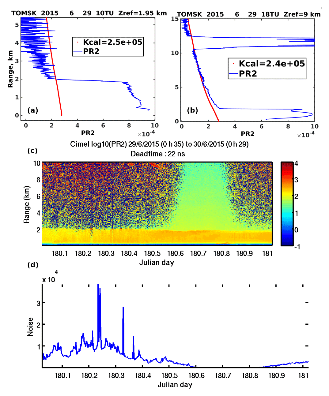
Figure 1Vertical profiles of the attenuated backscatter signal (PR2) for daytime (a) and night-time (b) averaged over 30 min on 29 June 2015 using a calibration constant K to normalize the night-time PR2 to attenuated molecular backscatter at 10 km below the cirrus layer. The red curve is the attenuated molecular backscatter signal. Daily evolution of the vertical profiles of the log10 of the attenuated backscatter (c) and the background signal due to solar radiation (d).
As the alignment of the lidar remains very stable over time, the geometric overlap factor (OF) between the laser and the receiver is estimated between the surface and 500 m by averaging the profiles with a mean attenuated backscatter ratio <1.1 at 500 m and by assuming a constant scattering ratio between the surface and 500 m. This provides a sufficiently accurate geometric overlap factor to correct for the underestimation of the contribution of this altitude domain to the AOD assessment (Fig. 2) between 100 and 500 m. Below 100 m, OF retrieved with this method is not accurate enough and we will assume a constant backscatter ratio between the surface and 100 m. This assumption induces a 2 % error in the AOD assuming a constant extinction layer that is 1000 m deep and a 20 % error in the scattering ratio below 100 m.

Figure 2Geometrical overlap function used for the correction of the lidar data in log10 scale between 100 and 500 m.
2.2 Lidar calibration
Owing to the low SNR of daytime lidar signal above 2–3 km altitude and the difficulty of finding an altitude zone where aerosol backscatter is negligible compared to molecular backscatter, we propose a specific methodology to determine the evolution of the lidar calibration factor. Indeed, a precise calibration of the lidar first allows the determination of the daytime integrated backscatter, assuming very low variation in the calibration factor during the day. Daytime integrated backscatter is then used to derive the integrated lidar ratio using independent AOD measurement from a sun photometer. During the night, calibrated lidar measurements are also useful to reduce the uncertainty in the calculation of the extinction profile to the relative error in the range-corrected signal (PR2) and to that on the determination of the lidar ratio (Appendix A).
A first guess of the calibration coefficient K is obtained from a normalization of the minimum backscatter ratio R to 1 at an altitude between 4 and 9 km for night profiles. The vertical profile of molecular backscatter is estimated from the pressure and temperature profiles after temporal and spatial interpolation of the four daily ERA-Interim ECMWF meteorological fields at 0.75∘ (Dee et al., 2011). The lidar backscatter ratio is averaged over 150 m to reduce the uncertainty in the molecular signal below 2.5 %, i.e. 3.2 times less than the 8 % signal standard deviation shown in Fig. 1 at night at 9 km. A first guess of the aerosol two-way transmittance between the altitude 100 m and the reference altitude zr, chosen for normalization to the backscatter profile, is then calculated after determining the extinction profile with an a priori lidar ratio and using the backward inversion method described in Appendix A. An a priori value of 60 sr is chosen for the vertically averaged lidar ratio S at 808 nm because it corresponds to biomass burning or pollution aerosols using the lidar ratio look up table at 532 nm of the CALIPSO mission aerosol climatology (Omar et al., 2009) and the spectral variability of the lidar ratio between 500 and 808 nm proposed by Cattrall et al. (2005).
The second step in our estimation of lidar calibration is to select the night-time profiles with two additional criteria: zr>7.5 km and . There are 106 such profiles out of 540. This selection increases the probability of having a normalization zone with a good signal-to-noise ratio, a negligible contribution of particle backscatter (zr>7.5 km) and minimization of the normalization error due to an error in when S is very different from 60 sr (0.89). This corresponds to the profile selection shown in the left part of Fig. 4. For these profiles, the calibration factors deduced from a normalization of the PR2 at zr are the best proxies for the lidar calibration. The corresponding optimal values Kopt of the calibration factor are shown in Fig. 3 (black crosses). Since the error in the backscatter ratio at zr is below 3 %, the error, ΔK, in this calibration factor depends mainly on the lidar ratio error, ΔS:
Assuming a 35 % relative uncertainty in S (i.e. expected lidar ratio in the range 35–60 sr assuming that all the aerosol types can be encountered except the clean marine or dusty marine types Omar et al., 2009) and the Cattrall et al. (2005) S spectral variability, the error in Kopt is less than 4 % according to Eq. (1) when 0.89.
The third step is to replace the calibration factors K for non-optimal conditions (daytime profiles, and night-time profiles with either AOD >0.06 or clouds between 4 and 7.5 km) by interpolated values between the nearest Kopt values (see the four arrows labelled with Kopt in Fig. 4). If there are more than 10 days between two optimal calibration factors, the nearest value of Kopt is chosen. If the interpolated value is greater than 20 % of the calibration factor first guess divided by , the latter is retained to take into account exceptionally lower optical transmission of the lidar (window icing, de-tuned filter) or a transient decrease in the emitted energy. Indeed, the use of the interpolated calibration factor would lead to a backscatter ratio much too low in the free troposphere (). There are fewer than 20 such cases between December 2015 and June 2016; therefore fewer than 3 % of the cases studied have an unusually low calibration factor.
The time evolution of K in Fig. 3 shows that the overall transmission of the lidar system increased by 30 % when it was installed in the Fonovaya container in September 2015 and decreased again when it was operated again on the roof of the IAO for 1 month in September 2016. At the Fonovaya site the short-term variability (<10 days) is much higher (>15 %) than at the Tomsk site, where, in contrast, the calibration constant increases regularly by 30 % over 4 months. The short-term variability is mainly related to changes in the optical transmission of the air-conditioned container window, while the drift over 4 months with the initial conditioning of the CE372 on the roof of IAO is due to an improvement in the filter transmission at 808 nm during a gradual increase in outside temperatures. Analysis of the night-time energy measurements does not indicate any significant variation in the energy emitted by the laser diode (<15 %). To estimate our error in K values for non-optimal conditions (red points in Fig. 3), a good proxy is the difference between two optimal calibration factors derived for two observations made with a time difference <1 day. Changes in Kopt for such a short time period cannot be expected when aiming at calibration of daytime observations with night-time calibrated profiles. There are 23 pairs of Kopt values with a 1-day time difference and the standard deviation of their difference, ΔKopt, is 2.5×10⁴. Such a variability is then a limiting factor in our ability to calibrate the lidar for daytime observations or night-time conditions with AOD >0.06 or clouds between 4 and 7.5 km. The corresponding accuracy of the calibration factor K is then of the order of 8 % ().

Figure 3Time evolution from April 2015 to September 2016 of the lidar calibration factor (multiplied by 10−5). Dotted red lines correspond to major changes in lidar housing and expected change in calibration. Black crosses are for nocturnal profiles with molecular normalization at zr>7 km and aerosol two-way transmittance (106 values out of 540). Red dots are for calibration interpolated from optimal conditions. Blue dots are for the few cases (20 out of 540) when calibration cannot be interpolated from optimal conditions.
2.3 Methodology for the lidar aerosol optical depth (AOD) retrieval
Daytime indirect aerosol optical depth retrieval from the calibrated PR2 is based on the well-known backward inversion of PR2 (Fernald, 1984; Klett, 1981) described in Appendix A, provided that an independent measurement of is available to constrain the lidar ratio, e.g. using a sun photometer (Chaikovsky et al., 2016; Cuesta et al., 2008). This work proposes a methodology for the AOD and backscatter ratio profile retrieval, taking into account the different observation conditions described in Fig. 4. It is necessary because the cloud-free lidar profile identified during the 18-month period cannot always be constrained by a sun-photometer AOD, e.g. for night-time observations or daytime observations without the synergy lidar/sun photometer. Two different cases are identified in Fig. 4 for night-time observations. First, a direct AOD retrieval is possible when a layer with molecular signal is found in the upper troposphere above 7.5 km and takes advantage of the good lidar calibration to measure the AOD from the lidar-attenuated backscatter (see Appendix A). For the second case (cloudy conditions 4–7 km or very low AOD <0.04, resulting in a large error in deduced from the attenuated backscatter above 7 km), we cannot rely on an independent estimate of to iterate over the proper lidar ratio. An assumption about the aerosol source must then be made, e.g. using FLEXPART simulations (see Sect. 3), and the lidar ratio is taken from a look-up table for the five main Siberian aerosol sources. This look-up table is representative of Siberia because it is built using all the daytime and night-time observations when independent are available.
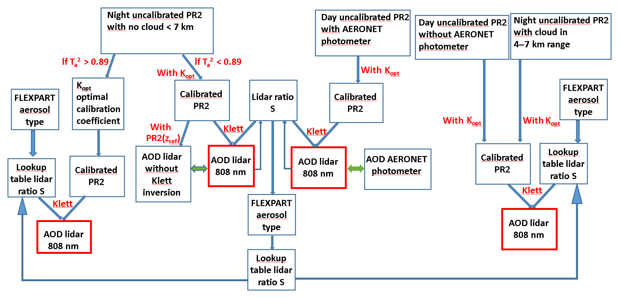
Figure 4Flow chart of the lidar range-corrected signal (PR2) processing to derive the 800 nm aerosol optical depth (AOD) up to the reference altitude (zref). Four different calibrations and AOD calculations are used according to the measurement conditions. Iteration between the AOD calculation and the lidar ratio value is only possible when the AOD is compared to an external AOD reference (green two-sided arrows).
Independent daytime at 808 nm can be obtained using the 870 nm AOD and the Ångström coefficient (AE) measured by the AERONET sun photometer located either at the Tomsk site (56.4∘ N, 85.0∘ E) or that of Tomsk22 (56.4∘ N, 84.1∘ E). Long-range transport of aerosol plumes are generally similar at both sites (Zhuravleva et al., 2017). There are 210 cases out of 539 lidar profiles with coincident lidar and sun-photometer observations.
To increase the number of lidar profiles constrained by an independent estimate of , direct lidar measurements of the 808 nm AOD can also be obtained at night if the lidar is well calibrated and if the reference altitude is above 7.5 km, i.e. with a negligible contribution of particle backscatter (<10 % of molecular backscatter). Indeed, the value of the attenuated backscatter ratio at altitude zr is then a direct measurement of the two-way transmittance ) (Appendix A). The accuracy of the corresponding AOD is % when using the 8 % accuracy for the calibration factor determined in Sect. 2.2. The analysis is limited to AOD >0.04 to avoid large relative errors in the retrieved AOD. There are 63 such cases, providing additional constraint for the lidar ratio retrieval.
Since there is no Raman channel on the CIMEL lidar, it is necessary to assess the likely variability of the aerosol sources to estimate the variability of the lidar ratio. Good knowledge of the aerosol sources linked to the lidar observations will also be beneficial to the analysis of the variability of the backscatter ratio and the AOD discussed in Sects. 5, 6. Back-trajectory analyses are widely used to identify the aerosol sources when the emission areas are well known. Our work is based on a similar approach but the improvement is to use the FLEXible PARTicle dispersion model (FLEXPART) version 9.3 to improve the likelihood of aerosol emission above the lidar site.
3.1 FLEXPART aerosol tracer simulation
FLEXPART is a Lagrangian model designed for computing backward or forward long-range transport, diffusion, dry and wet deposition of air pollutants or aerosol particles from point sources using a large number of particles (Stohl and Seibert, 1998; Stohl et al., 2002). Particle dispersion model calculations can be performed by assuming two modes of transport in the atmosphere: passive transport without removal processes and transport of aerosol tracers, including removal by dry and wet deposition in the cloud and under the cloud (Kristiansen et al., 2016; Stohl et al., 2012). For each lidar profile, the latter was chosen using backward simulations of 10 000 particles released in two altitude zones: (i) 500 m to zaer and (ii) zaer to zmax, zmax being the highest altitude with a scattering ratio R>2 and zaer being the aerosol-weighted altitude calculated with the aerosol backscatter vertical profile.
For dry removal, particle density, aerodynamic diameter and standard deviation of a log-normal distribution were assumed to be 1400 kg m−3, 0.25 µm and 1.25, respectively following Stohl et al. (2013). Below-cloud scavenging is modelled using a wet scavenging coefficient defined as λ=AIB, where A is the wet scavenging coefficient, I the precipitation rate in mm h−1, and B is the factor dependency. We set s−1 and B=0.8. The in-cloud scavenging is simulated using a scavenging coefficient defined as , where H is the cloud thickness in metres. The occurrence of clouds is calculated by FLEXPART using the relative humidity fields. The meteorological fields used for the simulations (including precipitation rates) are ERA-Interim ECMWF field at T255 horizontal resolution (≈80 km) and 61 model vertical levels.
A backward run of the model initialized from the receptor point (the lidar location) provides every 6 h potential emission sensitivity (PES) field in seconds with a vertical resolution of 1000 m and a horizontal resolution of (Seibert and Frank, 2004). These PES fields are generally recombined over a 9-day period, either in the first vertical layer (0–1000 m) to obtain PESsurf or over the first five vertical layers (0–5000 m) to obtain PES0–5 km. The first 12 h before release are excluded to avoid a strong bias by the high PES due to recent local emissions which will mask high PES from remote sources. Examples of PES0–5 km fields are shown in Sect. 5.1.
3.2 Distribution of aerosol sources
Several potential aerosol sources have already been identified for Siberia: (1) urban pollution (Dieudonné et al., 2017; Raut et al., 2017), (2) flaring in the oil and gas industry (Huang and Fu, 2016; Stohl et al., 2013), (3) biomass burning (Teakles et al., 2017; Warneke et al., 2009), (4) dust from central Asian deserts (Gomes and Gillette, 1993; Hofer et al., 2017) and (5) organic aerosols emitted by taiga (Paris et al., 2009). The position of these source zones are coupled with the PES maps calculated by FLEXPART for the aerosol source attribution to a given lidar observation.
The role of urban pollution will be identified by the position of cities of more than 500 000 inhabitants in Russia, Mongolia and Kazakhstan without including emission inventory or seasonal variation of the emissions. We are aware it is a crude assumption for a true aerosol modelling exercise but it is a reasonable criteria for testing the potential effect of urban aerosol on the lidar data.
The biomass-burning emission zones are derived from the daily fire radiative power (FRP) maps provided by NASA Fire Information for Resource Management System (FIRMS) using MODIS (Giglio et al., 2003) and the Visible Infrared Imaging Radiometer Suite (VIIRS) (Schroeder et al., 2014). The FRP is estimated from both MODIS and VIIRS hot spots of the brightness temperature measurements. MCD14ML collection 6 standard quality products and VNP14IMGTDLNRT are used for, respectively, MODIS and VIIRS. The FIRMS data set then provides daytime (MODIS, VIIRS) and night-time (VIIRS) measurements with spatial resolutions of 1 km (MODIS) or 0.375 km (VIIRS). Only FRP values >0.3 GW for MODIS and >0.1 GW for VIIRS are used to identify biomass-burning zones.
To identify continental regions covered by forests and deserts, we use the built-in United States Geological Survey (USGS) 24 category land-use database in the WRF (Weather Research and Forecasting) model. This global land cover database is derived from the Advanced Very High Resolution Radiometer (AVHRR) data with a resolution of 1 km spanning a 12-month period (April 1992–March 1993) (Sertel et al., 2010). The role of dust plumes can be overestimated when using only the land-use map, so it is only considered if neither urban pollution nor biomass burning have been identified.
Russia and Nigeria are the two biggest contributors to gas flaring used at oil and gas production and processing sites. The location of flaring sources is based on the anthropogenic emissions ECLIPSEv4 database (Evaluating the Climate and Air Quality Impacts of Short-Lived pollutants) described in Klimont et al. (2017). This inventory includes, in particular, the gridded methane emissions from gas flaring in the Russian Arctic at a degrees horizontal resolution. A threshold of 50 moles km−2 h−1 has been applied to the methane emissions to select areas that could potentially be defined as flaring sources. Owing to the strong variability of flaring emissions, the role of flaring may be overestimated, so, as for the dust emission, it is only considered if anthropogenic and biomass-burning sources are not identified.
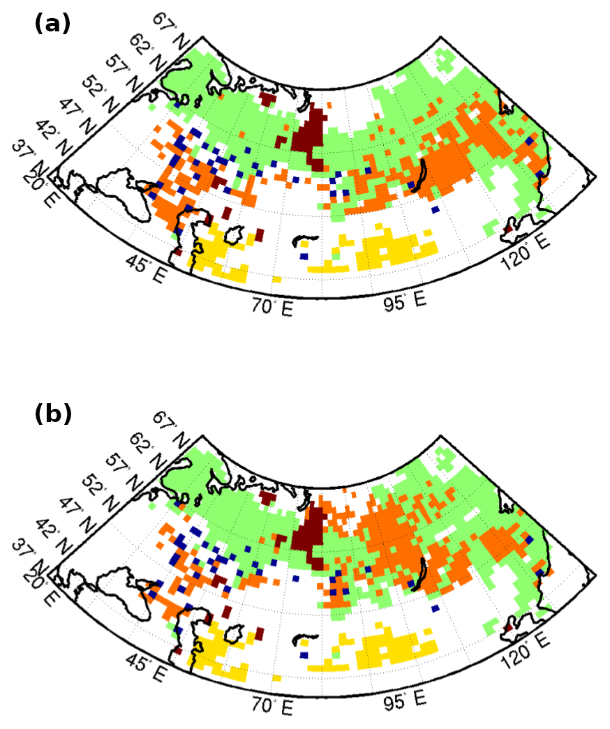
Figure 5Map of the 2015 (a) and 2016 (b) aerosol sources coupled with a FLEXPART PES gridded map: grid cells with large cities (blue square), central Asia desert (yellow), biomass burning (light brown), gas flaring (dark brown) and taiga (green).
The map of the main aerosol emission sources are shown in Fig. 5 for 2015 (top) and 2016 (bottom). The lidar measurement site corresponds to the blue squares at 56∘ N, 85∘ E. In 2016 forest fires were very numerous in central Siberia, whereas they are much further east of Lake Baikal in 2015. When PESsurf>1500 s for at least one grid cell with a large city or flaring emissions, the type of aerosol is classified, respectively, as urban aerosol or flaring aerosol. When PES0–5 km> 1500 s for at least one grid cell with fires or desert soils, the type of aerosol is classified, respectively, as biomass-burning aerosol or dust aerosol. PES0–5 km is chosen for dust and biomass-burning plumes which can be quickly uplifted in the free troposphere up to 5 km. If none of the above conditions are fulfilled, the remaining significant source is the contribution of oxygenated aerosol emission from the very large area covered by the taiga (Zhang et al., 2007).
4.1 Night-time direct AOD measurements
The probability density function (PDF) of the night-time lidar AOD using the direct retrieval method described in Sect. 2.3 is compared with the PDF of the AOD measured during the day by the sun photometer (not including one-third of the sun-photometer AOD <0.04 since AOD <0.04 are not considered in the direct night-time AOD retrieval). The comparison shows that our night-time retrieval using the backscatter ratio at zr gives a realistic distribution of the AOD with similar median and 90th percentiles of the AOD (Fig. 6a, b). A direct comparison between night-time lidar AOD and photometer AOD is not possible in Tomsk because lunar photometry is not available. The alternative solution is to use a sun-photometer AOD with a time difference <6 h with the lidar observations and to include the observed daily variability of the sun-photometer AOD. The correlation plot is also shown in Fig. 6c, showing no clear bias and a satisfactory agreement considering the daily variability of the sun-photometer AOD (error bar in Fig. 6c).

Figure 6(a) PDF of daytime AOD from a sun photometer for lidar measurement days and (b) of night-time AOD calculated with the lidar-attenuated backscatter ratio measurement at the reference altitude zr. N is the number of observations, while p50th and p90th are respectively the median and 90th percentile of the AOD distribution. (c) Correlation plot of night-time lidar AOD versus sun-photometer daytime AOD when the time difference between the two measurements is less than 6 h (35 cases out of 63 night-time lidar AOD). The error bar is the daily variability of the sun-photometer AOD.
4.2 Integrated lidar ratio retrieval
According to Fig. 4, backward inversion of the calibrated lidar-attenuated backscatter can be done iteratively using different lidar ratios when the optical thickness calculated with the extinction profile is compared with the independently obtained AOD. The final solution is always obtained after six iterations. Starting with the largest expected lidar ratio allows a fast convergence towards the true value (e.g. see Young, 1995). Thirteen S808<45 sr out of the 15 FLEXPART dust cases could be retrieved with this method, even though iteration starts with 60 sr. A set of 273 lidar ratios constrained by daytime observations with sun-photometer or by night-time measurements where ) is then available to build the lidar ratio look-up table (Table 1) for each of the five aerosol types determined with the FLEXPART analysis described in Sect. 3 and for three seasons: the cold season (15 October to 15 March), spring (15 March to 30 June) and warm season (30 June to 15 October). The standard deviation of the lidar ratio for each class is a good proxy for the error in the 273 S808 values retrieved with this method. Since the 10 sr error remains significant, it is important to discuss the lidar variability obtained in Table 1. First, as expected (Burton et al., 2012; Omar et al., 2009), the lowest values (40 sr) are indeed obtained for the desert aerosol class, while the highest values (>60 sr) are characteristic of pollution aerosols (flaring and urban pollution in winter). Using the spectral variability of the lidar ratio proposed by Cattrall et al. (2005) to calculate the equivalent S values at 532 nm, S532 is 50 sr for the lower limit of our lidar ratio and 80 sr for the lidar ratio of pollution aerosol. This is consistent with the Burton et al. (2012) analysis, but the lower limit is higher than the average lidar ratio obtained by Hofer et al. (2017) (35 sr) in the deserts of Tajikistan. Aerosol growth and mixing during long-range transport are likely responsible for higher values of S in Tomsk (Ancellet et al., 2016; Nicolae et al., 2013).
For the remaining 267 lidar profiles, where the lidar ratio cannot be constrained by the sun photometer or a good calibrated lidar measurement above 7.5 km, the FLEXPART analysis and the lidar ratio look-up table (Table 1) are used to retrieve the backscatter ratio and the extinction profile (see right- and left-hand side cases in Fig. 4). The relative error in the AOD calculated with the extinction profile is then mainly related to the relative error in the lidar ratio derived from the look-up table, i.e. of the order of 25 %.
Table 1Lidar ratio at 808 nm in sr for the five FLEXPART-derived aerosol types and three seasons (cold, spring and warm) when using independent AOD measurements.

4.3 Lidar AOD seasonal variability
The whole time series of the median of the backscatter ratio R808 between 0–2.5 and 2.5–5 km are shown in Fig. 7. As expected, the mean backscatter ratios >3 are seen mainly in the lowermost troposphere below 2.5 km (22 % of the 540 profiles), while only 5 % are observed for the altitude range 2.5–5 km. Elevated backscatter ratios (>3) are observed from February to September below 2.5 km and from April to September in the free troposphere. The latter is more or less in phase with the start and end dates of dust storm and forest fire periods in Eurasia.

Figure 7Time evolution from April 2015 to September 2016 of the median of the 808 nm Tomsk lidar backscatter ratio for two altitude ranges: 0–2.5 km (b) and 2.5–5 km (a). A, B and C are the cases analysed in Sect. 5.
The time series of the AOD calculated from the extinction vertical profiles is then compared to the AOD from the sun photometer (Fig. 8). The agreement is generally good between the two time series of AOD and elevated AODs (>0.2) are clearly visible at about the same periods. More short-term variability is obtained for the sun-photometer AOD since all 10 min cloud-free observations are shown in Fig. 8. The elevated AOD are not only observed in summer (June to September), which indicates that biomass-burning episodes are not solely responsible for the strong AOD. A strong difference between AOD550 for warm (AOD =0.3) and cold season (AOD =0.08) has been also reported by Chubarova et al. (2016) for the city of Moscow. The corresponding time evolution of the aerosol-weighted altitude calculated with Eq. (2) shows an average altitude of 1.5 km, meaning that the major contribution of the extinction profile to AOD is within the altitude range 0–2.5 km, defined hereafter as the planetary boundary layer (PBL). For periods with elevated AOD, e.g. A, B and C in Fig. 8, zaer=2, 3.5, 1 km, respectively. So zaer>2 km is not only related to an aerosol extinction profile with low AOD.
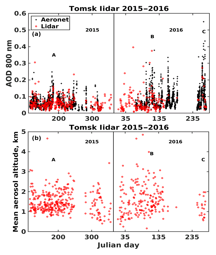
In this section, we focus on the time periods with elevated AOD observed by the AERONET network above Tomsk in order to (1) compare the results of our AOD analysis with AERONET values taken over 48 h around the selected lidar profiles and with satellite data (MODIS or CALIOP), (2) identify the likely aerosol sources derived from the FLEXPART analysis with satellite observations (MODIS, IASI, CALIOP) in the source areas. Looking at Fig. 8, there are five time periods with sun-photometer AOD >0.2: mid-May 2015, the end of May 2015, April 2016, mid-June 2016 and the end of September 2016. We do not have enough lidar data for mid-June 2016. The end of September 2016 and mid-June 2015 cases both correspond to forest fire events, while the end of May 2015 and April 2016 correspond to urban, flaring and dust emissions according to our FLEXPART analysis. Therefore the three time periods corresponding to periods A, B and C of Fig. 8 are analysed in this section. Sect. 5.1 presents the daily variability of the lidar backscatter profiles and sun-photometer AOD, while Sect. 5.2 presents the analysis of satellite observations.
5.1 Lidar data daily variability and comparison with sun-photometer AOD
From 14 to 15 April 2016 (case B in Fig. 8), AOD808 varies between 0.05 and 0.3 for both the lidar and for the sun photometer (Fig. 9a). The vertical profiles of the backscatter ratio (Fig. 10) show a tripling of the aerosol content in the PBL in 12 h which is consistent with the daily variability of the sun-photometer AOD. The comparison of the two night-time lidar profiles also shows a similar increase in the aerosol content between 2.5 and 5 km altitude, which suggests that long-range transport in the aerosol layer took place above the PBL. S808 decreases from 60–70 to 42 sr along with the AOD increase, showing that the increase in aerosol concentrations is the driving factor for the tripling of the AOD. The FLEXPART simulation (Fig. 10) shows strong PES values (>1500 s) northwest of Tomsk over the Ob industrial valley between Tomsk (56∘ N, 85∘ E) and Surgut (62∘ N, 73∘ E) for aerosols detected below 2.5 km. The strong PES values are much more scattered for the upper layer above 2.5 km with aerosol sources both from the lower Ob valley and from a large part of Kazakhstan. Indeed, according to our classification of the type of aerosol, measurements below 2.5 km have been classified as flaring on 14 April, urban on 15 April 03:00 UT and dust on 15 April 16:00 UT. Measurements above 2.5 km were classified as dust emissions. The decrease in S808 is also consistent with a decreasing fraction of pollution aerosol when dust is advected from Kazakhstan (Burton et al., 2012; Hofer et al., 2017).
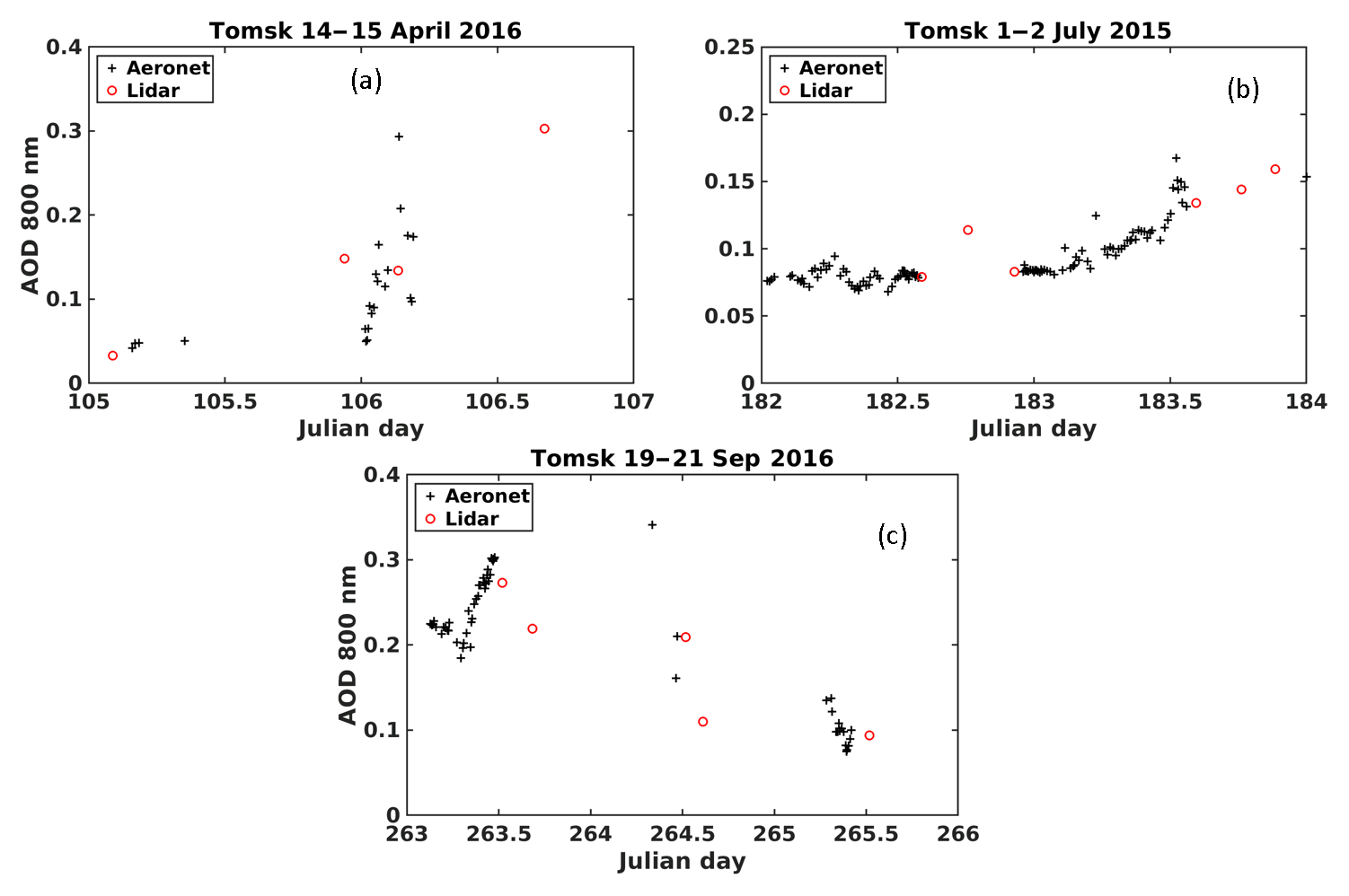
Figure 9Diurnal evolution of the lidar AOD and the sun-photometer AOD at 808 nm for A (b), B (a) and C (c) cases shown in Fig. 8.
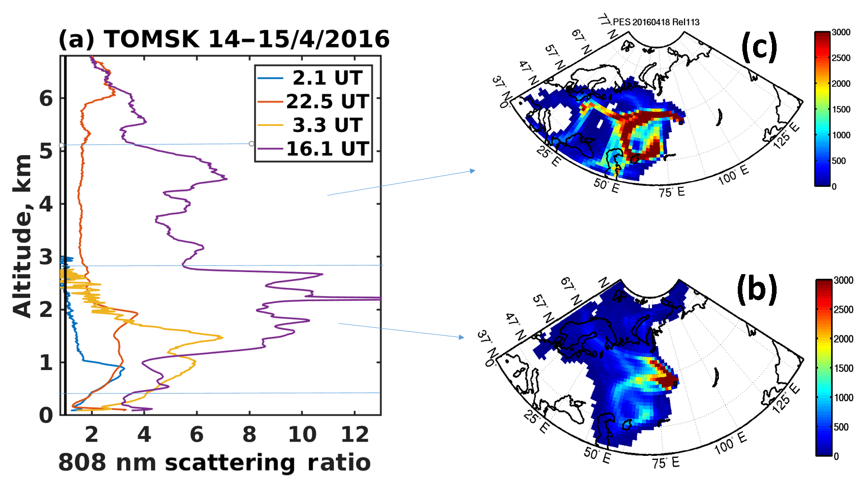
Figure 10Vertical profiles of the scattering ratio on 14 April 2016 at 02:05 and 22:30 UT, and on 15 April 2016 at 03:20 and 16:05 UT (a) and a map of the PES distribution for FLEXPART backward simulation initialized in the PBL (b) and above the PBL (c).
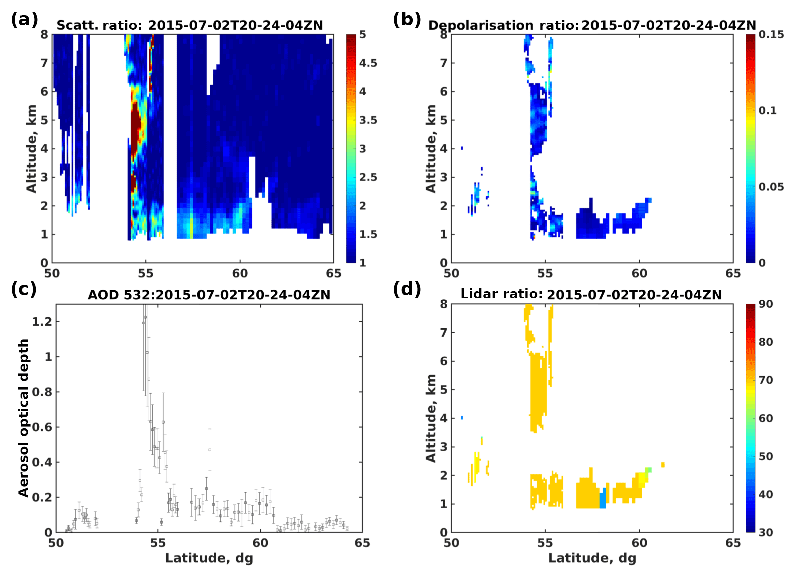
From 30 June to 2 July 2015 (case A in Fig. 8), the measured AOD808 values also gradually increase from 0.08 to 0.16 for both the lidar and the sun photometer (Fig. 9b). The vertical profiles of the backscatter ratio (Fig. 11) show up as in the previous case, with high values (5–7) in the PBL but lower values (≈4) above 2.5 km. S808 increases from 35 to 47 sr, implying that the AOD increase is due both to a change in the aerosol type (40 %) and an increase in the aerosol load (60 %). PES maps indicate an origin still associated with the lower Ob valley for measurements in the PBL (Fig. 11), while high PES values are observed between Tomsk and Lake Baikal for the layer observed in the free troposphere. The Baikal region was impacted by forest fires at the end of June 2015 (see Sect. 5.2), so our classification indeed indicates biomass-burning aerosol for the layer above 2.5 km and a mixture of aerosol produced by flaring (30 June and 1 July) and by biomass burning (2 July) in the PBL. Although the S808 increase is consistent with the advection of biomass-burning aerosol, S808 is surprisingly low (35 sr) for the plume advected at the beginning of the period from the flaring region. One explanation is the strong daily variability of flaring emissions, which cannot be taken into account for our flaring-type attribution only based on advection from the flaring region. S808 of 47 sr is also in the lower range of the expected value for biomass burning, in accordance with the dual air mass origin for the upper layer in Fig. 11, which implies some aerosol mixing.
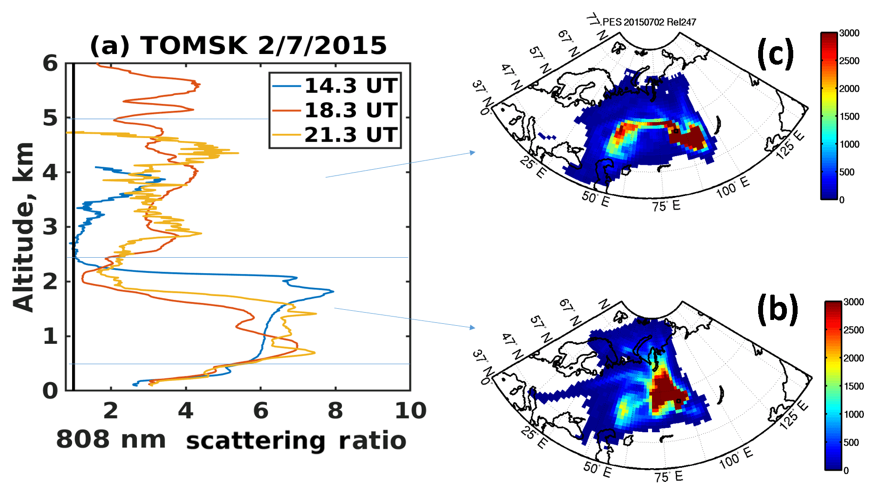
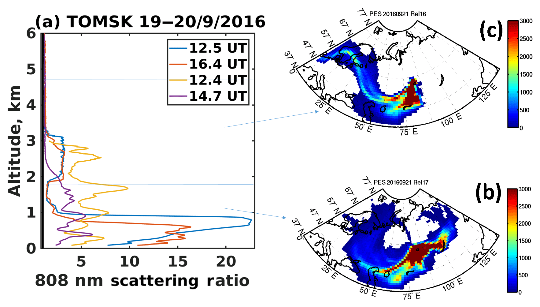
Figure 12As Fig. 10 on 19 September 2016 at 12:30 and 16:25 UT and on 20 September 2016 at 12:25 and 14:40 UT.
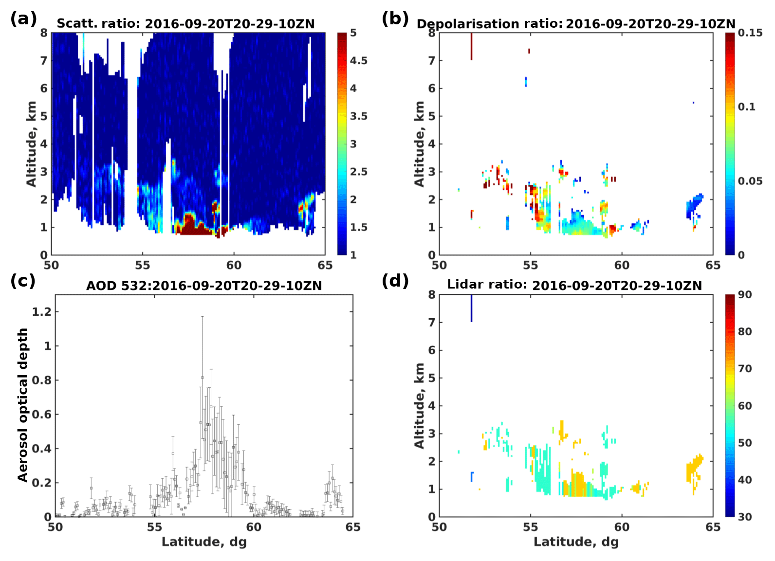
From 19 to 21 September 2016 (case C in Fig. 8), AOD808 values decreased from 0.4 to 0.1 according to the sun photometer and the lidar (Fig. 9c). The vertical profiles of the backscatter ratio (Fig. 12) actually show a very strong decrease in the PBL (20 to 5), with the high values being confined in the 0–800 m altitude range. The aerosol content above 1 km is lower with R808 ranges between 3 and 5. S808 always remains at about 60 sr, except at the end of the 3-day period, where it drops to 40 sr for AOD equal to 0.1. The PES distributions are different from the two previous cases with a large horizontal extension of the area with strong PES values for the PBL (Fig. 12). This area includes a 500 km circle around Tomsk and two branches extending to Lake Baikal and to Kazakhstan. On the contrary, aerosol sources are now confined, for the free troposphere, to a southwest sector above Novosibirsk and Kazakhstan (Fig. 12). For the entire period of 19 to 21 September, aerosols were classified as biomass-burning aerosols due to the presence of forest fires over a large area to the east and north of Tomsk. The 60 sr high values of S808 are consistent with the transport of the biomass burning aerosol from eastern Siberia (Burton et al., 2012), while even the S808 drop to 40 sr is explained by the mixing with air coming from Kazakhstan.
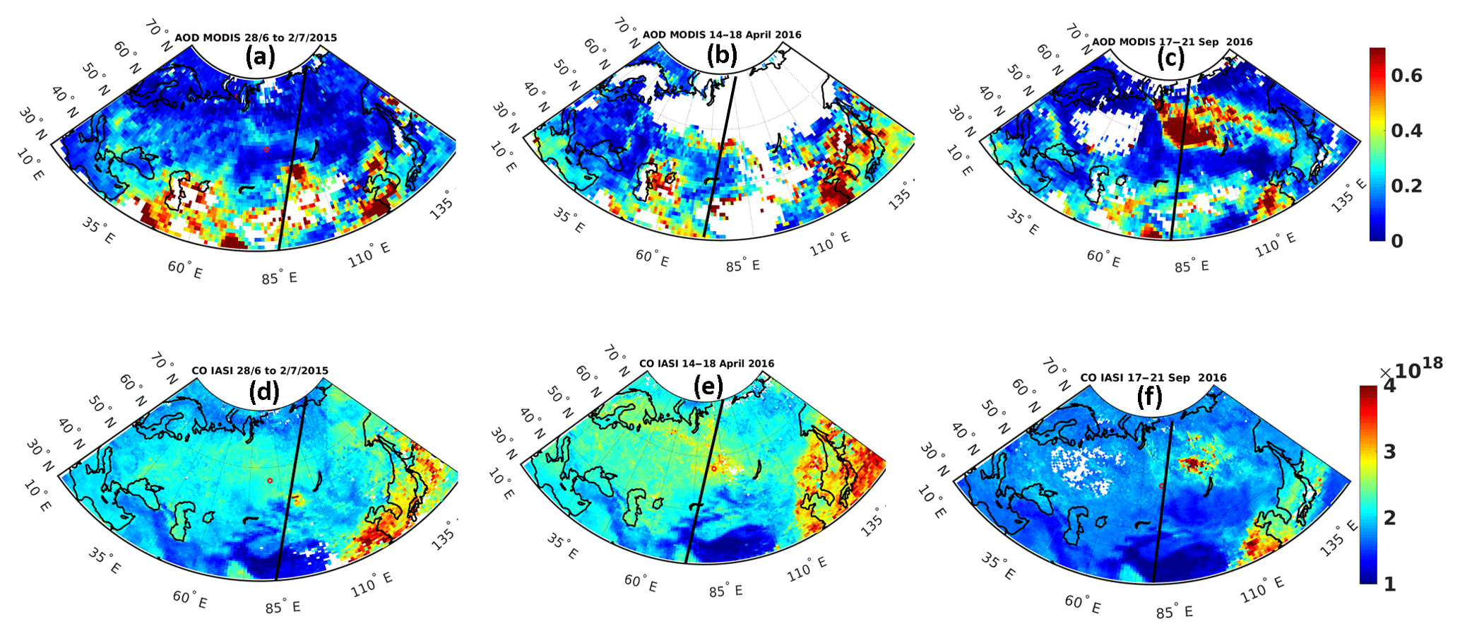
Figure 13Five-day average of AOD at 532 nm from MODIS observations (a, b, c) and of CO in molecules cm−2 from IASI observations (d, e, f) for July 2015 (a, d), April 2016 (b, e) and September 2016 (c, f). The red circle is Tomsk and the thick black lines are the CALIOP overpasses shown in Figs. 14 to 16.
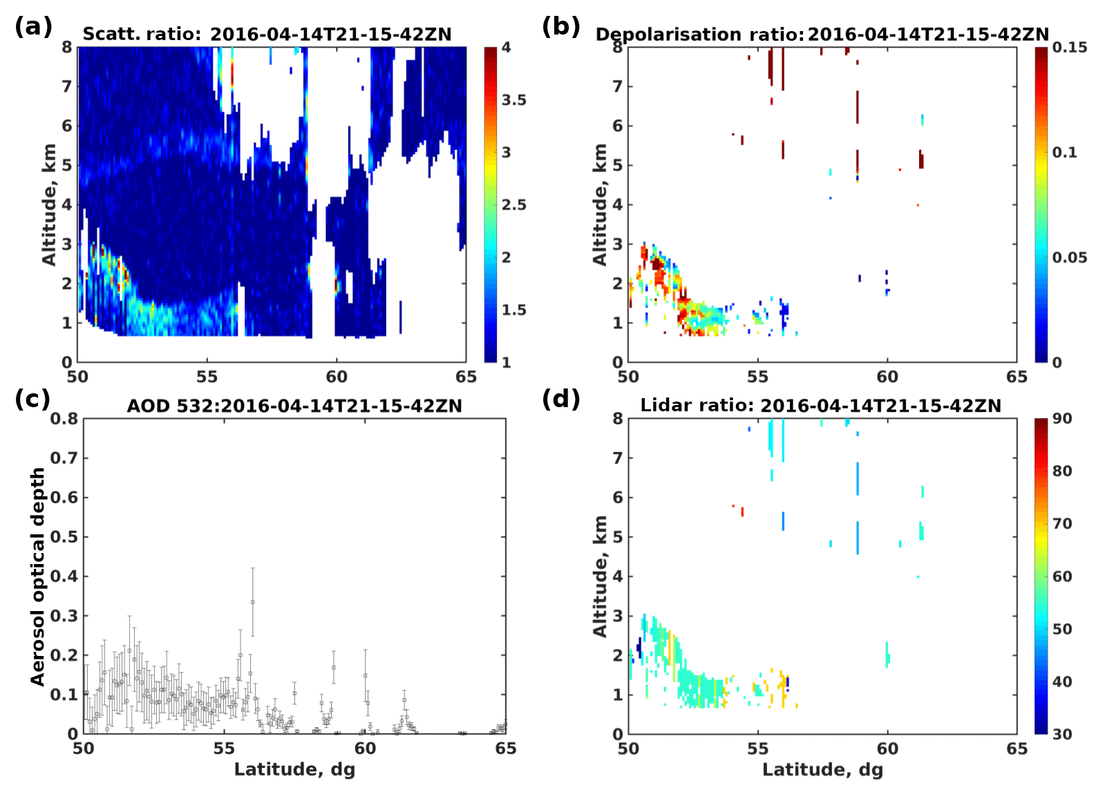
Figure 14Latitudinal cross section of CALIOP 532 nm scattering ratio R532 (a), aerosol depolarization ratio δ532 (b), aerosol optical depth AOD532 (c) and lidar ratio S532 (d) for 14 April 2016.
5.2 Satellite observations
5.2.1 Description of data products
Available satellite observations for these three periods were selected to identify the aerosol source regions. The horizontal distribution of strong AOD is documented by the 550 nm MODIS AOD maps averaged over 5 days. AOD maps are made using the Level-3 MODIS Atmosphere Daily Global Product, which contains roughly 600 statistical data sets sorted into 1 by 1∘ cells on an equal-angle grid that spans a 24 h interval (Levy et al., 2013; Platnick et al., 2015). The role of biomass burning or fuel combustion can be described with a satellite tropospheric CO column measured, for example, by the Infrared Atmospheric Sounding Interferometer (IASI) instrument on Metop A and B. Because a large fraction of atmospheric CO is also related to the oxidation of hydrocarbons including methane, flaring will be a source of CO. The IASI CO data used in this paper have been processed at LATMOS using a retrieval code, FORLI (Fast Optimal Retrievals on Layers for IASI), developed at ULB (Université Libre de Bruxelles) by Hurtmans et al. (2012). Validation for the Siberian and Arctic regions is described in Pommier et al. (2010). The vertical distribution of aerosol layers is inferred from CALIOP overpasses. In this work 532 nm backscatter and depolarization ratios are calculated using the CALIOP level 1 (L1) version 4.10 attenuated backscatter coefficients because they correspond to a better calibration of the lidar data (Vaughan et al., 2012; Winker et al., 2009). They are averaged using a 10 km horizontal resolution and a 60 m vertical resolution. Before horizontal or vertical averaging, the initial 333 m horizontal resolutions (1 km above the altitude 8.2 km) are filtered to remove the cloud layer contribution. This cloud mask makes use of the version 3 level 2 (L2) cloud layer data products (Vaughan et al., 2009) and measurements of the IR imager on the CALIPSO platform. Our scheme for distinguishing between cloud and aerosol is described in Ancellet et al. (2014). To calculate the extinction profile and the optical depth, we use the lidar ratio S532 from the CALIOP version 3 L2 aerosol layer data products (Omar et al., 2009), unless we can calculate the aerosol layer transmittance to constrain S532. To reduce the error when using high horizontal resolution CALIOP profiles, the attenuated backscatter is averaged over 80 km to compute the layer transmittance whenever it is possible. The aerosol depolarization ratio δ532 is also calculated using the perpendicular- to the parallel plus perpendicular polarized aerosol backscatter coefficient (see Appendix B). Whenever it is possible, the use of night-time overpasses are preferred to improve the signal-to-noise ratio (SNR).
5.2.2 Results
From 14 to 18 April 2016, the AOD MODIS and CO IASI maps (Fig. 13b, e) show maxima around the town of Tomsk and more generally in the lower Ob valley (only for IASI insofar as the cloud cover and snow cover do not allow MODIS to be used above 58∘ N). No forest fires were detected during this time period and a predominant role of flaring emissions seems a likely hypothesis for the aerosol layers observed at Tomsk. A CALIPSO overpass with low cloud cover between 50 and 60∘ N is available on 14 April 2016 (thick black line in Fig. 13). The AOD532 observed by CALIOP (Fig. 14) in the range 0.05–0.15 and the associated backscatter ratio (≈2) are lower than the highest values observed by the Tomsk lidar (AOD808≈0.3, e.g. corresponding to AOD532≈0.4 using the sun-photometer AE =0.87), but it is consistent with the range 0.07–0.4 of AOD532 when using the AOD808 observed by the TOMSK lidar. The CALIOP AOD is also lower than the 5-day average MODIS AOD550 (≈0.5) near Tomsk (Fig. 13b), because the CALIOP track was at the edge of the MODIS AOD maxima. The CALIOP observations, however, provide the vertical (0–2 km) and latitudinal (52 to 57∘ N) extent of the aerosol layer due to flaring/urban emissions (Fig. 14), similarly to the Tomsk lidar observations. At latitude below 52∘ N, an aerosol layer is identified as dust by CALIOP with AOD532≈0.2, an upper boundary up to 3 km and depolarization ratio >12 %. The lidar ratio attributed by CALIOP is 55 sr, being consistent with dust emission from Kazakhstan that is responsible for the increasing AOD and advection of the aerosol layer observed in Tomsk above 2.5 km on 15 April 2016.
From 28 June to 2 July 2015, the MODIS AOD and IASI CO maps (Fig. 13a, d) indicate two maxima with both elevated AOD550 and CO values: a forest fire zone of 3.105 km2 at 51∘ N, 97∘ E (AOD550>0.7, i.e. AOD808≈0.3 with AE =2) and the flaring zone in the lower Ob valley between 56 and 65∘ N (AOD550≈0.3, i.e. AOD808≈0.13 with AE =2). This is in rather good agreement with our analysis of aerosol sources, which indicate a mixture of fire and flaring emissions for aerosol layers observed below 2.5 km at Tomsk and the role of fires in the free troposphere above 2.5 km. There is only one CALIPSO overpass on 2 July 2015 (thick black line in Fig. 13) across the fire plume west of Lake Baikal. Elevated AOD532>0.5 are indeed observed by CALIOP at 54∘ N, 97∘ E in smoke layers with very low depolarization ratio (<5 %) and backscatter ratio >5 up to an altitude of 6 km (Fig. 15). The corresponding AOD at 808 nm of the order of 0.18–0.45, when using the 1.9 sun-photometer AE over Tomsk on 2 July 2015, shows that the Tomsk lidar AOD is 2 times lower after being transported from Lake Baikal and mixed with background aerosol. It also explains the 47 sr moderate S808 for a biomass-burning event as discussed in Sect. 5.1. The satellite data analysis for July 2015 is therefore consistent with the results of the Tomsk lidar data processing, both for the AOD range and for the aerosol-type assumption and related lidar ratio.
From 17 to 21 September 2016, the AOD MODIS and CO IASI maps show a very large area impacted by the numerous forest fires (see https://www.fire.uni-freiburg.de/GFMCnew/2016/09/28/20160928_ru.html, last access: 24 November 2017) that took place in Siberia in September 2016. MODIS AOD550>0.7 and CO columns mol cm2 are observed over an area of 1000 km × 1000 km at 57–67∘ N, 95–115∘ E Fig. 13c, d). Tomsk lies just at the edge of this wide plume. The influence of biomass-burning aerosol found in our analysis of Tomsk lidar observations is linked to this event. The CALIPSO track passing over Tomsk and over the fire plume between 56 and 70∘ N (black line in Fig. 13c, d) shows AOD532 in the range 0.4–0.8 between 56 and 60∘ N (Fig. 16). The CALIOP AOD increase corresponds to the MODIS AOD anomaly, although it is 30 % lower than the average MODIS AOD maxima (Fig. 13c). The MODIS AOD is consistent with AOD808>0.4 observed in Tomsk, i.e. a corresponding AOD550=0.75 using AE =1.5 as measured by the Tomsk sun photometer during this time period. The CALIOP depolarization ratio (7 %) is higher than for the July 2015 fire event indicating soil aerosol vertical transport simultaneously with the production of biomass-burning aerosol for these late summer fires (Nisantzi et al., 2014). Similarly the CALIOP lidar ratio (≲70 sr) and the sun-photometer AE (1.5) are lower than the values obtained for the July 2015 fires (S532≈75 sr, AE =1.9) even if these values remain characteristic of a combustion aerosol. The corresponding S808≲53 sr for the 20∕9 CALIOP cross section is lower than S808=60 sr measured for the biomass-burning plume in Tomsk, but the difference is well within the 10 sr expected uncertainty for the Tomsk lidar S808 and the known uncertainties for the CALIOP lidar ratio assessment (Omar et al., 2009). It is also interesting to see that the vertical extent of the fire plume observed by CALIPSO remains fairly low (<1.5 km) between 55 and 60∘ N, i.e. an aerosol plume thickness similar to the Tomsk lidar measurement.
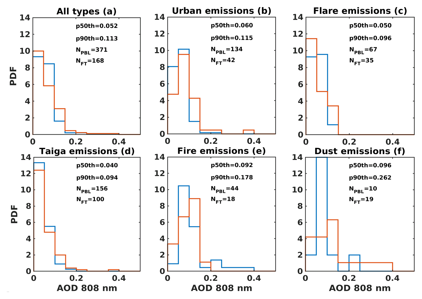
Figure 17PDF of the 808 nm AOD lidar according to the different aerosol types: all (a), urban (b), flaring (c), natural emissions from Siberian forest and grasslands (d), biomass burning (e) and dust (f). Blue PDF is for aerosol-weighted altitude km and red for zaer>1.75 km. NPBL and NFT are respectively the number of PBL only and PBL plus FT observations, while p50th and p90th are respectively the median and 90th percentile of the AOD distribution for both altitude ranges.
The overall conclusion of this section (Sect. 5) is that (1) our approach to attributing an aerosol type to Tomsk lidar observations is validated by a more in-depth study of aerosol sources based on available satellite observations, (2) the AOD and lidar ratio calculated for the Tomsk lidar observations are comparable to the sun-photometer daily AOD variability and satellite AODs in the aerosol source regions identified by the FLEXPART analysis. This will allow the statistical analysis of the lidar measurements according to aerosol types for the 18-month database.
In this section, all observations from April 2015 to October 2016 will be analysed by taking into account the type of aerosol source attributed to each aerosol layer in Sect. 3. The PDFs of AOD at 808 nm have been calculated for the different aerosol types determined with the FLEXPART analysis. To distinguish the AOD distribution for PBL only and PBL plus free tropospheric (FT) aerosol, the PDFs are shown for km and zaer>1.75 km (Fig. 17). The results show that the distribution of AOD when including all aerosol types, has a median value of about 0.05 and a very rapid decrease in the number of observations when AOD >0.1 (90th percentile of about 0.11). If the AOD distributions for the organic aerosol class emitted by vegetation (forest and grassland) and for flaring emissions are not significantly different from the AOD distribution for all types, those for the other classes (urban pollution, biomass burning, dust) have a dominant AOD mode closer to 0.1. The highest 90th percentile (AOD ≥0.18) are for forest fire and dust emissions, although the number of events is statistically lower for these aerosol types than for other emission sources.
The proportions of aerosol types calculated with the number of observations are indeed 41 %, 28 %, 16 %, 10 % and 5 % for forest and grassland emissions, urban pollution, flaring, biomass burning and dust respectively. The dust contribution is very weak as transport pathways and orography significantly reduce the northward transport of central Asian dust plumes. If we consider only AOD >0.1, these relative proportions become very different: 25 %, 25 %, 10 %, 27 % and 13 % for forest and grassland, urban pollution, flaring, vegetation fires and dust respectively. The dust emission contribution to large AOD values now becomes as large as the flaring emission contribution, and the biomass-burning contribution becomes equivalent to urban or forest emissions.
Looking at the differences between PDFs for PBL only (blue) and PBL plus FT (red), the forest and grassland, forest fire and flaring emissions correspond to 60 %–70 % of the AOD measured in PBL while the proportion reaches 76 % for urban emissions and drops to 35 % for dust. This is consistent with urban aerosol emissions associated with the Tomsk–Novosibirsk–Kemerovo triangle being confined below 2.5 km, while dust plumes associated with long-range transport mix little with the boundary layer. It should also be noted that, although forest fire plumes are often associated with long-range transport, their incorporation into the PBL remains effective (70 % of observed cases). Even when AOD is limited to values >0.1, the proportion of biomass-burning aerosol incorporated below 2.5 km remains high (66 %), while that of urban aerosol decreases significantly from 76 % to 53 %.
In conclusion, this study complements several publications (Huang et al., 2010; Sicard et al., 2016) showing that a micropulse lidar is capable of characterizing the variability of the optical properties of aerosols (AOD, vertical profile of the backscatter ratio) at a remote site such as a measuring station in Siberia. In this work, 540 vertical profiles can be used to characterize aerosol sources in Siberia, i.e. 7 times larger than that of the largest lidar database used for dating in Siberia (Samoilova et al., 2012). A total of 300 daytime and 240 night-time profiles of backscatter ratio and AODs have been retrieved over periods of 30 min, after a careful calibration factor analysis. Lidar ratio and AODs are constrained with sun-photometer AODs for 70 % of the daytime lidar measurements, while 26 % of the night-time lidar ratio and AODs greater than 0.04 are constrained by direct lidar measurements at altitudes greater than 7.5 km and where a low aerosol concentration is found. It was complemented by an aerosol source apportionment using the Lagrangian FLEXPART model in order to determine the lidar ratio of the remaining 48 % of the lidar data. FLEXPART simulations are done with an aerosol tracer and aerosol removal processes for five potential sources of aerosol emissions. Comparisons of vertical profiles of the backscatter ratio and AOD at 808 nm with sun-photometer AOD and satellite observations show that (1) our approach to attributing an aerosol type to Tomsk lidar observations is validated using satellite observations for three case studies, (2) the AOD and lidar ratio calculated for the Tomsk lidar observations are comparable to the sun-photometer daily AOD variability in Tomsk and satellite AOD in the source regions identified by the FLEXPART analysis.
According to the analysis of aerosol sources, the occurrence of layers linked to natural emissions (vegetation, forest fires and dust) is high (56 %), but anthropogenic emissions still contribute to 44 % of the detected layers (one-third from flaring and two-thirds from urban emissions). The frequency of dust events is very low (5 %). When only looking at AOD 1, contributions from taiga emissions, forest fires and urban pollution become equivalent (25 %), while those from flaring and dust are lower (10 %–13 %). A major advantage of lidar data in AOD climatological studies is the opportunity to discuss the contribution of different altitude ranges to the large AOD. For example, aerosols related to the urban and flaring emissions remain confined below 2.5 km, while aerosols from dust events are mainly observed above 2.5 km. Aerosols from forest fire emissions are observed to be the opposite, both within and above the PBL.
The FLEXPART code version 9.2 was downloaded from the FLEXPART wiki homepage (https://www.flexpart.eu/downloads, last access: 9 January 2019; see also Stohl et al., 2002).
The CIMEL lidar 372 processed data (AOD, backscatter ratio) are available on the LATMOS data server and can be provided on request. The 18-month calibrated lidar data for Tomsk are available on request at the following ftp address: ftp://ftp.icare.univ-lille1.fr/GROUND-BASED/Tomsk/ (last access: 23 October 2018) The daily MODIS and VIIRS information from the fires were provided by LANCE FIRMS operated by NASA/GSFC/EOSDIS and are available at https://firms.modaps.eosdis.nasa.gov/download/ (last access: 9 January 2019).
The level 3 gridded MODIS aerosol parameter data collection 6 were provided in hdf format by https://ladsweb.modaps.eosdis.nasa.gov/search/order/1/MYD08_D3–61 (see https://doi.org/10.5067/MODIS/MYD08_D3.061, Platnick et al., 2017) and by https://ladsweb.modaps.eosdis.nasa.gov/search/order/1/MOD08_D3–61 (see https://doi.org/10.5067/MODIS/MOD08_D3.061, Platnick et al., 2017) The sun-photometer data for TOMSK have been downloaded from the AERONET database (https://aeronet.gsfc.nasa.gov, last access: 9 January 2019). CALIOP L1 and L2 data were downloaded from the ICARE database (http://www.icare.univ-lille1.fr, last access: 9 January 2019). The IASI CO data were downloaded from the https://doi.org/10.25326/16 web site (Clerbaux, 2018). Meteorological analyses are available at ECMWF (http://www.ecmwf.int, last access: 9 January 2019).
In this appendix, the aerosol optical parameters derived from a backscatter lidar are more precisely described. A backscatter lidar measures the range-corrected lidar signal, Pλ(z), at range z, which can be related to βλ(z) by the following equation:
where Kλ is the range-independent calibration coefficient of the lidar system, T2 is the two-way transmittance due to any scattering (or absorbing) species along the optical path between the scattering volume at range z and the ground, and βλ are the total volume backscatter coefficients at wavelength λ with the subscripts m and a specifying, respectively, molecular and aerosol contributions to the scattering process. For the sake of readability of the text, the reference to λ is now omitted. The two-way transmittance for any constituent, x, is
where τx(z) specifies the optical depth and αx(z) is the volume extinction coefficient. Molecular contribution can be estimated with good accuracy using a molecular density model from ECMWF analysis. When the aerosol contribution is negligible at a range zr in the free troposphere (βa(zr)≪βm(zr) and when τa(zr)<0.05, one can obtain the lidar system constant K:
If we divide P(z) by this value and normalize to the Rayleigh contribution, we obtain the attenuated backscatter ratio, Ratt(z), given by
when τa(zr) is no longer negligible, the backscatter ratio is obtained using the Fernald backward inversion and assuming a range-independent value of the aerosol lidar ratio S (Fernald, 1984):
The assumption of a range-independent aerosol lidar ratio is often not valid (Burton et al., 2012) but it is a well-known method to compute the extinction profile for a single wavelength lidar with no independent measurement of the extinction profile (i.e. with a Raman or a high spectral resolution lidar channel). The error remains weak, provided that two different aerosol layers with similar contributions to the AOD are not simultaneously present. The two-way aerosol transmittance in Eq. (A6) is obtained from an independent AOD daytime measurement or the night-time attenuated backscatter ratio (see Eq. A4) if the aerosol contribution is less than 10 % at zr (i.e. an AOD error of the order of 0.05). When neither of the two previous conditions are met, then is obtained by up to six iterations of Eq. (A6). Independent measurements of AOD or night-time Ratt(zr) can also be used to obtain the integrated lidar ratio S using an iterative calculation where an initial value S808=60 sr is assumed to calculate R(z):
When a linear polarized laser beam is emitted, depolarization related to backscattering in the atmosphere can be measured by a receiving lidar system with an optical selection of the parallel- and cross-polarized signal. The backscatter ratios, R, for perpendicular- and parallel-polarized light are defined as
where is the Rayleigh depolarization, the wavelength dependency of which can be found in Bucholtz (1995), e.g. δm=0.015 at 532 nm. The ratio of the aerosol cross- to parallel-polarized backscatter coefficient is called the aerosol depolarization ratio, δa, given by
where is the total depolarization ratio. The total depolarization ratio δ has the advantage of being less unstable when the aerosol layer is weak and it is also less dependent on instrumental parameters (Cairo et al., 1999). Because the aerosol depolarization is strongly dependent on the accuracy of R532(z), we do not calculate this ratio as R532(z)<1.75
GA, JP and VM designed the lidar data processing methodology. IP, YB and SN designed and carried out the lidar measurement programme in Tomsk. GA carried out the FLEXPART analysis. JCR provided the aerosol source inventories. AZ carried out the case study satellite data analysis of Sect. 5. GA and JP wrote the manuscript with contributions from all co-authors.
The authors declare that they have no conflict of interest.
This work was supported by the CNES EECLAT project, the iCUPE H2020 project and the Chantier Arctique Français (PARCS). The work was also supported in part
by Ministry of Education of Science of RF (agreement no. 14.616.21.0104, unique identifier
RFMEFI61618X0104).
We thank the European Centre for Medium Range Weather Forecasts (ECMWF) for the provision of ERA-Interim reanalysis data and
the FLEXPART development team for the provision of the FLEXPART 9.2 model version used in this publication.
The authors thank the AERIS infrastructure and NASA/GSFC for providing the satellite data used in this paper (CO, AOD, CALIOP and fire
FRP).
Edited by: Thomas Eck
Reviewed by: two anonymous referees
AMAP: Assessment 2015: Black carbon and ozone as Arctic climate forcers. Arctic Monitoring and Assessment Programme (AMAP), 1–116, Arctic Monitoring and Assessment Programme (AMAP), Oslo, Norway, available at: https://www.amap.no/documents/doc/AMAP-Assessment-2015-Black-carbon-and-ozone-as-Arctic, last access: 30 November 2015. a
Ancellet, G., Pelon, J., Blanchard, Y., Quennehen, B., Bazureau, A., Law, K. S., and Schwarzenboeck, A.: Transport of aerosol to the Arctic: analysis of CALIOP and French aircraft data during the spring 2008 POLARCAT campaign, Atmos. Chem. Phys., 14, 8235–8254, https://doi.org/10.5194/acp-14-8235-2014, 2014. a, b
Ancellet, G., Pelon, J., Totems, J., Chazette, P., Bazureau, A., Sicard, M., Di Iorio, T., Dulac, F., and Mallet, M.: Long-range transport and mixing of aerosol sources during the 2013 North American biomass burning episode: analysis of multiple lidar observations in the western Mediterranean basin, Atmos. Chem. Phys., 16, 4725–4742, https://doi.org/10.5194/acp-16-4725-2016, 2016. a
Ansmann, A., Wagner, F., Althausen, D., Müller, D., Herber, A., and Wandinger, U.: European pollution outbreaks during ACE 2: Lofted aerosol plumes observed with Raman lidar at the Portuguese coast, J. Geophys. Res.-Atmos., 106, 20725–20733, https://doi.org/10.1029/2000JD000091, 2001. a
Arnold, S. R., Law, K. S., Brock, C. A., Thomas, J. L., Starkweather, S. M., Salzen, K. Von, Stohl, A., Sharma, S., Lund, M., Flanner, M., Petäjä, T., Tanimoto, H., Gamble, J., Dibb, J., Melamed, M., Johnson, M., Fidel, M., Tynkkynen, V., Baklanov, A., Eckhardt, S., Monks, S., Browse, J., and Bozem, H.: Arctic air pollution: Challenges and opportunities for the next decade, Elem. Sci. Anth., 4, 1–17, https://doi.org/10.12952/journal.elementa.000104, 2016. a
Bond, T. C., Doherty, S. J., Fahey, D. W., Forster, P. M., Berntsen, T., DeAngelo, B. J., Flanner, M. G., Ghan, S., Kärcher, B., Koch, D., Kinne, S., Kondo, Y., Quinn, P. K., Sarofim, M. C., Schultz, M. G., Schulz, M., Venkataraman, C., Zhang, H., Zhang, S., Bellouin, N., Guttikunda, S. K., Hopke, P. K., Jacobson, M. Z., Kaiser, J. W., Klimont, Z., Lohmann, U., Schwarz, J. P., Shindell, D., Storelvmo, T., Warren, S. G., and Zender, C. S.: Bounding the role of black carbon in the climate system: A scientific assessment, J. Geophys. Res.-Atmos., 118, 5380–5552, https://doi.org/10.1002/jgrd.50171, 2013. a
Bucholtz, A.: Rayleigh-scattering calculations for the terrestrial atmosphere, Appl. Opt., 34, 2765–2773, https://doi.org/10.1364/AO.34.002765, 1995. a
Burton, S. P., Ferrare, R. A., Hostetler, C. A., Hair, J. W., Rogers, R. R., Obland, M. D., Butler, C. F., Cook, A. L., Harper, D. B., and Froyd, K. D.: Aerosol classification using airborne High Spectral Resolution Lidar measurements – methodology and examples, Atmos. Meas. Tech., 5, 73–98, https://doi.org/10.5194/amt-5-73-2012, 2012. a, b, c, d, e
Cairo, F., Donfrancesco, G. D., Adriani, A., Pulvirenti, L., and Fierli, F.: Comparison of Various Linear Depolarization Parameters Measured by Lidar, Appl. Opt., 38, 4425–4432, 1999. a
Campbell, J. R., Hlavka, D. L., Welton, E. J., Flynn, C. J., Turner, D. D., Spinhirne, J. D., III, V. S. S., and Hwang, I. H.: Full-Time, Eye-Safe Cloud and Aerosol Lidar Observation at Atmospheric Radiation Measurement Program Sites: Instruments and Data Processing, J. Atmos. Ocean. Tech., 19, 431–442, https://doi.org/10.1175/1520-0426(2002)019<0431:FTESCA>2.0.CO;2, 2002. a
Cattrall, C., Reagan, J., Thome, K., and Dubovik, O.: Variability of aerosol and spectral lidar and backscatter and extinction ratios of key aerosol types derived from selected Aerosol Robotic Network locations, J. Geophys. Res., 110, D10S11, https://doi.org/10.1029/2004JD005124, 2005. a, b, c
Chaikovsky, A., Ivanov, A., Balin, Y., Elnikov, A., Tulinov, G., Plusnin, I., Bukin, O., and Chen, B.: Lidar network CIS-LiNet for monitoring aerosol and ozone in CIS regions, Proc. SPIE, 6160, 9 pp., https://doi.org/10.1117/12.675920, 2006. a
Chaikovsky, A., Dubovik, O., Holben, B., Bril, A., Goloub, P., Tanré, D., Pappalardo, G., Wandinger, U., Chaikovskaya, L., Denisov, S., Grudo, J., Lopatin, A., Karol, Y., Lapyonok, T., Amiridis, V., Ansmann, A., Apituley, A., Allados-Arboledas, L., Binietoglou, I., Boselli, A., D'Amico, G., Freudenthaler, V., Giles, D., Granados-Muñoz, M. J., Kokkalis, P., Nicolae, D., Oshchepkov, S., Papayannis, A., Perrone, M. R., Pietruczuk, A., Rocadenbosch, F., Sicard, M., Slutsker, I., Talianu, C., De Tomasi, F., Tsekeri, A., Wagner, J., and Wang, X.: Lidar-Radiometer Inversion Code (LIRIC) for the retrieval of vertical aerosol properties from combined lidar/radiometer data: development and distribution in EARLINET, Atmos. Meas. Tech., 9, 1181–1205, https://doi.org/10.5194/amt-9-1181-2016, 2016. a, b
Chubarova, N. Y., Poliukhov, A. A., and Gorlova, I. D.: Long-term variability of aerosol optical thickness in Eastern Europe over 2001–2014 according to the measurements at the Moscow MSU MO AERONET site with additional cloud and NO2 correction, Atmos. Meas. Tech., 9, 313–334, https://doi.org/10.5194/amt-9-313-2016, 2016. a
Clerbaux, C.: Daily IASI/Metop-A ULB-LATMOS carbon monoxide (CO) L2 product (total column), [Data set], AERIS, https://doi.org/10.25326/16, 2018 a
Cuesta, J., Flamant, P. H., and Flamant, C.: Synergetic technique combining elastic backscatter lidar data and sunphotometer AERONET inversion for retrieval by layer of aerosol optical and microphysical properties, Appl. Opt., 47, 4598–4611, https://doi.org/10.1364/AO.47.004598, 2008. a, b
Dee, D. P., Uppala, S. M., Simmons, A. J., Berrisford, P., Poli, P., Kobayashi, S., Andrae, U., Balmaseda, M. A., Balsamo, G., Bauer, P., Bechtold, P., Beljaars, A. C. M., van de Berg, L., Bidlot, J., Bormann, N., Delsol, C., Dragani, R., Fuentes, M., Geer, A. J., Haimberger, L., Healy, S. B., Hersbach, H., Hólm, E. V., Isaksen, L., Kållberg, P., Köhler, M., Matricardi, M., McNally, A. P., Monge-Sanz, B. M., Morcrette, J.-J., Park, B.-K., Peubey, C., de Rosnay, P., Tavolato, C., Thépaut, J.-N., and Vitart, F.: The ERA-Interim reanalysis: configuration and performance of the data assimilation system, Q. J. Roy. Meteor. Soc., 137, 553–597, https://doi.org/10.1002/qj.828, 2011. a
Di Biagio, C., Pelon, J., Ancellet, G., Bazureau, A., and Mariage, V.: Sources, Load, Vertical Distribution, and Fate of Wintertime Aerosols North of Svalbard From Combined V4 CALIOP Data, Ground-Based IAOOS Lidar Observations and Trajectory Analysis, J. Geophys. Res.-Atmos., 123, 1363–1383, https://doi.org/10.1002/2017JD027530, 2018. a
Dieudonné, E., Ravetta, F., Pelon, J., Goutail, F., and Pommereau, J.-P.: Linking NO2 surface concentration and integrated content in the urban developed atmospheric boundary layer, Geophys. Res. Lett., 40, 1247–1251, https://doi.org/10.1002/grl.50242, 2013. a
Dieudonné, E., Chazette, P., Marnas, F., Totems, J., and Shang, X.: Lidar profiling of aerosol optical properties from Paris to Lake Baikal (Siberia), Atmos. Chem. Phys., 15, 5007–5026, https://doi.org/10.5194/acp-15-5007-2015, 2015. a
Dieudonné, E., Chazette, P., Marnas, F., Totems, J., and Shang, X.: Raman Lidar Observations of Aerosol Optical Properties in 11 Cities from France to Siberia, Remote Sens., 9, 978, https://doi.org/10.3390/rs9100978, 2017. a
Di Pierro, M., Jaeglé, L., Eloranta, E. W., and Sharma, S.: Spatial and seasonal distribution of Arctic aerosols observed by the CALIOP satellite instrument (2006–2012), Atmos. Chem. Phys., 13, 7075–7095, https://doi.org/10.5194/acp-13-7075-2013, 2013. a
Eckhardt, S., Quennehen, B., Olivié, D. J. L., Berntsen, T. K., Cherian, R., Christensen, J. H., Collins, W., Crepinsek, S., Daskalakis, N., Flanner, M., Herber, A., Heyes, C., Hodnebrog, Ø., Huang, L., Kanakidou, M., Klimont, Z., Langner, J., Law, K. S., Lund, M. T., Mahmood, R., Massling, A., Myriokefalitakis, S., Nielsen, I. E., Nøjgaard, J. K., Quaas, J., Quinn, P. K., Raut, J.-C., Rumbold, S. T., Schulz, M., Sharma, S., Skeie, R. B., Skov, H., Uttal, T., von Salzen, K., and Stohl, A.: Current model capabilities for simulating black carbon and sulfate concentrations in the Arctic atmosphere: a multi-model evaluation using a comprehensive measurement data set, Atmos. Chem. Phys., 15, 9413–9433, https://doi.org/10.5194/acp-15-9413-2015, 2015. a
Fernald, F. G.: Analysis of atmospheric lidar observations: some comments, Appl. Opt., 23, 652–653, https://doi.org/10.1364/AO.23.000652, 1984. a, b
Giglio, L., Descloitres, J., Justice, C. O., and Kaufman, Y. J.: An Enhanced Contextual Fire Detection Algorithm for MODIS, Remote Sens. Environ., 87, 273–282, https://doi.org/10.1016/S0034-4257(03)00184-6, 2003. a
Gomes, L. and Gillette, D. A.: A comparison of characteristics of aerosol from dust storms in Central Asia with soil-derived dust from other regions, Atmos. Environ. A-Gen., 27, 2539–2544, https://doi.org/10.1016/0960-1686(93)90027-V, 1993. a
Hofer, J., Althausen, D., Abdullaev, S. F., Makhmudov, A. N., Nazarov, B. I., Schettler, G., Engelmann, R., Baars, H., Fomba, K. W., Müller, K., Heinold, B., Kandler, K., and Ansmann, A.: Long-term profiling of mineral dust and pollution aerosol with multiwavelength polarization Raman lidar at the Central Asian site of Dushanbe, Tajikistan: case studies, Atmos. Chem. Phys., 17, 14559–14577, https://doi.org/10.5194/acp-17-14559-2017, 2017. a, b, c
Holben, B., Eck, T., Slutsker, I., Tanré, D., Buis, J., Setzer, A., Vermote, E., Reagan, J., Kaufman, Y., Nakajima, T., Lavenu, F., Jankowiak, I., and Smirnov, A.: AERONET-A Federated Instrument Network and Data Archive for Aerosol Characterization, Remote Sens. Environ., 66, 1–16, https://doi.org/10.1016/S0034-4257(98)00031-5, 1998. a
Huang, K. and Fu, J. S.: A global gas flaring black carbon emission rate dataset from 1994 to 2012, Scientific Data, 3, 160104, https://doi.org/10.1038/sdata.2016.104, 2016. a
Huang, K., Fu, J. S., Prikhodko, V. Y., Storey, J. M., Romanov, A., Hodson, E. L., Cresko, J., Morozova, I., Ignatieva, Y., and Cabaniss, J.: Russian anthropogenic black carbon: Emission reconstruction and Arctic black carbon simulation, J. Geophys. Res.-Atmos., 120, 2015. a
Huang, Z., Huang, J., Bi, J., Wang, G., Wang, W., Fu, Q., Li, Z., Tsay, S., and Shi, J.: Dust aerosol vertical structure measurements using three MPL lidars during 2008 China-U.S. joint dust field experiment, J. Geophys. Res.-Atmos., 115, D00K15, https://doi.org/10.1029/2009JD013273, 2010. a
Hurtmans, D., Coheur, P., Wespes, C., Clarisse, L., Scharf, O., Clerbaux, C., Hadji-Lazaro, J., George, M., and Turquety, S.: FORLI radiative transfer and retrieval code for IASI, J. Quant. Spectrosc. Ra., 113, 1391–1408, https://doi.org/10.1016/j.jqsrt.2012.02.036, 2012. a
Kahn, R. A. and Gaitley, B. J.: An analysis of global aerosol type as retrieved by MISR, J. Geophys. Res.-Atmos., 120, 4248–4281, https://doi.org/10.1002/2015JD023322, 2015. a
Klett, J.: Stable analytical inversion solution for processing lidar returns, Appl. Opt., 20, 211–220, 1981. a
Klimont, Z., Kupiainen, K., Heyes, C., Purohit, P., Cofala, J., Rafaj, P., Borken-Kleefeld, J., and Schöpp, W.: Global anthropogenic emissions of particulate matter including black carbon, Atmos. Chem. Phys., 17, 8681–8723, https://doi.org/10.5194/acp-17-8681-2017, 2017. a
Kristiansen, N. I., Stohl, A., Olivié, D. J. L., Croft, B., Søvde, O. A., Klein, H., Christoudias, T., Kunkel, D., Leadbetter, S. J., Lee, Y. H., Zhang, K., Tsigaridis, K., Bergman, T., Evangeliou, N., Wang, H., Ma, P.-L., Easter, R. C., Rasch, P. J., Liu, X., Pitari, G., Di Genova, G., Zhao, S. Y., Balkanski, Y., Bauer, S. E., Faluvegi, G. S., Kokkola, H., Martin, R. V., Pierce, J. R., Schulz, M., Shindell, D., Tost, H., and Zhang, H.: Evaluation of observed and modelled aerosol lifetimes using radioactive tracers of opportunity and an ensemble of 19 global models, Atmos. Chem. Phys., 16, 3525–3561, https://doi.org/10.5194/acp-16-3525-2016, 2016. a
Law, K. S., Stohl, A., Quinn, P. K., Brock, C. A., Burkhart, J. F., Paris, J.-D., Ancellet, G., Singh, H. B., Roiger, A., Schlager, H., Dibb, J., Jacob, D. J., Arnold, S. R., Pelon, J., and Thomas, J. L.: Arctic Air Pollution: New Insights from POLARCAT-IPY, B. Am. Meteorol. Soc., 95, 1873–1895, https://doi.org/10.1175/BAMS-D-13-00017.1, 2014. a
Levy, R. C., Mattoo, S., Munchak, L. A., Remer, L. A., Sayer, A. M., Patadia, F., and Hsu, N. C.: The Collection 6 MODIS aerosol products over land and ocean, Atmos. Meas. Tech., 6, 2989–3034, https://doi.org/10.5194/amt-6-2989-2013, 2013. a, b
Marenco, F., Santacesaria, V., Bais, A. F., Balis, D., di Sarra, A., Papayannis, A., and Zerefos, C.: Optical properties of tropospheric aerosols determined by lidar andspectrophotometric measurements (Photochemical Activity and Solar UltravioletRadiation campaign), Appl. Opt., 36, 6875–6886, https://doi.org/10.1364/AO.36.006875, 1997. a
Mariage, V., Pelon, J., Blouzon, F., Victori, S., Geyskens, N., Amarouche, N., Drezen, C., Guillot, A., Calzas, M., Garracio, M., Wegmuller, N., Sennéchael, N., and Provost, C.: IAOOS microlidar-on-buoy development and first atmospheric observations obtained during 2014 and 2015 arctic drifts, Opt. Express, 25, A73–A84, https://doi.org/10.1364/OE.25.000A73, 2017. a, b, c, d
Mattis, I., Ansmann, A., Müller, D., Wandinger, U., and Althausen, D.: Multiyear aerosol observations with dual-wavelength Raman lidar in the framework of EARLINET, J. Geophys. Res.-Atmos., 109, D13203, https://doi.org/10.1029/2004JD004600, 2004. a
Mishra, A. K., Koren, I., and Rudich, Y.: Effect of aerosol vertical distribution on aerosol-radiation interaction: A theoretical prospect, Heliyon, 1, e00036, https://doi.org/10.1016/j.heliyon.2015.e00036, 2015. a
Misra, A., Tripathi, S. N., Kaul, D. S., and Welton, E. J.: Study of MPLNET-Derived Aerosol Climatology over Kanpur, India, and Validation of CALIPSO Level 2 Version 3 Backscatter and Extinction Products, J. Atmos. Ocean. Tech., 29, 1285–1294, https://doi.org/10.1175/JTECH-D-11-00162.1, 2012. a
Nicolae, D., Nemuc, A., Mueller, D., Talianu, C., Vasilescu, J., Belegante, L., and Kolgotin, A.: Characterization of fresh and aged biomass burning events using multiwavelength Raman lidar and mass spectrometry, J. Geophys. Res.-Atmos., 118, 2956–2965, https://doi.org/10.1002/jgrd.50324, 2013. a
Nisantzi, A., Mamouri, R. E., Ansmann, A., and Hadjimitsis, D.: Injection of mineral dust into the free troposphere during fire events observed with polarization lidar at Limassol, Cyprus, Atmos. Chem. Phys., 14, 12155–12165, https://doi.org/10.5194/acp-14-12155-2014, 2014. a
Omar, A., Winker, D., Kittaka, C., Vaughan, M., Liu, Z., Hu, Y., Trepte, C., Rogers, R., Ferrare, R., Lee, K., Kuehn, R., and Hostetler, C.: The CALIPSO Automated Aerosol Classification and Lidar Ratio Selection Algorithm, J. Atmos. Ocean. Tech., 26, 1994–2014, https://doi.org/10.1175/2009JTECHA1231.1, 2009. a, b, c, d, e, f
Pappalardo, G., Amodeo, A., Apituley, A., Comeron, A., Freudenthaler, V., Linné, H., Ansmann, A., Bösenberg, J., D'Amico, G., Mattis, I., Mona, L., Wandinger, U., Amiridis, V., Alados-Arboledas, L., Nicolae, D., and Wiegner, M.: EARLINET: towards an advanced sustainable European aerosol lidar network, Atmos. Meas. Tech., 7, 2389–2409, https://doi.org/10.5194/amt-7-2389-2014, 2014. a
Paris, J.-D., Arshinov, M. Y., Ciais, P., Belan, B. D., and Nédélec, P.: Large-scale aircraft observations of ultra-fine and fine particle concentrations in the remote Siberian troposphere: New particle formation studies, Atmos. Environ., 43, 1302–1309, https://doi.org/10.1016/j.atmosenv.2008.11.032, 2009. a
Pelon, J., Mallet, M., Mariscal, A., Goloub, P., Tanré, D., Bou Karam, D., Flamant, C., Haywood, J., Pospichal, B., and Victori, S.: Microlidar observations of biomass burning aerosol over Djougou (Benin) during African Monsoon Multidisciplinary Analysis Special Observation Period 0: Dust and Biomass-Burning Experiment, J. Geophys. Res.-Atmos., 113, D00C18, https://doi.org/10.1029/2008JD009976, 2008. a, b
Platnick, S., Hubanks, P., Meyer, K., and King, M. D.: MODIS Atmosphere L3 Daily Product, Goddard Space Flight Center, USA, https://doi.org/10.5067/MODIS/MOD08_D3.006, 2015. a
Platnick, S. et al.: MODIS Atmosphere L3 Daily Product, NASA MODIS Adaptive Processing System, Goddard Space Flight Center, USA, https://doi.org/10.5067/MODIS/MOD08_D3.061, 2017 a, b
Pommier, M., Law, K. S., Clerbaux, C., Turquety, S., Hurtmans, D., Hadji-Lazaro, J., Coheur, P.-F., Schlager, H., Ancellet, G., Paris, J.-D., Nédélec, P., Diskin, G. S., Podolske, J. R., Holloway, J. S., and Bernath, P.: IASI carbon monoxide validation over the Arctic during POLARCAT spring and summer campaigns, Atmos. Chem. Phys., 10, 10655–10678, https://doi.org/10.5194/acp-10-10655-2010, 2010. a
Raut, J.-C., Marelle, L., Fast, J. D., Thomas, J. L., Weinzierl, B., Law, K. S., Berg, L. K., Roiger, A., Easter, R. C., Heimerl, K., Onishi, T., Delanoë, J., and Schlager, H.: Cross-polar transport and scavenging of Siberian aerosols containing black carbon during the 2012 ACCESS summer campaign, Atmos. Chem. Phys., 17, 10969–10995, https://doi.org/10.5194/acp-17-10969-2017, 2017. a
Samoilova, S. V., Balin, Y. S., Kokhanenko, G. P., and Penner, I. E.: Investigation of the vertical distribution of tropospheric aerosol layers from multifrequency laser sensing data. Part 2: The vertical distribution of optical aerosol characteristics in the visible region, Atmos. Ocean. Opt., 23, 95–105, https://doi.org/10.1134/S102485601002003X, 2010. a
Samoilova, S. V., Balin, Y. S., Kokhanenko, G. P., and Penner, I. E.: Investigation of the vertical distribution of tropospheric aerosol layers using the data of multiwavelength lidar sensing. Part 3. Spectral peculiarities of the vertical distribution of the aerosol optical characteristics, Atmos. Ocean. Opt., 25, 208–215, https://doi.org/10.1134/S1024856012030098, 2012. a, b
Schroeder, W., Oliva, P., Giglio, L., and Csiszar, I. A.: The New VIIRS 375m active fire detection data product: Algorithm description and initial assessment, Remote Sens. Environ., 143, 85–96, https://doi.org/10.1016/j.rse.2013.12.008, 2014. a, b
Seibert, P. and Frank, A.: Source-receptor matrix calculation with a Lagrangian particle dispersion model in backward mode, Atmos. Chem. Phys., 4, 51–63, https://doi.org/10.5194/acp-4-51-2004, 2004. a
Sertel, E., Robock, A., and Ormeci, C.: Impacts of land cover data quality on regional climate simulations, Int. J. Climatol., 30, 1942–1953, https://doi.org/10.1002/joc.2036, 2010. a
Sicard, M., Izquierdo, R., Alarcón, M., Belmonte, J., Comerón, A., and Baldasano, J. M.: Near-surface and columnar measurements with a micro pulse lidar of atmospheric pollen in Barcelona, Spain, Atmos. Chem. Phys., 16, 6805–6821, https://doi.org/10.5194/acp-16-6805-2016, 2016. a
Stocker, T., Qin, D., Plattner, G., Tignor, M., Allen, S., Boschung, J., Nauels, A., Xia, Y., Bex, V., and Midgley, P. (Eds.): Index, book section Index, 1523–1535, Cambridge University Press, Cambridge, United Kingdom and New York, NY, USA, https://doi.org/10.1017/CBO9781107415324, 2013. a, b
Stohl, A. and Seibert, P.: Accuracy of trajectories as determined from the conservation of meteorological tracers, Q. J. Roy. Meteor. Soc., 124, 1465–1484, 1998. a
Stohl, A., Eckhardt, S., Forster, C., James, P., Spichtinger, N., and Seibert, P.: A replacement for simple back trajectory calculations in the interpretation of atmospheric trace substance measurements, Atmos. Environ., 36, 4635–4648, https://doi.org/10.1016/S1352-2310(02)00416-8, 2002. a, b
Stohl, A., Seibert, P., Wotawa, G., Arnold, D., Burkhart, J. F., Eckhardt, S., Tapia, C., Vargas, A., and Yasunari, T. J.: Xenon-133 and caesium-137 releases into the atmosphere from the Fukushima Dai-ichi nuclear power plant: determination of the source term, atmospheric dispersion, and deposition, Atmos. Chem. Phys., 12, 2313–2343, https://doi.org/10.5194/acp-12-2313-2012, 2012. a
Stohl, A., Klimont, Z., Eckhardt, S., Kupiainen, K., Shevchenko, V. P., Kopeikin, V. M., and Novigatsky, A. N.: Black carbon in the Arctic: the underestimated role of gas flaring and residential combustion emissions, Atmos. Chem. Phys., 13, 8833–8855, https://doi.org/10.5194/acp-13-8833-2013, 2013. a, b
Teakles, A. D., So, R., Ainslie, B., Nissen, R., Schiller, C., Vingarzan, R., McKendry, I., Macdonald, A. M., Jaffe, D. A., Bertram, A. K., Strawbridge, K. B., Leaitch, W. R., Hanna, S., Toom, D., Baik, J., and Huang, L.: Impacts of the July 2012 Siberian fire plume on air quality in the Pacific Northwest, Atmos. Chem. Phys., 17, 2593–2611, https://doi.org/10.5194/acp-17-2593-2017, 2017. a
Tosca, M. G., Campbell, J., Garay, M., Lolli, S., Seidel, F. C., Marquis, J., and Kalashnikova, O.: Attributing Accelerated Summertime Warming in the Southeast United States to Recent Reductions in Aerosol Burden: Indications from Vertically-Resolved Observations, Remote Sensing, 9, 674, https://doi.org/10.3390/rs9070674, 2017. a
Vaughan, M. A., Powell, K. A., Winker, D. M., Hostetler, C. A., Kuehn, R. E., Hunt, W. H., Getzewich, B. J., Young, S. A., Liu, Z., and McGill, M. J.: Fully Automated Detection of Cloud and Aerosol Layers in the CALIPSO Lidar Measurements, J. Atmos. Ocean. Tech., 26, 2034–2050, https://doi.org/10.1175/2009JTECHA1228.1, 2009. a
Vaughan, M. A., Garnier, A., Liu, Z., Josset, D., Hu, Y., Lee, K.-P., Hunt, W., Vernier, J.-P., Rodier, S., Pelon, J., and Winker, D.: Chaos, consternation and CALIPSO calibration: new strategies for calibrating the CALIOP 1064 nm Channel, in: Proceedings of the 26th Int. Laser Radar Conf., Porto Heli, Greece, 39–55, Alexandros Papayannis, University of Athens, Greece, 2012. a
Warneke, C., Bahreini, R., Brioude, J., Brock, C., de Gouw, J., Fahey, D., Froyd, K., Holloway, J., Middlebrook, A., Miller, L., Montzka, S., Murphy, D., Peischl, J., Ryerson, T., Schwarz, J., Spackman, J., and Veres, P.: Biomass burning in Siberia and Kazakhstan as an important source for haze over the Alaskan Arctic in April 2008, Geophys. Res. Lett., 36, L02813, https://doi.org/10.1029/2008GL036194, 2009. a
Welton, E. J., Voss, K. J., Gordon, H. R., Maring, H., Smirnov, A., Holben, B., Schmid, B., Livingston, J. M., Russell, P. B., Durkee, P. A., Formenti, P., and Andreae, M. O.: Ground-based lidar measurements of aerosols during ACE-2: instrument description, results, and comparisons with other ground-based and airborne measurements, Tellus B, 52, 636–651, https://doi.org/10.1034/j.1600-0889.2000.00025.x, 2000. a
Welton, E. J., Voss, K. J., Quinn, P. K., Flatau, P. J., Markowicz, K., Campbell, J. R., Spinhirne, J. D., Gordon, H. R., and Johnson, J. E.: Measurements of aerosol vertical profiles and optical properties during INDOEX 1999 using micropulse lidars, J. Geophys. Res.-Atmos., 107, INX2 18-1–INX2 18-20, https://doi.org/10.1029/2000JD000038, 2002. a
Wiegner, M. and Geiß, A.: Aerosol profiling with the Jenoptik ceilometer CHM15kx, Atmos. Meas. Tech., 5, 1953–1964, https://doi.org/10.5194/amt-5-1953-2012, 2012. a
Wiegner, M., Madonna, F., Binietoglou, I., Forkel, R., Gasteiger, J., Geiß, A., Pappalardo, G., Schäfer, K., and Thomas, W.: What is the benefit of ceilometers for aerosol remote sensing? An answer from EARLINET, Atmos. Meas. Tech., 7, 1979–1997, https://doi.org/10.5194/amt-7-1979-2014, 2014. a, b
Winker, D. M., Vaughan, M. A., Omar, A., Hu, Y., Powell, K. A., Liu, Z., Hunt, W. H., and Young, S. A.: Overview of the CALIPSO Mission and CALIOP Data Processing Algorithms, J. Atmos. Ocean. Tech., 26, 2310–2323, https://doi.org/10.1175/2009JTECHA1281.1, 2009. a, b
Winker, D. M., Tackett, J. L., Getzewich, B. J., Liu, Z., Vaughan, M. A., and Rogers, R. R.: The global 3-D distribution of tropospheric aerosols as characterized by CALIOP, Atmos. Chem. Phys., 13, 3345–3361, https://doi.org/10.5194/acp-13-3345-2013, 2013. a
Young, S. A.: Analysis of lidar backscatter profiles in optically thin clouds, Appl. Opt., 34, 7019–7031, https://doi.org/10.1364/AO.34.007019, 1995. a
Young, S. A. and Vaughan, M. A.: The Retrieval of Profiles of Particulate Extinction from Cloud-Aerosol Lidar Infrared Pathfinder Satellite Observations (CALIPSO) Data: Algorithm Description, J. Atmos. Ocean. Tech., 26, 1105–1119, https://doi.org/10.1175/2008JTECHA1221.1, 2009. a
Zhang, Q., Jimenez, J. L., Canagaratna, M. R., Allan, J. D., Coe, H., Ulbrich, I., Alfarra, M. R.Takami, A., Middlebrook, A. M., Su, n. Y. L., Dzepina, K., Dunlea, E., Docherty, K., DeCarlo, P. F., Salcedo, D., Onasch, T., Jayne, J. T., Miyoshi, T., Shimono, A., Hatakeyama, S., Takegawa, N., Kondo, Y., Schneider, J., Drewnick, F., Borrmann, S., Weimer, S., Demerjian, K., Williams, P., Bower, K., Bahreini, R., Cottrell, L., Griffin, R. J., Rautiainen, J., Sun, J. Y., Zhang, Y. M., and Worsnop, D. R.: Ubiquity and dominance of oxygenated species in organic aerosols in anthropogenically influenced Northern Hemisphere midlatitudes, Geophys. Res. Lett., 34, L13801, https://doi.org/10.1029/2007GL029979, 2007. a
Zhuravleva, T. B., Kabanov, D. M., Nasrtdinov, I. M., Russkova, T. V., Sakerin, S. M., Smirnov, A., and Holben, B. N.: Radiative characteristics of aerosol during extreme fire event over Siberia in summer 2012, Atmos. Meas. Tech., 10, 179–198, https://doi.org/10.5194/amt-10-179-2017, 2017. a
- Abstract
- Introduction
- Lidar data analysis
- Aerosol source attribution
- Lidar aerosol optical depth: results
- Case studies: comparison lidar, sun-photometer and satellite observations
- Contribution of aerosol sources to aerosol optical depth distribution
- Conclusions
- Code availability
- Data availability
- Appendix A: Lidar aerosol optical depth retrieval
- Appendix B: CALIOP depolarization ratio analysis
- Author contributions
- Competing interests
- Acknowledgements
- References